| Issue |
A&A
Volume 706, February 2026
|
|
|---|---|---|
| Article Number | A223 | |
| Number of page(s) | 12 | |
| Section | Stellar structure and evolution | |
| DOI | https://doi.org/10.1051/0004-6361/202556877 | |
| Published online | 10 February 2026 | |
Revisiting the evolutionary status of massive stars in the central parsec of the Milky Way
1
Astronomický ústav, Akademie věd Ceské republiky Fričova 298 251 65 Ondřejov, Czech Republic
2
Departamento de Ciencias, Facultad de Artes Liberales, Universidad Adolfo Ibáñez Av. Padre Hurtado 750 Viña del Mar, Chile
3
Department of Astronomy, University of Geneva Chemin Pegasi 51 1290 Versoix, Switzerland
4
Millennium Nucleus on Transversal Research and Technology to Explore Supermassive Black Holes (TITANS), Gran Bretaña 1111 Playa Ancha Valparaíso, Chile
★ Corresponding author: This email address is being protected from spambots. You need JavaScript enabled to view it.
Received:
15
August
2025
Accepted:
8
December
2025
Abstract
Context. Massive stars and their winds strongly affect their environment. For example, they determine the accretion rate on to the Galactic centre (GC) supermassive black hole Sagittarius A* (Sgr A*). The winds of these stars collide and are accreted at a rate that depends on their chemical composition. The new self-consistent approach to modelling stellar winds of these stars also leads to lower mass-loss rates compared to previous standard values, and it thus alters the stellar properties of their advanced evolutionary stages.
Aims. We revisit the evolutionary status of the evolved massive stars in the GC by means of new tracks based on updated mass-loss rate recipes for the earlier stages of massive stars.
Methods. We used the Geneva evolution code for initial stellar masses ranging from 20 to 60 M⊙ for a metallicity Z = 0.020. We adopted a new mass-loss rate recipe for the line-driven winds of O-type stars and B supergiants, and a new recipe for the dust-driven winds of red supergiants (RSG). Additionally, we set up an initial rotation Ω/Ωcrit = 0.4, and we adopted the Ledoux criterion for the treatment of convection in inner layers.
Results. We found that evolution models with the new mass-loss rate prescriptions predict that stars lose fewer of their outer layers during their initial phases, while the mass is strongly reduced in the RSG phase. As a consequence, the resulting Wolf-Rayet (WR) stars are less radially homogeneous in their inner structure from the core to the surface. These new evolution models also predict the absence of hydrogen-free WN stars. These evolutionary predictions agree better with the observed properties of the WR stars in the GC, in particular, with their chemical abundances.
Conclusions. We provide a table with the chemical H, He, and CNO abundances calculated for the different subtypes of WR stars (Ofpe/WN9, WNL, WN/C, and WC). We propose a different re-arrangement of the WR subtypes to be used for modelling the collision of their winds. We discuss the potential implications of these changes for the colliding winds generated by massive stars in the GC, which accrete onto the supermassive black hole Sgr A*.
Key words: stars: evolution / stars: massive / stars: winds / outflows / stars: Wolf-Rayet / Galaxy: center
© The Authors 2026
 Open Access article, published by EDP Sciences, under the terms of the Creative Commons Attribution License (https://creativecommons.org/licenses/by/4.0), which permits unrestricted use, distribution, and reproduction in any medium, provided the original work is properly cited.
This article is published in open access under the Subscribe to Open model. This email address is being protected from spambots. You need JavaScript enabled to view it. to support open access publication.
1. Introduction
Massive stars are born with Mzams ≥ 8 M⊙ and are the hottest and most luminous stars in the Universe. They lose much of their initial mass through stellar winds and outflows, which are crucial not only because they determine the final stellar mass, but also because they affect their evolutionary path. These stars are crucial for studying nucleosynthesis, the production of ionising flux, feedback from wind momentum, the star formation history, and the galaxy evolution.
Over the past decade, considerable effort has been extended to develop new theoretical mass-loss rate recipes based on hydrodynamic wind calculations (Krtička & Kubát 2017; Gormaz-Matamala et al. 2019; Björklund et al. 2021), with the aim of updating stellar evolutionary models of massive stars. The mass-loss rates (denoted dM/dt or simply Ṁ) of these new prescriptions are lower by a factor of ∼2 − 3 than the smooth rates given by Vink et al. (2001, hereafter V01), which constituted the standard recipe adopted in the majority of stellar evolution codes such as GENEC1 (e.g., Eggenberger et al. 2008), MESA2 (e.g., Paxton et al. 2011), or BoOST3 (e.g., Szécsi et al. 2022). Evolution models adopting lower Ṁ show that massive stars retain more mass during their main-sequence phase, and are therefore larger and more luminous (Gormaz-Matamala et al. 2022a; Björklund et al. 2023). Moreover, stars keep higher rotational velocities for longer because they lose less angular momentum (Gormaz-Matamala et al. 2023, 2024), which also alters the chemical enrichment at the stellar surface due to rotational mixing. The effect of reducing Ṁ reaches from different chemical abundances (Gómez-González et al. 2025; Liu et al. 2025) to higher final masses prior to core collapse (Gormaz-Matamala et al. 2025; Romagnolo et al. 2024; Kruckow et al. 2024; Costa et al. 2025). Even though these changes in the stellar evolution have mostly been applied in the early H-burning stages, they also affect the evolution of the subsequent stages (Josiek et al. 2024), notwithstanding the importance of upgrading mass-loss rate prescriptions for these advanced stages, such as RSG (Zapartas et al. 2025) or Wolf-Rayet (WR) stars (Sander et al. 2023).
New models for stellar winds and evolution modify the diagnostics for populations of massive stars. A prime example is the central parsec of the Galactic centre (hereafter GC), with the highest concentration of massive stars known in the Milky Way. Bartko et al. (2009) spectroscopically identified 90 O/WR stars, and von Fellenberg et al. (2022) increased the sample to 195, but also included young B stars. At the same time, this population is puzzling because even though they are evolved, the stars are young (aged ∼2 − 8 Myr), but live in a region that is hostile to star formation (e.g., Ghez et al. 2003; Genzel et al. 2010) because of the tidal field of the supermassive black hole, Sgr A*, with a mass of MBH ≃ 4 × 10⁶ M⊙ (Schödel et al. 2002). Moreover, the luminosity distribution of this population is very unusual distribution (after correcting for extinction), which implies a very top-heavy initial mass function (e.g., Paumard et al. 2006; Nayakshin et al. 2006; Bartko et al. 2010; Lu et al. 2013; von Fellenberg et al. 2022). Therefore, it is worth revising the observational constraints on the ages and initial masses.
The GC also provides the best chance to study a galactic nucleus, including the accretion onto a supermassive black hole, which in this case is closely connected to the massive stars and their winds. The stars are all confined to a fraction of a parsec, so that the winds are expected to collide, convert their kinetic energy into thermal energy, and create a hot plasma from which the black hole accretes (Quataert 2004). Different groups have modelled the gas dynamics in the GC using the properties of each star, including their orbits and wind characteristics, as initial conditions (e.g., Cuadra et al. 2008, 2015; Ressler et al. 2018, 2020; Calderón et al. 2020a, 2025). These studies concluded that the accretion onto Sgr A* is more complicated and time-variable, and that it depends on the wind properties, In particular, those of the Wolf-Rayet winds in the central parsec, because their winds are much stronger than those of OB-type stars. When WR winds with a terminal velocity ≳1000 km s−1 collide, gas is heated to ≳107 K and cooling takes much longer than the dynamical time. This leads to a smooth Bondi-like accretion. Conversely, after the collision of winds with v∞ ≲ 1000 km s−1, gas is only heated to ∼106 K, and the cooling process is faster. This leads to the formation of mass clumps of about 10−5 M⊙ (Cuadra et al. 2005; Calderón et al. 2016, 2020b), some of which may have been observed (Gillessen et al. 2012, 2026). Because of the clumps, episodes of high accretion are superimposed on the smooth accretion rate of the hot plasma. When many clumps reach the vicinity of the black hole, they can coalesce and form a cold-disc-like structure around the black hole Sgr A*. This makes its growth more efficient (Calderón et al. 2020a, 2025). The chemical composition of the winds is also an important factor. WR stars lose their atmospheric hydrogen, so that the hydrogen fraction of their winds can be as high as ∼50% and as low as zero. Hydrogen significantly affects the cooling of the gas after the winds shock, as Calderón et al. (2025) demonstrated. This might tip the balance on whether a disc forms around the black hole. Observationally, studies using different tracers have found evidence for and against the current presence of such a cold disc around Sgr A* (Murchikova et al. 2019; Ciurlo et al. 2021).
While the dynamics and origin of the young stellar population in the GC have been studied frequently (see, e.g., the review by Mapelli & Gualandris 2016), their atmospheric properties have not received much attention. The properties of B-type stars in the GC were studied by Habibi et al. (2017), and the O and WR stars were analysed by Martins et al. (2007). The evolutionary sequence for the different subtypes of WR stars (Ofpe/WN9, WNL, WNC, WC) was analysed by Martins et al. (2007) with the evolutionary tracks from Meynet & Maeder (2005), which overestimate the outflows for massive OB-type stars. Therefore, the calculation of new self-consistent evolutionary tracks, including a new prescription for Ṁ, is necessary to further our understanding of not only massive stars and their stellar winds, but also their effects on the interstellar medium and the current growth of the Galactic central black hole.
We present a new set of evolutionary tracks adopting new mass-loss rate recipes for the initial OB-type and RSG phases. We describe the physics of our evolution models in Sect. 2 and analyse their results in Sect. 3. We compare our predictions with the observed properties of the stars in the GC in Sect. 4, together with insights into the chemical composition and lifetimes of the calculated WR phases. Finally, we summarise and conclude in Sect. 5.
2. Evolution models
To approach the chemical conditions close to the GC, we modelled the stellar evolution of stars at super-solar metallicity Z = 0.020 (being Z⊙ = 0.0142 from Asplund et al. 2009) and rescaled Z as done by Yusof et al. (2022). The metallicity of the Milky Way is not constant, but decreases according to the galactocentric distance, with Z = 0.028 ± 0.004 near the GC (Hayden et al. 2014). Measurements in the GC itself are not conclusive, but seem to indicate a ∼50% suprasolar abundance of alpha elements and a solar iron abundance (see Genzel et al. 2010, for a review). Our selected Z = 0.020 is perhaps a simplification, but it enabled us to make a direct comparison with earlier grids of evolution models such as Yusof et al. (2022), whose grid has the highest metallicity in the literature.
2.1. Prescription of the mass-loss rate
For OB-type stars, we used the mass-loss rate recipe from Krtička et al. (2024, hereafter K24). This recipe comes from models that were calculated for O-type stars using the METUJE wind modelling code (Krtička & Kubát 2017, 2018) and closely agrees with the mass-loss rate of Gormaz-Matamala et al. (2023, hereafter GM23) for main-sequence stars. The formula of GM23 is only valid for O-type stars with Teff ≥ 30 kK, however, whereas that of K24 is valid for OB-type stars with Teff > 10 kK, thus also covering the range of B supergiants (Krtička et al. 2021). The so-called bi-stability jump (Pauldrach & Puls 1990) is expected to take place within this temperature range, even though its existence has been debated lately. Vink et al. (2001) predicted an abrupt increase in the mass-loss rate at Teff ≃ 25 kK due to the change in the wind ionisation (Vink et al. 1999), whereas Björklund et al. (2023) only predicted a decrease in the mass-loss rate with decreasing temperature without jumps. The mass-loss rate prescription from Krtička et al. (2024) finds a gradual rise in Ṁ also due to the change in the Fe ionisation, below 22 kK with a peak at Teff ≃ 15 kK. This agrees better with the observational surveys, which found no drastic jumps in the mass-loss rate of OB supergiants in Galactic sources (de Burgos et al. 2024) or in the LMC (Verhamme et al. 2024).
The METUJE models have been calculated in the metallicity range from 0.2 Z⊙ to 1 Z⊙, and thus the K24 mass-loss rate recipe we used is an extrapolation towards super-solar metallicity. Standard evolution models adopting ṀV01 assume a fixed metallicity dependence of Ṁ ∝ Z0.85 for OB-type stars, but new prescriptions demonstrated that this metallicity dependence varies implicitly with the luminosity or the stellar mass (Krtička & Kubát 2018; Gormaz-Matamala et al. 2023) because the line driving (metallicity dependent) becomes less dominant than electron scattering (metallicity independent) at higher luminosities. This was also observed for WNL stars (Gräfener & Hamann 2008). Because the increase in metallicity is only ∼42% from 0.014 to 0.020, the extrapolation we adopted here is still within the expected order of magnitude for the weaker winds.
We also updated the mass-loss rate recipe for the region of the Hertzsprung-Russell diagram (HRD) below 10 kK. We kept the default formulation from de Jager et al. (1988, hereafter dJ88) for yellow supergiants (5 < Teff < 10 kK, hereafter YSG), but adopted a new recipe for red supergiants (Teff < 5 kK, hereafter RSG). Unlike line-driven winds, the mechanism for the mass loss of RSG is still uncertain. It is thought to be a product of dust-driven and low surface gravity (van Loon 2025). Consequently, predictions of ṀRSG show discrepancies of various orders of magnitude (Goldman et al. 2017; Yang et al. 2023; Beasor et al. 2023; Decin et al. 2024), as well as a strong dependence on the assumed turbulent velocity (Kee et al. 2021) or grain size for dust-driven simulations (Antoniadis et al. 2024). This leads to different evolutionary outcomes. Higher ṀRSG, such as Kee et al. (2021) and Yang et al. (2023), predicted that the stars remove their outer envelopes faster, which results in a moderate population of RSGs that agrees better with observations4 (Zapartas et al. 2025). Despite these scattered results, we incorporated the mass-loss rate for red supergiants (Teff < 5 kK) from Yang et al. (2023, hereafter Y23) in our study because it agrees with the updated Humphreys-Davidson limit for the SMC (Davies et al. 2018) and M31 (McDonald et al. 2022). Yang et al. (2023) also focused on the SMC, but because ṀRSG is expected to be independent of Z (Antoniadis et al. 2025), the formula can easily be extended for other metallicities. A higher mass-loss rate prescription for RSG intrinsically also incorporates the existence of sporadic gaseous ejections, which can reach Ṁ ≃ 3 × 10⁻³ M⊙ yr−1 in some extreme cases (Humphreys & Jones 2022).
For WR winds, we kept the mass-loss rate recipes from Nugis & Lamers (2000) and Gräfener & Hamann (2008) because for the mass range to be studied (Mzams from 20 to 60 M⊙), the WR stars are post-RSG, with the Ofpe/WN9 spectral type (Crowther et al. 1995a) as an intermediate phase. More recent formulae for Ṁ of the WR stars have been explored for the cases when the transition between O-type and WR stages is given by the WNh phase (Bestenlehner 2020) or for H-depleted WR stars (Sander & Vink 2020). Even though these new recipes have been included in studies of stellar evolution (Romagnolo et al. 2024), more detailed analyses of the expected lifetimes and chemical composition of the resulting WR stars have only focused on very massive stars (Gormaz-Matamala et al. 2025). The formulae described in this section are given explicitly in Appendix A.
2.2. Additional setup
We calculated our evolution models using the Geneva evolution code (Eggenberger et al. 2008, hereafter GENEC). We kept most of the setup for the inner stellar structure from Ekström et al. (2012) and Yusof et al. (2022), such as step overshooting αov = l/Hp = 0.1, but we employed the Ledoux criterion for the convective boundaries, in agreement with Georgy et al. (2014), Martinet et al. (2023), and Sibony et al. (2023).
To treat stellar rotation, we kept the original setup from Ekström et al. (2012), with the angular momentum transport described by the advective equations from Zahn (1992), Horizontal and vertical shear diffusion coefficients followed Zahn (1992) and Maeder (1997), respectively, although different diffusion treatments lead to diverse results (Nandal et al. 2024). The enhanced mass loss due to rotation is given by the correction factor from Maeder & Meynet (2000), which is of the same order as the mass-loss increase described by analytical solutions from the m-CAK theory (Curé 2004; Curé & Rial 2007). The standard initial rotation for the different masses was set to be 40% of the critical rotational velocity (Ekström et al. 2012; Choi et al. 2016). Because GENEC incorporates oblate effects in the stellar structure (Georgy et al. 2011), however, v/vcrit ≠ Ω/Ωcrit, and thus, the initial v/vcrit = 0.4 from Yusof et al. (2022) is equivalent to Ω/Ωcrit ≃ 0.58. We therefore set the initial rotational velocity for our models to be Ω/Ωcrit = 0.4 (v/vcrit ≃ 0.28), which matches other evolution grids such as those of Choi et al. (2016) and Romagnolo et al. (2024).
Properties of the evolutionary tracks at the end of the H-core burning stage.
Properties of the evolutionary tracks at the end of the He-core and the C-core burning stages.
3. Results
Figure 1 shows our new evolution tracks across the HR diagram, together with the tracks from Yusof et al. (2022), who used ṀV01 for the winds of OB-type stars. The main results from the old and new evolution models are tabulated in Table 1 for the end of the H-core burning and in Table 2 for the end of He-core and C-core burning stages. The evolution of the stellar rotation during the H-core burning stage, in absolute terms and relative to the critical rotational velocity, is shown in Fig. 2. The mass of the convective cores as fractions of the stellar masses during the H-core, H-shell, and He-core burning stages are shown in Fig. 3.
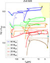 |
Fig. 1. Hertzsprung-Russel diagram for the new evolution models of this work (solid lines), compared with the models from Yusof et al. (2022, dashed lines). The empty, dark yellow, and dark cyan circles represent the end of the H-core, the beginning of the He-core, and the end of the He-core burning stages, respectively. The yellow shaded region corresponds to the zone beyond the Humphreys-Davidson limit, in which LBV stars are expected to be found (Humphreys et al. 2016). |
3.1. Evolution during the main-sequence stage
In line with Krtička & Kubát (2018) and Gormaz-Matamala et al. (2022b), we see that the mass-loss rates from K24 are ∼3 times (for Mzams = 20 M⊙) to ∼5 times (for Mzams = 60 M⊙) weaker than V01. For main-sequence stars, as also observed for low-metallicity environments (Gormaz-Matamala et al. 2024), a reduced mass loss also implies a reduced loss of angular momentum, resulting in a nearly constant rotational velocity during the first half of the main sequence prior to the final decrease in velocity. This differs from the abrupt initial deceleration predicted by older models shown in Fig. 2. Although we started our models with lower vrot, ini than Yusof et al. (2022), the average rotational velocity ⟨vrot⟩ for the most massive cases is therefore higher.
The combination of the lower initial Ṁ and lower initial vrot produces a less homogeneous inner structure. Reduced mass loss causes stars to retain more of their outer envelopes, whereas a lower rotation produces a less efficient internal mixing. Thus, the models show redder tracks throughout the main sequence, as shown in Fig. 1 (and thus, a larger radial expansion) as a consequence of the less homogeneous chemical evolution (Maeder 1987; Meynet et al. 2013). They therefore end the main sequence with cooler stellar temperatures. This scenario was also observed when only isolated changes in the Ṁ formula were implemented (Gormaz-Matamala et al. 2023), which demonstrates that the lower mass loss is far more effective than the reduced rotation. A less efficient mixing also means a shorter lifetime for the H-core burning process because the core is less likely to be refilled with hydrogen from the upper layers. It also means a more moderate chemical enrichment in the stellar surface, where the new models exhibit larger fractions of hydrogen than the models from Yusof et al. (2022). Similarly, the CNO abundances at the stellar surface are affected. The H-burning CNO bi-cycle causes nitrogen to accumulate in the core at the expense of carbon and oxygen. These changes are subsequently transferred to the surface through rotational mixing and the removal of outer envelopes, as outlined by Przybilla et al. (2010) and Maeder et al. (2014). Consequently, the new models (with reduced mass loss and mixing) exhibit smaller mass fractions of nitrogen at the end of the main sequence, while larger mass fractions of carbon and oxygen are observed. The less homogeneous structure is also expressed in lower fractions for the convective core mass (Fig. 3) because the total mass is higher.
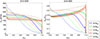 |
Fig. 2. Evolution of the rotational velocity expressed as absolute magnitude vrot (left panel) and of the angular velocity as a fraction of the critical velocity Ω/Ωcrit (right panel) as a function of the H-core burning lifetime τH. The solid and dashed lines represent new and old models, respectively, as in Fig. 1. |
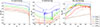 |
Fig. 3. Evolution of the convective cores as fractions of the total stellar mass for our models during the H-core, H-shell, and He-core stages. The solid and dashed lines represent new and old models, respectively, as in Fig. 1. |
The differences between the new evolution models and those from Yusof et al. (2022) are more prominent at higher initial mass. For Mzams = 32 M⊙ and above, the reduction of stellar mass at the end of the H-core burning is more moderate for the new models. With updated mass-loss rate prescriptions, our model with an initial mass of Mzams = 32 M⊙ loses only 1 M⊙ during the main sequence, compared to ≈5 M⊙ predicted by the old model. Similarly, our model with Mzams = 60 loses only ≈5 M⊙ during the main sequence, compared to ≈25 M⊙ predicted by the old model. Hence, while Yusof et al. (2022) predicted that stars lose up to half of their initial masses during the H-core burning, our new models predict a loss of only ∼8% at most5. These significant differences suggest substantial changes in subsequent evolutionary stages, even when other wind recipes remained unchanged. We discuss this further below.
3.2. Evolution in the post-main-sequence stage
3.2.1. H-shell burning stage
After the hydrogen depletion at the core, the H-shell burning stage begins. It contracts the (now) He core and expands the outer layers (Groh et al. 2014). For this reason, all of our models quickly expand radially when they cross the HR diagram horizontally at almost constant luminosity. This is the so-called Hertzsprung gap (HG, Hurley et al. 2000), which reaches temperatures below 10 kK at the end of the HG. The crossing of Teff = 10 kK implies a change in the mass-loss rate recipe from K24 to de Jager et al. (1988), but the rapid expansion just culminates when the He-core reaches temperatures that are high enough to start the He-burning process (He ignition), which occurs in the red region of the HR diagram, as shown in Fig. 1.
During this expansion, the stellar mass-loss rate peaks at Teff ∼ 15 kK according to the K24 formula (A.1), and thus, the removed mass is lower than predicted by previous models due to the bi-stability jump. This is explicitly shown in Fig. 4, where the overall mass loss is lower for new models, and the jumps predicted by V01 no longer exist. The differences in the mass-loss crossing of the HG can reach up to two orders of magnitude. The new values for Ṁ ∼ 10−7 − 10−6 M⊙ yr−1 agree better with the m-CAK δ-slow wind solutions for the regime of B supergiants (Araya et al. 2021; Venero et al. 2024). The radial expansion across the Hertzsprung gap is also faster because we chose the Ledoux criterion instead of Schwarzschild’s: the (molecular weight) μ-gradient at the border of the core prevents convection in the deep layers, which weakens the support of the star, which hence crosses the Hertzsprung gap rapidly (Sibony et al. 2023). In the case of the 20 M⊙, this occurs too quickly (relative to the Kelvin-Helmholtz timescale) for thermal equilibrium, and its radiation therefore expands the envelope, which explains the drop in luminosity. Table 3 shows the time required for the star to evolve from the end of the main sequence to the end of the HG: the lower mass loss combined with the shorter crossing time means that new models lose an amount of mass that is almost negligible when they cross the HG. Consequently, the envelope removal is almost negligible, so that we can assume that the chemical composition of the stars is almost the same as is tabulated for the end of the H-core burning.
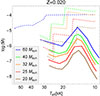 |
Fig. 4. Mass-loss rates after H depletion as a function of the effective temperature for the evolution tracks from Yusof et al. (2022, dashed lines) and the tracks from this work (solid lines). The solid and dashed lines represent new and old models, respectively, as in Fig. 1. |
Time interval and mass lost during the crossing of the Hertzsprung gap according to our models.
3.2.2. He-core and C-core burning stages
The higher Ṁ from Yang et al. (2023) means that our model of Mzams = 40 M⊙ experiences a strong mass removal of the order of log ṀY23 ≃ −1.8 when it crosses the threshold of Teff = 5 kK, with a subsequent drift back to Teff > 5 kK. It therefore enters a loop between the two wind regimes of dJ88 and Y23. This is a numerical artefact, but it can be physically interpreted as our 40 M⊙ being subject to strong and variable outflows of ∼5 kK, which prevents the star from becoming a RSG. The higher Ṁ from Yang et al. (2023) for Teff < 5 kK therefore helps us to preserve the upper Humphreys-Davidson limit (Humphreys et al. 2016) on log(L/L⊙)≃5.5 from Davies et al. (2018) and McDonald et al. (2022), and it also reduces the total time spent in the RSG phase (Zapartas et al. 2025). The higher ṀY23 removes more mass during the entire evolution of our stars (as shown by the black lines in Fig. 5). Additionally, the more efficient peeling-off effect during the RSG phase reduces the minimum initial mass required for a star to become a Wolf-Rayet star. RSGs evolve blueward in the HR diagram when the mass of their convective cores reaches 60% of the total mass (Meynet et al. 2015). Even though new models start their He ignition with lower Mcore/M* ratios (left panel of Fig. 3), the additional removal of the outer envelopes compensates for this condition, and thus, all stars with Mzams ≥ 25 M⊙ continue to evolve into WR stars. The exception is our 20 M⊙ model, which reaches the RSG phase with a luminosity log(L/L⊙) < 5.0 (in contrast with the ≃5.2 from Yusof et al. 2022). This results in a lower ṀRSG and in a poorer chemical enrichment at the stellar surface at the end of the He-core and C-core burning stages.
 |
Fig. 5. Evolution of the surface abundances for hydrogen, helium, carbon, nitrogen, and oxygen for the models that reach the WR phase. The black lines represent the total mass fraction, M*/Mzams. The nitrogen abundance is multiplied by 10 for illustrative purposes. |
The remaining models continue to evolve towards the Wolf-Rayet phases. For stars with 25 and 32 solar masses, the new models predict lower final masses at the end of their lives (8.68 and 8.41 M⊙, respectively), which are even lower than the final mass predicted for Mzams = 20 M⊙. After the RSG phase, which corresponds to the abrupt drops in mass fraction and hydrogen, the new models with 25 and 32 M⊙ have lower masses (than the old models), whereas the opposite occurs for models with 40 and 60 M⊙. All models leave the RSG phase with a higher H/He ratio, however, as a consequence of the lower mixing during the earlier evolutionary stages. According to the recipes of Nugis & Lamers (2000) and Gräfener & Hamann (2008), ṀWR is more moderate for stars with higher H/He, and thus, WR stars will initially lose less mass and envelope. This initially lower ṀWR creates a stronger inhomogeneity in the inner stellar structure, however, which causes the evolution tracks to move more redwards during their WR lifetime, as noted in the HR diagram. They therefore experience inflation episodes due to supra-Eddington layers (Ekström et al. 2012). As a result, the envelope removal of these WR stars is sped up as they continue to evolve. The case of Mzams = 25 M⊙ is particularly noteworthy because it causes the new track to continue evolve towards the WC phase (in which carbon and oxygen make up ∼70% of the surface composition), in contrast with the old model, which predicts a final state as an almost pure He star (≃96% of its surface composition).
For the most massive cases, this effect is less relevant. The model with 32 M⊙ has a lower mass, but with a chemical composition at the end of the C-core burning stage comparable to the composition predicted by Yusof et al. (2022). For 40 M⊙, ṀY23 prevented the model from becoming an RSG star, but still resulted in a significant mass removal that compensated for initial deviations during the OB-type mass-loss phase. This explains why the final mass and final chemical compositions are quite similar for the old and new models. For 60 M⊙, the deviations during the main sequence were substantial enough to persist through subsequent stages, particularly since it never became an RSG. This resulted in a final mass predicted by the new model (21.3 M⊙) that is higher by approximately 65% than that of the old model.
4. Stellar properties in the Galactic centre
We evaluate the current evolutionary status of the massive stars in the Galactic centre according to our new evolution tracks. We are particularly interested in the chemical surface abundance of these stars because this affects the accretion onto the central supermassive black hole (e.g., Calderón et al. 2025). Despite the known kinematics of hundreds of massive stars in the central parsec of the Milky Way (von Fellenberg et al. 2022), the only stars with measured stellar properties are the sample of WR stars from Martins et al. (2007) and the so-called S-stars from Habibi et al. (2017). These S-stars, however, are spectroscopically B dwarfs (i.e. early main-sequence stars without any wind) with initial masses between ∼7 − 15 M⊙, whose evolutionary status is barely affected by the updated wind mass-loss rate prescriptions. Therefore, our observational analysis focused on the sample of WR stars.
4.1. Theoretical predictions for observed WR stars
For WR stars in the Galactic centre, the known sample includes the spectral types Ofpe/WN9, WN (subtypes 5 to 8), WN/C, and WC (subtypes 8 and 9). Their determined temperatures, luminosities, and abundances are given by Martins et al. (2007, see their Table 2).
4.1.1. Ofpe/WN9 and WN stars
The left panel of Fig. 6 shows the hydrogen fraction as a function of luminosity, starting from the He-ignition, for the old and new evolution tracks. This figure is analogous to Fig. 21 by Martins et al. (2007), where the tracks were from Meynet & Maeder (2005). Based on this, it was deduced that Ofpe/WN9 are immediate precursors of WR stars. Because the post-MS stellar evolution for stars in the range of 25 to 60 M⊙ is at almost constant luminosity, however, the plane Xsurf − L* is not enough to provide insights into the evolutionary status of these stars. We therefore added a second panel on the right that shows the hydrogen mass fraction, but as a function of the stellar temperature (the radius rescaling is taken from Meynet & Maeder 2005), also from the start of the He-core burning. All our models started He ignition with Teff < 10 kK (Fig. 1). They therefore began as YSG/RSG stars that lost surface hydrogen at an almost constant temperature before they continued to evolving bluewards post-YSG/RSG. New models predict the post-YSG/RSG evolution to be richer in H than their counterparts predicted by Yusof et al. (2022), which also makes them redder. Hence, the hydrogen mass fractions predicted by our evolution models for post-RSG and post-YSG phases match the high XH exhibited by these Ofpe/WN9 stars well, even though some of these Ofpe/WN9 are in a quiescent LBV state (Crowther et al. 1995a), in particular, the stars with the highest hydrogen content.
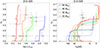 |
Fig. 6. Left panel: Hydrogen mass fraction at the stellar surface as a function of the stellar luminosity from the H-core ignition to the C-core depletion. Right panel: Hydrogen mass fraction at the stellar surface as a function of the stellar temperature from He ignition to the C-core depletion. The grey stars and triangles represent the observational values calculated by Martins et al. (2007) for Ofpe/WN9 and WN stars, respectively. The solid and dashed lines represent new and old models, respectively, as in Fig. 1. |
All the evidence supports the hypothesis that Ofpe/WN9 are precursors of late-type WN stars, but this does not necessarily mean that WN8 is the immediate stage after. Figure 6 also shows that with the exception of the 60 M⊙ model, the new tracks for post Ofpe/WN9 phase start to decrease their temperatures as the surface hydrogen decreases below ∼20%. Considering XH = 0.2 to be the threshold between Ofpe/WN9 and WNL stars (a reasonable assumption, given the observed abundances of the Martins et al. 2007, sample), we suggest that the temporal sequence for the initial mass range ∼25 − 40 M⊙ does not decrease from WN8 to earlier WNL (subtypes 7 and 6), but increases (Ofpe/WN9→WN6→WN7→WN8→...) or is even non-monotonic. This statement is not conclusive because the actual distinctions between the WN subtypes are not based on evolutionary properties, but on the properties of the He and N lines (Smith et al. 1996; Crowther 2007). The surface nitrogen abundance increases from the beginning of the WR phase (Fig. 5), however, whereas the observed WN8 and WN8/WC9 stars contain more nitrogen than their earlier siblings WN 5/6 and WN 7 (Martins et al. 2007, Table 2). This supports our assessment. This means that WN8 stars in the GC are closer to the other subtypes WN5-7 than to Ofpe/WN9, and they should therefore be included in the same WNL subcategory for a posteriori wind colliding models (compare with the input of sub-groups of WR stars adopted by Calderón et al. 2025).
4.1.2. WN/C and WC stars
WN/C stars are WR stars in which the surface nitrogen and carbon are in equilibrium (C/N ratio of the order of 1). This spectral type is expected to be found for stars born with masses between ∼30 and 60 M⊙, which are massive enough to show He-burning nuclear waste (carbon) before their core collapse, but not so massive as not to be quickly depleted of all their surface hydrogen before they become WC (Meynet & Maeder 2003). When the WR phase starts, the stellar surface is very poor in C because the CNO cycle converts carbon into nitrogen, but it becomes C rich as the products of He burning (carbon and oxygen) start to appear in the outer envelopes. The nitrogen abundance also increases during the WR phase, as shown in Fig. 5, but at a lower rate than carbon. The ratio C/N therefore increases.
These evolutionary diagnostics are based on solar metallicity (assuming Z⊙ = 0.02), but still fits our set of new evolution models quite well. Figure 7 shows the evolution of the C/He ratio post-YSG/RSG as a function of the stellar luminosity (left panel) and temperature (right panel) for the new and old tracks. The surface carbon abundance increases as the WR star temperature decreases slightly, and the WN/C stars from Martins et al. (2007) are located before the end of this redwards drift. As for the Martins WC stars, the C/He ratio coincides with the rapid jump in temperature in the new models, which is overcome with the removal of the last traces of hydrogen (i.e. at the end of any WN signature). Still, this behaviour of C/He versus Teff is found for both old and new evolution tracks. The differences arise when we analyse the C/He ratio against the luminosity. Our 25 M⊙ model continued to evolve towards the WC phase and therefore matches the dimmer WN/C and WC stars analysed by Martins et al. (2007) better, without the need of invoking binary evolution.
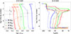 |
Fig. 7. Left panel: Carbon-to-helium ratio (by number) at the stellar surface as a function of the stellar luminosity from the post-YSG/RSG phase to C depletion. Right panel: Carbon-to-helium ratio (by number) at the stellar surface as a function of the stellar temperature from the post-YSG/RSG phase to C depletion. The grey diamonds and circles represent the observational values calculated by Martins et al. (2007) for WN/C and WC stars, respectively. The solid and dashed lines represent new and old models, respectively, as in Fig. 1. |
When the latest traces of hydrogen are still present in the outer envelope of our structure models, the calculated opacity for this outer envelope becomes uncertain, and subsequently, the radius can be numerically inflated, with the respective drop in the temperature. This opacity effect is an inherent condition produced by the mismatch between (hydrostatic) evolution models and (expanding) atmospheric models. Even though deep expanding atmospheric models can correct the expected temperatures predicted in GENEC models subject to envelope inflation, this requires considerable computational effort and has only been implemented for the main-sequence stage of very massive stars (Josiek et al. 2025). This opacity effect represents a very small fraction of the WR lifetime, however, and does not interfere with the chemical composition or temperatures measured for the WN/C and WC stars in the sample. Therefore, despite this issue and the associated error bars in the infrared spectra, the new evolution tracks at super solar metallicity can adequately reproduce the observational diagnostics for the massive stars of the Galactic centre.
4.2. Evolutionary phases
Following Martinet et al. (2023), we proceeded to define the WR subtypes as evolutionary stages. We cannot use spectroscopic criteria for these categories (because we did not provide synthetic spectra) and therefore used some abundances and the temperature calculated by our models as criteria:
-
Ofpe/WN9: WR star with XH ≥ 0.2 and T* ≤ 30 kK.
-
eWNL: WR star with XH ≥ 10−5.
-
eWNE: WR star and XH < 10−5 and XN > XC.
-
WN/C: WR star with −0.5 < log(XC/XN) < 0.5.
-
WC: WR star with log T* < 5.20 and (XC + XO)/XHe < 1.6.
The threshold for Ofpe/WN9 stars comes from the analysis of Sect. 4.1.1 and from the parameters calculated by Crowther et al. (1995a). The boundary XH = 10−5 for eWNL and eWNE (where the ‘e’ stands for ‘evolutionary’, following Foellmi et al. 2003) comes from Georgy et al. (2012). The boundaries for the WN/C phase agree with the C/N values reported by Crowther et al. (1995b). The separation between WC and WO comes from the C, O, and He abundances measured by Aadland et al. (2022).
We highlight the segment of each of the Wolf-Rayet phases (Ofpe/WN9, WNL, WN/C, and WC) in the HR diagram in Fig. 8, together with the GC stars from Martins et al. (2007). In general, we note that the observed and evolutionary spectral type agree, with some minor discrepancies due to the lack of unified criteria. For example, our C/N abundances for the WN/C phase differ from the boundaries used by Georgy et al. (2012), where WN/C stars are additionally expected to be H poor. In our case, we still find traces of hydrogen at the surface of WN/C stars because the chemical evolution consequence of lower winds is moderate. This is shown in Fig. 9, where the new evolution models predict that the stars become richer in carbon before the total depletion of hydrogen from the stellar surface. In contrast, old models predicted stars with Xsurf ≤ 10−5 and XN > XC, which is in the category of eWNE stars. Thus, all our evolution models predict that (H-rich) WNL stars evolve into WN/C without passing through eWNE phase. This is consistent with the lack of early-type WN stars in the sample of Martins et al. (2007), where the earliest WN star was 16SE2 with a spectroscopic subtype WN5/6. As mentioned in Sect. 4.1.1, the low nitrogen content of 16SE2 also suggests that this WN5/6 might be located before the WN7-8 stars in the evolutionary sequence, which strengthens the idea that the WNL phase is the direct precursor of WN/C for the mass and metallicity range we analysed. Again, the aforementioned bypass to the eWNE phase is only based on the abundance criteria from the evolution models and not from spectroscopic features, and it therefore cannot be taken as a full absence of WNE stars in the GC.
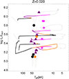 |
Fig. 8. Hertzsprung-Russel diagram showing the position of the spectroscopic phases Ofpe/WN9 (magenta), WN (purple), WN/C (orange), and WC (black). The observed stars from Martins et al. (2007) are shown with the same symbols as in Figs. 6 and 7. |
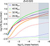 |
Fig. 9. Evolution of the C/N ratio in the evolution models as the stars loose their last 1% of hydrogen in the outer layer. The blue shaded region represents XH ≤ 10−5 and XC ≥ XN, and the grey shaded region shows XH ≥ 10−5 and XC ≤ XN. The solid and dashed lines represent the new and old models, respectively, as in Fig. 1. |
We calculated the surface abundances for hydrogen, helium, carbon, nitrogen, and oxygen for our evolution models during the Ofpe/WN9, WNL, WN/C, and WC phases. The individual surface abundances still change within the same spectral subtypes, and we therefore calculated the time-averaged abundances, defined as
 (1)
(1)
where Δτphase = tf − ti (tf is the final time, and ti is the initial time) is the lifetime of the respective subtype, and the corresponding uncertainties as the standard deviations,
![Mathematical equation: $$ \begin{aligned} \sigma (X_{\rm elem}) = \sqrt{\frac{1}{\Delta \tau _{\rm phase}}\int _{t_{\rm i}}^{t_{\rm f}}[X_{\rm elem}(t)-\langle X_{\rm elem}\rangle ]^2\,\mathrm{d}t}. \end{aligned} $$](/articles/aa/full_html/2026/02/aa56877-25/aa56877-25-eq2.gif) (2)
(2)
The results for the WR phases are shown in Table 4, together with the lifetimes of the spectroscopic phases and the average mass-loss rate (calculated as ΔM*, lost/Δτphase). WR stars are less chemically evolved at their surface for lower initial masses. For Ofpe/WN9 phase, the model with Mzams = 25 M⊙ presents the largest hydrogen mass fraction because less mass was removed than from their counterparts, which is also shown in the right panel of Fig. 6. It also has the longest lifetime because the mass loss during this Ofpe/WN9 is most reduced. For the WN phase, the abundances have a larger standard deviation as a consequence of the quick changes in the chemical composition. For WN/C and WC stars, the abundances are mostly of the same orders of magnitude, with the notable exception of Mzams = 25 M⊙. This model alone reaches the end of the He-core burning stage in the WN/C phase and then becomes a WC star only at the very end before the end of C-core burning.
Time-averaged surface abundances in the different WR spectroscopic phases of our evolution models.
These tabulated abundances represent an important upgrade for the modelling of the Galactic centre environment around Sgr A*. Recent works have adopted the chemical composition from a selection of observed WR stars, first compiled by Russell et al. (2017) and used in that study and by Wang et al. (2020), Balakrishnan et al. (2024), to produce synthetic X-ray spectra from hydrodynamical simulations, and more recently, by Calderón et al. (2025) and Labaj et al. (2025) as a simulation ingredient. These stars were classified as WC8-9, WN5-7, WN8-9, and Ofpe/WN9 stars, with the last two subtypes treated as a single category, with XH = 11.5 and XHe = 82.5. Our evolution models suggest, however, that WN8 might not be the direct descendant of Ofpe/WN9, and we therefore consider that they should not be combined. Ofpe/WN9 stars are expected to have higher hydrogen abundances, which agrees with the spectral diagnostics performed by Martins et al. (2007). Likewise, evolutionary WN5-8 stars as a whole category are now expected to contain a higher fraction of hydrogen due to their previous evolutionary stages, although with large standard deviations. On the other hand, the average abundances for WC agree better with the data tabulated by Russell et al. (2017), with the exception of our 25 M⊙ model, for the reasons given in the previous paragraph.
Our new abundances lie in general in between those used previously in the literature for hydrodynamical simulations of the Galactic centre WR winds, namely either solar with a three times enhanced metallicity (e.g., Calderón et al. 2020a), or the Russell et al. (2017) tabulated abundances (Calderón et al. 2025). The former resulted in a higher rate of radiative cooling after the wind shock collisions, and the subsequent formation of clumps and even a cold disc that increased the accretion on to Sgr A*, while in the latter, these effects were suppressed. Updated hydrodynamical models should be developed using the abundances obtained in this work, for which not only the spectral type of the stars can be used, but also estimates of their masses when available.
5. Summary and conclusions
We showed a set of evolutionary tracks using the Geneva evolution code (GENEC) for stars with initial masses from 20 to 60 M⊙, with new mass-loss rate recipes for the winds of OB-type stars (Krtička et al. 2024) and RSGs (Yang et al. 2023). Because of the lower Ṁ during the main-sequence stage and the Hertzsprung gap, the stars retain more than ≈92% of their initial masses prior to the stronger dust-driven mass loss in the red part of the HRD, where the star finally looses most of its envelopes.
These changes in the mass-loss history create Wolf-Rayet stars with a less evolved chemical evolution (and subsequently, that are cooler) in comparison with previous models (Yusof et al. 2022). After the Ofpe/WN9 spectral phase, the stars stay as late-type WN and become WN/C, bypassing the early-type WN spectral phase. This scenario agrees with the observed population of WR in the GC (Martins et al. 2007), where the late type clearly dominates for all WN, WN/C, and WC subtypes. Based on this scenario, we tabulated the respective mean surface abundances and lifetimes of each of the WR spectroscopic phases to provide a more robust framework for the study of the colliding winds from the population of WR stars around the supermassive black hole Sgr A* at the centre of the Milky Way (Calderón et al. 2025).
The results we presented are the most recent in terms of stellar wind theory, stellar evolution at high metallicity environments, and observations of the Galactic centre. Because Z = 0.020 represents a lower threshold for the probable metallicity of the centre of the Milky Way, further studies need to be performed with a wind theory than can provide adequate values of the mass loss at higher Z. Likewise, new spectroscopic measurements are needed for the population of WR stars in the GC in order to decrease the uncertainties in the currently known abundances, as well as the uncertainties in their actual wind properties (Ṁ and v∞). Nevertheless, the new evolutionary tracks we introduced and the surface abundances predicted for WR stages represent an important upgrade in our understanding of the physical conditions in the Galactic centre, and they will be the initial starting point for future population synthesis studies for colliding winds.
Acknowledgments
We acknowledge useful discussions with Diego Calderón, Chris Russell, Wasif Shaqil, and Sebastiano von Fellenberg. ACGM thanks the support from project 10108195 MERIT (MSCA-COFUND Horizon Europe). ACGM and JC acknowledge the support from the Max Planck Society through a “Partner Group” grant. JC acknowledges financial support from ANID – FONDECYT Regular 1251444, and Millennium Science Initiative Program NCN2023_002. BK and JK acknowledge support from the Grant Agency of the Czech Republic (GAČR 25-15910S). SE acknowledges support from the Swiss National Science Foundation (SNSF), grant number 212143. The Astronomical Institute of the Czech Academy of Sciences in Ondřejov is supported by the project RVO: 67985815. Computational resources were provided by the e-INFRA CZ project (ID:90254), supported by the Ministry of Education, Youth and Sports of the Czech Republic.
References
- Aadland, E., Massey, P., Hillier, D. J., et al. 2022, ApJ, 931, 157 [NASA ADS] [CrossRef] [Google Scholar]
- Antoniadis, K., Bonanos, A. Z., de Wit, S., et al. 2024, A&A, 686, A88 [NASA ADS] [CrossRef] [EDP Sciences] [Google Scholar]
- Antoniadis, K., Zapartas, E., Bonanos, A. Z., et al. 2025, A&A, 702, A178 [NASA ADS] [CrossRef] [EDP Sciences] [Google Scholar]
- Araya, I., Christen, A., Curé, M., et al. 2021, MNRAS, 504, 2550 [NASA ADS] [CrossRef] [Google Scholar]
- Asplund, M., Grevesse, N., Sauval, A. J., & Scott, P. 2009, ARA&A, 47, 481 [NASA ADS] [CrossRef] [Google Scholar]
- Balakrishnan, M., Russell, C. M. P., Corrales, L., et al. 2024, ApJ, 974, 99 [NASA ADS] [CrossRef] [Google Scholar]
- Bartko, H., Martins, F., Fritz, T. K., et al. 2009, ApJ, 697, 1741 [Google Scholar]
- Bartko, H., Martins, F., Trippe, S., et al. 2010, ApJ, 708, 834 [Google Scholar]
- Beasor, E. R., Davies, B., Smith, N., et al. 2023, MNRAS, 524, 2460 [Google Scholar]
- Bestenlehner, J. M. 2020, MNRAS, 493, 3938 [Google Scholar]
- Björklund, R., Sundqvist, J. O., Puls, J., & Najarro, F. 2021, A&A, 648, A36 [EDP Sciences] [Google Scholar]
- Björklund, R., Sundqvist, J. O., Singh, S. M., Puls, J., & Najarro, F. 2023, A&A, 676, A109 [NASA ADS] [CrossRef] [EDP Sciences] [Google Scholar]
- Calderón, D., Ballone, A., Cuadra, J., et al. 2016, MNRAS, 455, 4388 [Google Scholar]
- Calderón, D., Cuadra, J., Schartmann, M., Burkert, A., & Russell, C. M. P. 2020a, ApJ, 888, L2 [Google Scholar]
- Calderón, D., Cuadra, J., Schartmann, M., et al. 2020b, MNRAS, 493, 447 [Google Scholar]
- Calderón, D., Cuadra, J., Russell, C. M. P., et al. 2025, A&A, 693, A180 [NASA ADS] [CrossRef] [EDP Sciences] [Google Scholar]
- Choi, J., Dotter, A., Conroy, C., et al. 2016, ApJ, 823, 102 [Google Scholar]
- Ciurlo, A., Morris, M. R., Campbell, R. D., et al. 2021, ApJ, 910, 143 [NASA ADS] [CrossRef] [Google Scholar]
- Costa, G., Shepherd, K. G., Bressan, A., et al. 2025, A&A, 694, A193 [NASA ADS] [CrossRef] [EDP Sciences] [Google Scholar]
- Crowther, P. A. 2007, ARA&A, 45, 177 [Google Scholar]
- Crowther, P. A., Hillier, D. J., & Smith, L. J. 1995a, A&A, 293, 172 [NASA ADS] [Google Scholar]
- Crowther, P. A., Smith, L. J., & Willis, A. J. 1995b, A&A, 304, 269 [NASA ADS] [Google Scholar]
- Cuadra, J., Nayakshin, S., Springel, V., & Di Matteo, T. 2005, MNRAS, 360, L55 [CrossRef] [Google Scholar]
- Cuadra, J., Nayakshin, S., & Martins, F. 2008, MNRAS, 383, 458 [NASA ADS] [Google Scholar]
- Cuadra, J., Nayakshin, S., & Wang, Q. D. 2015, MNRAS, 450, 277 [CrossRef] [Google Scholar]
- Curé, M. 2004, ApJ, 614, 929 [CrossRef] [Google Scholar]
- Curé, M., & Rial, D. F. 2007, Astron. Nachr., 328, 513 [CrossRef] [Google Scholar]
- Davies, B., Crowther, P. A., & Beasor, E. R. 2018, MNRAS, 478, 3138 [NASA ADS] [CrossRef] [Google Scholar]
- de Burgos, A., Keszthelyi, Z., Simón-Díaz, S., & Urbaneja, M. A. 2024, A&A, 687, L16 [NASA ADS] [CrossRef] [EDP Sciences] [Google Scholar]
- de Jager, C., Nieuwenhuijzen, H., & van der Hucht, K. A. 1988, A&AS, 72, 259 [NASA ADS] [Google Scholar]
- Decin, L., Richards, A. M. S., Marchant, P., & Sana, H. 2024, A&A, 681, A17 [NASA ADS] [CrossRef] [EDP Sciences] [Google Scholar]
- Eggenberger, P., Meynet, G., Maeder, A., et al. 2008, Ap&SS, 316, 43 [Google Scholar]
- Ekström, S., Georgy, C., Eggenberger, P., et al. 2012, A&A, 537, A146 [Google Scholar]
- Foellmi, C., Moffat, A. F. J., & Guerrero, M. A. 2003, MNRAS, 338, 1025 [NASA ADS] [CrossRef] [Google Scholar]
- Genzel, R., Eisenhauer, F., & Gillessen, S. 2010, Rev. Mod. Phys., 82, 3121 [Google Scholar]
- Georgy, C., Meynet, G., & Maeder, A. 2011, A&A, 527, A52 [NASA ADS] [CrossRef] [EDP Sciences] [Google Scholar]
- Georgy, C., Ekström, S., Meynet, G., et al. 2012, A&A, 542, A29 [NASA ADS] [CrossRef] [EDP Sciences] [Google Scholar]
- Georgy, C., Saio, H., & Meynet, G. 2014, MNRAS, 439, L6 [Google Scholar]
- Ghez, A. M., Duchêne, G., Matthews, K., et al. 2003, ApJ, 586, L127 [Google Scholar]
- Gillessen, S., Genzel, R., Fritz, T. K., et al. 2012, Nature, 481, 51 [Google Scholar]
- Gillessen, S., Eisenhauer, F., Cuadra, J., et al. 2026, A&A, in press, https://doi.org/10.1051/0004-6361/202555808 [Google Scholar]
- Goldman, S. R., van Loon, J. T., Zijlstra, A. A., et al. 2017, MNRAS, 465, 403 [Google Scholar]
- Gómez-González, V. M. A., Oskinova, L. M., Hamann, W. R., et al. 2025, A&A, 695, A197 [NASA ADS] [CrossRef] [EDP Sciences] [Google Scholar]
- Gormaz-Matamala, A. C., Curé, M., Cidale, L. S., & Venero, R. O. J. 2019, ApJ, 873, 131 [NASA ADS] [CrossRef] [Google Scholar]
- Gormaz-Matamala, A. C., Curé, M., Meynet, G., et al. 2022a, A&A, 665, A133 [NASA ADS] [CrossRef] [EDP Sciences] [Google Scholar]
- Gormaz-Matamala, A. C., Curé, M., Lobel, A., et al. 2022b, A&A, 661, A51 [NASA ADS] [CrossRef] [EDP Sciences] [Google Scholar]
- Gormaz-Matamala, A. C., Cuadra, J., Meynet, G., & Curé, M. 2023, A&A, 673, A109 [NASA ADS] [CrossRef] [EDP Sciences] [Google Scholar]
- Gormaz-Matamala, A. C., Cuadra, J., Ekström, S., et al. 2024, A&A, 687, A290 [NASA ADS] [CrossRef] [EDP Sciences] [Google Scholar]
- Gormaz-Matamala, A. C., Romagnolo, A., & Belczynski, K. 2025, A&A, 696, A72 [NASA ADS] [CrossRef] [EDP Sciences] [Google Scholar]
- Gräfener, G., & Hamann, W. R. 2008, A&A, 482, 945 [Google Scholar]
- Groh, J. H., Meynet, G., Ekström, S., & Georgy, C. 2014, A&A, 564, A30 [NASA ADS] [CrossRef] [EDP Sciences] [Google Scholar]
- Habibi, M., Gillessen, S., Martins, F., et al. 2017, ApJ, 847, 120 [Google Scholar]
- Hayden, M. R., Holtzman, J. A., Bovy, J., et al. 2014, AJ, 147, 116 [NASA ADS] [CrossRef] [Google Scholar]
- Humphreys, R. M., & Jones, T. J. 2022, AJ, 163, 103 [NASA ADS] [CrossRef] [Google Scholar]
- Humphreys, R. M., Weis, K., Davidson, K., & Gordon, M. S. 2016, ApJ, 825, 64 [NASA ADS] [CrossRef] [Google Scholar]
- Hurley, J. R., Pols, O. R., & Tout, C. A. 2000, MNRAS, 315, 543 [Google Scholar]
- Josiek, J., Ekström, S., & Sander, A. A. C. 2024, A&A, 688, A71 [NASA ADS] [CrossRef] [EDP Sciences] [Google Scholar]
- Josiek, J., Sander, A. A. C., Bernini-Peron, M., et al. 2025, A&A, 697, A193 [NASA ADS] [CrossRef] [EDP Sciences] [Google Scholar]
- Kee, N. D., Sundqvist, J. O., Decin, L., de Koter, A., & Sana, H. 2021, A&A, 646, A180 [NASA ADS] [CrossRef] [EDP Sciences] [Google Scholar]
- Krtička, J., & Kubát, J. 2017, A&A, 606, A31 [NASA ADS] [CrossRef] [EDP Sciences] [Google Scholar]
- Krtička, J., & Kubát, J. 2018, A&A, 612, A20 [NASA ADS] [CrossRef] [EDP Sciences] [Google Scholar]
- Krtička, J., Kubát, J., & Krtičková, I. 2021, A&A, 647, A28 [NASA ADS] [CrossRef] [EDP Sciences] [Google Scholar]
- Krtička, J., Kubát, J., & Krtičková, I. 2024, A&A, 681, A29 [NASA ADS] [CrossRef] [EDP Sciences] [Google Scholar]
- Kruckow, M. U., Andrews, J. J., Fragos, T., et al. 2024, A&A, 692, A141 [NASA ADS] [CrossRef] [EDP Sciences] [Google Scholar]
- Labaj, M., Ressler, S. M., Zajaček, M., et al. 2025, A&A, 702, A233 [NASA ADS] [CrossRef] [EDP Sciences] [Google Scholar]
- Liu, B., Sibony, Y., Meynet, G., & Bromm, V. 2025, ApJ, 980, L30 [Google Scholar]
- Lu, J. R., Do, T., Ghez, A. M., et al. 2013, ApJ, 764, 155 [NASA ADS] [CrossRef] [Google Scholar]
- Maeder, A. 1987, A&A, 178, 159 [NASA ADS] [Google Scholar]
- Maeder, A. 1997, A&A, 321, 134 [NASA ADS] [Google Scholar]
- Maeder, A., & Meynet, G. 2000, A&A, 361, 159 [NASA ADS] [Google Scholar]
- Maeder, A., Przybilla, N., Nieva, M.-F., et al. 2014, A&A, 565, A39 [NASA ADS] [CrossRef] [EDP Sciences] [Google Scholar]
- Mapelli, M., & Gualandris, A. 2016, Lect. Notes Phys., 905, 205 [NASA ADS] [CrossRef] [Google Scholar]
- Martinet, S., Meynet, G., Ekström, S., Georgy, C., & Hirschi, R. 2023, A&A, 679, A137 [NASA ADS] [CrossRef] [EDP Sciences] [Google Scholar]
- Martins, F., Genzel, R., Hillier, D. J., et al. 2007, A&A, 468, 233 [NASA ADS] [CrossRef] [EDP Sciences] [Google Scholar]
- McDonald, S. L. E., Davies, B., & Beasor, E. R. 2022, MNRAS, 510, 3132 [NASA ADS] [CrossRef] [Google Scholar]
- Meynet, G., & Maeder, A. 2003, A&A, 404, 975 [NASA ADS] [CrossRef] [EDP Sciences] [Google Scholar]
- Meynet, G., & Maeder, A. 2005, A&A, 429, 581 [CrossRef] [EDP Sciences] [Google Scholar]
- Meynet, G., Ekstrom, S., Maeder, A., et al. 2013, Lect. Notes Phys., 865, 3 [Google Scholar]
- Meynet, G., Chomienne, V., Ekström, S., et al. 2015, A&A, 575, A60 [NASA ADS] [CrossRef] [EDP Sciences] [Google Scholar]
- Murchikova, E. M., Phinney, E. S., Pancoast, A., & Blandford, R. D. 2019, Nature, 570, 83 [NASA ADS] [CrossRef] [Google Scholar]
- Nandal, D., Meynet, G., Ekström, S., et al. 2024, A&A, 684, A169 [NASA ADS] [CrossRef] [EDP Sciences] [Google Scholar]
- Nayakshin, S., Dehnen, W., Cuadra, J., & Genzel, R. 2006, MNRAS, 366, 1410 [Google Scholar]
- Nugis, T., & Lamers, H. J. G. L. M. 2000, A&A, 360, 227 [NASA ADS] [Google Scholar]
- Pauldrach, A. W. A., & Puls, J. 1990, A&A, 237, 409 [NASA ADS] [Google Scholar]
- Paumard, T., Genzel, R., Martins, F., et al. 2006, ApJ, 643, 1011 [NASA ADS] [CrossRef] [Google Scholar]
- Paxton, B., Bildsten, L., Dotter, A., et al. 2011, ApJS, 192, 3 [Google Scholar]
- Przybilla, N., Firnstein, M., Nieva, M. F., Meynet, G., & Maeder, A. 2010, A&A, 517, A38 [NASA ADS] [CrossRef] [EDP Sciences] [Google Scholar]
- Quataert, E. 2004, ApJ, 613, 322 [NASA ADS] [CrossRef] [Google Scholar]
- Ressler, S. M., Quataert, E., & Stone, J. M. 2018, MNRAS, 478, 3544 [NASA ADS] [CrossRef] [Google Scholar]
- Ressler, S. M., Quataert, E., & Stone, J. M. 2020, MNRAS, 492, 3272 [NASA ADS] [CrossRef] [Google Scholar]
- Romagnolo, A., Gormaz-Matamala, A. C., & Belczynski, K. 2024, ApJ, 964, L23 [NASA ADS] [CrossRef] [Google Scholar]
- Russell, C. M. P., Wang, Q. D., & Cuadra, J. 2017, MNRAS, 464, 4958 [CrossRef] [Google Scholar]
- Sander, A. A. C., & Vink, J. S. 2020, MNRAS, 499, 873 [Google Scholar]
- Sander, A. A. C., Lefever, R. R., Poniatowski, L. G., et al. 2023, A&A, 670, A83 [NASA ADS] [CrossRef] [EDP Sciences] [Google Scholar]
- Schödel, R., Ott, T., Genzel, R., et al. 2002, Nature, 419, 694 [Google Scholar]
- Sibony, Y., Georgy, C., Ekström, S., & Meynet, G. 2023, A&A, 680, A101 [NASA ADS] [CrossRef] [EDP Sciences] [Google Scholar]
- Smith, L. F., Shara, M. M., & Moffat, A. F. J. 1996, MNRAS, 281, 163 [NASA ADS] [CrossRef] [Google Scholar]
- Szécsi, D., Agrawal, P., Wünsch, R., & Langer, N. 2022, A&A, 658, A125 [NASA ADS] [CrossRef] [EDP Sciences] [Google Scholar]
- van Loon, J. T. 2025, Galaxies, 13, 72 [Google Scholar]
- Venero, R. O. J., Curé, M., Puls, J., et al. 2024, MNRAS, 527, 93 [Google Scholar]
- Verhamme, O., Sundqvist, J., de Koter, A., et al. 2024, A&A, 692, A91 [NASA ADS] [CrossRef] [EDP Sciences] [Google Scholar]
- Vink, J. S., de Koter, A., & Lamers, H. J. G. L. M. 1999, A&A, 350, 181 [Google Scholar]
- Vink, J. S., de Koter, A., & Lamers, H. J. G. L. M. 2001, A&A, 369, 574 [NASA ADS] [CrossRef] [EDP Sciences] [Google Scholar]
- von Fellenberg, S. D., Gillessen, S., Stadler, J., et al. 2022, ApJ, 932, L6 [NASA ADS] [CrossRef] [Google Scholar]
- Wang, Q. D., Li, J., Russell, C. M. P., & Cuadra, J. 2020, MNRAS, 492, 2481 [NASA ADS] [CrossRef] [Google Scholar]
- Yang, M., Bonanos, A. Z., Jiang, B., et al. 2023, A&A, 676, A84 [NASA ADS] [CrossRef] [EDP Sciences] [Google Scholar]
- Yusof, N., Hirschi, R., Eggenberger, P., et al. 2022, MNRAS, 511, 2814 [NASA ADS] [CrossRef] [Google Scholar]
- Zahn, J. P. 1992, A&A, 265, 115 [NASA ADS] [Google Scholar]
- Zapartas, E., de Wit, S., Antoniadis, K., et al. 2025, A&A, 697, A167 [NASA ADS] [CrossRef] [EDP Sciences] [Google Scholar]
Geneva-evolution-code.
Modules for Experiments in Stellar Astrophysics.
Bonn Optimised Stellar Tracks.
A higher mass-loss rate means a higher mass-loss rate at the same HRD location. The total RSG mass loss may change when the stellar track reaches the red region of the HRD at lower luminosities, as we show below.
This comparison was made considering the maximum mass Mzams = 60 M⊙ in our analysis. More massive cases would develop WR winds during the main sequence, either from extreme removal of their outer envelopes or due to the proximity to the Eddington limit (see Gormaz-Matamala et al. 2025). We therefore did not include them here.
Appendix A: Mass-loss rate recipes
For the winds of OB-type stars (Teff ≥ 10 kK) we use the formula from Krtička et al. (2024, Eq. 3 with coefficients from Table 3)
![Mathematical equation: $$ \begin{aligned} \log \dot{M}_{\rm K24}=&-13.82+0.358\log \left(\frac{Z}{Z_\odot }\right) +\log \left(\frac{L_*}{10^6L_\odot }\right)\times \left[1.52-0.11\log \left(\frac{Z}{Z_\odot }\right)\right]\nonumber \\&+13.82\log \Biggl \{\left[1.0+0.73\log \left(\frac{Z}{Z_\odot }\right)\right]\exp \left[-\frac{(T_{\rm eff}/\mathrm{kK}-14.16)^2}{3.58^2}\right]+3.84\exp \left[-\frac{(T_{\rm eff}/\mathrm{kK}-37.9)^2}{56.5^2}\right]\Biggr \}. \end{aligned} $$](/articles/aa/full_html/2026/02/aa56877-25/aa56877-25-eq3.gif) (A.1)
(A.1)
For the mass-loss rate of stars in the range of temperatures between 5 and 10 kK we use the linearised formula of de Jager et al. (1988)
 (A.2)
(A.2)
For the mass-loss rate of red supergiants (Teff ≤ 5 kK) we use the formula of Yang et al. (2023)
![Mathematical equation: $$ \begin{aligned} \log \dot{M}_{\rm Y23} = 0.45\left[\log \left(\frac{L_*}{L_\odot }\right)\right]^3 -5.26\left[\log \left(\frac{L_*}{L_\odot }\right)\right]^2 +20.93\log \left(\frac{L_*}{L_\odot }\right)-34.56. \end{aligned} $$](/articles/aa/full_html/2026/02/aa56877-25/aa56877-25-eq5.gif) (A.3)
(A.3)
For the wind of Wolf-Rayet stars with T* ≤ 70 kK we use Gräfener & Hamann (2008)
 (A.4)
(A.4)
with
![Mathematical equation: $$ \begin{aligned}&\beta (Z) = 1.727+0.25\log \left(\frac{Z}{Z_\odot }\right),\\&\Gamma _0(Z) = 0.325-0.301\log \left(\frac{Z}{Z_\odot }\right) -0.045\left[\log \left(\frac{Z}{Z_\odot }\right)\right]^2. \end{aligned} $$](/articles/aa/full_html/2026/02/aa56877-25/aa56877-25-eq7.gif)
Finally, for Wolf-Rayet stars out of the range covered by Gräfener & Hamann (2008), we use the formulae from Nugis & Lamers (2000) for WN and WC/WO phases
 (A.5)
(A.5)
 (A.6)
(A.6)
All Tables
Properties of the evolutionary tracks at the end of the He-core and the C-core burning stages.
Time interval and mass lost during the crossing of the Hertzsprung gap according to our models.
Time-averaged surface abundances in the different WR spectroscopic phases of our evolution models.
All Figures
|
Fig. 1. Hertzsprung-Russel diagram for the new evolution models of this work (solid lines), compared with the models from Yusof et al. (2022, dashed lines). The empty, dark yellow, and dark cyan circles represent the end of the H-core, the beginning of the He-core, and the end of the He-core burning stages, respectively. The yellow shaded region corresponds to the zone beyond the Humphreys-Davidson limit, in which LBV stars are expected to be found (Humphreys et al. 2016). |
| In the text | |
|
Fig. 2. Evolution of the rotational velocity expressed as absolute magnitude vrot (left panel) and of the angular velocity as a fraction of the critical velocity Ω/Ωcrit (right panel) as a function of the H-core burning lifetime τH. The solid and dashed lines represent new and old models, respectively, as in Fig. 1. |
| In the text | |
|
Fig. 3. Evolution of the convective cores as fractions of the total stellar mass for our models during the H-core, H-shell, and He-core stages. The solid and dashed lines represent new and old models, respectively, as in Fig. 1. |
| In the text | |
|
Fig. 4. Mass-loss rates after H depletion as a function of the effective temperature for the evolution tracks from Yusof et al. (2022, dashed lines) and the tracks from this work (solid lines). The solid and dashed lines represent new and old models, respectively, as in Fig. 1. |
| In the text | |
|
Fig. 5. Evolution of the surface abundances for hydrogen, helium, carbon, nitrogen, and oxygen for the models that reach the WR phase. The black lines represent the total mass fraction, M*/Mzams. The nitrogen abundance is multiplied by 10 for illustrative purposes. |
| In the text | |
|
Fig. 6. Left panel: Hydrogen mass fraction at the stellar surface as a function of the stellar luminosity from the H-core ignition to the C-core depletion. Right panel: Hydrogen mass fraction at the stellar surface as a function of the stellar temperature from He ignition to the C-core depletion. The grey stars and triangles represent the observational values calculated by Martins et al. (2007) for Ofpe/WN9 and WN stars, respectively. The solid and dashed lines represent new and old models, respectively, as in Fig. 1. |
| In the text | |
|
Fig. 7. Left panel: Carbon-to-helium ratio (by number) at the stellar surface as a function of the stellar luminosity from the post-YSG/RSG phase to C depletion. Right panel: Carbon-to-helium ratio (by number) at the stellar surface as a function of the stellar temperature from the post-YSG/RSG phase to C depletion. The grey diamonds and circles represent the observational values calculated by Martins et al. (2007) for WN/C and WC stars, respectively. The solid and dashed lines represent new and old models, respectively, as in Fig. 1. |
| In the text | |
|
Fig. 8. Hertzsprung-Russel diagram showing the position of the spectroscopic phases Ofpe/WN9 (magenta), WN (purple), WN/C (orange), and WC (black). The observed stars from Martins et al. (2007) are shown with the same symbols as in Figs. 6 and 7. |
| In the text | |
|
Fig. 9. Evolution of the C/N ratio in the evolution models as the stars loose their last 1% of hydrogen in the outer layer. The blue shaded region represents XH ≤ 10−5 and XC ≥ XN, and the grey shaded region shows XH ≥ 10−5 and XC ≤ XN. The solid and dashed lines represent the new and old models, respectively, as in Fig. 1. |
| In the text | |
Current usage metrics show cumulative count of Article Views (full-text article views including HTML views, PDF and ePub downloads, according to the available data) and Abstracts Views on Vision4Press platform.
Data correspond to usage on the plateform after 2015. The current usage metrics is available 48-96 hours after online publication and is updated daily on week days.
Initial download of the metrics may take a while.