| Issue |
A&A
Volume 706, February 2026
|
|
|---|---|---|
| Article Number | A54 | |
| Number of page(s) | 17 | |
| Section | Stellar atmospheres | |
| DOI | https://doi.org/10.1051/0004-6361/202556949 | |
| Published online | 30 January 2026 | |
Magnetic activity on the young Sun: A case study of EK Draconis
1
Konkoly Observatory, HUN-REN Research Centre for Astronomy and Earth Sciences,
Konkoly Thege út 15-17.,
1121
Budapest,
Hungary
2
HUN-REN CSFK, MTA Centre of Excellence,
Konkoly Thege út 15-17.,
1121
Budapest,
Hungary
3
Eötvös Loránd University, Institute of Physics and Astronomy, Department of Astronomy,
Pázmány Péter sétány 1/A,
1117
Budapest,
Hungary
4
Department of Astrophysical Sciences, Princeton University,
4 Ivy Lane,
Princeton,
NJ
08544,
USA
5
Leibniz-Institut für Astrophysik Potsdam (AIP),
An der Sternwarte 16,
14482
Potsdam,
Germany
6
Institut für Physik und Astronomie, Universität Potsdam,
14476
Potsdam,
Germany
★ Corresponding author: This email address is being protected from spambots. You need JavaScript enabled to view it.
Received:
22
August
2025
Accepted:
1
December
2025
Abstract
Context. Young solar analog stars provide key insights into the early stages of stellar evolution, particularly in terms of magnetic activity and rotation. Their rapid rotation, high flaring rate, and enhanced surface activity make them ideal laboratories for testing stellar models or even the solar dynamo.
Aims. Using long-term photometric data, we investigated the cyclic behavior of EK Dra over the past century. We analyzed its short-term activity based on 13 sectors of the Transiting Exoplanet Survey Satellite (TESS). Applying Doppler imaging on high-resolution spectral data, we investigated the short- and long-term spot evolution and surface differential rotation.
Methods. We used a short-term Fourier-transform on 120-year-long archival photometric data in order to search for activity cycles. The short-term space photometry data were fit with an analytic three-spot model, and we hand-selected flares from it to analyze their phase and frequency distribution. Spectral synthesis was used to determine the astrophysical parameters of EK Dra. Using the
iMapmultiline Doppler imaging code, we reconstructed 13 Doppler images. The differential rotation was derived by cross-correlating consecutive Doppler maps.
Results. The long-term photometric data reveal a 10.7–12.1-year cycle that was persistently present for 120 years. In the more recent half of the light curve, a 7.3–8.2-year-long signal is also visible. The distribution of the 142 flares in the TESS data shows no correlation with the rotational phase or with the spotted longitudes. The surfaces of the reconstructed Doppler images vary from one rotation to the next, and the lower limit of the spot lifetime lies between 10 and 15 days. Based on the cross-correlation of the Doppler maps, EK Dra has a solar-type differential rotation with a surface shear parameter of αDR = 0.030 ± 0.008.
Key words: stars: activity / stars: imaging / stars: individual: EK Dra / starspots
© The Authors 2026
 Open Access article, published by EDP Sciences, under the terms of the Creative Commons Attribution License (https://creativecommons.org/licenses/by/4.0), which permits unrestricted use, distribution, and reproduction in any medium, provided the original work is properly cited.
This article is published in open access under the Subscribe to Open model. This email address is being protected from spambots. You need JavaScript enabled to view it. to support open access publication.
1 Introduction
It is essential to understand the life cycle of stars like our Sun for unraveling the physical processes that govern stellar evolution and the environments of planetary systems. Young solar analog stars provide key insights into the early stages of stellar evolution, particularly in terms of magnetic activity and rotation (Vidotto et al. 2014). These early stages are often characterized by high-energy phenomena such as flares, strong stellar winds, and increased spot activity (e.g. Güdel 2004; Vida et al. 2024). This behavior can profoundly affect the atmospheres and habitability of surrounding planets (Lammer et al. 2003; Ribas et al. 2005; Vida et al. 2017, 2019, etc.).
By studying stars at different stages of their evolution, we can reconstruct the past of the Sun and predict its future. Of particular interest among young solar analogs are stars that are very similar to the Sun in mass and chemical composition, but are significantly younger. These stars allow us to observe solar-like magnetic dynamo processes in a more vigorous and dynamic state. Their rapid rotation, high flaring rate, and enhanced surface activity make them ideal laboratories for testing solar and stellar models. Accordingly, the focus of this paper is on one such star, EK Draconis (HD 129333), which is a young, single, and rapidly rotating G-type dwarf whose extreme activity and solar-like properties make it a key target for understanding solar-stellar magnetism, rotation, and not least the effect of all of this on planetary environments (cf. Namekata et al. 2022a,b).
Partly because of its high brightness, EK Dra has been observed in various surveys of late-type stars that targeted magnetic activity well before its variability was discovered. Two of the early attempts were (i) Soderblom (1985), who observed chromospheric emission connected with stellar rotation, and (ii) Cappelli et al. (1989), who searched for activity signatures in the IUE (International Ultraviolet Explorer) archives comparing the results to Skylab spectra made on different parts of the solar surface; both surveys published observations of EK Dra. The star is very similar to the Sun in almost every parameter, but it rotates ten times faster, and the consequence of this through the rotation-activity relation (e.g. Kraft 1967; Skumanich 1972; Noyes et al. 1984) is its very high-level magnetic activity. EK Dra is the usual G-dwarf example in hundreds of papers on active stars, and it has been a part of many further surveys ever since. Moreover, EK Dra has a faint low-mass companion star (EK Dra B) in a wide binary system with an orbital period of ∼45 years and a distance of 2.2 AU at periastron (König et al. 2005), that is, significant interaction between the two components that might affect the magnetic activity of EK Dra A is highly unlikely.
The discovery of the light variation in EK Dra caused by starspots was made by Chugainov et al. (1991). By that time, several different observations existed and were published that indicated magnetic activity as the origin of the variability. Direct measurements of the magnetic field were published by Kochukhov et al. (2020). The history of photometric observations was well described by Waite et al. (2017). All previous attempts at Doppler imaging were summarized by Järvinen et al. (2018), who also showed the photometric cycle of EK Dra until 2018.
We investigate the short- and long-term activity-related phenomena (cycles and flares) using archival light curves. We also expand the existing pool of Doppler images with multiple consecutive maps, with the goal of visualizing the short-term changes in the surface structure and deriving the surface differential rotation.
2 Observations
2.1 Photometric observations
We used photometric observations from multiple different sources. The Transiting Exoplanet Survey Satellite (TESS; Ricker et al. 2015) provides high-cadence light curves, which are suitable for investigating short-term brightness changes (e.g., effects of spots and flares). The archive Digital Access to a Sky Century @ Harvard (DASCH) has multiple decades worth of data from scanned photographic plates, which provided us the opportunity to observe the long-term behavior of EK Dra. To extend the time-frame covered by DASCH, we used data from two publications: Messina & Guinan (2002) and Järvinen et al. (2018), which were collected with the Automated Photoelectric Telescopes (APTs) at Fairborn Observatory, Arizona.
TESS was launched in April 2018 and has been on a 13.7-day-long orbit around Earth since then. It is equipped with four 10.5 cm telescopes and covers almost the entire sky in 24◦ × 90◦ instantaneous strips (sectors). One sector provides ∼27 d long continuous observations with short gaps that are the result of the data transfer to Earth. EK Dra was observed in 13 sectors: S14, S15, S16, S21, S22, S23, S41, S48, S49, S50, S75, S76, and S77. We used the 120 s cadence pre-search data conditioning simple aperture photometry (PDCSAP) light curves provided by the Science Processing Operations Center (SPOC; Jenkins et al. 2016) for the flare search, except for sector 50, where they are not available. We used the
fitsh1 (Pál 2012) based
qdlp-extractpipeline to reduce full-frame images to model the spots. The first provides a better time resolution, and the latter have fewer gaps.
The DASCH project digitized the Harvard College Observatory Astronomical Photographic Glass Plate Collection for scientific applications, which covers roughly 100 years. (Grindlay et al. 2012; Simcoe et al. 2006; Laycock et al. 2010; Tang et al. 2013). The data were recorded on photographic plates whose color response is close to Johnson B without any filter. The photometric scatter is ∼0.1 mag (Tang et al. 2013), and their digitization was completed in March 2024. The first and last measurements of EK Dra are from 1891 and 1989. They provide an almost a century-long light curve.
This light curve was extended by the data from Messina & Guinan (2002) and Järvinen et al. (2018). Messina & Guinan (2002) combined the V-band observations of three APTs operated at the Fairborn Observatory in southern Arizona. Järvinen et al. (2018) used the T7 Amadeus telescope, which is one of the two 0.75 m Vienna-AIP APTs (Strassmeier et al. 1997) and also recorded V-band data.
2.2 Spectroscopic observations
Spectroscopic observations for the Doppler imaging were obtained with the fiber-fed ACE2 échelle spectrograph (R=21 000) mounted on the 1.02m Ritchey-Chrétien-Coudé telescope at Piszkéstető Mountain Station of Konkoly Observatory, Hungary. The wavelength range covered by the instrument is 4200−8500 Å with many suitable Doppler imaging lines.
The spectra were obtained on a total of 90 nights between February 2021 and July 2024. Since the rotational period of the star is ∼2.6 days, the minimum time needed to cover the phases for Doppler imaging is a consecutive 5 observation nights. The exposure times were 15–30 minutes depending on the seeing, but never longer to avoid rotational smearing on the results. During the imaging process, we prioritized using spectra with a signal-to-noise ratio (S/N) greater than 100. The only exceptions to this were a few cases in which omitting low-quality data would have resulted in a considerably worse phase coverage. In this way, we were able to create subsets for 13 rotations. On two occasions, three rotations were within a three-week period, but the spacing of the observations was larger in all other cases. The observations were phased with the following ephemeris from Järvinen et al. (2018):
 (1)
(1)
The observational data were reduced by
piszkespipe3, which is a modification of CERES (Brahm et al. 2017). This employs the standard reduction techniques of bias subtraction, flat-field correction to remove pixel-to-pixel variations and the curvature of the blaze function, correction for the dark current, extraction of the échelle orders, and wavelength calibration with the spectra of a thorium-argon lamp.
3 Photometric analysis
3.1 Long-term behavior
The long-term behavior of EK Dra was investigated based on the following datasets: DASCH data between JDs 2 411 786.89 and 2 445 820.95 and Järvinen et al. (2018) APT data between JDs 2 451 669.88 and 2 458 237.89, and Messina & Guinan (2002) data were used to bridge the gap between. Messina & Guinan (2002) overlaps the DASCH and Järvinen et al. (2018) data because it includes measurements between JDs 2 445 806.90 and 2 451 675.79. We note that this dataset consists of data obtained from four different sources, where each data point is an average of at least 5 and at most 66 days of observations. In addition, the DASCH data were averaged every 20 days. The DASCH and APT light curves are measured in different filters. To make them comparable for the period analysis, we applied an approximate correction for the rotational amplitudes. We combined BT-NextGen (Hauschildt et al. 1999) model spectra assuming Teff = 5700 K for the photosphere, Teff = 4600 K for the starspots, and a spot-filling factor of 0.2 (see Sect. 4.2). Using the Johnson B and V transmission curves, we found an amplitude ratio of 0.88. We scaled the V-band APT light curve with this factor and shifted it to the DASCH dataset using the median magnitude in the overlapping segment. The resulting light curve was searched for periodic variations using the short-term Fourier transform (STFT) method as implemented by Kolláth & Oláh (2009).
Figure 1 shows the combined light curve and the result of the STFT. Throughout the observed time, a 10.7-12.1-year-long cycle is visible. In the more recent half of the light curve, a 7.3-8.2-year-long signal is also visible. We conducted a false-alarm probability analysis for all STFT windows. Assuming that there is no periodic signal in the data, we would observe these peaks 0.1% of the time, which is a strong indication that the observed periodicity is present in the data. At the beginning of the light curve, the star shows a brightening phase, which is followed from JD ∼2 435 000 on by a fading trend over the past ∼64 years. Regardless of whether this is part of a cycle or a trend, this certainly points to centuries of change.
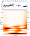 |
Fig. 1 Short-term Fourier transform of the dataset used in Sect. 3.1. A 10.7-12.1-year-long cycle is seen throughout the whole plot, and in the more recent half of the light curve, a 7.3-8.2-year-long period also appears. Features longer than 27 years are suppressed on the plot to one-third of the power. The peak in this range originates from the length of the available data and the gap between 1960 and 1970. |
3.2 Analytic spot model
We fit the light curve obtained from the long-cadence full-frame TESS images with an analytic three-spot model following the equations of Budding (1977) as implemented by Ribárik et al. (2003). The method uses circular spots that are allowed to overlap each other. Since the light curves showed clear signs of spot evolution, we applied time-series spot modeling: The time interval was divided into subintervals, and we fit a regular analytical model for each subinterval. This resulted in a set of spot parameters that were a function of time. The width of the time-series window was 1.25 Prot and the step size was 0.25 Prot, where the rotational period was kept at Prot = 2.606 d for the comparison with the Doppler maps. In the overlapping parts, we obtained the final theoretical brightnesses by averaging the theoretical brightnesses of each overlapping part (Bartus 1996). The Levenberg–Marquardt algorithm was applied during minimization.
Photometric starspot modeling is an inherently degenerate problem. Out of the four parameters that describe an analytic spot (i.e., spot latitude and longitude, spot temperature, and spot radius), only the longitude can be recovered reliably. The other three parameters are not independent and a greater change in the light curve can be caused by a cooler spot, a larger spot, or a different spot latitude depending on the inclination. We therefore chose a simplified modeling approach. During the fitting process, the spot latitudes were kept at 30◦ and the spot temperatures at 4600 K. These results were based the Doppler map of Järvinen et al. (2018). The umbral spot temperature difference for their most dominant spot is ∆T∼1000 K, which we applied to our rounded effective temperature derived from spectral synthesis (see Table 1). We note that we chose not to use our Doppler maps because spot temperatures can be distorted by the smearing effect of the lower resolution (see Appendix A and Kriskovics et al. 2023). The spot longitudes and the spot sizes were the free parameters of the fits. The rotational period used during the light-curve fitting was kept at the same constant value as used for the Doppler inversions.
Our seasonal period analysis shows clear signs of changes that indicate differential rotation or changing spot latitudes, or both. When all spot parameters were fit, however, the degeneracy of the problem often renders the interpretation and comparison of the spot parameters unreliable. Our approach made the comparison between Doppler maps and the photometric models clearer, and it also enabled us to carry out the analysis described in Sect. 3.3. These were our primary goals with the photometric spot modeling.
The fitting was carried out for the following sectors: S14, S15, S16, S21, S22, S23, S41, S48, S49, S50, S75, S76, and S77. The results are shown in Figs. 2 and B.1–B.3.
Stellar parameters of EK Dra.
3.3 Change in the spot longitudes
The shift in the spot longitudes in the middle panels of Figs. 2 and B.1–B.3 can be used to infer the operation of differential rotation. During a suitably chosen short interval, the longitude values of a spot with a rotation period different from the photometric period change with some slope compared to the horizontal. Based on the TESS light curves, it appears that each such interval is about 10–15 days, or roughly half a TESS sector. Within these intervals, the spots are considered stable, that is, spot evolution is disregarded. (We note here that all this is consistent with the Doppler images to be presented in Sect. 4.2.) The changes in spot longitude from photometric spot modeling within each time interval were approximated by a linear function, and by comparing the different slopes, we determined whether the spots rotated faster or slower than the photometric period. The average of the fit slopes is 1.3◦/d, and the standard deviation is 4.6◦/d. This spread in the slopes indicates differential rotation. A more thorough determination is not possible with this method, however. We would only be able to estimate the magnitude of the differential rotation if we knew the exact latitude coordinates of the spots. They can only be derived in photometric spot models with great uncertainty.
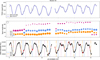 |
Fig. 2 TESS light curve of EK Dra from Sector 14 with the spot model. Top: light curve from the full-frame images (gray) and the three-spot-model fit (blue). Middle: change in spot longitudes. The sizes of the dots are scaled by the spot radii. Bottom: PDCSAP light curve along with the flares (red). The vertical lines indicate the times when the spots are in the line of sight. |
3.4 Change in the rotational period due to differential rotation
We determined the rotational period for consecutive TESS sectors (S14-16, S21-23, S41, S48-50, and S75-77) using a windowed Lomb-Scargle transform as implemented by Bódi (2024). The period uncertainty δP was calculated for the continuous observational windows from their obtained rotational period Prot and duration TN according to the relation δP ∼ Prot/TN. Figure 3 shows the results we obtained for each observation period. The average relative deviation of the rotational periods calculated from these is  , which can be a lower estimate of the surface differential rotation (relative shear) when we assume that the cause of the period change is primarily the differential rotation and the change in the latitudinal positions of the dominant spots (for previous applications of this photometric method, see, e.g., Berdyugina et al. 2002; Siltala et al. 2017; Kővári et al. 2021, 2025).
3.5 Flares
We investigated the flaring characteristics of EK Dra based on the PDCSAP light curves in the available 12 TESS sectors. The flares were individually collected by visual inspection of the PDCSAP light curves. We found 142 flares in this way. We note that the noise level of the light curve changes smoothly for most sectors, except for S76, where it increased abruptly. This hinders the detection of smaller flares in that sector, but we did not use a flare-finding algorithm that is directly tied to the photometric scatter, and we therefore estimate that its effect on the flare statistics is negligible.
In order to calculate the flare energies, we used the same approach as in Oláh et al. (2022) and Seli et al. (2025), described below. After marking the flaring data points and normalizing the light curves, we first fit fourth-order polynomials to the 30−30 minute light-curve segments bordering each individual flare on either side (Fig. 4). The baseline defined this way was removed as the next step. On the resulting data, we calculated the area below each flare (equivalent duration; ED) by integrating according to Simpson’s rule4. We integrated a BT-NextGen model spectrum (Hauschildt et al. 1999) with Teff=5700 K, log g=4.4 and solar metallicity over the entire wavelength range with and without convolving with the TESS response function to calculate the ratio of TESS (LTESS) to bolometric luminosity (Lbol). By applying the bolometric correction on the absolute magnitude using the method described by Creevey et al. (2023) and the data from Gaia Collaboration (2023), the value of Lbol was determined. With the above considerations, the flare energy in the TESS band was calculated as follows:
 (2)
(2)
The flare frequency distribution diagram (FFD) is shown in Fig. 5. At low energies, the flare events have a lower recovery rate due to the light curve noise, so that only flares with energies higher than E = 1033 erg were considered in the following analysis. (For a detailed flare injection test, see Kővári et al. 2020.) A breaking point around E = 1034 erg divided the FFD into two parts. The fit between E = 1033 erg and 1034 erg yielded a power-law index of 1.466 ± 0.007, and above E = 1034 erg yielded a power-law index of 2.335 ± 0.110.
We investigated the longitudinal distribution of flares by applying Kuiper’s test (Kuiper 1960) to our data to determine whether it comes from a uniform phase distribution. Unlike the similar Kolmogorov−Smirnov test, it is invariant under cyclic transformations, which makes it suitable for investigating the cyclic phase distribution. Based on this test, we cannot reject the null hypothesis of a uniform flare phase distribution. Because the starspots of EK Dra evolve quickly, however, it might be more suitable to compare the phase preference of flares to the spot locations.
To investigate whether the flares were associated with the active regions that cause the spot modulation observed in the TESS light curves, we propose a simple test. Using the results of the analytic three-spot model described in Sect. 3.2, we assigned each flare to the spot closest in longitude. We assume that the flare originated from the meridian, and we therefore used the phase of the flare mid-time to calculate its longitude. We then calculated the longitudinal difference between the flare and the closest spot and compared these differences to artificial distributions in which the same number of flares were distributed randomly in time. We used a two-sample Kolmogorov−Smirnov test to compare the observed distribution to the artificial distributions. After running 1000 tests with different random flare times, we were unable to reject the null hypothesis of a random flare phase occurrence (with a median p-value of 0.5). Because visible spots occur at every rotational phase, the assumption that the flares originate from the meridian is likely violated, which means that this simple test can only provide weak evidence of a random flare occurrence.
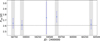 |
Fig. 3 Rotational periods of EK Dra (blue dots) and their estimated error bars in consecutive TESS observation windows (adjacent sectors are considered continuous). The gray areas from left to right are sectors S14-16, S21-23, S41, S48-50, and S75-77. The horizontal dashed line marks the rotation period value we adopted for the Doppler imaging. |
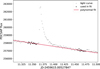 |
Fig. 4 Example of the polynomial fitting of the flare baseline. The data are marked in gray, the black points were used for the fit, and red shows the baseline fit. The flare is from Sector 48. |
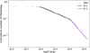 |
Fig. 5 Flare frequency distribution from TESS PDCSAP data. The black line denotes the fit with a power-law index of 1.466 ± 0.007 in the 1033–1034 erg energy range. The purple line is a fit above 1034 erg, and its power-law index is 2.335 ± 0.110. |
4 Spectroscopic analysis
4.1 Age
Carlos et al. (2016) found a strong correlation between the age of young solar analog stars and their lithium abundances. Using this empirical correlation and the lithium abundance from the result of our spectral synthesis (NLTE corrected value: A(Li)=2.28±0.04), we estimated the age of EK Dra to be t=0.070±0.018 Gyr. This reinforces the assumption that EK Dra is a young solar analog and agrees well with previous results (e.g. Güdel 2007).
4.2 Doppler imaging
4.2.1 Astrophysical parameters
Precise astrophysical parameters are required for successfully reconstructing the surface of a star through Doppler imaging. For this reason, we performed a spectroscopic analysis based on spectral synthesis using the code spectroscopy made easy (SME; Piskunov & Valenti 2017) with MARCS atmospheric models (Gustafsson et al. 2008) and atomic line parameters taken from the Vienna Atomic Line Database (VALD; Kupka et al. 1999). The value of the macroturbulence was estimated following the relation from Valenti & Fischer (2005),
 (3)
(3)
The final values of the astrophysical parameters were determined during an iterative process. The steps are listed below.
The initial astrophysical parameters were taken from Järvinen et al. (2018).
log g was fit using stronger lines (log g f > 0).
The effective temperature was fit using log g from the previous step.
Fit of the metallicity with a constant value of log g and Teff.
Fit of v sin i and vmic.
Refit of log g, Teff, and metallicity simultaneously to confirm robustness.
The results are summarized in Table 1 along with the other stellar parameters taken from the literature. These values were used for all of the Doppler inversions.
Temporal distribution of the datasets for each individual Doppler image.
4.2.2 The Doppler-imaging code iMap
The Doppler imaging was carried out with
iMap(Carroll et al. 2012). It performs multiline Doppler inversion using a list of user-provided photospheric lines. These relatively unblended lines were chosen from the 5000–7000 Å range and have a well-defined continuum and suitable temperature sensitivity. The lines in this list are referred to as “imaging lines”. The code uses a full radiative solver (Carroll et al. 2008) for every local line profile on the stellar surface that was divided into 5◦ × 5◦ segments. Atomic line data for the Doppler inversion were taken from VALD. The model atmosphere from Castelli & Kurucz (2003) was interpolated for the required temperature, gravity, and metallicity. Instead of a spherical model atmosphere, the code uses LTE radiative transfer, where the multiline approach compensates for the imperfections in the fit line shapes. The stellar parameters we used for the inversion are listed in Table 1. Finally, we note that during image reconstruction, no additional constraints were added because the surface reconstruction uses an iterative regularization method based on the Landweber algorithm (see Carroll et al. 2012).
4.2.3 Surface reconstruction and temporal variations
We observed more than 900 spectra during 30 months. These were divided into 13 subsets (DI01-DI13), and we selected from each of these subsets those with the highest S/N to cover the rotation phases. (Detailed information on the subsets can be found in Table 2 and Fig. C.1). In some cases, we included data with lower S/N to minimize the phase gaps between the spectra. This decreased the number of mapping lines (Table 2) in the case of three images because they were significantly contaminated by cosmics. The effect of all this does not appear on the quality of the Doppler reconstructions, however, because we usually used a robust average of 40 mapping lines from the optical range, compared to which, 30 or 35 are equally sufficient.
To facilitate referencing the consecutive Doppler images, we defined five observing runs (ORs) that included the following images: OR1 is DI01, OR2 is DI02-DI05, OR3 is DI06-DI07, OR4 is DI08-DI10, and OR5 is DI11-DI13. Figure 6 shows the resulting 13 Doppler images, and the corresponding line-profile fits are presented in Fig. C.2. In each of the maps, multiple low-latitude spots are visible with a temperature that is 700–1300 K lower than that of the unspotted stellar surface. OR1 consists of one image, and three spots are in phases ϕ∼0.2, ϕ∼0.55, and ϕ∼0.8. OR2 has the lowest spot temperatures and covers the longest time (55 days) of all the observing runs. Even though these recovered images are not consecutive, we treated them as one observing run. A spot is consistently visible at ϕ∼0.0. Because of the time gaps between maps, we cannot determine whether these are the same spot or if decay and emergence occurred between them. At ϕ∼0.25, a spot is present in the first three images, and it is the strongest in the second. The southernmost spots are at ϕ∼0.5. They appear around −30◦ latitude. Typically, Doppler maps show features on the more visible (upper) hemisphere due to reasons inherent to the method, but since it appears on multiple maps that were reconstructed from independent data, we argue that this is a real surface feature.
The time frame for OR3 was 12 days and contains DI06, which is the rotation with the widest phase gap. The spot configuration changed slightly between DI06 and DI07. The spot at ϕ∼0.85 became more prominent, and the two spots at ϕ∼0.15 and ϕ∼0.40 remained at about the same longitude. The feature in DI06 at ϕ∼0.7 coincides with the phase gap and is not visible in the following image, DI07. It is therefore mostly likely an artifact. Both OR4 and OR5 have three Doppler images covering two weeks of data. In the case of OR4, the spots at ϕ∼0.25 and ϕ∼0.5 became more prominent between DI08 and DI09, then weakened to DI10. The spot at ϕ∼0.0 was visible in DI08, but disappeared in later maps. In OR5, the spots at ϕ∼0.15 and ϕ∼0.35 diminish to DI13, while the spot at ϕ∼0.7 strengthens.
OR5 was planned to run parallel with TESS sector 77, but due to an unexpected gap in the photometric measurements, the two datasets only partially overlap. No flares can be observed on the light curve during the spectroscopic observations, so that the effects of these high-energy events in the spectra cannot be analyzed, even thought this was one of the original goals of OR5. On the other hand, the spot locations in the Doppler images and those obtained from the analytic three-spot model match well (spots at ϕ∼0.15, ϕ∼0.35, and ϕ∼0.7).
We note that the average temperature of the spots gradually decreased from OR2 to OR4 and slightly increased to OR5. The spot temperature change affects the average temperature of the stellar surface. This change can be quantified by the SME spectral analysis. To do this, we used spectra with a signal-to-noise ratio greater than 80. In the resulting Fig. 7, the black triangles mark the average for each DI. The spots cause a 69 ± 14 K variation in effective temperature.
With the limited spectral resolving power of R=21 000, approximately  resolution elements can be assumed across the stellar disk in our Doppler-images. Although the optimal would be at least twice this number, this is still acceptable given the circumstances (cf. Strassmeier et al. 2023). This is sufficiently supported by our previous tests (Kriskovics et al. 2023), with which we thoroughly explored the issue of moderate-resolution data (see also our further investigations in this regard in Appendix A). Finally, we mention that an insufficient coverage of the rotation phase by observations (i.e., long phase gaps) can cause artifacts in the Doppler images because the inversion lacks information about the phases that are not adequately covered by the observations (Cole-Kodikara et al. 2019). This is especially problematic when the phase gaps are longer than ∼0.25. Three of our images (DI04, DI05, and DI06) have a phase gap of this size, and the gaps in all others are below ∼0.2. iMap has been proven to be robust and reliable in handling occasional phase gaps (e.g. Järvinen et al. 2018; Kriskovics et al. 2024). Moreover, artifacts caused by phase gaps usually have a distinct shape, and we saw on only one such shape in our images.
We therefore consider the spatial resolution of our images to be moderate but acceptable, with negligible artifacts. This is also confirmed by our test results. Finally, the reliability of our images is also strengthened by the fact that Doppler maps that are within a given OR, that is, directly consecutive in time, but based on completely independent data, are highly similar (except for some traces of rapid spot evolution that occurred in the meantime).
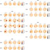 |
Fig. 6 Doppler images of EK Dra for the five observing runs. A total of 13 Doppler maps are displayed using the same temperature range. |
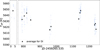 |
Fig. 7 Effective temperature from spectral synthesis for spectra with S/N higher than 80. The black triangles mark the average for each DI. The spots cause 68.7 ± 14.3 K variation in effective temperature. |
4.3 Differential rotation
The cross-correlation of Doppler images is a widely used method for measuring the surface differential rotation (Donati & Collier Cameron 1997). The evolution of spots (formation, dimming, and interaction) can make the result of this technique unstable. To counteract this, we made use of
ACCORD(e.g., Kővári et al. 2012, Kővári et al. 2015). The code uses the normalized average of the cross-correlations of consecutive Doppler images to measure differential rotation of the stellar surface by fitting the latitudinal cross-correlation peaks with a quadratic rotational law of the form
 (4)
where Ω(β) is the angular velocity at β latitude, and the dimensionless surface shear parameter αDR = (Ωeq − Ωpole)/Ωeq is calculated from the equatorial and polar angular velocities Ωeq and Ωpole, respectively. This quadratic approximation originally comes from solar physics (e.g. Beck 2000), but is widely used for spotted stars (see, e.g. Kővári et al. 2017, and their references).
(4)
where Ω(β) is the angular velocity at β latitude, and the dimensionless surface shear parameter αDR = (Ωeq − Ωpole)/Ωeq is calculated from the equatorial and polar angular velocities Ωeq and Ωpole, respectively. This quadratic approximation originally comes from solar physics (e.g. Beck 2000), but is widely used for spotted stars (see, e.g. Kővári et al. 2017, and their references).
In OR2, OR3, OR4, and OR5, we reconstructed consecutive maps of the stellar surface. These observing runs contained three, two, three, and three time-series Doppler images, respectively, that were suitable for the cross-correlation process detailed above. The resulting differential rotation parameter is αDR = 0.030 ± 0.008, and the fit is shown in Fig. 8. This average differential rotation has a visible effect over 8.943 days that might also be visible in our Doppler maps.
4.4 The variations in the Hα line
For each spectrum, we measured the Hα chromospheric activity indices (IHα) in order to examine the rotational modulation of the chromospheric activity. The method for obtaining these indices was the same as in Kürster et al. (2003). The line index is defined in a way that shows the change in the Hα line flux relative to the continuum flux,
 (5)
(5)
 is the mean spectral flux in the [−15.5, +15.5] km s−1 radial velocity interval centered on the core of the 6562.808 Å Hα line.
  and
and  are the mean fluxes from the [−700, −300] km s−1 and [+600, +1000] km s−1 radial velocity intervals, respectively.
By calculating the apparent average surface temperature of EK Dra over phases per thousand rotations, we recovered the temperature curve for each DI. Since the change in temperature is the consequence of stellar spots, the rotational modulation of the Hα chromospheric activity indicator can be directly compared to the spot distribution.
The resulting IHα and temperature curves (Fig. 9) show changes with the rotational phase. The Hα line is highly variable, and consequently, so is the scatter of the index. Most cases do not present a clear trend or anticorrelation with the temperature curve, which we would expect based on the solar analogy. In contrast, from 2020 data of EK Dra, Namekata et al. (2022a) found a clear overlap between the brightening in Hα and the brightness decrease in the TESS light curve caused by the associated spot group. Only DI03 of our Doppler images shows something similar: log IHα shows a raised value in the spot-covered phases, indicating that the most chromospherically active locations are above the stellar spots.
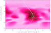 |
Fig. 8 Average cross-correlation function map for the consecutive Doppler reconstructions. The white circles mark the cross correlation peaks, and the continuous white line shows the quadratic differential rotational law we fit. The best-fit surface shear corresponds to αDR = 0.030 ± 0.008 shear coefficient and indicates a solar-type differential rotation. |
5 Discussion
5.1 Long-term photometry and cycles
The cyclic behavior of EK Dra was studied by Messina & Guinan (2002), who found a 9.2-year cycle. Later, Järvinen et al. (2018) refined this value to 8.9±0.2 years. The two studies made use of 20- and 30-year light curves, respectively (the periods overlapped), and also concluded that the star had continued to fade since 1985 until the end of the observations.
We studied the long-term photometric behavior of EK Dra based on the Sect. 2.1 light curve spanning over 120 years. The star shows a cyclic behavior with a period of 10.7–12.1 years, which reinforces the findings of the above-mentioned studies and shows that this cycle has been persistent for the past century. We found an additional cycle with a period of 7.3–8.2 years that appeared around 1950–1960. At this point, the star also began to dim, which persisted for about ∼64 years. Considering the preceding 60-year brightening phase, one possible interpretation of the data is a cycle longer than a century. However, this long-term brightening does not necessarily imply a cyclic variation, as pointed out by Oláh et al. (2014). A possible explanation for a magnetically driven noncyclic but trend-like long-term brightness change of the red giant XX Tri was recently suggested by Strassmeier et al. (2024). According to these authors, the continuously blocked flux by large cool starspots can be redistributed on a global scale rather than locally through an increase in, for example, facula activity. It thereby alters the overall brightness of the star on a timescale that is likely much longer than the stellar rotation, even over decades.
While the binary component might also be the cause of the long-term brightness variation, we argue that this is not the case here. Based on König et al. (2005), one periastron was at about 1987 and the previous one between 1937–1947. The earlier of these periastra occurred when the star was brightening, the other when it was dimming. These dates are well covered with data points, so that the different trends are clearly visible, and no similar change can be seen in the light curve at the two peri-astra. The STFT analysis cannot detect the periodicity caused by the binary component because the possible STFT peak by the binary period overlaps the peak caused by the gap in the data; both result in a peak at a period of ∼50 years, which makes the two undistinguishable.
In order to place the activity cycles of EK Dra in the context of other active stars, we show in Fig. 10 the Prot rotational and Pcyc cycle periods from Oláh et al. (2009) and Oláh et al. (2016), plot the relation between Pcyc/Prot and 1/Prot, and include EK Dra in the sample. The cycles derived for EK Dra are consistent with those of fast rotators.
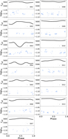 |
Fig. 9 Variation in the Hα index (described in Sect. 4.4) compared to the change in effective temperature. |
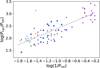 |
Fig. 10 Relation between rotational and cycle periods. The cycles we obtained from the long-term photometry data for EK Dra are marked by red diamonds. The cycles for stars denoted in purple are taken from Oláh et al. (2009). The rest are adopted from Oláh et al. (2016), who distinguished between simple cycles (light blue circles), complex cycles (dark blue squares), and additional cycles (black dots) to the complex ones. The solar cycles (Gleissberg, Schwabe, and 3–4-yr cycles) are marked in orange. |
5.2 Flare activity
The flare energy distribution of EK Dra can be described by a broken power law. The Sun (Kasinsky & Sotnicova 2003) and some dwarf stars (Paudel et al. 2018) shows the same behavior. This break in the power law might be caused by statistical fluctuations. At the same time, the breaking point was interpreted by Mullan & Paudel (2018) as a critical energy above which the size of the magnetic loop, which becomes twisted and releases its energy in the shape of flares, becomes higher than the local scale height. This critical energy is changing from one star to the next, and for EK Dra, it is about E = 1034 erg. We derived a power-law index of 1.466 ± 0.007 below this energy. Namekata et al. (2022a) conducted a similar analysis for TESS sectors 14–16 and 21–23. The slope of our FFD between E = 1033 and E = 1034 matches theirs within the errors.
In Sect. 3.5 we investigated the longitudinal flare distribution and compared the distribution of flares to that of the spots by applying the Kuiper test and the two-sample Kolmogorov−Smirnov test, respectively. Neither of the cases can reject the null hypothesis of a uniform flare distribution.
5.3 Spot activity and differential rotation
From one rotation to the next, the spot configuration on the surface of EK Dra changes. This variation was modeled with an analytic three-spot model (Figs. 2, B.1, B.2, B.3) and appears as the decay and emergence of spots, as well as their shift in position. The deviation of the analytic model from the light curve can be attributed to either smaller spots or to the spots being approximated with perfect circles during the modeling. In addition, the longitudinal positions of the spots, which can be derived relatively precisely from photometric spot models, show trend-like changes that suggest that the stellar surface rotates differentially.
The surface changes of EK Dra on the rotational timescale can also be confirmed with the Doppler images (Fig. 6), especially with those that are immediately consecutive in time. The reconstructed spots appear mostly at mid-latitudes, around 30-60◦, but they also appear at low latitudes, and a few cross the equator (see, e.g., DI12). The numerical simulation of the flux emergence (Schuessler et al. 1996; Granzer et al. 2000; Iʂık et al. 2018) was unable to reproduce these low-latitude spots and thus predicted a zone of avoidance between ±20◦. Şenavci et al. (2021) found that information on activity in the less visible hemisphere at mid-latitudes can leak and cause these low-latitude spots. Unlike these, the flux emergence simulation in Iʂık et al. (2024) reinforces the hypothesis that these spots are real surface features on fast-rotating solar-type stars. The variation in the surface also appears in the effective surface temperature obtained by SME (Fig. 7). The spots cause a 69±14 K variation in effective temperature. We note that the relatively low resolution of our instrument affects the result of the Doppler inversion. This is tested and discussed in Appendix A.
EK Dra has a long history of Doppler imaging. The first such study was carried out by Strassmeier & Rice (1998), and ever since, multiple Doppler images were obtained (e.g. Järvinen et al. 2007; Waite et al. 2017; Järvinen et al. 2018; Namekata et al. 2024). These studies analyzed one to four maps, while our campaign reconstructed 13 images with multiple consecutive maps. This provides an opportunity to follow the short-term changes on the surface and to recover the differential rotation shear parameter αDR = 0.030±0.008. Figure 11 shows that this value obtained for EK Dra fits the trend observed for stars with different rotational periods. We note that earlier attempts were made to recover the differential rotation parameter, and the resulting values were lower by an order of magnitude (αDR = 0.00091 ± 0.00001; Järvinen et al. 2007) or higher (αDR = 0.108 ± 0.0554; Waite et al. 2017) than ours.
Linear and nonlinear spot decay models (e.g., Petrovay & van Driel-Gesztelyi 1997; Muraközy 2021) originate from the observational fact that the lifetimes of sunspots depend on their area. In decay models, the spots on EK Dra can either be considered as monolithic spots or as clusters of smaller spots because the resolution of our Doppler imaging does not reach the typical size of sunspots. Based on the Doppler maps, the lower limit for the lifetime of stellar spots is about 10–15 days. Kővári et al. (2024) reported a similar value in the V815 Her system for the Aa component, which is a 30 Myr solar analog. Iʂik et al. (2007) found that while large monolithic spots have a lifetime of months, a cluster of small spots decays on a timescale of a few days to a few dozen days. Although the lifetime of the spots on EK Dra matches that of the spot clusters better, Järvinen et al. (2018) found no evidence of a conglomerate like this. Namekata et al. (2019) reported that the spots on rapidly rotating stars evolve on a shorter timescale, so that the rotational period of EK Dra might be one of the key factors in the lifetime of its spots.
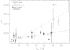 |
Fig. 11 Absolute value of the surface shear coefficient αDR as a function of the rotational period for spotted stars (Kővári et al. 2017). Single stars are indicated by circles, and those in binary systems are denoted by filled symbols. EK Dra is marked in red. The dotted line shows a linear fit to single stars with a slope of |αDR| ∝ 0.0049 Prot[d], the lower slope of the dash-dotted line is |αDR| ∝ 0.0014 Prot[d], and it is fit to stars in binary systems (Kriskovics et al. 2023). |
6 Conclusions
We used photometric and spectroscopic data from the young solar analog EK Dra to investigate the magnetic activity of the star on shorter and longer timescales. We summarize our main conclusions below.
From long-term photometric data, we found that EK Dra exhibits a 10.7−12.1 year cycle that was persistently present for 120 years. In addition, the star shows a 60 years-long dimming phase preceded by a brightening phase, which indicates a possible cycle period longer than 120 years.
We modeled light curves from 13 TESS sectors using an analytical three-spot model. From the longitudinal shifts of the spots, we infer a surface differential rotation.
We found a total of 142 flares in the TESS data. Their longitudinal distribution is not correlated with the rotational phase or with the spotted longitudes. The flare energy distribution follows a broken power law with indices 1.466 ± 0.0007 for the E = 1033−1034 erg range and 2.335 ± 0.11 above E = 1034 erg.
The 13 reconstructed Doppler images show that the spotted surface of EK Dra varies from one rotation to the next, and the lifetime of the spots is 10–15 days.
Consistent with the differential rotation suggested by the photometric spot modeling, the Doppler imaging showed that the star exhibits solar-type differential rotation with a surface shear parameter of αDR = 0.030 ± 0.008. This value, obtained by cross-correlation of consecutive Doppler images, agrees well with the
 value, which is a rough estimate of the shear parameter from the rotation period changes.
The Hα line was shown to be highly variable, and the derived activity indices therefore have a large scatter. This makes the connection between photospheric and chromospheric activity inconclusive.
Further photometric observations might confirm the long-term brightening and dimming as part of an activity cycle or as a change related to the evolution of EK Dra. Moreover, the relation between the photosphere and the chromosphere is also a subject of further research: As we showed for EK Dra, chromospheric tracers are not always closely associated with the photospheric spots.
Acknowledgements
The authors thank the anonymous referee for improving the quality of the paper with helpful comments and suggestions. This research was funded by the Hungarian National Research, Development and Innovation Office grant Élvonal KKP-143986. Authors acknowledge the financial support of the Austrian-Hungarian Action Foundation grants 98öu5, 101öu13, 104öu2, 112öu1. L.K. acknowledges the support of the Hungarian National Research, Development and Innovation Office grant PD-134784. K.V. is supported by the Bolyai János Research Scholarship of the Hungarian Academy of Sciences. On behalf of the “Looking for stellar CMEs on different wavelengths” project we are grateful for the possibility of using HUN-REN Cloud Héder et al. (2022) which helped us achieve the results published in this paper. This work has used data provided by Digital Access to a Sky Century @ Harvard (DASCH), which has been partially supported by NSF grants AST-0407380, AST-0909073, and AST-1313370. This paper includes data collected by the TESS mission. Funding for the TESS mission is provided by the NASA’s Science Mission Directorate.
References
- Bartus, J. 1996, Konkoly Observ. Occasional Tech. Notes, 6, 1 [Google Scholar]
- Beck, J. G. 2000, Sol. Phys., 191, 47 [NASA ADS] [CrossRef] [Google Scholar]
- Berdyugina, S. V., Pelt, J., & Tuominen, I. 2002, A&A, 394, 505 [NASA ADS] [CrossRef] [EDP Sciences] [Google Scholar]
- Bódi, A. 2024, J. Open Source Softw., 9, 7118 [Google Scholar]
- Brahm, R., Jordán, A., & Espinoza, N. 2017, PASP, 129, 034002 [Google Scholar]
- Budding, E. 1977, Ap & SS, 48, 207 [Google Scholar]
- Cappelli, A., Cerruti-Sola, M., Cheng, C. C., & Pallavicini, R. 1989, A&A, 213, 226 [Google Scholar]
- Carlos, M., Nissen, P. E., & Meléndez, J. 2016, A&A, 587, A100 [NASA ADS] [CrossRef] [EDP Sciences] [Google Scholar]
- Carroll, T. A., Kopf, M., & Strassmeier, K. G. 2008, A&A, 488, 781 [NASA ADS] [CrossRef] [EDP Sciences] [Google Scholar]
- Carroll, T. A., Strassmeier, K. G., Rice, J. B., & Künstler, A. 2012, A&A, 548, A95 [NASA ADS] [CrossRef] [EDP Sciences] [Google Scholar]
- Castelli, F., & Kurucz, R. L. 2003, IAU Symp., 210, A20 [Google Scholar]
- Chugainov, P. F., Lovkaya, M. N., & Zajtseva, G. V. 1991, Inform. Bull. Variab. Stars, 3680, 1 [Google Scholar]
- Cole-Kodikara, E. M., Käpylä, M. J., Lehtinen, J. J., et al. 2019, A&A, 629, A120 [NASA ADS] [CrossRef] [EDP Sciences] [Google Scholar]
- Creevey, O. L., Sordo, R., Pailler, F., et al. 2023, A&A, 674, A26 [NASA ADS] [CrossRef] [EDP Sciences] [Google Scholar]
- Donati, J. F., & Collier Cameron, A. 1997, MNRAS, 291, 1 [NASA ADS] [CrossRef] [Google Scholar]
- Gaia Collaboration (Vallenari, A., et al.) 2023, A&A, 674, A1 [NASA ADS] [CrossRef] [EDP Sciences] [Google Scholar]
- Granzer, T., Schüssler, M., Caligari, P., & Strassmeier, K. G. 2000, A&A, 355, 1087 [NASA ADS] [Google Scholar]
- Grindlay, J., Tang, S., Los, E., & Servillat, M. 2012, IAU Symp., 285, 29 [Google Scholar]
- Güdel, M. 2004, A&A Rev., 12, 71 [Google Scholar]
- Güdel, M. 2007, Liv. Rev. Sol. Phys., 4, 3 [Google Scholar]
- Gustafsson, B., Edvardsson, B., Eriksson, K., et al. 2008, A&A, 486, 951 [NASA ADS] [CrossRef] [EDP Sciences] [Google Scholar]
- Hauschildt, P. H., Allard, F., & Baron, E. 1999, ApJ, 512, 377 [Google Scholar]
- Héder, M., Rigó, E., Medgyesi, D., et al. 2022, Információs Társadalom, 22, 128 [Google Scholar]
- Iʂik, E., Schüssler, M., & Solanki, S. K. 2007, A&A, 464, 1049 [NASA ADS] [CrossRef] [EDP Sciences] [Google Scholar]
- Iʂık, E., Solanki, S. K., Krivova, N. A., & Shapiro, A. I. 2018, A&A, 620, A177 [CrossRef] [EDP Sciences] [Google Scholar]
- Iʂık, E., Solanki, S. K., Cameron, R. H., & Shapiro, A. I. 2024, ApJ, 976, 215 [Google Scholar]
- Järvinen, S. P., Berdyugina, S. V., Korhonen, H., Ilyin, I., & Tuominen, I. 2007, A&A, 472, 887 [NASA ADS] [CrossRef] [EDP Sciences] [Google Scholar]
- Järvinen, S. P., Strassmeier, K. G., Carroll, T. A., Ilyin, I., & Weber, M. 2018, A&A, 620, A162 [NASA ADS] [CrossRef] [EDP Sciences] [Google Scholar]
- Jenkins, J. M., Twicken, J. D., McCauliff, S., et al. 2016, SPIE, 9913, 99133E [NASA ADS] [Google Scholar]
- Kasinsky, V. V., & Sotnicova, R. T. 2003, Astron. Astrophys. Trans., 22, 325 [Google Scholar]
- Kővári, Zs., Korhonen, H., Kriskovics, L., et al. 2012, A&A, 539, A50 [NASA ADS] [CrossRef] [EDP Sciences] [Google Scholar]
- Kővári, Zs., Kriskovics, L., Künstler, A., et al. 2015, A&A, 573, A98 [NASA ADS] [CrossRef] [EDP Sciences] [Google Scholar]
- Kővári, Zs., Oláh, K., Kriskovics, L., et al. 2017, Astron. Nachr., 338, 903 [Google Scholar]
- Kővári, Zs., Oláh, K., Günther, M. N., et al. 2020, A&A, 641, A83 [EDP Sciences] [Google Scholar]
- Kővári, Zs., Kriskovics, L., Oláh, K., et al. 2021, A&A, 650, A158 [NASA ADS] [CrossRef] [EDP Sciences] [Google Scholar]
- Kővári, Zs., Strassmeier, K. G., Kriskovics, L., et al. 2024, A&A, 684, A94 [NASA ADS] [CrossRef] [EDP Sciences] [Google Scholar]
- Kővári, Zs., Strassmeier, K. G., Oláh, K., et al. 2025, A&A, 701, A103 [NASA ADS] [CrossRef] [EDP Sciences] [Google Scholar]
- Kochukhov, O., Hackman, T., Lehtinen, J. J., & Wehrhahn, A. 2020, A&A, 635, A142 [NASA ADS] [CrossRef] [EDP Sciences] [Google Scholar]
- Kolláth, Z., & Oláh, K. 2009, A&A, 501, 695 [NASA ADS] [CrossRef] [EDP Sciences] [Google Scholar]
- König, B., Guenther, E. W., Woitas, J., & Hatzes, A. P. 2005, A&A, 435, 215 [NASA ADS] [CrossRef] [EDP Sciences] [Google Scholar]
- Kraft, R. P. 1967, ApJ, 150, 551 [Google Scholar]
- Kriskovics, L., Kővári, Zs., Seli, B., et al. 2023, A&A, 674, A143 [NASA ADS] [CrossRef] [EDP Sciences] [Google Scholar]
- Kriskovics, L., Kővári, Zs., Seli, B., et al. 2024, IAU Symp., 365, 70 [Google Scholar]
- Kuiper, N. H. 1960, Nederl. Akad. Wetensch. Proc. Ser. A, 63, 38 [CrossRef] [Google Scholar]
- Kupka, F., Piskunov, N., Ryabchikova, T. A., Stempels, H. C., & Weiss, W. W. 1999, A&AS, 138, 119 [Google Scholar]
- Kürster, M., Endl, M., Rouesnel, F., et al. 2003, A&A, 403, 1077 [NASA ADS] [CrossRef] [EDP Sciences] [Google Scholar]
- Lammer, H., Selsis, F., Ribas, I., et al. 2003, ApJ, 598, L121 [Google Scholar]
- Laycock, S., Tang, S., Grindlay, J., et al. 2010, AJ, 140, 1062 [NASA ADS] [CrossRef] [Google Scholar]
- Messina, S., & Guinan, E. F. 2002, A&A, 393, 225 [NASA ADS] [CrossRef] [EDP Sciences] [Google Scholar]
- Mullan, D. J., & Paudel, R. R. 2018, ApJ, 854, 14 [NASA ADS] [CrossRef] [Google Scholar]
- Muraközy, J. 2021, ApJ, 908, 133 [Google Scholar]
- Namekata, K., Maehara, H., Notsu, Y., et al. 2019, ApJ, 871, 187 [NASA ADS] [CrossRef] [Google Scholar]
- Namekata, K., Maehara, H., Honda, S., et al. 2022a, ApJ, 926, L5 [CrossRef] [Google Scholar]
- Namekata, K., Maehara, H., Honda, S., et al. 2022b, Nat. Astron., 6, 241 [NASA ADS] [CrossRef] [Google Scholar]
- Namekata, K., Ikuta, K., Petit, P., et al. 2024, ApJ, 976, 255 [Google Scholar]
- Noyes, R. W., Hartmann, L. W., Baliunas, S. L., Duncan, D. K., & Vaughan, A. H. 1984, ApJ, 279, 763 [Google Scholar]
- Oláh, K., Kolláth, Z., Granzer, T., et al. 2009, A&A, 501, 703 [NASA ADS] [CrossRef] [EDP Sciences] [Google Scholar]
- Oláh, K., Moór, A., Kővári, Zs., et al. 2014, A&A, 572, A94 [NASA ADS] [CrossRef] [EDP Sciences] [Google Scholar]
- Oláh, K., Kővári, Zs., Petrovay, K., et al. 2016, A&A, 590, A133 [NASA ADS] [CrossRef] [EDP Sciences] [Google Scholar]
- Oláh, K., Seli, B., Kővári, Zs., Kriskovics, L., & Vida, K. 2022, A&A, 668, A101 [NASA ADS] [CrossRef] [EDP Sciences] [Google Scholar]
- Pál, A. 2012, MNRAS, 421, 1825 [Google Scholar]
- Paudel, R. R., Gizis, J. E., Mullan, D. J., et al. 2018, ApJ, 858, 55 [Google Scholar]
- Petrovay, K., & van Driel-Gesztelyi, L. 1997, Sol. Phys., 176, 249 [Google Scholar]
- Piskunov, N., & Valenti, J. A. 2017, A&A, 597, A16 [NASA ADS] [CrossRef] [EDP Sciences] [Google Scholar]
- Ribárik, G., Oláh, K., & Strassmeier, K. G. 2003, Astron. Nachr., 324, 202 [CrossRef] [Google Scholar]
- Ribas, I., Guinan, E. F., Güdel, M., & Audard, M. 2005, ApJ, 622, 680 [Google Scholar]
- Ricker, G. R., Winn, J. N., Vanderspek, R., et al. 2015, J. Astron. Teles. Instrum. Syst., 1, 014003 [Google Scholar]
- Schuessler, M., Caligari, P., Ferriz-Mas, A., Solanki, S. K., & Stix, M. 1996, A&A, 314, 503 [Google Scholar]
- Seli, B., Vida, K., Oláh, K., et al. 2025, A&A, 694, A161 [NASA ADS] [CrossRef] [EDP Sciences] [Google Scholar]
- Şenavci, H. V., Kılıçoğlu, T., Iʂık, E., et al. 2021, MNRAS, 502, 3343 [NASA ADS] [CrossRef] [Google Scholar]
- Siltala, L., Jetsu, L., Hackman, T., et al. 2017, Astron. Nachr., 338, 453 [NASA ADS] [CrossRef] [Google Scholar]
- Simcoe, R. J., Grindlay, J. E., Los, E. J., et al. 2006, SPIE Conf. Ser., 6312, 631217 [Google Scholar]
- Skumanich, A. 1972, ApJ, 171, 565 [Google Scholar]
- Soderblom, D. R. 1985, AJ, 90, 2103 [NASA ADS] [CrossRef] [Google Scholar]
- Strassmeier, K. G., & Rice, J. B. 1998, A&A, 330, 685 [NASA ADS] [Google Scholar]
- Strassmeier, K. G., Boyd, L. J., Epand, D. H., & Granzer, T. 1997, PASP, 109, 697 [NASA ADS] [CrossRef] [Google Scholar]
- Strassmeier, K. G., Carroll, T. A., & Ilyin, I. V. 2023, A&A, 674, A118 [NASA ADS] [CrossRef] [EDP Sciences] [Google Scholar]
- Strassmeier, K. G., Kővári, Zs., Weber, M., & Granzer, T. 2024, Nat. Commun., 15, 9986 [Google Scholar]
- Tang, S., Grindlay, J., Los, E., & Servillat, M. 2013, PASP, 125, 857 [NASA ADS] [CrossRef] [Google Scholar]
- Valenti, J. A., & Fischer, D. A. 2005, ApJS, 159, 141 [Google Scholar]
- Vida, K., Kővári, Zs., Pál, A., Oláh, K., & Kriskovics, L. 2017, ApJ, 841, 124 [NASA ADS] [CrossRef] [Google Scholar]
- Vida, K., Oláh, K., Kővári, Zs., et al. 2019, ApJ, 884, 160 [NASA ADS] [CrossRef] [Google Scholar]
- Vida, K., Kővári, Zs., Leitzinger, M., et al. 2024, Universe, 10, 313 [Google Scholar]
- Vidotto, A. A., Gregory, S. G., Jardine, M., et al. 2014, MNRAS, 441, 2361 [Google Scholar]
- Waite, I. A., Marsden, S. C., Carter, B. D., et al. 2017, MNRAS, 465, 2076 [Google Scholar]
Astronomical Consultants & Equipment.
scipy.integrate.simps
Appendix A Comparison with PEPSI data and the effect of spectral resolution
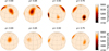 |
Fig. A.1 Doppler images of EK Dra using the dataset published in Järvinen et al. (2018). Top: Map with the resolution and inversion parameters used in Järvinen et al. (2018). Bottom: Map with the resolution downgraded to 20 000 and done with the inversion parameters from this paper. |
In addition to the Piszkéstető observations, the spectra published in Järvinen et al. (2018) were used for validation purposes. Using the method detailed in Kriskovics et al. (2023) the R = 230 000 ± 30 000 resolution PEPSI spectra were downgraded to R = 20 000 before Doppler imaging. In the resulting map (Fig. A.1), the location of the spots matches that of Järvinen et al. (2018). However, it is apparent that small-scale structures are suppressed by the lower resolution; the smallest spot reconstructed from the original PEPSI data at ϕ∼0.5, with an area of 3% and a temperature difference of ∆T = 280 K cannot be recovered after the resolution degradation. The shape of larger structures is somewhat simplified and the temperature contrast decreases with decreasing resolution, but their position is preserved and Doppler reconstructions are still suitable for studying short- and long-term spot evolution. Moreover, by averaging cross-correlation function maps of consecutive pairs of Doppler images, surface differential rotation can also be detected, as demonstrated by the tests of Kriskovics et al. (2023). We note that despite the lower resolution, short-term spot evolution and the gradual change of spot temperatures are clearly visible on the subsequent maps in Fig. 6. Finally we also mention that the reliability of our Doppler reconstructions is supported by the agreement between our DI08 image and the analytical three-spot model obtained for the temporally coincident TESS S77 data (cf. Figs. 6 and B.3).
Appendix B Analytic spot model for all available TESS sectors
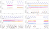 |
Fig. B.3 Same as Fig. 2 but for TESS sectors S75, S76, and S77. In the plot corresponding to Sector 77, the top panel shows the time of the spectrum measurements marked with red. For Sector 50 no TESS PDCSAP flux is available. |
Appendix C Line profile fits and phase distribution
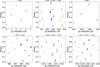 |
Fig. C.1 Phase distribution-optimized compilation of data subsets DI01-DI13 for Doppler imaging; cf. Table 2. |
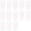 |
Fig. C.2 Line profile fits in the case of each DI. The black lines are the average line profiles of the imaging lines at a given phase, while the fitted profile is marked in red. |
All Tables
All Figures
|
Fig. 1 Short-term Fourier transform of the dataset used in Sect. 3.1. A 10.7-12.1-year-long cycle is seen throughout the whole plot, and in the more recent half of the light curve, a 7.3-8.2-year-long period also appears. Features longer than 27 years are suppressed on the plot to one-third of the power. The peak in this range originates from the length of the available data and the gap between 1960 and 1970. |
| In the text | |
|
Fig. 2 TESS light curve of EK Dra from Sector 14 with the spot model. Top: light curve from the full-frame images (gray) and the three-spot-model fit (blue). Middle: change in spot longitudes. The sizes of the dots are scaled by the spot radii. Bottom: PDCSAP light curve along with the flares (red). The vertical lines indicate the times when the spots are in the line of sight. |
| In the text | |
|
Fig. 3 Rotational periods of EK Dra (blue dots) and their estimated error bars in consecutive TESS observation windows (adjacent sectors are considered continuous). The gray areas from left to right are sectors S14-16, S21-23, S41, S48-50, and S75-77. The horizontal dashed line marks the rotation period value we adopted for the Doppler imaging. |
| In the text | |
|
Fig. 4 Example of the polynomial fitting of the flare baseline. The data are marked in gray, the black points were used for the fit, and red shows the baseline fit. The flare is from Sector 48. |
| In the text | |
|
Fig. 5 Flare frequency distribution from TESS PDCSAP data. The black line denotes the fit with a power-law index of 1.466 ± 0.007 in the 1033–1034 erg energy range. The purple line is a fit above 1034 erg, and its power-law index is 2.335 ± 0.110. |
| In the text | |
|
Fig. 6 Doppler images of EK Dra for the five observing runs. A total of 13 Doppler maps are displayed using the same temperature range. |
| In the text | |
|
Fig. 7 Effective temperature from spectral synthesis for spectra with S/N higher than 80. The black triangles mark the average for each DI. The spots cause 68.7 ± 14.3 K variation in effective temperature. |
| In the text | |
|
Fig. 8 Average cross-correlation function map for the consecutive Doppler reconstructions. The white circles mark the cross correlation peaks, and the continuous white line shows the quadratic differential rotational law we fit. The best-fit surface shear corresponds to αDR = 0.030 ± 0.008 shear coefficient and indicates a solar-type differential rotation. |
| In the text | |
|
Fig. 9 Variation in the Hα index (described in Sect. 4.4) compared to the change in effective temperature. |
| In the text | |
|
Fig. 10 Relation between rotational and cycle periods. The cycles we obtained from the long-term photometry data for EK Dra are marked by red diamonds. The cycles for stars denoted in purple are taken from Oláh et al. (2009). The rest are adopted from Oláh et al. (2016), who distinguished between simple cycles (light blue circles), complex cycles (dark blue squares), and additional cycles (black dots) to the complex ones. The solar cycles (Gleissberg, Schwabe, and 3–4-yr cycles) are marked in orange. |
| In the text | |
|
Fig. 11 Absolute value of the surface shear coefficient αDR as a function of the rotational period for spotted stars (Kővári et al. 2017). Single stars are indicated by circles, and those in binary systems are denoted by filled symbols. EK Dra is marked in red. The dotted line shows a linear fit to single stars with a slope of |αDR| ∝ 0.0049 Prot[d], the lower slope of the dash-dotted line is |αDR| ∝ 0.0014 Prot[d], and it is fit to stars in binary systems (Kriskovics et al. 2023). |
| In the text | |
|
Fig. A.1 Doppler images of EK Dra using the dataset published in Järvinen et al. (2018). Top: Map with the resolution and inversion parameters used in Järvinen et al. (2018). Bottom: Map with the resolution downgraded to 20 000 and done with the inversion parameters from this paper. |
| In the text | |
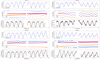 |
Fig. B.1 Same as Fig. 2 but for TESS sectors S15, S16, S21, and S22. |
| In the text | |
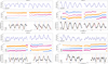 |
Fig. B.2 Same as Fig. 2 but for TESS sectors S23, S41, S48, and S49. |
| In the text | |
|
Fig. B.3 Same as Fig. 2 but for TESS sectors S75, S76, and S77. In the plot corresponding to Sector 77, the top panel shows the time of the spectrum measurements marked with red. For Sector 50 no TESS PDCSAP flux is available. |
| In the text | |
|
Fig. C.1 Phase distribution-optimized compilation of data subsets DI01-DI13 for Doppler imaging; cf. Table 2. |
| In the text | |
|
Fig. C.2 Line profile fits in the case of each DI. The black lines are the average line profiles of the imaging lines at a given phase, while the fitted profile is marked in red. |
| In the text | |
Current usage metrics show cumulative count of Article Views (full-text article views including HTML views, PDF and ePub downloads, according to the available data) and Abstracts Views on Vision4Press platform.
Data correspond to usage on the plateform after 2015. The current usage metrics is available 48-96 hours after online publication and is updated daily on week days.
Initial download of the metrics may take a while.