| Issue |
A&A
Volume 706, February 2026
|
|
|---|---|---|
| Article Number | A27 | |
| Number of page(s) | 20 | |
| Section | Astrophysical processes | |
| DOI | https://doi.org/10.1051/0004-6361/202557022 | |
| Published online | 28 January 2026 | |
Probing jet base emission of M87* with the 2021 Event Horizon Telescope observations
1
Max-Planck-Institut für Radioastronomie Auf dem Hügel 69 D-53121 Bonn, Germany
2
Jansky Fellow of National Radio Astronomy Observatory 1011 Lopezville Rd Socorro NM 87801, USA
3
Canadian Institute for Theoretical Astrophysics, University of Toronto 60 St. George Street Toronto ON M5S 3H8, Canada
4
Center for Astrophysics | Harvard & Smithsonian 60 Garden Street Cambridge MA 02138, USA
5
Black Hole Initiative at Harvard University 20 Garden Street Cambridge MA 02138, USA
6
Department of Astrophysics, Institute for Mathematics, Astrophysics and Particle Physics (IMAPP), Radboud University P.O. Box 9010 6500 GL Nijmegen, The Netherlands
7
Perimeter Institute for Theoretical Physics 31 Caroline Street North Waterloo ON N2L 2Y5, Canada
8
Department of Physics and Astronomy, University of Waterloo 200 University Avenue West Waterloo ON N2L 3G1, Canada
9
Waterloo Centre for Astrophysics, University of Waterloo Waterloo ON N2L 3G1, Canada
10
Steward Observatory and Department of Astronomy, University of Arizona 933 N. Cherry Ave. Tucson AZ 85721, USA
11
Institut für Theoretische Physik, Goethe-Universität Frankfurt Max-von-Laue-Straße 1 D-60438 Frankfurt am Main, Germany
12
Mizusawa VLBI Observatory, National Astronomical Observatory of Japan, 2-12 Hoshigaoka Mizusawa Oshu Iwate 023-0861, Japan
13
Astronomy Department, Universidad de Concepción Casilla 160-C Concepción, Chile
14
School of Space Research, Kyung Hee University, 1732, Deogyeong-daero Giheung-gu Yongin-si Gyeonggi-do 17104, Republic of Korea
15
Institute of Astronomy and Astrophysics, Academia Sinica, 11F of Astronomy-Mathematics Building, AS/NTU No. 1, Sec. 4 Roosevelt Rd. Taipei 106216, Taiwan, ROC
16
Instituto de Astrofísica de Andalucía-CSIC Glorieta de la Astronomía s/n E-18008 Granada, Spain
17
Massachusetts Institute of Technology Haystack Observatory 99 Millstone Road Westford MA 01886, USA
18
National Astronomical Observatory of Japan 2-21-1 Osawa Mitaka Tokyo 181-8588, Japan
19
Departament d’Astronomia i Astrofísica, Universitat de València C. Dr. Moliner 50 E-46100 Burjassot València, Spain
20
Department of Physics, Faculty of Science, Universiti Malaya 50603 Kuala Lumpur, Malaysia
21
Department of Physics & Astronomy, The University of Texas at San Antonio, One UTSA Circle San Antonio TX 78249, USA
22
Physics & Astronomy Department, Rice University Houston TX 77005-1827, USA
23
Observatori Astronòmic, Universitat de València C. Catedrático José Beltrán 2 E-46980 Paterna València, Spain
24
Department of Space, Earth and Environment, Chalmers University of Technology, Onsala Space Observatory SE-43992 Onsala, Sweden
25
Yale Center for Astronomy & Astrophysics, Yale University 52 Hillhouse Avenue New Haven CT 06511, USA
26
Department of Physics, University of Illinois 1110 West Green Street Urbana IL 61801, USA
27
Fermi National Accelerator Laboratory MS209 P.O. Box 500 Batavia IL 60510, USA
28
Department of Astronomy and Astrophysics, University of Chicago 5640 South Ellis Avenue Chicago IL 60637, USA
29
East Asian Observatory 660 N. A’ohoku Place Hilo HI 96720, USA
30
James Clerk Maxwell Telescope (JCMT) 660 N. A’ohoku Place Hilo HI 96720, USA
31
California Institute of Technology 1200 East California Boulevard Pasadena CA 91125, USA
32
Institute of Astronomy and Astrophysics, Academia Sinica 645 N. A’ohoku Place Hilo HI 96720, USA
33
Department of Physics and Astronomy, University of Hawaii at Manoa 2505 Correa Road Honolulu HI 96822, USA
34
Institut de Radioastronomie Millimétrique (IRAM), 300 rue de la Piscine F-38406 Saint Martin d’Hères, France
35
Department of Astronomy, University of Massachusetts Amherst MA 01003, USA
36
Instituto de Astronomia, Geofísica e Ciências Atmosféricas, Universidade de São Paulo, R. do Matão 1226 São Paulo SP 05508-090, Brazil
37
Kavli Institute for Cosmological Physics, University of Chicago 5640 South Ellis Avenue Chicago IL 60637, USA
38
Department of Physics, University of Chicago 5720 South Ellis Avenue Chicago IL 60637, USA
39
Enrico Fermi Institute, University of Chicago 5640 South Ellis Avenue Chicago IL 60637, USA
40
Princeton Gravity Initiative, Jadwin Hall, Princeton University Princeton NJ 08544, USA
41
Data Science Institute, University of Arizona 1230 N. Cherry Ave. Tucson AZ 85721, USA
42
Program in Applied Mathematics, University of Arizona 617 N. Santa Rita Tucson AZ 85721, USA
43
Department of Physics, University of Maryland 7901 Regents Drive College Park MD 20742, USA
44
Cornell Center for Astrophysics and Planetary Science, Cornell University Ithaca NY 14853, USA
45
Shanghai Astronomical Observatory, Chinese Academy of Sciences 80 Nandan Road Shanghai 200030, People’s Republic of China
46
Key Laboratory of Radio Astronomy and Technology, Chinese Academy of Sciences, A20 Datun Road Chaoyang District Beijing 100101, People’s Republic of China
47
Korea Astronomy and Space Science Institute Daedeok-daero 776 Yuseong-gu Daejeon 34055, Republic of Korea
48
Department of Astronomy, Yonsei University Yonsei-ro 50 Seodaemun-gu 03722 Seoul, Republic of Korea
49
WattTime, 490 43rd Street Unit 221 Oakland CA 94609, USA
50
Department of Astronomy, University of Illinois at Urbana-Champaign 1002 West Green Street Urbana IL 61801, USA
51
Instituto de Astronomía, Universidad Nacional Autónoma de México (UNAM) Apdo Postal 70-264 Ciudad de México, Mexico
52
Institute of Astrophysics, Central China Normal University Wuhan 430079, People’s Republic of China
53
Department of Astrophysical Sciences, Peyton Hall, Princeton University Princeton NJ 08544, USA
54
Dipartimento di Fisica “E. Pancini”, Università di Napoli “Federico II”, Compl. Univ. di Monte S. Angelo, Edificio G Via Cinthia I-80126 Napoli, Italy
55
INFN Sez. di Napoli, Compl. Univ. di Monte S. Angelo, Edificio G Via Cinthia I-80126 Napoli, Italy
56
Wits Centre for Astrophysics, University of the Witwatersrand, 1 Jan Smuts Avenue Braamfontein Johannesburg 2050, South Africa
57
Department of Physics, University of Pretoria Hatfield Pretoria 0028, South Africa
58
Centre for Radio Astronomy Techniques and Technologies, Department of Physics and Electronics, Rhodes University Makhanda 6140, South Africa
59
LESIA, Observatoire de Paris, Université PSL, CNRS, Sorbonne Université, Université de Paris 5 place Jules Janssen F-92195 Meudon, France
60
JILA and Department of Astrophysical and Planetary Sciences, University of Colorado Boulder CO 80309, USA
61
Tsung-Dao Lee Institute, Shanghai Jiao Tong University Shengrong Road 520 Shanghai 201210, People’s Republic of China
62
National Astronomical Observatories, Chinese Academy of Sciences, 20A Datun Road Chaoyang District Beijing 100101, PR China
63
Las Cumbres Observatory, 6740 Cortona Drive Suite 102 Goleta CA 93117-5575, USA
64
Department of Physics, University of California Santa Barbara CA 93106-9530, USA
65
National Radio Astronomy Observatory 520 Edgemont Road Charlottesville VA 22903, USA
66
Department of Electrical Engineering and Computer Science, Massachusetts Institute of Technology, 32-D476 77 Massachusetts Ave. Cambridge MA 02142, USA
67
Google Research 355 Main St. Cambridge MA 02142, USA
68
Institut für Theoretische Physik und Astrophysik, Universität Würzburg Emil-Fischer-Str. 31 D-97074 Würzburg, Germany
69
Department of History of Science, Harvard University Cambridge MA 02138, USA
70
Department of Physics, Harvard University Cambridge MA 02138, USA
71
NCSA, University of Illinois 1205 W. Clark St. Urbana IL 61801, USA
72
Dipartimento di Fisica, Università degli Studi di Cagliari SP Monserrato-Sestu km 0.7 I-09042 Monserrato (CA), Italy
73
INAF - Osservatorio Astronomico di Cagliari via della Scienza 5 I-09047 Selargius (CA), Italy
74
INFN, sezione di Cagliari I-09042 Monserrato (CA), Italy
75
Institute for Mathematics and Interdisciplinary Center for Scientific Computing, Heidelberg University Im Neuenheimer Feld 205 Heidelberg 69120, Germany
76
Institut für Theoretische Physik, Universität Heidelberg Philosophenweg 16 69120 Heidelberg, Germany
77
CP3-Origins, University of Southern Denmark Campusvej 55 DK-5230 Odense, Denmark
78
Instituto Nacional de Astrofísica Óptica y Electrónica. Apartado Postal 51 y 216 72000 Puebla Pue., Mexico
79
Consejo Nacional de Humanidades, Ciencia y Tecnología Av. Insurgentes Sur 1582 03940 Ciudad de México, Mexico
80
Key Laboratory for Research in Galaxies and Cosmology, Chinese Academy of Sciences Shanghai 200030, People’s Republic of China
81
Graduate School of Science, Nagoya City University, Yamanohata 1, Mizuho-cho Mizuho-ku Nagoya 467-8501 Aichi, Japan
82
Department of Physics, McGill University 3600 rue University Montréal QC H3A 2T8, Canada
83
Trottier Space Institute at McGill 3550 rue University Montréal QC H3A 2A7, Canada
84
NOVA Sub-mm Instrumentation Group, Kapteyn Astronomical Institute, University of Groningen Landleven 12 9747 AD Groningen, The Netherlands
85
Department of Astronomy, School of Physics, Peking University Beijing 100871, People’s Republic of China
86
Kavli Institute for Astronomy and Astrophysics, Peking University Beijing 100871, People’s Republic of China
87
Department of Astronomical Science, The Graduate University for Advanced Studies (SOKENDAI) 2-21-1 Osawa Mitaka Tokyo 181-8588, Japan
88
Department of Astronomy, Graduate School of Science, The University of Tokyo 7-3-1 Hongo Bunkyo-ku Tokyo 113-0033, Japan
89
The Institute of Statistical Mathematics 10-3 Midori-cho Tachikawa Tokyo 190-8562, Japan
90
Department of Statistical Science, The Graduate University for Advanced Studies (SOKENDAI) 10-3 Midori-cho Tachikawa Tokyo 190-8562, Japan
91
Kavli Institute for the Physics and Mathematics of the Universe, The University of Tokyo 5-1-5 Kashiwanoha Kashiwa 277-8583, Japan
92
Leiden Observatory, Leiden University Postbus 2300 9513 RA Leiden, The Netherlands
93
ASTRAVEO LLC PO Box 1668 Gloucester MA 01931, USA
94
Applied Materials Inc. 35 Dory Road Gloucester MA 01930, USA
95
Institute for Astrophysical Research, Boston University 725 Commonwealth Ave. Boston MA 02215, USA
96
University of Science and Technology, Gajeong-ro 217 Yuseong-gu Daejeon 34113, Republic of Korea
97
National Institute of Technology, Ichinoseki College, Takanashi Hagisho Ichinoseki Iwate 021-8511, Japan
98
Joint Institute for VLBI ERIC (JIVE) Oude Hoogeveensedijk 4 7991 PD Dwingeloo, The Netherlands
99
CSIRO, Space and Astronomy PO Box 76 Epping NSW 1710, Australia
100
Department of Physics, Ulsan National Institute of Science and Technology (UNIST) Ulsan 44919, Republic of Korea
101
Department of Physics, Korea Advanced Institute of Science and Technology (KAIST) 291 Daehak-ro Yuseong-gu Daejeon 34141, Republic of Korea
102
Kogakuin University of Technology & Engineering, Academic Support Center 2665-1 Nakano Hachioji Tokyo 192-0015, Japan
103
Graduate School of Science and Technology, Niigata University 8050 Ikarashi 2-no-cho Nishi-ku Niigata 950-2181, Japan
104
Physics Department, National Sun Yat-Sen University, No. 70 Lien-Hai Road Kaosiung City 80424, Taiwan, ROC
105
Department of Astronomy, Kyungpook National University 80 Daehak-ro Buk-gu Daegu 41566, Republic of Korea
106
School of Astronomy and Space Science, Nanjing University Nanjing 210023, People’s Republic of China
107
Key Laboratory of Modern Astronomy and Astrophysics, Nanjing University Nanjing 210023, People’s Republic of China
108
INAF-Istituto di Radioastronomia Via P. Gobetti 101 I-40129 Bologna, Italy
109
Common Crawl Foundation 9663 Santa Monica Blvd. 425 Beverly Hills CA 90210, USA
110
Instituto de Física, Pontificia Universidad Católica de Valparaíso Casilla 4059 Valparaíso, Chile
111
INAF-Istituto di Radioastronomia & Italian ALMA Regional Centre Via P. Gobetti 101 I-40129 Bologna, Italy
112
Department of Physics, National Taiwan University, No. 1, Sec. 4 Roosevelt Rd. Taipei 106216, Taiwan, ROC
113
Instituto de Radioastronomía y Astrofísica, Universidad Nacional Autónoma de México Morelia 58089, Mexico
114
David Rockefeller Center for Latin American Studies, Harvard University 1730 Cambridge Street Cambridge MA 02138, USA
115
Yunnan Observatories, Chinese Academy of Sciences 650011 Kunming Yunnan Province, People’s Republic of China
116
Center for Astronomical Mega-Science, Chinese Academy of Sciences, 20A Datun Road Chaoyang District Beijing 100012, People’s Republic of China
117
Key Laboratory for the Structure and Evolution of Celestial Objects, Chinese Academy of Sciences 650011 Kunming, People’s Republic of China
118
Anton Pannekoek Institute for Astronomy, University of Amsterdam Science Park 904 1098 XH Amsterdam, The Netherlands
119
Gravitation and Astroparticle Physics Amsterdam (GRAPPA) Institute, University of Amsterdam Science Park 904 1098 XH Amsterdam, The Netherlands
120
Center for Gravitation, Cosmology and Astrophysics, Department of Physics, University of Wisconsin–Milwaukee P.O. Box 413 Milwaukee WI 53201, USA
121
Joint ALMA Observatory Alonso de Córdova 3107 Vitacura 763-0355 Santiago, Chile
122
European Southern Observatory, Alonso de Córdova 3107 Vitacura Casilla 19001 Santiago, Chile
123
School of Physics and Astronomy, Shanghai Jiao Tong University 800 Dongchuan Road Shanghai 200240, People’s Republic of China
124
SCOPIA Research Group, University of the Balearic Islands, Dept. of Mathematics and Computer Science, Ctra. Valldemossa Km 7.5 Palma 07122, Spain
125
Artificial Intelligence Research Institute of the Balearic Islands (IAIB) Palma 07122, Spain
126
Institut de Radioastronomie Millimétrique (IRAM), Avenida Divina Pastora 7 Local 20 E-18012 Granada, Spain
127
National Institute of Technology, Hachinohe College, 16-1 Uwanotai Tamonoki Hachinohe City Aomori 039-1192, Japan
128
Research Center for Astronomy, Academy of Athens Soranou Efessiou 4 115 27 Athens, Greece
129
Department of Physics, Villanova University 800 Lancaster Avenue Villanova PA 19085, USA
130
Physics Department, Washington University CB 1105 St. Louis MO 63130, USA
131
Departamento de Matemática da Universidade de Aveiro and Centre for Research and Development in Mathematics and Applications (CIDMA) Campus de Santiago 3810-193 Aveiro, Portugal
132
School of Physics, Georgia Institute of Technology 837 State St NW Atlanta GA 30332, USA
133
Dunlap Institute for Astronomy and Astrophysics, University of Toronto 50 St. George Street Toronto ON M5S 3H4, Canada
134
Canadian Institute for Advanced Research 180 Dundas St West Toronto ON M5G 1Z8, Canada
135
Dipartimento di Fisica, Università di Trieste I-34127 Trieste, Italy
136
INFN Sez. di Trieste I-34127 Trieste, Italy
137
Department of Physics, National Taiwan Normal University, No. 88, Sec. 4 Tingzhou Rd. Taipei 116, Taiwan, ROC
138
Center of Astronomy and Gravitation, National Taiwan Normal University, No. 88, Sec. 4 Tingzhou Road Taipei 116, Taiwan, ROC
139
Finnish Centre for Astronomy with ESO, University of Turku FI-20014 Turun Yliopisto, Finland
140
Aalto University Metsähovi Radio Observatory Metsähovintie 114 FI-02540 Kylmälä, Finland
141
Gemini Observatory/NSF NOIRLab 670 N. A’ohōkū Place Hilo HI 96720, USA
142
Frankfurt Institute for Advanced Studies Ruth-Moufang-Strasse 1 D-60438 Frankfurt, Germany
143
School of Mathematics, Trinity College Dublin 2, Ireland
144
Julius-Maximilians-Universität Würzburg, Fakultät für Physik und Astronomie, Institut für Theoretische Physik und Astrophysik, Lehrstuhl für Astronomie Emil-Fischer-Str. 31 D-97074 Würzburg, Germany
145
Department of Physics, University of Toronto 60 St. George Street Toronto ON M5S 1A7, Canada
146
Department of Physics, Tokyo Institute of Technology 2-12-1 Ookayama Meguro-ku Tokyo 152-8551, Japan
147
Hiroshima Astrophysical Science Center, Hiroshima University, 1-3-1 Kagamiyama Higashi-Hiroshima Hiroshima 739-8526, Japan
148
Aalto University Department of Electronics and Nanoengineering PL 15500 FI-00076 Aalto, Finland
149
Jeremiah Horrocks Institute, University of Central Lancashire Preston PR1 2HE, UK
150
National Biomedical Imaging Center, Peking University Beijing 100871, People’s Republic of China
151
College of Future Technology, Peking University Beijing 100871, People’s Republic of China
152
Tokyo Electron Technology Solutions Limited, 52 Matsunagane, Iwayado Esashi Oshu Iwate 023-1101, Japan
153
Department of Physics and Astronomy, University of Lethbridge Lethbridge Alberta T1K 3M4, Canada
154
Netherlands Organisation for Scientific Research (NWO) Postbus 93138 2509 AC Den Haag, The Netherlands
155
Frontier Research Institute for Interdisciplinary Sciences, Tohoku University Sendai 980-8578, Japan
156
Astronomical Institute, Tohoku University Sendai 980-8578, Japan
157
Department of Physics and Astronomy, Seoul National University Gwanak-gu Seoul 08826, Republic of Korea
158
SNU Astronomy Research Center, Seoul National University Gwanak-gu Seoul 08826, Republic of Korea
159
ASTRON Oude Hoogeveensedijk 4 7991 PD Dwingeloo, The Netherlands
160
University of New Mexico, Department of Physics and Astronomy Albuquerque NM 87131, USA
161
Centre for Mathematical Plasma Astrophysics, Department of Mathematics, KU Leuven Celestijnenlaan 200B B-3001 Leuven, Belgium
162
Physics Department, Brandeis University 415 South Street Waltham MA 02453, USA
163
Tuorla Observatory, Department of Physics and Astronomy, University of Turku FI-20014 Turun Yliopisto, Finland
164
Radboud Excellence Fellow of Radboud University Nijmegen, The Netherlands
165
School of Natural Sciences, Institute for Advanced Study 1 Einstein Drive Princeton NJ 08540, USA
166
School of Physics, Huazhong University of Science and Technology Wuhan Hubei 430074, People’s Republic of China
167
Mullard Space Science Laboratory, University College London Holmbury St. Mary Dorking Surrey RH5 6NT, UK
168
Center for Astronomy and Astrophysics and Department of Physics, Fudan University Shanghai 200438, People’s Republic of China
169
Astronomy Department, University of Science and Technology of China Hefei 230026, People’s Republic of China
170
Department of Physics and Astronomy, Michigan State University 567 Wilson Rd East Lansing MI 48824, USA
★ Corresponding author: This email address is being protected from spambots. You need JavaScript enabled to view it.
Received:
28
August
2025
Accepted:
2
October
2025
Abstract
We investigate the presence and spatial characteristics of the jet base emission in M87* at 230 GHz, enabled by the significantly enhanced (u,v) coverage in the 2021 Event Horizon Telescope (EHT) observations. The integration of the 12−m Kitt Peak Telescope (USA) and NOEMA (France) stations into the array introduces two critical intermediate-length baselines to SMT (USA) and IRAM 30−m (Spain), providing sensitivity to emission structures at spatial scales of ∼250 μas and ∼2500 μas (∼ 0.02 pc and ∼ 0.02 pc). Without these new baselines, previous EHT observations of the source in 2017 and 2018 lacked the capability to constrain emission on large scales, where a “missing flux” of order ∼1 Jy is expected to reside. To probe these scales, we analyzed closure phases–robust against station-based gain calibration errors–and model the jet base emission using a simple Gaussian component offset from the compact ring emission at spatial separations > 100 μas. Our analysis revealed a Gaussian feature centered at (ΔRA ≈ 320 μas, ΔDec. ≈ 60 μ as), projected separation of ≈ 5500 AU, with an estimated flux density of only ∼60 mJy, implying that most of the missing flux identified in previous EHT studies had to originate from different, larger scales. Brighter emission at the relevant spatial scales is firmly ruled out, and the data do not favor more complex models. This component aligns with the inferred position of the large-scale jet and is therefore physically consistent with the emission of the jet base. While our findings point to detectable jet base emission at 230 GHz, the limited coverage provided by only two intermediate baselines limits our ability to robustly reconstruct its morphology. Consequently, we treated the recovered Gaussian as an upper limit on the jet base flux density. Future EHT observations with expanded intermediate baseline coverage will be essential to constrain the structure and nature of this component with higher precision.
Key words: accretion, accretion disks / black hole physics / gravitation / relativistic processes / galaxies: individual: M 87* / galaxies: jets
NASA Hubble Fellowship Program, Einstein Fellow.
Deceased.
© The Authors 2026
 Open Access article, published by EDP Sciences, under the terms of the Creative Commons Attribution License (https://creativecommons.org/licenses/by/4.0), which permits unrestricted use, distribution, and reproduction in any medium, provided the original work is properly cited.
This article is published in open access under the Subscribe to Open model.
Open access funding provided by Max Planck Society.
1. Introduction
The giant elliptical galaxy Messier 87 (M87) serves as a cornerstone for understanding active galactic nuclei (AGNe), primarily due to its prominent relativistic jet powered by a supermassive black hole (SMBH) M87* at its center. This large-scale jet is visible across the electromagnetic spectrum, including the infrared (Röder et al. 2025), optical (Perlman et al. 2011), X-ray (Marshall et al. 2002), and gamma-ray regime (Abramowski et al. 2012). In the radio regime, the jet in M87 and its dynamics have been monitored at multiple wavelengths and spatial scales (e.g. Walker et al. 2018; Lister et al. 2018; Kim et al. 2018, 2023; Cui et al. 2023; Lu et al. 2023). At milli-arcsecond scales, the jet displays hints of triple-peaked helical dynamics (Asada et al. 2016; Hada 2017; Nikonov et al. 2023), likely connected to precession (Cui et al. 2023). The envelope of the jet limb shows a quasi-parabolic profile over a wide range of spatial scales (Asada & Nakamura 2012; Hada et al. 2013; Nakamura & Asada 2013; Nakamura et al. 2018; Walker et al. 2018; Lister et al. 2018), which appears to persist down to just a few gravitational radii, as observed in the very long baseline interferometry (VLBI) observations from the Global Millimetre VLBI Array (GMVA) (Kim et al. 2018; Lu et al. 2023; Kim et al. 2025) and space VLBI (Kim et al. 2023).
The Event Horizon Telescope (EHT) captured the first resolved image of the M87 nucleus at event horizon scales (EHTC 2019a,b,c,d,e; Akiyama 2019f), revealing a ring with a central brightness depression interpreted as the shadow of the SMBH. Subsequent EHT studies examined this feature in linearly and circularly polarized light (EHTC 2021a,b, 2023) and found the ring to be persistent between 2017 and 2018 (EHTC 2024b). Wielgus et al. (2020) used model-fitting on proto-EHT data at 230 GHz to study the ring evolution in the years prior to the first resolved images.
A recent polarimetric analysis of EHT data spanning three epochs – 2017, 2018, and 2021 – studied the dynamics across years of M87* (EHTC 2025). It was found that the ring stays remarkably stable in total intensity (i.e., the ring diameter and thickness), with varying brightness asymmetry over the years; but the linear polarization fractions and polarization patterns vary drastically between the years. Although the milliarcsecond-scale jet has been studied extensively over the years (Walker et al. 2018; Cui et al. 2023), its direct connection to the jet base and the inner accretion flow is not well constrained (e.g., Hada et al. 2024). A major step forward was made through 86 GHz GMVA imaging (Lu et al. 2023), which revealed a ring-like structure with northern and southern components linking to a collimated, edge-brightened jet base. However, a central ridgeline present in the images may be an artifact from the deconvolution procedure (Kim et al. 2025). In this work, we aim to build on these findings and constrain the resolved, extended emission associated with the jet base at 230 GHz using the 2021 EHT observations.
In general, interferometric observations can only constrain spatial scales corresponding to baseline lengths present in a given array (e.g., Thompson et al. 2017). Very long baselines (thousands of kilometers) resolve the finest angular scales, such as the ∼40 μas ring. So-called trivial intra-site baselines (a few hundred meters) are sensitive to arcsecond-scale structure but provide no resolution near the black hole (Georgiev et al. 2025). Intermediate-length or short baselines (a few hundred to a few thousand kilometers) probe angular scales of hundreds to thousands of microarcseconds, making them particularly important for studying the connection between the accretion flow and the jet base.
While the presence of the large-scale jet at 230 GHz is evident in Atacama Large Millimeter/submillimeter Array (ALMA) observations (Goddi et al. 2021), detecting and imaging this emission with VLBI at 230 GHz is challenging for 2017 and 2018 EHT datasets lacking short or intermediate length baselines. This challenge results in a missing flux–flux density on the order of ∼1.0 − 1.4 Jy detected on trivial baselines from co-located stations (ALMA/APEX, JCMT/SMA) – that compact ring-only models (flux density ∼0.5 − 1.0 Jy depending on the imaging approach) cannot fully explain (EHTC 2019d, 2024b). Although a robust detection was impossible due to the lack of short and intermediate length baselines, some hints of extended emission, particularly to the southwest of the ring, in the pre-2021 EHT data were reported in Broderick et al. (2022) and EHTC (2024b) and through independent inspections of the residual maps in Carilli & Thyagarajan (2022) and Arras et al. (2022).
The EHTC’s data analysis methodology applied various tools to deal with the missing flux issue, validated across datasets (EHTC 2019d, 2024b, 2025). All methods have been explicitly validated using synthetic data generated with the 2021 coverage1, in order to assess any potential systematic biases in the reconstructions. We refer to the synthetic data tests in EHTC (2025) for more details.
The regularized maximum likelihood (RML) methods typically deal with the missing flux problem by rescaling the flux density at intra-site baseline spacings. DoG-HIT attempts to recover the image from closure quantities only (in arbitrary units) and scales the whole image structure globally to a flux density that minimizes the χ2 of the amplitudes. CLEAN methods add a large-scale Gaussian to account for the missing large-scale flux density. Comrade and THEMIS apply similar strategies, but typically with more degrees of freedom for the large-scale component. The Hybrid-THEMIS framework (Broderick et al. 2020b) incorporates the model-fitting of a narrow ring, allowing more emission to be placed as jet base emission (Broderick et al. 2022).
The 2021 EHT observations offer the best (u, v)-coverage to date, providing a new opportunity to detect the faint, extended emission associated with the jet. In particular, this is aided by the addition of two new stations; the NOrthern Extended Millimeter Array (NOEMA) in France and the Kitt Peak 12-m telescope (KP) in the USA. These stations add intermediate baselines of ∼1100 km and ∼100 km to the IRAM 30-m telescope on Pico Veleta (PV) in Spain and the Submillimeter Telescope (SMT) in the USA, respectively. The corresponding angular scales of these two baseline pairs are ∼250 μas and ∼2500 μas, i.e., these baselines are in principle sensitive to extended emission that could not be detected by the EHT in previous years. However, each baseline only probes a narrow range of spatial frequencies. Due to the limited number of baselines sensitive to intermediate angular scales, the (u,v) coverage is too sparse to directly image the faint, extended structure. It would require several intermediate baselines with resolving power of a few hundred μas to robustly image the jet base region.
As a consequence, much like in the case of other very sparse VLBI data sets (e.g., Wielgus et al. 2020), we resort to a geometric model-fitting approach to constrain the presence of extended emission in the 2021 EHT data. For this purpose, we used closure phases, which are the sum of the visibility phases on a closed loop of three baselines (a triangle). This quantity is powerful because it is immune to station-dependent atmospheric and instrumental phase errors, making it a robust observable in VLBI (Thompson et al. 2017; Blackburn et al. 2020). Therefore, we use closure triangles of the baselines of interest, formed with the most sensitive station in the array, ALMA. On the relatively short baselines that make up these triangles, the compact ≈40 μas ring is only marginally resolved. While these baselines individually have limited resolving power for such small-scale structures, closure phases remain sensitive to asymmetries in the overall brightness distribution. For a point source or a symmetric ring, the closure phases on these triangles are expected to be zero. However, when we compare the observed closure phases with those predicted by image reconstructions, we find non-zero residuals. This indicates that the observed phase structure cannot be fully explained by the ring alone – even when intrinsic asymmetries in the ring are included – and instead points to the presence of additional, extended and asymmetric emission on angular scales probed by the intermediate baselines.
To test this interpretation, we model the extended emission using an offset Gaussian component in addition to the compact ring. Varying the position of the Gaussian component, we found that the most plausible location for this excess emission is to the South-West of the ring (i.e., the direction of the large-scale jet), consistent with the conclusions reached by, for e.g., Broderick et al. (2022).
The analysis presented in this manuscript builds on the success of previous EHT studies, explicitly fitting a large-scale component, and does not question the validity of the recovered compact-scale images. As a complement to the compact-scale studies, we present a deeper analysis of emission features of the jet base at intermediate spatial scales (∼250 − 2500 μas).
2. EHT observations of M87* in 2021
In this section, we summarize the main data properties and results, with details provided in the companion paper (EHTC 2025). The data were correlated with DIFX (Deller et al. 2007, 2011) using the output bands mode, a spectral window width of 58 MHz, and a bandwidth of 1856 MHz per band. For this analysis, we used band 3 and band 4 data, centered on 227.1 GHz and 228.1 GHz, respectively. The data were converted from linear to circular polarization feed basis using POLCONVERT (Martí-Vidal et al. 2016). Fringe-fitting was done using rPICARD (Janssen et al. 2019, 2022; von Fellenberg et al. 2025). The 2021 EHT observing campaign (April 9 − 19) consisted of M87* observations on April 9, 13, 14, 17 and 18. Since April 14 and 17 were relatively shorter tracks and NOEMA did not participate in April 13, we used only April 18. In 2021, NOEMA and KP joined the array for the first time, providing intermediate-length baselines that may be sensitive to the extended jet base emission (see Figure 1).
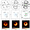 |
Fig. 1. (u,v) coverage of the EHT and representative ring image obtained by DoG-HIT (EHTC 2025) in 2017, 2018, and 2021. Upper panels: (u,v) with the SMT-KP (red) and PV-NOEMA baselines (green) highlighted. These are used to constrain the jet base emission. Middle panels: a zoomed-in view of the (u,v) coverage, highlighting the short and intermediate baselines. We also highlight the (u,v) coordinates related to spatial scales of 1000 μas and 200 μas, corresponding to the expected range for extended emission. Bottom panels: DoG-HIT image of the central ring obtained from these data (EHTC 2025). |
In EHTC (2025), the data were analyzed by seven teams using different imaging algorithms. The robustness of the reconstruction was demonstrated via cross-validation. Two teams used Difmap (Shepherd 1997), in combination with the AIPS task LPCAL (Leppanen et al. 1995) and GPCAL (Park et al. 2021, 2023a,b). The other teams used the RML methods DoG-HIT (Müller & Lobanov 2022, 2023a,b), ehtim (Chael et al. 2016, 2018), and MOEA/D (Müller et al. 2023; Mus et al. 2024a,b), as well as the Bayesian imaging techniques THEMIS (Broderick et al. 2020a) and Comrade (Tiede 2022). Although these imaging algorithms rely on different assumptions, they converge on a consistent recovered image structure on event horizon scales (EHTC 2025). We show a representative image from this analysis obtained by DoG-HIT in the bottom panels of Figure 1. The 2021 observations of M87* are well represented by a ring structure with an asymmetry oriented to the southwest. Although the total-intensity images are very consistent across years and methods, there is some significant evolution of the polarized structure over the years (for more details, we refer the reader to EHTC 2025). In this work, we focused on total intensity and leave the discussion of polarization of extended components for future work.
3. Jet base emission
3.1. Bump and offset in closure phases
We show the (u,v) coverage of the EHT in 2017, 2018, and 2021 in Figure 1 and highlight two new baselines introduced in 2021. The PV-NOEMA baseline is ∼1100 km in length, corresponding to on-sky spatial scales ∼250 μas; the SMT-KP baseline is ∼100 km in length, corresponding to ∼2500 μas scales. These intermediate baselines are sensitive to jet base emission, if it exists and is bright and compact enough to be detectable. However, each of these spatial scales is probed by a single baseline with a limited track length. Because of that, self-calibration techniques may inadvertently introduce or suppress extended emission if calibrated against a ring-only image or central point sources (e.g., Carilli & Thyagarajan 2022). To overcome this problem, we analyze data that were not self-calibrated, and use closure phases that are insensitive to station-based gain errors (e.g., Blackburn et al. 2020) to probe the jet base emission at scales accessible with SMT-KP and PV-NOEMA.
Three stations are required to construct closure phases. Because no other intermediate-length baselines are available, the closure triangles formed necessarily also probe small-scale structures. However, we can choose triangles that are particularly useful, i.e., show low variations during the track (indicating that the long baseline contribution is small or canceled), are long in duration, and have high signal-to-noise ratio (S/N). The high-sensitivity station ALMA satisfies all these requirements for both baselines of interest. We thus focused on the ALMA-SMT-KP and ALMA-PV-NOEMA triangles in this analysis.
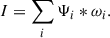
Since the small-scale information of the long ALMA baselines in those triangles cannot be disentangled from the intermediate-scale information, the jet base information has to be derived from the difference between the data and the ring-only image. In Figure 2 we show the closure phases on various triangles. The top panel displays an example triangle containing the ALMA-APEX baseline across the three years. The middle and bottom panels display the triangles of interest obtained for the small-scale ring images for different methods–one representative image is chosen for each framework–Difmap (CLEAN), DoG-HIT (RML) and Comrade (Bayesian). None of the imaging methods (marked by solid lines) can fully recover the closure phases with the compact ring image alone on these triangles. However, we note that the different imaging algorithms applied and validated various strategies to mitigate the effect of jet base emission on the ring images. These include the addition of large-scale Gaussian components that are not used to create the fits in Figure 2. Figure 2 displays the image fits without these additional factors, focusing solely on the compact ring feature.
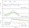 |
Fig. 2. ALMA-APEX-PV (top) closure phases of M87* as observed in 2017, 2018 and 2021. The ALMA-PV-NOEMA (middle) and ALMA-SMT-KP (bottom) closure phases on M87* observed on April 18, 2021 (figure is adapted from EHTC 2025) are shown together with ring-image models obtained with different imaging algorithms (see text for details). The top panel shows an example of a trivial closure phase triangle, where two stations are co-located, see Georgiev et al. (2025) for details. The image models are discrepant with the observed data by a few degrees, which may be attributable to intermediate-scale emission observed on the PV-NOEMA and SMT-KP baselines. |
In particular, the ALMA-PV-NOEMA triangle features a ‘bump’ that is not well captured by the ring images, and, similarly, ALMA-SMT-KP has a visible ‘offset’. Due to the high sensitivity on those triangles, the difference is significant despite its small magnitude.
One plausible explanation for this residual of a few degrees in the closure phase is a faint but measurable emission on intermediate spatial scales sensed by PV-NOEMA and SMT-KP.
3.2. Model
In the following, we motivate a simple model to explain the observed closure phase residuals on the two selected triangles. The triangle that includes the longer baseline PV-NOEMA features a bump with a period of a few hours. Conversely, the ALMA-SMT-KP triangle does not have a beating but a simple offset from the ring-image models. This suggests that the relevant spatial scales may be on the order of, or slightly larger than, the PV-NOEMA scale, as any larger structure would introduce a beating on the ALMA-SMT-KP triangle as well. Moreover, it needs to be located close to the image center. Such a closure phase signature is characteristic of a “binary model”; in our case it consists of the ring, which is not resolved by either of the two baselines, and an extra component.
Based on these simple considerations, we propose the following source model: the compact ring emission as seen on long baselines, with an additional, faint, Gaussian component located at scales 100 − 2000 μas from the center of the ring emission. This model gives four additional degrees of freedom, the x and y positions, the brightness F0, and the full width at half maximum (fwhm) of the Gaussian component. The model is selected to be as simple as possible to restrict the number of degrees of freedom, which is a necessary assumption for the model fitting due to the limited information on jet base emission present in the data. Because the PV-NOEMA and SMT-KP baselines are sensitive to two different spatial scales, they are not necessarily described by the same model component. Thus the model’s complexity can be trivially extended by allowing for an elliptical Gaussian component or even a second Gaussian component.
Deriving from these simple initial considerations, we can set approximate limits for the expected parameters of the additional Gaussian component. The size should be such that it is probed by the PV-NOEMA and SMT-KP baselines, creating a beating on the former within just two hours. Hence, it does not describe extended emission but most likely jet base emission with spatial scales similar to the ring diameter.
We refer to detailed analysis of the total flux density of the ring feature in EHT observations presented in EHTC (2024b). Although for the arcsecond scale structure in M87* typically flux densities between 1.0 Jy and 2.0 Jy were measured (Bower et al. 2015; Wielgus et al. 2020), for the milliarcsecond and microarcesond structure usually flux densities between 0.5 and 1.0 Jy have been reported (Doeleman et al. 2012; Akiyama et al. 2015; Kim et al. 2018; Wielgus et al. 2020; Lu et al. 2023), consistent with the values found by the EHT (EHTC 2019d, 2024b, 2025). The discrepancy between the ring image and the flux density detected with ALMA alone of about 1 Jy is due to the existence of an (as of yet) undetectable large-scale jet. The additional Gaussian component fitted in this manuscript is likely to explain some, but not necessarily all, of the missing flux. This sets an approximate upper limit of 0.5 Jy for the flux of the Gaussian component, preferably less.
4. Localization of the emission region
4.1. Impact of the model parameters
In the following analysis, we examine the impact of jet base emission when modeled as a Gaussian component. We base our analysis on a DoG-HIT reconstruction: since the algorithm separates small and large scale emission naturally, it is optimized to fit to the closure phases and closure amplitudes in the 2021 data. However, we note that the black hole shadow images obtained by various algorithms have similar characteristics on the ALMA-PV-NOEMA and ALMA-SMT-KP triangles with respect to the bump and the offset, see Figure 2.
Figure 3 shows the ring image obtained by DoG-HIT with an additional Gaussian added on top, varying some of the parameters described in Section 3.2. The upper part of the panels display the recovered central region with an additional Gaussian component in logarithmic scale. Panels e, f, h, and i show the observed closure phases (black markers) and model closure phases (solid lines) on the ALMA-PV-NOEMA triangle (AA-PV-NN) and ALMA-SMT-KP triangle (AA-MG-KP).
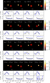 |
Fig. 3. Symmetric Gaussian component with varying parameters over the reconstructed DoG-HIT image as represented in Figure 1 represented in log scale. Different rows correspond to changes in the values of different parameters (see text for details). The solid lines represents the corresponding complete model (ring + Gaussian) closure phases on the respective triangles. |
The addition of a Gaussian component creates a periodic modulation – a beating – on the PV-NOEMA baseline. There are locations (primarily to the east and west of the ring, see Figure 3) where the beating is broadly aligned with the data, and locations where it misaligns and worsens the fit to the closure phase (primarily to the north). On the ALMA-SMT-KP triangle, the component produces a closure phase offset, which matches the data for some locations (good fits primarily to the West). The brightness of the component scales the amplitude of the beating and offset on the respective triangles. An overly bright Gaussian component overestimates the beating and the correction of the offset, while a too dim component underestimates the necessary corrections (first row of Figure 3). Finally, an overly compact component causes large-magnitude swings in the closure phase, while for a larger feature it is too smooth (fourth row in Figure 3).
These findings are summarized in Figure 4. In the left panel we show an example of reduced χ2 (χν2) of the ALMA-PV-NOEMA triangle as a function of the location of the Gaussian component with a fixed flux density of 60 mJy and a size of 180 μas. Locations 200 μas to the west or the east of the ring are preferred. Similarly, the middle panel shows the χν2 for the ALMA-SMT-KP triangle, with the preferred location to the southwest. In the right panel we show the combined χν2 and a preferred region to the southwest, roughly 300 μas to the West and 100 μas to the South of the ring. However, the presence of multiple regions with low χν2 indicates that the current model remains weakly constrained and degenerate.
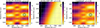 |
Fig. 4. χν2 achieved with the Gaussian model for a fixed width and brightness ratio, but varying position. The left and middle panels show the χν2 for the ALMA-PV-NOEMA and the ALMA-SMT-KP triangles, respectively, and the right panel shows the combined χν2. The contours indicate the position of the best-fit model. |
4.2. Symmetric Gaussian component
To obtain the maximum posterior position for a Gaussian component, we use the Markov chain Monte Carlo (MCMC) sampler EMCEE (Foreman-Mackey et al. 2013). We adopt uniform priors for the flux (F0 ∈ [0, 0.2] Jy), the location (x, y ∈ [ − 500, 500] μas), and the width (fwhms ∈ [50, 250] μas). The maximum posterior parameters are given in Table 1. The corner plots are shown in Appendix A (Figure A.1). The best fit component has a flux density of ∼60 mJy and is located towards the Southwestern portion of the ring.
We show the obtained ring image as well as the ring image with an additional Gaussian component in Figure 5. The respective fits of the Gaussian components to the ALMA-PV-NOEMA and ALMA-SMT-KP closure phases are shown in the panels e, f, h, and i. We highlighted notable improvements in the fitting quality of the closure phases visible from panel h and i. Despite the simplicity of the model, the χν2 is 1.29 for the bump (compared to 2.73 without the jet base emission), and 1.12 for the offset (compared to 2.52). The component has almost negligible impact on all other triangles; the χν2 over all triangles improves from 1.5 to 1.39. The χν2 does not increase for any triangle, see Appendix B for further details. In Figure B.2, we show the impact of the additional Gaussian component on the amplitudes for different baselines. Amplitudes on baselines longer than ∼2 Gλ stay mostly unaffected by the additional Gaussian component. This is reflected by the fit to the self-calibrated amplitudes shown in panel g and j in Figure 5 and the left panel in Figure B.2. The effect of the Gaussian component can be completely absorbed into the amplitude self-calibration.
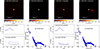 |
Fig. 5. Ring-only DoG-HIT image (panel a: linear scale, panel b: logarithmic scale) compared to the DoG-HIT ring image with an additional Gaussian (panel c and d). In the bottom row, we show the fit to the bump and offset in closure phases and the fit to the amplitudes for DoG-HIT (panels e,f,g) and for DoG-HIT with the symmetric Gaussian component added (panels h,i,j). |
Finally, synthetic data tests were performed in EHTC (2025). These tests also include the validation of a ring image with an extended jet component. The results of this test for all seven imaging techniques are described in Appendix D3 of that paper. We reprint the main result of this validation in Appendix B, Figure B.1. We note that all techniques were able to recover the ring emission correctly with exceptionally high cross-correlation > 0.995 for the total-intensity 2021 data.
We conclude that the addition of the Gaussian model does not worsen the otherwise excellent fit to the data obtained in EHTC (2025) with the black hole shadow images only. Vice versa, the Gaussian component only leaves a significant effect on the ALMA-PV-NOEMA and ALMA-SMT-KP triangles, exhibiting a small effect on the overall fitting statistics. Hence, based on the success of the fitting in the aforementioned study, and the synthetic data tests that were performed in EHTC (2025), we have no reason to question the validity of the ring emission presented in EHTC (2025).
4.3. Asymmetric Gaussian component
To explore the possibility of asymmetry of the jet base emission we extend the model by two additional parameters: the ratio of fwhmmaj and fwhmmin (ℛ) and the rotation angle of the asymmetric Gaussian component Φ, see Appendix C for additional details. We again use uniform priors (ℛ ∈ [0, 1], and Φ ∈ [ − 180 ° ,180 ° ]). Neither the flux density nor the position change significantly; however, the model prefers to be symmetric, and hence the rotation angle is poorly constrained. The χν2 values are 1.28 for the bump and 1.10 for the offset, i.e., there is no significant improvement to the fit. The best-fit values are provided in Table 1, we show the best-fit model in the left panel of Figure 6.
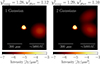 |
Fig. 6. Images for the best fits with an asymmetric Gaussian component (left) and two Gaussian components (right) in log scale. |
4.4. Two Gaussians
For completeness, we explore the possibility of a secondary Gaussian component in the fit. However, given the complexity of the model and limitations of the data, we constrain the second component in the positive y direction, that is, we allow the y position to vary only within [0, 500 μas]. In this way, we test the presence of the second component in the northern region, but allow all parameters to vary (12 parameters). The flux density of the first southern Gaussian is  . The second Gaussian has a flux density of
  . The first component is smaller in size compared to the previous modeling, but the positions do not vary significantly. The second, northern, component is relatively fainter. Since, the rotation angle for this component is poorly constrained, it prefers to be symmetric as well. The χν2 values are 1.29 for the bump and 1.10 for the offset. Thus, there is no statistical evidence for the inclusion of a secondary Gaussian component.
The Gaussian fit parameters are provided in Table 1, and the corner plot is provided in Appendix A. The third image in Figure 6 (right panel) represents the best-fit model consisting of two Gaussian components.
5. Alternative fitting scenarios
Due to the limited number of data points on the two chosen closure triangles, multiple plausible emission features may exist. In the previous section, we demonstrated that adding a simple Gaussian component to the compact emission provides a good fit to the data; the emission is most likely located southwest of the ring emission.
In this section, we discuss alternative models that may fit the data and discuss their validity. This list is not complete and focuses on some physically-motivated emission structures instead. Hence, we cannot rule out that alternative emission scenarios exist.
5.1. GMVA jet structure
At 86 GHz, Lu et al. (2023) imaged a ring-like feature together with the innermost jet in M87* with the GMVA complemented by the ALMA and the Greenland Telescope (GLT). Here, we discuss whether this jet structure would be able to fit the respective triangles. To this end, we need to extract the jet component of the GMVA image from the ring feature observed at 86 GHz, and stack this jet feature to the ring feature observed at 230 GHz.
Specifically, Kim et al. (2025) presented a reanalysis of this data set, among others, with DoG-HIT. In DoG-HIT, the image structure is represented in multiple spatial scales by wavelets Ψi:
 (1)
(1)
The smallest-scale wavelets describe the ring (the small-scale feature), and the largest spatial scales describe the jet emission. In this way, the image is naturally decomposed into the compact ring structure and the jet base emission across different spatial scales. We use this natural decomposition to study whether the jet observed by the GMVA provides a good fit: we filter out the ‘ring-components’ in the 86 GHz image by setting all small-scale wavelets to zero, then we add the 230 GHz EHT ring image and the jet emission at 86 GHz seen by the GMVA. Motivated by the findings in Section 4.1, the GMVA jet image is rescaled to add a flux density between 0.0 Jy and 0.2 Jy to match the 230 GHz ring image. We grid-search for the best flux density in this interval and find the best χ2 at an additional flux density of 0.06 Jy, consistent with the findings in Section 4.2. The results are shown in Figure 7. We note that we can absorb the large-scale jet component completely in the amplitude gains, providing a good fit to the self-calibrated amplitudes in both cases. The fit to the offset and the bump is improved by including the jet component. However, our model of the 86 GHz jet is not able to provide a good fit, performing worse than the simpler fiducial model presented in Section 4.2. This is likely a limitation of our attempt to scale the 86 GHz image, rather than an indication that the 86 GHz and 230 GHz emission structures are inherently different.
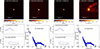 |
Fig. 7. Ring-only DoG-HIT image (first panel, top row: linear scale, second-panel first row: logarithmic scale) compared to the DoG-HIT ring image stacked with the jet observed with the GMVA (third and fourth panel, top row). In the bottom row, we show the fit to the bump and offset in closure phases and the fit to the amplitudes for DoG-HIT (left panels) and for DoG-HIT with the GMVA jet added (right panels). |
5.2. Imaging with weakened assumption on compactness
Next, we check whether we can find an alternative way of fitting the data, including the offset and the bump utilizing the DoG-HIT imaging algorithm. DoG-HIT represents the recovered image by a dictionary of wavelet functions Ψi and images at spatial sub-bands as described by Eq. 1. DoG-HIT utilizes a sparsity-constraining approach, effectively defining multiresolution support, i.e., a set of statistically-significant wavelet coefficients to describe the image. As demonstrated in Müller & Lobanov (2023a), the multiresolution support encodes two constraints: the location of the emission and the spatial scales needed to explain the emission at these locations. The latter relates to the (u,v) coverage, i.e., which spatial scales are measured.
This way, DoG-HIT allows for three alternative approaches to fit the bump and the offset. In the first approach, we investigate whether large spatial scales can account for the observed deviations without a constraint on the emission location or its spatial scale. In the second approach, we focus on localized emission in the ring. In the third approach, we constrain the location and spatial scales. For each approach, we take the ring-only image from DoG-HIT and try to improve the fit quality to the closure phases only, using a gradient descent approach with a small step size.
5.2.1. Fit without spatial scale and localization constraints
First, we do this fit without any mask on the spatial scales or the location of the emission, allowing every pixel to vary (labeled unmasked Figure 8, right column). The unmasked image fits the bump and also shows a much-improved fit to the offset. Moreover, improving the fits in the direction of the closure phases does not violate the match to the amplitudes. The recovered ring image shows no significant variation. However, comparing the unmasked image with the original image, which was masked in spatial scale and localization (Figure 8, left column), on a logarithmic scale, we observe that the improved precision has been achieved by fitting a ‘waffle-like pattern’ associated with the PV-NOEMA and SMT-KP baselines, which is nonphysical.
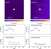 |
Fig. 8. Reconstruction of the ring and potential jet base emission, when restricted to spatial scales determined by DoG-HIT in the compact emission region (left panels, called masked), and completely unmasked (right panels, called unmasked). |
5.2.2. Fit with localization constraint
Here, we add a constraint on the emission location by performing the same gradient descent fit to the closure phases but only allowing the pixels on the ring to vary, defined by the 1% intensity contour in the DoG-HIT imagesy. The resulting reconstructions and model closure phases are shown in Figure 9.
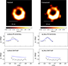 |
Fig. 9. Reconstruction of the ring and potential jet base emission when restricted to spatial scales determined by DoG-HIT in the compact emission region (left panels, called masked), and when restricted to the ring emission, but flexible in spatial scale (right panels, called unmasked). |
In this case, we can fit the bump reasonably well but have issues fitting the offset. A closer inspection of the structures that fit the bump in the top right panel of Figure 9 indicates that this fitting is achieved by asymmetries in the ring itself through a number of components. Each component exhibits structure significantly smaller than the resolution limit of roughly 20 μas.
5.2.3. Fit with localization and spatial constraints
Finally, we constrain the emission both by its localization and its spatial scale, as imprinted in the wavelet approach of DoG-HIT. The respective fitting quality is shown in the left columns of Figure 8 and Figure 9. Even if we fit for the ALMA-PV-NOEMA and ALMA-KP-SMT closure phases alone with a gradient-descent approach, restricted by the localization and spatial constraints imprinted by the wavelet dictionary, we remain limited in our potential to fit the bump or the offset.
This suggests that the model mismatch results from limiting the imaging to ring-scale emission only. This further supports the view that the bump and the offset are signatures of jet base emission, rather than artifacts from the imaging procedure being imprecise in its representation of the ring.
5.2.4. Data corruptions and systematic errors
Both the bump and offset are formally significant relative to a 0° closure phase, assuming the thermal errorbars are reliable. However, it is likely that the thermal errorbars underestimate the true error, as they do not account for non-closing errors such as polarization leakage (e.g., Broderick & Pesce 2020). Therefore, imaging methods add a fractional systematic Gaussian uncertainty to the errors of ∼2% of the visibility amplitudes (EHTC 2019c). In Appendix D we demonstrate that leakage cannot account for the bump or the offset. Nevertheless, we cannot rule out the possibility that other unknown sources of systematic error may corrupt the data.
5.3. Impact on previous EHT observations
The information about jet base emission has been derived primarily from the KP-SMT and PV-NOEMA baselines in this manuscript. These baselines are unique to the 2021 EHT data, as this was the first year in which the Kitt Peak telescope and NOEMA participated in EHT observations (EHTC 2025). In 2017 and 2018, LMT formed a baseline with the SMT of ∼1.3 Gλ (compared to 0.8 Gλ for PV-NOEMA in 2021), making it the shortest baseline between two stations that are not co-located (ALMA/APEX and SMA/JCMT) during these years. However, LMT did not participate in the 2021 observations. Here, we examine whether the jet base component derived in this manuscript – based on the enhanced coverage of the EHT in 2021 – would have a significant impact on data taken in 2017 and 2018. In other words, does our knowledge of an extended component influence the black hole shadow reconstructions presented in EHTC (2019a, 2024b, 2025)?
In Figure 10, we show the closure phases observed in 2017 (left panel) and 2018 (right panel) with the LMT-SMT baseline (black data points), and their respective fit to the DoG-HIT model of that year presented in EHTC (2025) (red line). The closure phases undergo a swing of almost 80° over the full duration of the observing track. This swing is completely explained by the ring models recovered by DoG-HIT. There is no additional feature visible that would motivate the fitting of an additional component in these years from the LMT-SMT baseline. In addition, we show with a blue dotted line the closure phases of the DoG-HIT model with the additional Gaussian component obtained from our analysis in 2021. In the bottom panels, we show the difference between the predicted closure phases with and without the additional Gaussian component compared to the noise level. The difference in closure phase introduced by our model on the LMT-SMT baseline is negligible. We conclude that, due to the lack of short baselines, the data obtained in 2017 and 2018 by the EHT are fully fitted by ring-only emission. Additionally, the Gaussian component identified in this work is not detectable on any baseline in the EHT longer than the PV-NOEMA baseline, and thus was not detectable/had no measurable impact on observations conducted in 2017 and 2018. Moreover, the component fitted here is relatively faint, only 60 mJy. Any significantly brighter component would introduce effects in ALMA-PV-NOEMA and ALMA-KP-SMT triangles larger than a few degrees, setting a robust upper limit for the amount of resolved jet emission in EHT observations to date.
 |
Fig. 10. Closure triangle formed by Chilean stations (ALMA/APEX), LMT, and SMT in 2017 (left panel) and 2018 (right panel). The LMT-SMT baseline is the shortest baseline between non-co-located stations in EHT observations of 2017 and 2018. Black markers: observed closure phases. Red line: fit to the DoG-HIT reconstruction in 2017 (left panel) and 2018 (right panel). Dark blue line: fit to the DoG-HIT reconstruction (ring) with an additional Gaussian model component determined from 2021 data as it would appear in 2017 (left panel) and 2018 (right panel). The line has been offset by a time offset of 0.1 hours to make it visible. In the bottom panels, we show the significance of the difference between the DoG-HIT model and the DoG-HIT model with additional Gaussian component, measured by the difference in ΨC divided by the closure phase error. In both years, the effect of the additional Gaussian component on the Chile-LMT-SMT closure phases is an order of magnitude smaller than the respective noise. |
6. Discussion
Broderick et al. (2022) found a component roughly 50 μas to the south and 50 μas to the West of the black hole shadow by modeling a narrow ring component to describe the black hole ring feature in the 2017 EHT observations (EHTC 2019a). This result is consistent with similar findings reported in Arras et al. (2022), Carilli & Thyagarajan (2022), although a robust detection could not be claimed by either study due to the lack of short and intermediate baselines in the 2017 EHT observations.
Broderick et al. (2022) demonstrated that the feature aligns well with the southern arm of the edge brightened jet observed at 86 GHz (Kim et al. 2018) when taking into account the expected core shift between 230 and 86 GHz. Recently Lu et al. (2023) observed the innermost jet in M87* at 86 GHz with the GMVA expanded by ALMA. They found a ring-like feature with an edge-brightened jet base. In Figure 11 we present the EHT results (green-colored contours) on top of the GMVA image (in virdis colormap). To this end, we use the intensity map reported by Kim et al. 2025 (a reanalysis of results reported in Lu et al. 2023) due to its improved resolution. The images are stacked by aligning the ring features observed at 230 and 86 GHz. By visual inspection, the jet base Gaussian component studied here aligns to first order with the southern arm of the edge-brightened jet observed with the GMVA. The second Gaussian component in the two-Gaussian model would align with the northern arm, but most likely represents a degeneracy in the posterior.
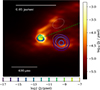 |
Fig. 11. Fiducial ring structure of the M87* black hole shadow (green contour) with a single Gaussian component (solid blue contours) corresponding to the best-fit parameters found in Section 4.2 (Table 1, first set) and double Gaussian components (dashed contours) corresponding to the best-fit parameters found in Section 4.4 (Table 1, second set), overplotted on the jet in M87* observed at 86 GHz (heatmap) with the GMVA (Lu et al. 2023; Kim et al. 2025). The green dotted line shows the jet orientation. |
The jet collimation profile at sub-milliarcsecond scales is parabolic. Kim et al. (2018) found a jet width profile W ∝ z0.5 (where z is the projected distance from the core), also in agreement with observations at milliarcsecond scales (Hada et al. 2013, 2016; Hada 2017). This parabolic shape is consistent with a jet driven either by black hole spin via the Blandford-Znajek mechanism (Blandford & Znajek 1977; Nakamura et al. 2018) or by the differential rotation of the accretion flow via the Blandford-Payne mechanism (Blandford & Payne 1982). The preference for a southwestern component in our model over a northwestern component is consistent with a rapidly rotating jet structure near the black hole (Broderick et al. 2022), however the scope for interpretation remains limited due to the limited amount of information. Lu et al. (2023) reported a deviation from the parabolic shape near the core (≤0.2 mas). This profile flattening may be a powerful indicator of the jet launching mechanism, potentially requiring an additional emission component, for example by non-thermal electrons in gravitationally unbound, non-relativistic winds (Nakamura et al. 2018; Park et al. 2019; Lu et al. 2023). While this is an anticipated observable for the EHT and its successors to connect the jet dynamics to the black hole and study jet launching mechanisms (EHTC 2024a), we note that the jet base component found in this study is too far out to make reliable conclusions about the physics of the jet within the first ten Schwarzschild radii.
7. Conclusions
We used the improved intermediate baseline coverage of the 2021 EHT campaign to search for resolved jet base emission around M87*. We found evidence for a faint offset component on angular scales accessible to the PV-NOEMA and KP-SMT baselines. Fitting a simple geometric model – a single offset Gaussian – yields a flux density of ∼60 mJy at a location ≈(−60, −320) μas relative to the ring center. The Gaussian component has fwhm ≈ 180 μ as.
Introducing the Gaussian component into the source model reduces the closure phase residuals on the ALMA-PV-NOEMA and ALMA-KP-SMT triangles. For the ALMA-PV-NOEMA triangle the χν2 falls from 2.73 to 1.29, and for the ALMA-KP-SMT triangle from 2.52 to 1.12; the χν2 for all triangles improves from 1.50 to 1.39; and it is improved on every single triangle, albeit the improvement is insignificant for most. This demonstrates that a compact, faint asymmetry at intermediate scales is an economical explanation for the observed closure phase structure in the 2021 data.
The recovered component’s position and scale are consistent with the southern/southwestern arm of the edge-brightened jet seen in the 86 GHz GMVA image. Stacking the component over the GMVA jet indicates a preference for an additional flux density of ∼60 mJy to match the EHT closure phases. However, the data do not statistically favor more complex models (an elliptical Gaussian component or a two-component component model) over the single Gaussian model.
We emphasize two important caveats. First, while our modeling improves the data-minus-model residuals, the limited number of intermediate baselines and the single-baseline sensitivity at the relevant spatial frequencies restrict a robust morphological reconstruction: other mathematically viable structures, including imaging artifacts consistent with the measured (u,v) sampling, cannot be fully excluded. Second, single-baseline or small-triangle measurements are susceptible to non-closing systematics. While we rule out polarization leakage as the origin of the signal and have performed imaging and synthetic data checks, unknown systematic errors cannot be completely ruled out. For these reasons, we conservatively treat the recovered Gaussian flux density as an upper limit on resolved jet base emission at spatial scales probed by the PV–NOEMA and KP–SMT baselines.
Finally, the presence of this faint component does not conflict with earlier EHT reconstructions from 2017, 2018, and 2021. The arrays in earlier years lacked the intermediate baselines required to detect emission at the spatial scales we probe here, so ring-only models adequately describe the earlier epochs. Excellent fitting quality, synthetic data tests, and the negligible effect of the Gaussian model on baselines longer than PV-NOEMA also indicate the robustness of the ring-only images obtained in 2021. The detection (or upper limit) reported here therefore complements earlier results and constrains where the EHT missing flux cannot reside: resolved, brighter emission ∼100 − 300 μas southeast and northeast relative to the ring is firmly ruled out by these closure triangles.
In summary, the 2021 EHT data provide the first constraints at 230 GHz on faint, asymmetric emission at intermediate scales near M87*, locating a plausible component southwest of the ring with a flux density < 0.1 Jy. Although this result is robust under the assumptions and tests performed, definitive confirmation and more precise constraints will require future EHT observations with higher sensitivity and improved intermediate-baseline coverage via additional stations and expanded frequency range.
References
- Abramowski, A., Acero, F., Aharonian, F., et al. 2012, ApJ, 746, 151 [NASA ADS] [CrossRef] [Google Scholar]
- Akiyama, K., Lu, R.-S., Fish, V. L., et al. 2015, ApJ, 807, 150 [NASA ADS] [CrossRef] [Google Scholar]
- Arras, P., Frank, P., Haim, P., et al. 2022, Nat. Astron., 6, 259 [NASA ADS] [CrossRef] [Google Scholar]
- Asada, K., & Nakamura, M. 2012, ApJ, 745, L28 [NASA ADS] [CrossRef] [Google Scholar]
- Asada, K., Nakamura, M., & Pu, H.-Y. 2016, ApJ, 833, 56 [NASA ADS] [CrossRef] [Google Scholar]
- Blackburn, L., Pesce, D. W., Johnson, M. D., et al. 2020, ApJ, 894, 31 [Google Scholar]
- Blandford, R. D., & Payne, D. G. 1982, MNRAS, 199, 883 [CrossRef] [Google Scholar]
- Blandford, R. D., & Znajek, R. L. 1977, MNRAS, 179, 433 [NASA ADS] [CrossRef] [Google Scholar]
- Bower, G. C., Dexter, J., Markoff, S., et al. 2015, ApJ, 811, L6 [NASA ADS] [CrossRef] [Google Scholar]
- Broderick, A. E., & Pesce, D. W. 2020, ApJ, 904, 126 [NASA ADS] [CrossRef] [Google Scholar]
- Broderick, A. E., Pesce, D. W., Gold, R., et al. 2022, ApJ, 935, 61 [NASA ADS] [CrossRef] [Google Scholar]
- Broderick, A. E., Gold, R., Karami, M., et al. 2020a, ApJ, 897, 139 [Google Scholar]
- Broderick, A. E., Pesce, D. W., Tiede, P., Pu, H.-Y., & Gold, R. 2020b, ApJ, 898, 9 [Google Scholar]
- Carilli, C. L., & Thyagarajan, N. 2022, ApJ, 924, 125 [NASA ADS] [CrossRef] [Google Scholar]
- Chael, A. A., Johnson, M. D., Narayan, R., et al. 2016, ApJ, 829, 11 [Google Scholar]
- Chael, A. A., Johnson, M. D., Bouman, K. L., et al. 2018, ApJ, 857, 23 [Google Scholar]
- Cui, Y., Hada, K., Kawashima, T., et al. 2023, Nature, 621, 711 [NASA ADS] [CrossRef] [Google Scholar]
- Deller, A. T., Tingay, S. J., Bailes, M., & West, C. 2007, PASP, 119, 318 [Google Scholar]
- Deller, A. T., Brisken, W. F., Phillips, C. J., et al. 2011, PASP, 123, 275 [Google Scholar]
- Doeleman, S. S., Fish, V. L., Schenck, D. E., et al. 2012, Science, 338, 355 [NASA ADS] [CrossRef] [Google Scholar]
- EHTC (Akiyama, K., et al.) 2019a, ApJ, 875, L1 [Google Scholar]
- EHTC (Akiyama, K., et al.) 2019b, ApJ, 875, L2 [Google Scholar]
- EHTC (Akiyama, K., et al.) 2019c, ApJ, 875, L3 [Google Scholar]
- EHTC (Akiyama, K., et al.) 2019d, ApJ, 875, L4 [Google Scholar]
- EHTC (Akiyama, K., et al.) 2019e, ApJ, 875, L5 [Google Scholar]
- EHTC (Akiyama, K., et al.) 2019f, ApJ, 875, L6 [Google Scholar]
- EHTC (Akiyama, K., et al.) 2021a, ApJ, 910, L12 [Google Scholar]
- EHTC (Akiyama, K., et al.) 2021b, ApJ, 910, L13 [Google Scholar]
- EHTC (Akiyama, K., et al.) 2023, ApJ, 957, L20 [NASA ADS] [CrossRef] [Google Scholar]
- EHTC 2024a, arXiv e-prints [arXiv:2410.02986] [Google Scholar]
- EHTC (Akiyama, K., et al.) 2024b, A&A, 681, A79 [NASA ADS] [CrossRef] [EDP Sciences] [Google Scholar]
- EHTC (Akiyama, K., et al.) 2025, A&A, 704, A91 [Google Scholar]
- Foreman-Mackey, D., Hogg, D. W., Lang, D., & Goodman, J. 2013, PASP, 125, 306 [Google Scholar]
- Georgiev, B., Tiede, P., von Fellenberg, S. D., et al. 2025, The location of the missing intrasite flux in M87* [Google Scholar]
- Goddi, C., Martí-Vidal, I., Messias, H., et al. 2021, ApJ, 910, L14 [NASA ADS] [CrossRef] [Google Scholar]
- Hada, K. 2017, Galaxies, 5, 2 [Google Scholar]
- Hada, K., Asada, K., Nakamura, M., & Kino, M. 2024, A&A Rev., 32, 5 [Google Scholar]
- Hada, K., Kino, M., Doi, A., et al. 2016, ApJ, 817, 131 [Google Scholar]
- Hada, K., Kino, M., Doi, A., et al. 2013, ApJ, 775, 70 [Google Scholar]
- Janssen, M., Goddi, C., van Bemmel, I. M., et al. 2019, A&A, 626, A75 [NASA ADS] [CrossRef] [EDP Sciences] [Google Scholar]
- Janssen, M., Radcliffe, J. F., & Wagner, J. 2022, Universe, 8, 527 [NASA ADS] [CrossRef] [Google Scholar]
- Kim, J. Y., Krichbaum, T. P., Lu, R. S., et al. 2018, A&A, 616, A188 [NASA ADS] [CrossRef] [EDP Sciences] [Google Scholar]
- Kim, J.-Y., Savolainen, T., Voitsik, P., et al. 2023, ApJ, 952, 34 [NASA ADS] [CrossRef] [Google Scholar]
- Kim, J.-S., Müller, H., Nikonov, A. S., et al. 2025, A&A, 696, 11 [Google Scholar]
- Leppanen, K. J., Zensus, J. A., & Diamond, P. J. 1995, AJ, 110, 2479 [Google Scholar]
- Lister, M. L., Aller, M. F., Aller, H. D., et al. 2018, ApJS, 234, 12 [CrossRef] [Google Scholar]
- Lu, R.-S., Asada, K., Krichbaum, T. P., et al. 2023, Nature, 616, 686 [CrossRef] [Google Scholar]
- Marshall, H. L., Miller, B. P., Davis, D. S., et al. 2002, ApJ, 564, 683 [Google Scholar]
- Martí-Vidal, I., Roy, A., Conway, J., & Zensus, A. J. 2016, A&A, 587, A143 [NASA ADS] [CrossRef] [EDP Sciences] [Google Scholar]
- Müller, H. 2024, A&A, 689, A299 [NASA ADS] [CrossRef] [EDP Sciences] [Google Scholar]
- Müller, H., & Lobanov, A. P. 2022, A&A, 666, A137 [NASA ADS] [CrossRef] [EDP Sciences] [Google Scholar]
- Müller, H., & Lobanov, A. P. 2023a, A&A, 673, A151 [NASA ADS] [CrossRef] [EDP Sciences] [Google Scholar]
- Müller, H., & Lobanov, A. P. 2023b, A&A, 672, A26 [NASA ADS] [CrossRef] [EDP Sciences] [Google Scholar]
- Müller, H., Mus, A., & Lobanov, A. 2023, A&A, 675, A60 [NASA ADS] [CrossRef] [EDP Sciences] [Google Scholar]
- Mus, A., Müller, H., & Lobanov, A. 2024a, A&A, 688, A100 [NASA ADS] [CrossRef] [EDP Sciences] [Google Scholar]
- Mus, A., Müller, H., Martí-Vidal, I., & Lobanov, A. 2024b, A&A, 684, A55 [NASA ADS] [CrossRef] [EDP Sciences] [Google Scholar]
- Nakamura, M., & Asada, K. 2013, ApJ, 775, 118 [NASA ADS] [CrossRef] [Google Scholar]
- Nakamura, M., Asada, K., Hada, K., et al. 2018, ApJ, 868, 146 [Google Scholar]
- Nikonov, A. S., Kovalev, Y. Y., Kravchenko, E. V., Pashchenko, I. N., & Lobanov, A. P. 2023, MNRAS, 526, 5949 [NASA ADS] [CrossRef] [Google Scholar]
- Park, J., Asada, K., & Byun, D.-Y. 2023a, ApJ, 958, 27 [NASA ADS] [CrossRef] [Google Scholar]
- Park, J., Asada, K., & Byun, D.-Y. 2023b, ApJ, 958, 28 [NASA ADS] [CrossRef] [Google Scholar]
- Park, J., Hada, K., Kino, M., et al. 2019, ApJ, 871, 257 [Google Scholar]
- Park, J., Asada, K., Nakamura, M., et al. 2021, ApJ, 922, 180 [NASA ADS] [CrossRef] [Google Scholar]
- Perlman, E. S., Adams, S. C., Cara, M., et al. 2011, ApJ, 743, 119 [NASA ADS] [CrossRef] [Google Scholar]
- Pordes, R., Petravick, D., Kramer, B., et al. 2007, J. Phys. Conf. Ser., 78, 012057 [NASA ADS] [CrossRef] [Google Scholar]
- Röder, J., Wielgus, M., Jensen, J. B., Anand, G. S., & Tully, R. B. 2025, A&A, 701, L12 [NASA ADS] [CrossRef] [EDP Sciences] [Google Scholar]
- Sfiligoi, I., Bradley, D. C., Holzman, B., et al. 2009, in 2009 WRI World Congress on Computer Science and Information Engineering, 2, 428 [CrossRef] [Google Scholar]
- Shepherd, M. C. 1997, in Astronomical Data Analysis Software and Systems VI, eds. G. Hunt, & H. Payne, ASP Conf. Ser., 125, 77 [Google Scholar]
- Thompson, A. R., Moran, J. M., & Swenson, G. W., Jr 2017, Interferometry and Synthesis in Radio Astronomy, 3rd edn. (Springer) [Google Scholar]
- Tiede, P. 2022, J. Open Source Software, 7, 4457 [Google Scholar]
- von Fellenberg, S. D., García, R., Janssen, M., et al. 2025, Res. Notes Am. Astron. Soc., 9, 134 [Google Scholar]
- Walker, R. C., Hardee, P. E., Davies, F. B., Ly, C., & Junor, W. 2018, ApJ, 855, 128 [Google Scholar]
- Wielgus, M., Akiyama, K., Blackburn, L., et al. 2020, ApJ, 901, 67 [Google Scholar]
That is, images of a variety of simple geometric structures, physically motivated structures, as well as simulations of accretion flow (EHTC 2025).
Appendix A: Corner plots
In the following, we show the MCMC corner plots of the three model fits that we performed. Figure A.1 displays the corner plot of the four-parameter Gaussian model, Figure A.2 displays the corner plot of the six-parameter Gaussian model, and Figure A.3 displays the fit with a twelve-parameter double Gaussian model.
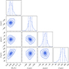 |
Fig. A.1. Corner plot showcasing our estimates for the location (x, y in units of μ as), flux (F0 in units of Jy), and width (σ in units of μ as) of the Gaussian toy model. |
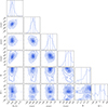 |
Fig. A.2. Same as Figure A.1 but with two additional parameters: ℛ, the ratio of fwhmmaj and fwhmmin, and Φ, the rotation angle, of the asymmetric Gaussian toy model. See Section 4.3 for more details. |
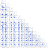 |
Fig. A.3. Same as Figure A.1 but for two asymmetric Gaussian toy models. See Section 4.4 for more details. |
Appendix B: Effect on visibility amplitude
In Figure B.1 we show the evaluation of the synthetic data test performed with an extended jet component in EHTC (2025). In Figure B.2 we show the amplitudes of the ring model, the fiducial model, and the difference between the two models as a function of the projected baseline length.
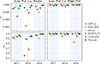 |
Fig. B.1. Figure D3 of EHTC (2025). Cross-correlation between the recovered ring model and synthetic ground truth model for seven different imaging techniques in 2017, 2018, and 2021. The synthetic data included a large-scale jet component. Upper panels show the cross-correlation in total intensity, lower panels in polarization. Despite the synthetic data containing a large scale jet component, the black hole shadow has been recovered for all methods and all years with exceptional accuracy, achieving cross-correlations > 0.995 in total intensity in 2021. |
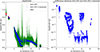 |
Fig. B.2. Left panel: comparison of the predicted amplitudes for the DoG-HIT ring-only image (red markers), the DoG-HIT image with additional Gaussian component (blue markers), and the self-calibrated visibility amplitudes (green markers) as a function of projected baseline length. Right panel: the difference between the predicted visibilities for the DoG-HIT model and DoG-HIT with the additional Gaussian component as a function of projected baseline length. The plot demonstrates that the additional Gaussian component has no sizeable effect on baselines longer than PV-NOEMA. |
Appendix C: Parameter exploration for 6 parameter Gaussian model
We demonstrate the effect of adding two additional degrees of freedom to the model with an asymmetric Gaussian component that can be rotated around its axis. In Figure B.3 we show that these parameters can be constrained in the extreme case of a very asymmetric Gaussian component. However, these parameters are poorly constrained.
Appendix D: Impact of non-closing errors
Because the phase signature of the offset Gaussian component(s) is small, we cannot completely rule out systematic effects as an origin. Here, we assess the impact of one known non-closing error: polarization leakage. Polarization leakage causes signal dispersion from one correlation of polarization handedness (e.g., RR) to another (e.g., LL), and is baseline-based in nature (e.g., Müller 2024). One data-driven test to rule out leakage as the cause of the bump and offset is to compare the phase-residuals of the RR − LL closure phases on the respective triangles (Figure ). Under the assumptions that there is no significant leakage and that circular polarization is → 0, the difference between the parallel hands closure phases is zero. While there is a small offset on the ALMA-PV-NOEMA triangle, neither the bump nor the offset can be explained by a difference between the parallel hands, and we thus conclude that the signal is not caused by polarization leakage. The difference in the ALMA-PV-NOEMA triangle may be caused by either intrinsic circular polarization of the source or by leakage, and we thus place a limit on this type of non-closing error of ∼1°.
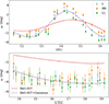 |
Fig. D.1. Comparison of the RR (orange) and LL (green) closure phases on the ALMA-NOEMA-PV (top) and ALMA-KP-SMT triangles (bottom). The red line indicates the DoG-HIT ring model, the magenta line indicates the DoG-HIT model with an additional Gaussian component. |
Appendix E: Acknowledgments
We thank the anonymous reviewer for their insightful comments and suggestions. Saurabh received financial support for this research from the International Max Planck Research School (IMPRS) for Astronomy and Astrophysics at the Universities of Bonn and Cologne. This work was supported by the M2FINDERS project funded by the European Research Council (ERC) under the European Union’s Horizon 2020 Research and Innovation Programme (Grant Agreement No. 101018682). SDvF gratefully acknowledges the support of the Alexander von Humboldt Foundation through a Feodor Lynen Fellowship and thanks CITA for their hospitality and collaboration. The Event Horizon Telescope Collaboration thanks the following organizations and programs: the Academia Sinica; the Research Council of Finland (project 362572); the Agencia Nacional de Investigación y Desarrollo (ANID), Chile via NCN19_058 (TITANs), Fondecyt 1221421 and BASAL FB210003; the Alexander von Humboldt Stiftung (including the Feodor Lynen Fellowship); an Alfred P. Sloan Research Fellowship; Allegro, the European ALMA Regional Centre node in the Netherlands, the NL astronomy research network NOVA and the astronomy institutes of the University of Amsterdam, Leiden University, and Radboud University; the ALMA North America Development Fund; the Astrophysics and High Energy Physics programme by MCIN (with funding from European Union NextGenerationEU, PRTR-C17I1); the Black Hole Initiative, which is funded by grants from the John Templeton Foundation (60477, 61497, 62286) and the Gordon and Betty Moore Foundation (Grant GBMF-8273) - although the opinions expressed in this work are those of the author and do not necessarily reflect the views of these Foundations; the Brinson Foundation; the Canada Research Chairs (CRC) program; Chandra DD7-18089X and TM6-17006X; the China Scholarship Council; the China Postdoctoral Science Foundation fellowships (2020M671266, 2022M712084); ANID through Fondecyt Postdoctorado (project 3250762); Conicyt through Fondecyt Postdoctorado (project 3220195); Consejo Nacional de Humanidades, Ciencia y Tecnología (CONAHCYT, Mexico, projects U0004-246083, U0004-259839, F0003-272050, M0037-279006, F0003-281692, 104497, 275201, 263356, CBF2023-2024-1102, 257435); the Colfuturo Scholarship; the Consejo Superior de Investigaciones Científicas (grant 2019AEP112); the Delaney Family via the Delaney Family John A. Wheeler Chair at Perimeter Institute; Dirección General de Asuntos del Personal Académico-Universidad Nacional Autónoma de México (DGAPA-UNAM, projects IN112820 and IN108324); the Dutch Research Council (NWO) for the VICI award (grant 639.043.513), the grant OCENW.KLEIN.113, and the Dutch Black Hole Consortium (with project No. NWA 1292.19.202) of the research programme the National Science Agenda; the Dutch National Supercomputers, Cartesius and Snellius (NWO grant 2021.013); the EACOA Fellowship awarded by the East Asia Core Observatories Association, which consists of the Academia Sinica Institute of Astronomy and Astrophysics, the National Astronomical Observatory of Japan, Center for Astronomical Mega-Science, Chinese Academy of Sciences, and the Korea Astronomy and Space Science Institute; the European Research Council (ERC) Synergy Grant “BlackHoleCam: Imaging the Event Horizon of Black Holes” (grant 610058) and Synergy Grant “BlackHolistic: Colour Movies of Black Holes: Understanding Black Hole Astrophysics from the Event Horizon to Galactic Scales” (grant 10107164); the European Union Horizon 2020 research and innovation programme under grant agreements RadioNet (No. 730562), M2FINDERS (No. 101018682); the European Research Council for advanced grant “JETSET: Launching, propagation and emission of relativistic jets from binary mergers and across mass scales” (grant No. 884631); the European Horizon Europe staff exchange (SE) programme HORIZON-MSCA-2021-SE-01 grant NewFunFiCO (No. 10108625); the Horizon ERC Grants 2021 programme under grant agreement No. 101040021; the FAPESP (Fundação de Amparo á Pesquisa do Estado de São Paulo) under grant 2021/01183-8; the Fondes de Recherche Nature et Technologies (FRQNT); the Fondo CAS-ANID folio CAS220010; the Generalitat Valenciana (grants APOSTD/2018/177 and ASFAE/2022/018) and GenT Program (project CIDEGENT/2018/021); the Gordon and Betty Moore Foundation (GBMF-3561, GBMF-5278, GBMF-10423); the Institute for Advanced Study; the ICSC – Centro Nazionale di Ricerca in High Performance Computing, Big Data and Quantum Computing, funded by European Union – NextGenerationEU; the Istituto Nazionale di Fisica Nucleare (INFN) sezione di Napoli, iniziative specifiche TEONGRAV; the International Max Planck Research School for Astronomy and Astrophysics at the Universities of Bonn and Cologne; the Italian Ministry of University and Research (MUR)– Project CUP F53D23001260001, funded by the European Union – NextGenerationEU; Deutsche Forschungsgemeinschaft (DFG) research grant “Jet physics on horizon scales and beyond” (grant No. 443220636) and DFG research grant 443220636; Joint Columbia/Flatiron Postdoctoral Fellowship (research at the Flatiron Institute is supported by the Simons Foundation); the Japan Ministry of Education, Culture, Sports, Science and Technology (MEXT; grant JPMXP1020200109); the Japan Society for the Promotion of Science (JSPS) Grant-in-Aid for JSPS Research Fellowship (JP17J08829); the Joint Institute for Computational Fundamental Science, Japan; the Key Research Program of Frontier Sciences, Chinese Academy of Sciences (CAS, grants QYZDJ-SSW-SLH057, QYZDJSSW-SYS008, ZDBS-LY-SLH011); the Leverhulme Trust Early Career Research Fellowship; the Max-Planck-Gesellschaft (MPG); the Max Planck Partner Group of the MPG and the CAS; the MEXT/JSPS KAKENHI (grants 18KK0090, JP21H01137, JP18H03721, JP18K13594, 18K03709, JP19K14761, 18H01245, 25120007, 19H01943, 21H01137, 21H04488, 22H00157, 23K03453); the MICINN Research Projects PID2019-108995GB-C22, PID2022-140888NB-C22; the MIT International Science and Technology Initiatives (MISTI) Funds; the Ministry of Science and Technology (MOST) of Taiwan (103-2119-M-001-010-MY2, 105-2112-M-001-025-MY3, 105-2119-M-001-042, 106-2112-M-001-011, 106-2119-M-001-013, 106-2119-M-001-027, 106-2923-M-001-005, 107-2119-M-001-017, 107-2119-M-001-020, 107-2119-M-001-041, 107-2119-M-110-005, 107-2923-M-001-009, 108-2112-M-001-048, 108-2112-M-001-051, 108-2923-M-001-002, 109-2112-M-001-025, 109-2124-M-001-005, 109-2923-M-001-001, 110-2112-M-001-033, 110-2124-M-001-007 and 110-2923-M-001-001); the National Science and Technology Council (NSTC) of Taiwan (111-2124-M-001-005, 112-2124-M-001-014, 112-2112-M-003-010-MY3, and 113-2124-M-001-008); the Ministry of Education (MoE) of Taiwan Yushan Young Scholar Program; the Physics Division, National Center for Theoretical Sciences of Taiwan; the National Aeronautics and Space Administration (NASA, Fermi Guest Investigator grant 80NSSC23K1508, NASA Astrophysics Theory Program grant 80NSSC20K0527, NASA NuSTAR award 80NSSC20K0645); NASA Hubble Fellowship Program Einstein Fellowship; NASA Hubble Fellowship grants HST-HF2-51431.001-A, HST-HF2-51482.001-A, HST-HF2-51539.001-A, HST-HF2-51552.001A awarded by the Space Telescope Science Institute, which is operated by the Association of Universities for Research in Astronomy, Inc., for NASA, under contract NAS5-26555; the National Institute of Natural Sciences (NINS) of Japan; the National Key Research and Development Program of China (grant 2016YFA0400704, 2017YFA0402703, 2016YFA0400702); the National Science and Technology Council (NSTC, grants NSTC 111-2112-M-001 -041, NSTC 111-2124-M-001-005, NSTC 112-2124-M-001-014); the US National Science Foundation (NSF, grants AST-0096454, AST-0352953, AST-0521233, AST-0705062, AST-0905844, AST-0922984, AST-1126433, OIA-1126433, AST-1140030, DGE-1144085, AST-1207704, AST-1207730, AST-1207752, MRI-1228509, OPP-1248097, AST-1310896, AST-1440254, AST-1555365, AST-1614868, AST-1615796, AST-1715061, AST-1716327, AST-1726637, OISE-1743747, AST-1743747, AST-1816420, AST-1935980, AST-1952099, AST-2034306, AST-2205908, AST-2307887, AST-2407810); NSF Astronomy and Astrophysics Postdoctoral Fellowship (AST-1903847); the Natural Science Foundation of China (grants 11650110427, 10625314, 11721303, 11725312, 11873028, 11933007, 11991052, 11991053, 12192220, 12192223, 12273022, 12325302, 12303021); the Natural Sciences and Engineering Research Council of Canada (NSERC); the National Research Foundation of Korea (the Global PhD Fellowship Grant: grants NRF-2015H1A2A1033752; the Korea Research Fellowship Program: NRF-2015H1D3A1066561; Brain Pool Program: RS-2024-00407499; Basic Research Support Grant 2019R1F1A1059721, 2021R1A6A3A01086420, 2022R1C1C1005255, RS-2022-NR071771, 2022R1F1A1075115); the POSCO Science Fellowship of the POSCO TJ Park Foundation; NOIRLab, which is managed by the Association of Universities for Research in Astronomy (AURA) under a cooperative agreement with the National Science Foundation; Onsala Space Observatory (OSO) national infrastructure, for the provisioning of its facilities/observational support (OSO receives funding through the Swedish Research Council under grant 2017-00648); the Perimeter Institute for Theoretical Physics (research at Perimeter Institute is supported by the Government of Canada through the Department of Innovation, Science and Economic Development and by the Province of Ontario through the Ministry of Research, Innovation and Science); the Portuguese Foundation for Science and Technology (FCT) grants (Individual CEEC program – 5th edition, CIDMA through the FCT Multi-Annual Financing Program for R&D Units UID/04106, CERN/FIS-PAR/0024/2021, 2022.04560.PTDC); the Princeton Gravity Initiative; the Spanish Ministerio de Ciencia, Innovación y Universidades (grants PID2022-140888NB-C21, PID2022-140888NB-C22, PID2023-147883NB-C21, RYC2023-042988-I); the Severo Ochoa grant CEX2021-001131-S funded by MICIU/AEI/10.13039/501100011033; The European Union’s Horizon Europe research and innovation program under grant agreement No. 101093934 (RADIOBLOCKS); The European Union “NextGenerationEU”, the Recovery, Transformation and Resilience Plan, the CUII of the Andalusian Regional Government and the Spanish CSIC through grant AST22_00001_Subproject_10; “la Caixa” Foundation (ID 100010434) through fellowship codes LCF/BQ/DI22/11940027 and LCF/BQ/DI22/11940030; the University of Pretoria for financial aid in the provision of the new Cluster Server nodes and SuperMicro (USA) for a SEEDING GRANT approved toward these nodes in 2020; the Shanghai Municipality orientation program of basic research for international scientists (grant no. 22JC1410600); the Shanghai Pilot Program for Basic Research, Chinese Academy of Science, Shanghai Branch (JCYJ-SHFY-2021-013); the Simons Foundation (grant 00001470); the Spanish Ministry for Science and Innovation grant CEX2021-001131-S funded by MCIN/AEI/10.13039/501100011033; the Spinoza Prize SPI 78-409; the South African Research Chairs Initiative, through the South African Radio Astronomy Observatory (SARAO, grant ID 77948), which is a facility of the National Research Foundation (NRF), an agency of the Department of Science and Innovation (DSI) of South Africa; the Swedish Research Council (VR); the Taplin Fellowship; the Toray Science Foundation; the UK Science and Technology Facilities Council (grant no. ST/X508329/1); the US Department of Energy (USDOE) through the Los Alamos National Laboratory (operated by Triad National Security, LLC, for the National Nuclear Security Administration of the USDOE, contract 89233218CNA000001); and the YCAA Prize Postdoctoral Fellowship. This work was also supported by the National Research Foundation of Korea (NRF) grant funded by the Korea government(MSIT) (RS-2024-00449206). We acknowledge support from the Coordenação de Aperfeiçoamento de Pessoal de Nível Superior (CAPES) of Brazil through PROEX grant number 88887.845378/2023-00. We acknowledge financial support from Millenium Nucleus NCN23_002 (TITANs) and Comité Mixto ESO-Chile.
We thank the staff at the participating observatories, correlation centers, and institutions for their enthusiastic support. This paper makes use of the following ALMA data: ADS/JAO.ALMA#2017.1.00841.V and ADS/JAO.ALMA#2019.1.01797.V. ALMA is a partnership of the European Southern Observatory (ESO; Europe, representing its member states), NSF, and National Institutes of Natural Sciences of Japan, together with National Research Council (Canada), Ministry of Science and Technology (MOST; Taiwan), Academia Sinica Institute of Astronomy and Astrophysics (ASIAA; Taiwan), and Korea Astronomy and Space Science Institute (KASI; Republic of Korea), in cooperation with the Republic of Chile. The Joint ALMA Observatory is operated by ESO, Associated Universities, Inc. (AUI)/NRAO, and the National Astronomical Observatory of Japan (NAOJ). The NRAO is a facility of the NSF operated under cooperative agreement by AUI. This research used resources of the Oak Ridge Leadership Computing Facility at the Oak Ridge National Laboratory, which is supported by the Office of Science of the U.S. Department of Energy under contract No. DE-AC05-00OR22725; the ASTROVIVES FEDER infrastructure, with project code IDIFEDER-2021-086; the computing cluster of Shanghai VLBI correlator supported by the Special Fund for Astronomy from the Ministry of Finance in China; We also thank the Center for Computational Astrophysics, National Astronomical Observatory of Japan. This work was supported by FAPESP (Fundacao de Amparo a Pesquisa do Estado de Sao Paulo) under grant 2021/01183-8.
APEX is a collaboration between the Max-Planck-Institut für Radioastronomie (Germany), ESO, and the Onsala Space Observatory (Sweden). The SMA is a joint project between the SAO and ASIAA and is funded by the Smithsonian Institution and the Academia Sinica. The JCMT is operated by the East Asian Observatory on behalf of the NAOJ, ASIAA, and KASI, as well as the Ministry of Finance of China, Chinese Academy of Sciences, and the National Key Research and Development Program (No. 2017YFA0402700) of China and Natural Science Foundation of China grant 11873028. Additional funding support for the JCMT is provided by the Science and Technologies Facility Council (UK) and participating universities in the UK and Canada. The LMT is a project operated by the Instituto Nacional de Astrófisica, Óptica, y Electrónica (Mexico) and the University of Massachusetts at Amherst (USA). The IRAM 30 m telescope on Pico Veleta, Spain and the NOEMA interferometer on Plateau de Bure, France are operated by IRAM and supported by CNRS (Centre National de la Recherche Scientifique, France), MPG (Max-Planck-Gesellschaft, Germany), and IGN (Instituto Geográfico Nacional, Spain). The SMT is operated by the Arizona Radio Observatory, a part of the Steward Observatory of the University of Arizona, with financial support of operations from the State of Arizona and financial support for instrumentation development from the NSF. Support for SPT participation in the EHT is provided by the National Science Foundation through award OPP-1852617 to the University of Chicago. Partial support is also provided by the Kavli Institute of Cosmological Physics at the University of Chicago. The SPT hydrogen maser was provided on loan from the GLT, courtesy of ASIAA.
This work used the Extreme Science and Engineering Discovery Environment (XSEDE), supported by NSF grant ACI-1548562, and CyVerse, supported by NSF grants DBI-0735191, DBI-1265383, and DBI-1743442. XSEDE Stampede2 resource at TACC was allocated through TG-AST170024 and TG-AST080026N. XSEDE JetStream resource at PTI and TACC was allocated through AST170028. This research is part of the Frontera computing project at the Texas Advanced Computing Center through the Frontera Large-Scale Community Partnerships allocation AST20023. Frontera is made possible by National Science Foundation award OAC-1818253. This research was done using services provided by the OSG Consortium (Pordes et al. 2007; Sfiligoi et al. 2009), which is supported by the National Science Foundation award Nos. 2030508 and 1836650. Additional work used ABACUS2.0, which is part of the eScience center at Southern Denmark University, and the Kultrun Astronomy Hybrid Cluster (projects Conicyt Programa de Astronomia Fondo Quimal QUIMAL170001, Conicyt PIA ACT172033, Fondecyt Iniciacion 11170268, Quimal 220002). Simulations were also performed on the SuperMUC cluster at the LRZ in Garching, on the LOEWE cluster in CSC in Frankfurt, on the HazelHen cluster at the HLRS in Stuttgart, and on the Pi2.0 and Siyuan Mark-I at Shanghai Jiao Tong University. The computer resources of the Finnish IT Center for Science (CSC) and the Finnish Computing Competence Infrastructure (FCCI) project are acknowledged. This research was enabled in part by support provided by Compute Ontario (http://computeontario.ca), Calcul Quebec (http://www.calculquebec.ca), and the Digital Research Alliance of Canada (https://alliancecan.ca/en).
The EHTC has received generous donations of FPGA chips from Xilinx Inc., under the Xilinx University Program. The EHTC has benefited from technology shared under open-source license by the Collaboration for Astronomy Signal Processing and Electronics Research (CASPER). The EHT project is grateful to T4Science and Microsemi for their assistance with hydrogen masers. This research has made use of NASA’s Astrophysics Data System. We gratefully acknowledge the support provided by the extended staff of the ALMA, from the inception of the ALMA Phasing Project through the observational campaigns of 2017 and 2018. We would like to thank A. Deller and W. Brisken for EHT-specific support with the use of DiFX. We thank Martin Shepherd for the addition of extra features in the Difmap software that were used for the CLEAN imaging results presented in this paper. We acknowledge the significance that Maunakea, where the SMA and JCMT EHT stations are located, has for the indigenous Hawaiian people.
All Tables
All Figures
|
Fig. 1. (u,v) coverage of the EHT and representative ring image obtained by DoG-HIT (EHTC 2025) in 2017, 2018, and 2021. Upper panels: (u,v) with the SMT-KP (red) and PV-NOEMA baselines (green) highlighted. These are used to constrain the jet base emission. Middle panels: a zoomed-in view of the (u,v) coverage, highlighting the short and intermediate baselines. We also highlight the (u,v) coordinates related to spatial scales of 1000 μas and 200 μas, corresponding to the expected range for extended emission. Bottom panels: DoG-HIT image of the central ring obtained from these data (EHTC 2025). |
| In the text | |
|
Fig. 2. ALMA-APEX-PV (top) closure phases of M87* as observed in 2017, 2018 and 2021. The ALMA-PV-NOEMA (middle) and ALMA-SMT-KP (bottom) closure phases on M87* observed on April 18, 2021 (figure is adapted from EHTC 2025) are shown together with ring-image models obtained with different imaging algorithms (see text for details). The top panel shows an example of a trivial closure phase triangle, where two stations are co-located, see Georgiev et al. (2025) for details. The image models are discrepant with the observed data by a few degrees, which may be attributable to intermediate-scale emission observed on the PV-NOEMA and SMT-KP baselines. |
| In the text | |
|
Fig. 3. Symmetric Gaussian component with varying parameters over the reconstructed DoG-HIT image as represented in Figure 1 represented in log scale. Different rows correspond to changes in the values of different parameters (see text for details). The solid lines represents the corresponding complete model (ring + Gaussian) closure phases on the respective triangles. |
| In the text | |
|
Fig. 4. χν2 achieved with the Gaussian model for a fixed width and brightness ratio, but varying position. The left and middle panels show the χν2 for the ALMA-PV-NOEMA and the ALMA-SMT-KP triangles, respectively, and the right panel shows the combined χν2. The contours indicate the position of the best-fit model. |
| In the text | |
|
Fig. 5. Ring-only DoG-HIT image (panel a: linear scale, panel b: logarithmic scale) compared to the DoG-HIT ring image with an additional Gaussian (panel c and d). In the bottom row, we show the fit to the bump and offset in closure phases and the fit to the amplitudes for DoG-HIT (panels e,f,g) and for DoG-HIT with the symmetric Gaussian component added (panels h,i,j). |
| In the text | |
|
Fig. 6. Images for the best fits with an asymmetric Gaussian component (left) and two Gaussian components (right) in log scale. |
| In the text | |
|
Fig. 7. Ring-only DoG-HIT image (first panel, top row: linear scale, second-panel first row: logarithmic scale) compared to the DoG-HIT ring image stacked with the jet observed with the GMVA (third and fourth panel, top row). In the bottom row, we show the fit to the bump and offset in closure phases and the fit to the amplitudes for DoG-HIT (left panels) and for DoG-HIT with the GMVA jet added (right panels). |
| In the text | |
|
Fig. 8. Reconstruction of the ring and potential jet base emission, when restricted to spatial scales determined by DoG-HIT in the compact emission region (left panels, called masked), and completely unmasked (right panels, called unmasked). |
| In the text | |
|
Fig. 9. Reconstruction of the ring and potential jet base emission when restricted to spatial scales determined by DoG-HIT in the compact emission region (left panels, called masked), and when restricted to the ring emission, but flexible in spatial scale (right panels, called unmasked). |
| In the text | |
|
Fig. 10. Closure triangle formed by Chilean stations (ALMA/APEX), LMT, and SMT in 2017 (left panel) and 2018 (right panel). The LMT-SMT baseline is the shortest baseline between non-co-located stations in EHT observations of 2017 and 2018. Black markers: observed closure phases. Red line: fit to the DoG-HIT reconstruction in 2017 (left panel) and 2018 (right panel). Dark blue line: fit to the DoG-HIT reconstruction (ring) with an additional Gaussian model component determined from 2021 data as it would appear in 2017 (left panel) and 2018 (right panel). The line has been offset by a time offset of 0.1 hours to make it visible. In the bottom panels, we show the significance of the difference between the DoG-HIT model and the DoG-HIT model with additional Gaussian component, measured by the difference in ΨC divided by the closure phase error. In both years, the effect of the additional Gaussian component on the Chile-LMT-SMT closure phases is an order of magnitude smaller than the respective noise. |
| In the text | |
|
Fig. 11. Fiducial ring structure of the M87* black hole shadow (green contour) with a single Gaussian component (solid blue contours) corresponding to the best-fit parameters found in Section 4.2 (Table 1, first set) and double Gaussian components (dashed contours) corresponding to the best-fit parameters found in Section 4.4 (Table 1, second set), overplotted on the jet in M87* observed at 86 GHz (heatmap) with the GMVA (Lu et al. 2023; Kim et al. 2025). The green dotted line shows the jet orientation. |
| In the text | |
|
Fig. A.1. Corner plot showcasing our estimates for the location (x, y in units of μ as), flux (F0 in units of Jy), and width (σ in units of μ as) of the Gaussian toy model. |
| In the text | |
|
Fig. A.2. Same as Figure A.1 but with two additional parameters: ℛ, the ratio of fwhmmaj and fwhmmin, and Φ, the rotation angle, of the asymmetric Gaussian toy model. See Section 4.3 for more details. |
| In the text | |
|
Fig. A.3. Same as Figure A.1 but for two asymmetric Gaussian toy models. See Section 4.4 for more details. |
| In the text | |
|
Fig. B.1. Figure D3 of EHTC (2025). Cross-correlation between the recovered ring model and synthetic ground truth model for seven different imaging techniques in 2017, 2018, and 2021. The synthetic data included a large-scale jet component. Upper panels show the cross-correlation in total intensity, lower panels in polarization. Despite the synthetic data containing a large scale jet component, the black hole shadow has been recovered for all methods and all years with exceptional accuracy, achieving cross-correlations > 0.995 in total intensity in 2021. |
| In the text | |
|
Fig. B.2. Left panel: comparison of the predicted amplitudes for the DoG-HIT ring-only image (red markers), the DoG-HIT image with additional Gaussian component (blue markers), and the self-calibrated visibility amplitudes (green markers) as a function of projected baseline length. Right panel: the difference between the predicted visibilities for the DoG-HIT model and DoG-HIT with the additional Gaussian component as a function of projected baseline length. The plot demonstrates that the additional Gaussian component has no sizeable effect on baselines longer than PV-NOEMA. |
| In the text | |
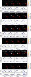 |
Fig. B.3. Same as Figure 3, but with asymmetry and position angle as additional parameters. |
| In the text | |
|
Fig. D.1. Comparison of the RR (orange) and LL (green) closure phases on the ALMA-NOEMA-PV (top) and ALMA-KP-SMT triangles (bottom). The red line indicates the DoG-HIT ring model, the magenta line indicates the DoG-HIT model with an additional Gaussian component. |
| In the text | |
Current usage metrics show cumulative count of Article Views (full-text article views including HTML views, PDF and ePub downloads, according to the available data) and Abstracts Views on Vision4Press platform.
Data correspond to usage on the plateform after 2015. The current usage metrics is available 48-96 hours after online publication and is updated daily on week days.
Initial download of the metrics may take a while.