| Issue |
A&A
Volume 706, February 2026
|
|
|---|---|---|
| Article Number | A104 | |
| Number of page(s) | 18 | |
| Section | Numerical methods and codes | |
| DOI | https://doi.org/10.1051/0004-6361/202557178 | |
| Published online | 04 February 2026 | |
The Modular Computational Simulation Interface (MoCSI) code
I. Thermophysical model for investigating surface environments of small bodies
Institut für Planetologie, Universität Münster,
Wilhelm-Klemm-Str. 10,
48149
Münster,
Germany
★ Corresponding author: This email address is being protected from spambots. You need JavaScript enabled to view it.
Received:
9
September
2025
Accepted:
26
November
2025
Abstract
Context. With many different missions to small bodies and (icy) moons currently ongoing or on the horizon, modern thermophysical models for planetary science need to be able to be adapted to quickly changing parameters and science objectives.
Aims. We aim to develop the public and open-source Modular Computational Simulation Interface (MoCSI) code to offer a fully modular thermophysical model that can be applied to asteroids and to a wide variety of dry, airless bodies in the future. Further, we intend to compare MoCSI to established thermophysical models and show a proof-of-concept application to the Kolobok crater on the asteroid (162173) Ryugu.
Methods. MoCSI employs a finite element method (FEM) to solve the one-dimensional transient heat-transfer equation. Physical variables, for example thermal conductivity, bulk density, or incoming radiative flux, and different model behavior, for example dynamic time-step reduction, can be implemented through modules that the user can turn on and off to suit their science case.
Results. There is good agreement between MoCSI and the two published models 1DTM and heat1d to within < 1 K or <1%. Different treatments of the boundary conditions, especially the surface-energy-balance boundary condition, can lead to differences of >5 % during specific time-steps. The proof-of-concept application showed close agreement with the established literature.
Conclusions. MoCSI’s modular code base allows for rapid adaption, not only to different physical applications, but also to the use of different types of thermophysical models. It can be expanded to refine results and to include new physical descriptions and numerical methods. Ongoing development is planned to further improve performance and expand the available list of modules.
Key words: methods: numerical / minor planets, asteroids: general
© The Authors 2026
 Open Access article, published by EDP Sciences, under the terms of the Creative Commons Attribution License (https://creativecommons.org/licenses/by/4.0), which permits unrestricted use, distribution, and reproduction in any medium, provided the original work is properly cited.
This article is published in open access under the Subscribe to Open model. This email address is being protected from spambots. You need JavaScript enabled to view it. to support open access publication.
1 Introduction
The development of thermophysical models for heat transfer in the surface regions of small bodies, moons, and terrestrial planets has been rapidly progressing in the past few decades (see e.g., Davidsson & Skorov 2002; Gutiérrez et al. 2001; Hayne et al. 2017; Gundlach et al. 2020; Okada et al. 2020; Bauch et al. 2021). However, there is a growing need for advanced thermal models that can be easily adapted to unique characteristics of newly explored bodies. The thermal infrared imager (TIR) aboard the Hayabusa2 spacecraft (Arai et al. 2017), the OSIRIS-REx Thermal Emission Spectrometer (OTES) aboard the OSIRIS-REx spacecraft (Christensen et al. 2018), and the thermal infrared imager (TIRI) aboard the Hera spacecraft (Sect. 5.4 in Michel et al. 2022) are just some recent examples of the plethora of existing thermal mapping endeavors of small bodies or that are on the horizon. The data from the Diviner instrument aboard the Lunar Reconnaissance Orbiter has been used for over a decade to compare with thermophysical models (Paige et al. 2010; Hayne et al. 2017). Looking beyond that, the Europa Clipper and JUICE mission of the Galilean satellites will carry instruments to investigate the thermal structure of Europa’s and Ganymede’s surfaces. While the Europa Thermal Emission Imaging System (E-THEMIS) will fly on board the Europa Clipper spacecraft and will deliver thermal maps of the Jovian satellite (Christensen et al. 2024), JUICE carries a Submillimeter Wave Instrument (SWI) that will investigate the temperature structure of the near surface (Sect. 4.3 in Fletcher et al. 2023). These different use cases all signify the need for easily adaptable, well-performing, and reliable thermal models to quickly react to new discoveries and to investigate gaps in our current theoretical models and predictions.
We developed the Modular Computational Simulation Interface (MoCSI) code in order to facilitate quick and easy adaptability of a thermophysical model code to different environments and scientific cases through the use of independent modules. These modules are designed to “plug” into the code and interface with the solver unit. They can be combined flexibly to represent a wide range of use cases, without requiring extensive familiarisation with a complex code infrastructure. In its current form, the core code and the modules are designed to describe aster-oidal surfaces without regolith compaction in the interior and without ices present in the surface layers. In subsequent releases, additional modules can be added to allow for the simulation of surfaces of other atmosphere-less objects, such as the lunar surface, cometary surfaces, and surfaces of icy moons. The suite of modules published with the initial release of the code is listed in Table 1.
In Sect. 2, we describe the governing equations and numerical discretizations, as well as the MoCSI code infrastructure. Section 3 pertains to the validations we used to test the implementation of the MoCSI code. We specifically focused on comparing to the established thermophysical models 1DTM from Schörghofer & Khatiwala (2024) and heat1D from Hayne et al. (2017). As a proof of concept, in Sect. 4 we describe how we applied MoCSI to the Kolobok crater on Ryugu, and we compare our results with TIR data from the Hayabusa2 mission and those yielded by TPM1 described in Okada et al. (2020). Lastly, we summarize the highlights and provide an outlook into further developments in Sect. 5.
Currently implemented managing modules and sub-modules.
2 The MoCSI model
MoCSI is a modular thermophysical model, which in the current state can solve the one-dimensional heat-transfer equation. We introduce the governing equations and numerical framework in Sects. 2.1 and 2.2. The modularity of the code allows for quick adaptation of MoCSI to different applications. Thus, we especially focus on introducing the code structure and how to employ the modules from a user perspective in Sect. 2.3. Lastly, we list the modules that are available in the version 1.0.0 release of MoCSI in Sect. 2.4.
2.1 Governing equations
As MoCSI’s current focus is the thermal surface environment of dry airless bodies, the governing partial differential equation is the one-dimensional heat conduction equation given by
 (1)
(1)
with the thermal conductivity being k, the heat capacity cp, the density ρ, and possible source or sink terms of the continuous medium Q. In later releases the code could be extended to solve the 3D heat conduction equation, but this is beyond the scope of this work. For most applications of comparing simulated temperatures to remote sensing data, the thermal skin depth is far smaller than the measurement footprint. For applications to shape models, the scale of the facets is also usually larger than the thermal skin depth. Both cases warrant reducing the problem to one dimension (King et al. 2020). The classical boundary conditions for the targeted applications are the surface energy balance as the top domain boundary condition and a constant heat flux as the bottom domain boundary condition:
 (2)
(2)
 (3)
(3)
with the net absorbed solar irradiation  and the Stefan-Boltzmann constant σ, and emissivity, ε, as given by the Stefan-Boltzmann radiation law. Further, A is the bolometric Bond albedo, θ is the solar incidence angle, S⊙ is the solar constant, and rh is the heliocentric distance. In cases with more than one surface facet present and 3D radiative energy transfer, QS is the total incoming radiative flux for a facet. While these three equations are the standard-use case of MoCSI, different boundary conditions are provided in order to facilitate numerical verification and different applications.
2.2 Numerical framework
Many different methods have been applied to solve Eq. (1) in previous thermophysical models (e.g., Gundlach et al. 2020; Schörghofer & Khatiwala 2024; Davidsson 2021 ; Ferziger et al. 2019; Lewis et al. 2004). MoCSI employs a finite-elementmethod (FEM) solver. Since small bodies are usually irregularly shaped and a later expansion to higher dimensions is planned, FEM is particularly well suited to discretizing the spatial derivatives. The implementation follows Lewis et al. (2004) and the Galerkin FEM description therein, which is a special case of the weighted residual approach. In the one-dimensional FEM, the temperatures are discretized within elements containing specific node points, xi, at which the temperatures are calculated, resulting in the discretization equation
 (4)
(4)
where n is the number of nodes within an element, Ni are the so-called basis or shape functions that interpolate the temperature within each element, and T is the resulting approximation to the true temperature value at position x (Lewis et al. 2004). MoCSI currently uses linear elements (n = 2), and thus the shape functions follow a linear interpolation with
 (5)
(5)
 (6)
(6)
where xi is the upper position, Xj is the lower position, and lm = Xj - xi is the length of the m-th element. For linear onedimensional elements, j = i + 1 and m = i. Using higher order polynomials, the discretization allows for higher spatial accuracy, but for the current applications, linear elements have been deemed adequate. While for the thermo-physical model most benefits of the FEM are gained by describing irregular shapes in higher dimensions, the one-dimensional FEM formulation allows for easy incorporation of non-uniform grid spacing and also enables a possible variation of the areas at the nodes within the elements, as shown in Fig. 1.
We approximated the solution to the integral form of the heat transfer equation with the Galerkin method, which is a weighted residual method. It can be expressed through the equation
 (7)
(7)
where wi are the weights, L(T) is the partial differential equation (PDE), and Ω is the domain on which the PDE is defined (Lewis et al. 2004). Let T be a solution to the PDE; it follows that there is a form, L(T) = 0, which fulfills Eq. (7). If T is an approximate solution to the PDE, then  with the residual value R. A weighted residual method minimizes the integral of this residual value multiplied by characteristic weight functions. For the Galerkin method, these weight functions are the corresponding nodal shape functions. If we choose the transient heat conduction equation as the PDE L(T) and set the weight functions to the shape functions, we arrive at
 (8)
(8)
With the approximation defined in Eq. (4), integrating by parts and rearranging the terms leads to the well-known form
 (9)
(9)
with the capacitance matrix, C; the stiffness matrix, K; the forcing vector, f; and the vector of temperatures at all nodes, T (Lewis et al. 2004, Eqs. (6.12)-(6.16)). For the case of constant physical parameters and linear shape functions, for each element these values equate to
 (10)
(10)
 (11)
(11)
 (12)
(12)
with the element length lm and the arithmetic mean area Am+1/2 = (Am + Am+1)/2. The arithmetic mean area is used due to the heat flux through the area between nodes being the governing variable, which is best represented by the arithmetic mean for linear elements of different areas. In the case of temperature-dependent and nonlinear temperature dependency parameters, an iterative scheme is applied to solve the equation. In this case, the current time step is repeated iteratively while using the temperatures from each inner iteration for the temperature-dependent or nonlinear thermal parameters. The iterations are performed until a user-defined convergence criterion is reached or a user-set maximum iteration number is reached; however, the user is warned in that case that no convergence was reached. For the temporal discretization, MoCSI uses a finite-difference fully implicit scheme, so the fully discretized heat conduction equation reads
 (13)
(13)
To discretize the surface energy balance boundary condition at the top domain boundary, a linearization of the Stefan-Boltzmann radiation term was performed in order to retain a linear system of equations for the cases in which no temperaturedependent physical parameters were used. We linearized around the surface temperature of the last known time step to obtain
 (14)
(14)
with  and
and  . The resulting matrix elements read
 (15)
(15)
 (16)
(16)
 (17)
(17)
The capacitance matrix elements of the first row have to be set to zero in order to retain the shape of Eq. (2). Due to the temperature dependence of the Stefan-Boltzmann term, its prefactor has to be added to the upper left entry of the stiffness matrix. Substituting these matrices into Eq. (13) yields Eq. (2) for the top temperature in case of no source or sink terms.
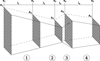 |
Fig. 1 Example of possible FEM grid in one dimension consisting of five nodes at positions xi, with areas Ai making up four linear elements of length, lm. The length between elements and the area at the position of the nodes do not have to be uniform. |
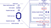 |
Fig. 2 Visualization of core-code capabilities and standard time-stepping loop of MoCSI. Optionally executed functionality is marked as (opt.). The core code mainly provides utilities needed for the simulations. It loads shape models, generates the grid from user specifications, loads and creates snapshots as restoration points, and provides infrastructure such as matrices and solvers for linear systems of equations. The time-stepping loop is shown in detail. It consists of the outer time-integration loop and an inner iteration loop, which is used when nonlinear terms are present within the equations. If active, the steps marked in red are executed, and a check of the change in temperature against a user-specifiable abort criterion, ε, is done after every inner iteration; if the difference is larger than this criterion, it is redone, but with the modules in the pre-time step having access to the previously calculated temperatures. |
2.3 Code structure
The core tenet of MoCSI is full modularity and customizability, allowing for broad applications to planetary science cases. Instead of needing multiple rewrites of core components when using MoCSI for different cases, the goal was to design a code where the addition of new components does not necessitate changes to the core parts of the code. To achieve this, MoCSI’s code consists of two larger sections, the core and the modules. The core comprises the solver, grid generation, shape-function management, input and output processing, and the simulation framework that orchestrates the execution sequence. A more detailed depiction of the structure of the core code is given in Fig. 2. Modules extend the core’s functionality and are managed through a module framework that handles loading, dependency resolution, and overall module management. Current modules include representations of physical parameters, self-heating calculations for realistic surface-boundary conditions, and SPICE kernels (Acton 1996) to simulate realistic illumination conditions, among others (see Table 1). This general core-module structure was inspired by the structure of the GAIA code (Hüttig et al. 2023).
Modules come in two types: managing modules and sub-modules. Managing modules directly interface with the simulation framework in the core code by passing their field parameter. The field parameter of each managing module varies with context; for example, the thermal conductivity for physical parameters, the solar irradiation for self-heating, or the solar vector and heliocentric distance for SPICE kernels.
Sub-modules are required if the field parameter of a managing module can be computed in multiple ways. For instance, there are several models for the thermal conductivity. In such cases, sub-modules perform the actual calculation of the field parameter. If only a single method exists for calculating the field parameter, the managing module can perform the calculation itself. Architecturally, sub-modules do not interface directly with the core, they communicate exclusively with their managing module. Sub-modules can have their own sub-modules, if the calculation can be further divided into smaller sub-calculations. For example, heat conduction in a two-layered subsurface, where these layers consist of separate materials, requires separate thermal-conductivity descriptions for each layer. This hierarchy is implemented via sub-sub-modules. In this example, the managing module defines the field parameter: thermal conductivity. The first layer of sub-modules determines how thermal conductivity is assigned, distributing values to the two sub-surface layers. The second layer of sub-modules then calculates the actual conductivities for each layer. The user selects the material type for each layer by loading the corresponding thermal conductivity descriptions as the sub-sub-modules.
Users can configure their set of modules to fit their scientific use case and insert them into MoCSI’s core at fixed “module insertion points”. These allow the evaluation of modules, i.e., the computation of their field parameter, at key stages of the simulation. The key stages are listed below.
Initialization: before the time loop when parameters are first set.
Pre-time step: at the start of each nonlinear iteration within a time step, before temperature values are updated.
Post-nonlinear iteration: after each iteration within the timestepping loop (only needed for nonlinear PDEs).
Post-time step: at the end of each time step within the loop, after the iterations have converged.
Output: after the time loop of the simulation has ended.
This design provides a structured framework for user interaction. Furthermore, each module insertion point can have its own unique set of modules, thus giving the user a high degree of flexibility and adaptability across different scientific use cases.
2.4 Available modules
The modules that must always be loaded are those representing physical parameters in the heat conduction equation: the density, heat capacity, thermal conductivity, and source- and sink-term modules. An additional module for solar irradiation is required if a surface energy balance is used as a boundary condition (see Eq. (2)). Different sub-modules with specific implementations are already available for each of these modules. A list of all currently available modules is given in Table 1.
A special module is the SolarFluxVariable-Potter2023Radiosity module. It enables three-dimensional radiative-energy transfer on a given shape model using the radiosity equations to calculate the total flux each facet receives (Potter et al. 2023). Ray casting is employed to correctly calculate self-heating and shadowing effects and can be combined with the HeliocentricDistanceVariableSpice and SolarVectorVariableSpice modules to include SPICEbased insolation-condition calculations. While it currently only works with a bolometric Bond albedo, it can be expanded to work with incidence-angle-dependent albedos, as needed for descriptions of the lunar surface, for example (Keihm 1984; Foote et al. 2020).
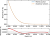 |
Fig. 3 Temperature profiles comparing results of MoCSI code with an analytical solution given by Eq. (18), and residuals between both solutions. The MoCSI results were produced for a spatial resolution of 5 ∙ 10−5 m and a temporal resolution of 10−4 s after 1 s of simulation time. |
3 Validation
We benchmarked MoCSI by comparing it to three different solutions. As a baseline validation for our solver, we first used a known analytical solution to the heat-transfer equation and as a convergence test in Sect. 3.1. To specifically test our implementation of the surface energy balance, we compared MoCSI and the default test case of the 1DTM model by Schörghofer & Khatiwala (2024) and Schörghofer (2025) in Sect. 3.2, and the heat1D model by Hayne et al. (2017) in Sect. 3.3. Lastly, we show a comparison of our radiosity code to the analytical solution of the irradiation of a spherical crater provided by Ingersoll et al. (1992) in Sect. 3.4. The parameters used for each validation simulation are given in Appendix A.
3.1 Comparison to an analytical solution
We used an analytical solution of the heat-conduction equation with von Neumann boundary conditions to test the implementation of our solver. For a semi-infinite domain with a constant heat flux at the top and no flux at the bottom, the solution is given in Incropera et al. (1996, Eq. (5.59)) as
 (18)
(18)
with the starting temperature of the entire domain, Tinitial; the constant surface-heat flux, q0; the thermal diffusivity,  ; and the complementary error function, erfc (x).
The physical parameters and timescale have been chosen to ensure that the heat does not reach the bottom of the 3 cm simulated domain, so as to keep the temperature differences at the bottom due to the finite domain minimal. The numerical results generated with MoCSI were computed with a uniform element length of 5 ∙ 10−5 m and a time-step resolution of 10−4 s. Figure 3 compares the numerical results after 1 s of simulation with the analytical results. We further verified the expected convergence orders of O (∆t) and O ((∆x)2). Figure 4 shows the discrete L2 norm error against the spatial and temporal step sizes. As expected for a backward Euler time-stepping scheme, the temporal error converges at first order. The spatial error shows second-order convergence, which is consistent with linear FEM elements.
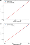 |
Fig. 4 Convergence analysis of MoCSI code for the comparison against the analytical solution given by Eq. (18). Panel a: spatial convergence shown by plotting L2 error against element length. Panel b: temporal convergence shown by plotting L2 error against time-step length. Power-law fits for both plots have been produced, verifying that both the temporal and spatial convergence show the expected slopes of 1 and 2, respectively. |
3.2 Comparison to 1DTM
To validate our implementation of the surface energy balance as a possible boundary condition, we compared our results to the ones produced by the “common” program from the Planetary Code Collection of Norbert Schörghofer (Schörghofer & Khatiwala 2024; Schörghofer 2025), which we refer to as 1DTM hereafter. The authors provided a text file with the results of a specified test run for their internal validation, which we compared our code to. We configured MoCSI to closely resemble the parameters in the 1DTM code. All physical parameters were set to the same values, the surface energy balance was set as the top boundary condition, and a fixed geothermal heat flux of 0.2 W m−2 was set as the bottom boundary condition. The solar flux was calculated in both models using sinusoidal day-night cycles for a single facet on a spherical body with a possible slope against the surface normal (see Eqs. (2.1)-(2.3) in the user guide of Schörghofer 2025). Finally, we implemented the artificial flux-smoothing condition described in Schörghofer & Khatiwala (2024) as a module. Note that we did not implement the available Volterra predictor. The MoCSI core code uses iterations to treat nonlinearities within the equations. Using the Volterra predictor would require changes to the core code, which are not intended. Furthermore, Schörghofer & Khatiwala (2024) already showed the equivalence of these methods to within a few percent.
We see an excellent agreement, i.e., ∆ Tmax < 1K or ∆Tmax,rel < 1%, during both day and night time between 1DTM and MoCSI (see Fig. 5), with
 (19)
(19)
 (20)
(20)
There is a notable difference between the models during sunrise and sunset with differences up to ∆Tmax = 5.8 K or ∆Tmax,rel < 5.6%. This is expected, as the Volterra predictor used in Schörghofer & Khatiwala (2024) is not implemented in MoCSI. Schörghofer & Khatiwala (2024) show that using different implementations to predict the surface temperature leads to differences of a few Kelvin, which explains the differences observed here. The surface-temperature differences during sunrise and sunset propagate inward over time, producing the wavy pattern in the residuals. Beyond these transition periods, the two models are in good agreement with each other, confirming that our implementation of the boundary condition is adequate.
3.3 Comparison to heat1d
We also compared MoCSI to the heat1d thermal model by Hayne et al. (2017). The Python version of said model contains a testing notebook, to which we chose to compare our results. A characteristic of the heat1d model is the equilibration phase of the model, where one orbit is simulated for the chosen body in order to generate an equilibrium temperature profile from which the main simulation will start.
Figure 6 shows the comparison of MoCSI with the solutiontemperature profile of heat1d for the physical parameters resembling Ganymede. The differences between MoCSI and heat1d are on the order of ∆ Tmax ≃ 1 K for the interior and ∆ Tmax ≃1.9 K for the upper boundary condition or ∆Tmax,rel ≃ 2.6% and ∆Tmax,rel ≃ 5.0%, respectively. The differences for the interior points arise from two factors: the models treat the terms differently, and they evaluate the depth-dependent thermal properties at different positions within the grid. The heat conductivity is calculated at the interface between two nodes in MoCSI, while it is calculated directly on the node in heat1d. Further, MoCSI employs an iterative scheme to deal with nonlinear thermal properties, while this heat1d version does not. Both the iterations in all temperatures and the interface heat conductivity lead to a more effective heat transport from the lower boundary to the interior points, which explains the slightly lower temperatures of MoCSI.
The differences for the surface temperature due to differences in the treatment of the upper boundary condition are more complex, because heat1d uses an iterative procedure to calculate that specific temperature. While the factors affecting interior points - as discussed above - also influence the boundary points, the primary contributor to differences at the upper boundary is the discretization of the heat conduction term in the surface energy balance. The heat1d discretization of the heat conduction term reads
 (21)
(21)
employing a three-point discretization for the differential. In this term, both the heat conductivity and the two values T1 and T2, which are not iterated, could lead to differences between the heat1d implementation and the MoCSI implementation.
To approximate the change in temperatures these implementation differences yield, we altered the heat1d iterative scheme both with the known T1 and T2 temperature values from the next time step, as well as with an interface heat conductivity implementation. We ran the now-altered heat1d surface-temperature evaluation again and compared these new values with the unaltered heat1d values, as shown in Fig. 7. It can be seen that both changes can lead to differences of up to 4 K, when compared to the unaltered implementation. This leads to the conclusion that the differences in the surface-energy balance between the two models are purely implementation dependent, and within these differences, they do agree with each other. It should be noted that this is only a rough estimation, as the T1 and T2 values are still not iterated, but simply taken from the next time step of the default model. While these results would still change in a fully iterative heat1d implementation, the first iteration is commonly the one with the largest impact on the temperature profile; we expect the differences to stay in this magnitude.
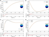 |
Fig. 5 Selected temperature profiles showing comparison between MoCSI code and 1DTM code at different times; i.e., the first time step after sunrise (panel a), the time step closest to noon (panel b), the first time step after sunset (panel c), and the time step closest to midnight (panel d). The differences during sunrise and sunset can be explained by the difference in surface-temperature prediction scheme, as also discussed in Schörghofer & Khatiwala (2024). Away from the boundary, where gradients are less steep, the two implementations show good agreement. Since surface temperatures differ slightly between the models, these differences propagate downward with the thermal profile. This explains the wavy structure in the residuals. |
3.4 Validation of the radiosity equations
When using topographic information through a shape model with more than one facet, these facets can interact with each other via energy-flux exchange. Most commonly, three types of fluxes are encountered: (1) direct insolation from a light source; (2) indirect insolation through scattered light; and (3) thermal radiation from the topography, which is depicted in Fig. 8. In most equatorial configurations and on flat topographies, (1) is the most dominant term, but in polar regions and on cratered or rocky topographies, the influence of (2) and (3) are non-negligible. The radiosity equations describe the energy transfer between topographic elements in the presence of all three fluxes (Potter et al. 2023). MoCSI implements the radiosity equations following the description of Potter et al. (2023). To validate the implementation, we used their spherical crater mesh to compare the simulated temperatures to the analytical solution of the radiative-heat transfer in a bowl-shaped crater from Ingersoll et al. (1992). The solution for a bowl-shaped crater with a solar incidence angle can be transcribed as
 (22)
(22)
with the solar incidence angle i⊙ between the plane and the sun, the incidence angle between the sun and a facet, i; the albedo A; and the geometric factor b = f (ε + A) (1 - f) / (1 - Af), where 1/f = 1 + 1/4 ∙ D2∕d2 is dependent on the crater diameter-to-depth ratio, D/d (see also Fig. 1a in Potter et al. 2023).
We used MoCSI to compute the view-factor matrix elements and insolation at each facet. These were then used to calculate the facet temperatures, which are compared to the analytical solution. The result is shown in Fig. 9. It depicts the top-down view onto a three-dimensional model of a spherical crater with 14 198 facets (see also Fig. 1b in Potter et al. 2023). While Fig. 9a illustrates the absolute temperature inside the crater modeled by MoCSI, Fig. 9b highlights the difference between the analytical solution and the MoCSI results. Residuals are higher on the shadowed side (<1 K) than on the sunlit side (<0.1 K) due to the different contributions of the radiative fluxes. On the shadowed side, infrared emissions and reflected light from the sunlit facets are the only contributions, making it more sensitive to simplifications in the method and approximations in the crater geometry. By contrast, the sunlit side is dominated by the incoming solar flux, so the influence of approximations is minimal. The remaining discrepancies with the analytical solution arise from using the far-field approximation within the view-factor calculation and the finite-mesh discretization, which can be reduced by increasing the number of facets.
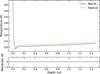 |
Fig. 6 Temperature profiles comparing results of MoCSI code with heat1d results and residuals between both models. An explanation for the differences between the models is given in Fig. 7. |
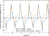 |
Fig. 7 Temperature differences between standard heat1d implementation of surface-temperature calculation and two other implementations. The implementation represented by the blue line uses the temperatures of the next time step to approximate the temperature differential in the boundary condition. The implementation represented by the dashed orange line also uses the temperatures of the next time step and also calculates the heat conductivity at the interface between two grid points instead of directly at the points. While this is only a rough approximation of the changes a fully iterative heat1d would produce, it shows the general difference in temperatures we can expect from the changes to be in the low-Kelvin range. |
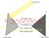 |
Fig. 8 Visualization of energy transfer between two facets described through radiosity equations. Light from a given source directly illuminates one facet, which scatters the light to other topography that in return can scatter this light again. Furthermore, both facets have an associated temperature and thermal emission of infrared radiation, which they can transfer between each other. These three types of fluxes are represented within the radiosity equations. |
4 Application to Ryugu’s Kolobok crater
As a proof of concept, we applied MoCSI to a more complex three-dimensional geometry; for this, we chose the Kolobok crater on the asteroid (162173) Ryugu. The Kolobok crater is a large, central crater (240 m, 1.5° S) on the equatorial ridge of Ryugu (Sugita et al. 2019). It is thus well suited to be simulated in isolation without the need to consider large surrounding regions of Ryugu’s surface to correctly model radiosity. Such a quasiisolated environment is necessary as simulations on the full shape model are beyond the scope of this work. Future updates of MoCSI are planned to involve parallelization of the code facilitating computations on full shape models. We compared the results to the TIR l3 dataset acquired by the TIR instrument during the Hayabusa2 mission (Watanabe & Kikuchi 2024) and simulation results of Okada et al. (2020) - another thermophysical model utilized to calculate surface temperatures on Ryugu.
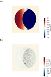 |
Fig. 9 Top-down view of three-dimensional model of spherical crater with 14 198 facets, partially lit by the sun at a 15° incidence angle. Panel a: simulated surface temperatures. Panel b: differences between the analytical solution in Eq. (22) and simulated temperatures. While the residuals in the shadowed region reach up to ≲1 K, on the sunlit side they are around ≲0.1 K and below. |
4.1 MoCSI configuration
MoCSI was run with a constant bulk density, specific heat capacity, thermal conductivity, albedo, and emissivity in order to compare our results to those of Okada et al. (2020). The values used are given in Table 2. The bulk density was taken from measurements during the Hayabusa2 mission (Nakamura et al. 2022), and the specific heat capacity was taken from the proxy material serpentine (Osako et al. 2010). The thermal conductivity was calculated to equate to a thermal inertia of 300 Jm−2K−1 s−1/2, which was the best-fitting value of Okada et al. (2020), to better compare our simulation. While this results in a low thermal conductivity, it is within the range of thermal conductivities measured from the returned Ryugu samples in vacuum conditions (Ishizaki et al. 2023). Further, we tested the influence of temperature dependency on the thermal conductivity and specific heat capacity values. A discussion of this influence is given in Appendix D.
Our model region spans the Kolobok crater and rim region on the low-resolution stereophotoclinometry (SPC) shape model of Watanabe et al. (2019). We simulated one orbit, corresponding to 474.729 earth days (Watanabe & Kikuchi 2024), to allow for equilibration of the deeper temperatures. For this, we employed a temporal resolution of 20 time steps per one Ryugu day (7.6326 hours; Watanabe & Kikuchi 2024). After equilibration, we simulated a single day with a resolution of 10 s per time step. To compare our results to the findings of Okada et al. (2020), who compared their model to the TIR dataset from the global mapping done on 1 Aug 2018, we chose to simulate the same day.
Thermal parameters and sources.
4.2 Results
The simulated surface temperatures and the comparison to the measured and mapped TIR brightness temperatures (TIR l3 dataset) are shown in Fig. 10. We compared the simulated temperatures at 1 Aug 2018 18:16:30 with the measured and mapped TIR brightness temperatures at 1 Aug 2018 18:16:32 (all times UTC). On average, the temperatures of the simulation are higher (in the range of 10-20 K) than the TIR brightness temperatures.
This result is in agreement with the simulations done by Okada et al. (2020, their Fig. 2) for the same TIR dataset. They saw almost exclusively higher simulated temperatures in the same range of 10-20 K, except for the top left rim of the crater, which MoCSI confirms.
We also compared the simulated temperatures to the TIR observations at several times during the same day. For each facet i and each observation time (corresponding to one TIR image), the difference was calculated as ∆Ti = Ti,TIR - Ti,MoCSI. Figure 11 shows, for each point in time, the median temperature differences across all facets within the Kolobok crater. The error bars indicate the spread of facet-wise differences, given by the 10th-90th percentile range. The gap in the data between 11:00 and 17:00 reflects both missing TIR acquisitions and the exclusion of observations in which, relative to the shape-model discretization, fewer than half of the Kolobok crater facets were observed.
While these results support the previous finding (see Fig. 10) of higher simulated temperatures at 2018-08-01T18:16:30, they additionally reveal that simulation temperatures are generally hotter than TIR observations at low solar incidence angles and colder than TIR observations at high solar incidence angles.
This might be explained by the high surface roughness on Ryugu, which was discussed in Shimaki et al. (2020). The authors concluded that surface roughness could lower the noon temperatures and increase the sunset and sunrise temperatures compared to their current simulations, which is the same pattern we see in our simulation. A corresponding surface-roughness module is expected to be added in a future update. Another influence could be a steep increase of Albedo for large solar-incidence angles, i.e., the limb-brightening effect, which has been observed for airless bodies, most prominently for the Moon (Keihm 1984).
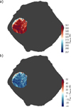 |
Fig. 10 Simulated temperatures and temperature differences between simulation and TIR measurements. Panel a: simulated surface temperatures within the Kolobok crater at 1 Aug 2018 18:16:30 UTC. Panel b: differences between measured and mapped TIR temperatures and the simulated temperatures. The TIR measurement was taken at 1 August 2018 18:16:32 UTC. The dark gray regions of Ryugu were not simulated. The absolute median difference between the TIR temperature and the simulated temperature is 16 K, with the simulated temperatures being hotter. |
5 Conclusions and future prospects
We introduce the Modular Computational Simulation Interface code, MoCSI, which was written with adaptability and ease-of-use in mind.
We show that the solver employed by MoCSI reproduces analytical solutions and provides the expected convergence behavior. We conducted a comparison between MoCSI and the 1DTM code from Schörghofer & Khatiwala (2024), as well as the heat1d code from Hayne et al. (2017). The comparison showed that while the models all generally agree with each other to within ∆Tmax,rel < 1%, the chosen discretization and linearization of the surface energy balance can introduce differences between the models of ∆Tmax,rel > 5%. While observed differences are moderate and only significant during a few time steps, it is important to acknowledge these uncertainties, especially when trying to match simulations at specific conditions and points in time.
Lastly, we investigated surface temperatures in the Kolobok crater of the asteroid (162173) Ryugu as a proof-of-concept study. The direct comparison to the TIR l3 dataset showed that the simulated surface temperatures at 2018-08-01T18:16:32 were 10-20 K hotter than the brightness temperatures measured by TIR. This matched well with the simulations of Okada et al. (2020), which also showed higher temperatures in the Kolobok crater. We agree with the authors’ interpretation that the observed effect may result from surface roughness, a point further elaborated in Shimaki et al. (2020).
A surface-roughness module is currently being developed in order to achieve a better fit between observed and modeled temperatures. Incorporating surface roughness requires careful treatment and is thus beyond the scope of this paper.
MoCSI is publicly available under GNU General Public License v3 through the Git repository1 or the Zenodo repository2. It will be further developed by adding more modules and by improving the core code; this can be done by adding more efficient solvers and by implementing code parallelization, for example. We envision that different module combinations can be used in the future to simulate various atmosphere-less objects of the Solar System, such as asteroids, comets, icy moons and the Moon. Therefore, multiple modules can be added to the code framework, such as those listed below.
Surface-roughness module
Gas-diffusion module and solver update (coupling of two differential equations)
Water-ice module (sublimation, sintering, etc.)
Compaction of surface layers module.
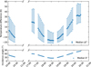 |
Fig. 11 Median temperature differences between the TIR temperatures and the simulated temperatures of all facets in the Kolobok crater for the global temperature mapping done for 1 August 2018 (all times UTC; Okada et al. 2020). The error bars indicate the range of the 10th and 90th percentiles of temperature differences on the 907 facets used for the simulation. The bottom panel shows the median incidence angle of all facets visible to TIR at the given time. A gap in the data between 10:30 and 14:00 exists and only points are used where more than 453 facets of the employed shape model were seen by TIR, which widens the data gap up to 17:00. |
Data availability
The version of code that was used to generate the results presented in this paper is publicly available in the Zenodo repository https://doi.org/10.5281/zenodo.17062991 or the Git repository https://gitlab.git.nrw/uni-ms/ag-gundlach/public/mocsi under the v1.0.0 tag and the release tab.
Acknowledgements
BA is supported by the Co-Sponsored Research Agreement “Regolith Intelligence: ISRU Prepping with machine learning research on lunar rocks” (4000142823) with the European Space Agency (ESA) and by a Sofja Kovalevskaja Award of the Alexander von Humboldt Foundation.
References
- Acton, C. H. 1996, Planet. Space Sci., 44, 65 [Google Scholar]
- Arai, T., Nakamura, T., Tanaka, S., et al. 2017, Space Sci. Rev., 208, 239 [Google Scholar]
- Arnold, N. S., Rees, W. G., Hodson, A. J., & Kohler, J. 2006, J. Geophys. Res.: Earth Surf., 111 [Google Scholar]
- Bauch, K. E., Hiesinger, H., Greenhagen, B. T., & Helbert, J. 2021, Icarus, 354, 114083 [NASA ADS] [CrossRef] [Google Scholar]
- Christensen, P. R., Hamilton, V. E., Mehall, G. L., et al. 2018, Space Sci. Rev., 214, 87 [Google Scholar]
- Christensen, P. R., Spencer, J. R., Mehall, G. L., et al. 2024, Space Sci. Rev., 220, 38 [Google Scholar]
- Davidsson, B. J. R. 2021, MNRAS, 505, 5654 [NASA ADS] [CrossRef] [Google Scholar]
- Davidsson, B. J. R., & Skorov, Y. V. 2002, Icarus, 159, 239 [CrossRef] [Google Scholar]
- Ferziger, J. H., Perić, M., & Street, R. L. 2019, Computational Methods for Fluid Dynamics, 4th edn. (Cham: Springer) [Google Scholar]
- Fletcher, L. N., Cavalié, T., Grassi, D., et al. 2023, Space Sci. Rev., 219, 53 [Google Scholar]
- Foote, E. J., Paige, D. A., Shepard, M. K., Johnson, J. R., & Biggar, S. 2020, Icarus, 336, 113456 [Google Scholar]
- Gundlach, B., & Blum, J. 2013, Icarus, 223, 479 [Google Scholar]
- Gundlach, B., Fulle, M., & Blum, J. 2020, MNRAS, 493, 3690 [NASA ADS] [CrossRef] [Google Scholar]
- Gutiérrez, P. J., Ortiz, J. L., Rodrigo, R., & López-Moreno, J. J. 2001, A&A, 374, 326 [CrossRef] [EDP Sciences] [Google Scholar]
- Hamm, M., Grott, M., Senshu, H., et al. 2022, Nat. Commun., 13, 364 [NASA ADS] [CrossRef] [Google Scholar]
- Hayne, P. O., Bandfield, J. L., Siegler, M. A., et al. 2017, J. Geophys. Res.: Planets, 122, 2371 [Google Scholar]
- Hüttig, C., Plesa, A.-C., & Tosi, N. 2023, GAIA [Google Scholar]
- Incropera, F. P., DeWitt, D. P., Bergman, T. L., & Lavine, A. S. 1996, Fundamentals of Heat and Mass Transfer, 6 (Wiley New York) [Google Scholar]
- Ingersoll, A. P., Svitek, T., & Murray, B. C. 1992, Icarus, 100, 40 [NASA ADS] [CrossRef] [Google Scholar]
- Ishiguro, M., Kuroda, D., Hasegawa, S., et al. 2014, ApJ, 792, 74 [Google Scholar]
- Ishizaki, T., Nagano, H., Tanaka, S., et al. 2023, Int. J. Thermophys., 44, 51 [NASA ADS] [CrossRef] [Google Scholar]
- Keihm, S. J. 1984, Icarus, 60, 568 [Google Scholar]
- King, O., Warren, T., Bowles, N., et al. 2020, Planet. Space Sci., 182, 104790 [Google Scholar]
- Lewis, R. W., Nithiarasu, P., & Seetharamu, K. N. 2004, Fundamentals of the Finite Element Method for Heat and Fluid Flow (John Wiley & Sons, Ltd) [Google Scholar]
- Maxwell, J. C. 1873, Clarendon Press, 2, 3408 [Google Scholar]
- Michel, P., Küppers, M., Bagatin, A. C., et al. 2022, PSJ, 3, 160 [NASA ADS] [Google Scholar]
- Miyazaki, A., Yada, T., Yogata, K., et al. 2023, Earth Planets Space, 75, 171 [NASA ADS] [CrossRef] [Google Scholar]
- MOOSE Framework 2025, MOOSE Framework verification with analytical solution [Google Scholar]
- Morota, T., Sugita, S., Cho, Y., et al. 2020, Science, 368, 654 [NASA ADS] [CrossRef] [Google Scholar]
- Nakamura, E., Kobayashi, K., Tanaka, R., et al. 2022, Proc. Jpn. Acad. Ser. B, 98, 227 [Google Scholar]
- Okada, T., Fukuhara, T., Tanaka, S., et al. 2020, Nature, 579, 518 [NASA ADS] [CrossRef] [Google Scholar]
- Opeil, C. P., Britt, D. T., Macke, R. J., & Consolmagno, G. J. 2020, Meteor. Planet. Sci., 55, E1 [Google Scholar]
- Opeil, C. P., Consolmagno, G. J., & Britt, D. T. 2010, Icarus, 208, 449 [NASA ADS] [CrossRef] [Google Scholar]
- Osako, M., Yoneda, A., Ito, E., et al. 2010, Phys. Earth Planet. Interiors, 183, 229 [Google Scholar]
- Paige, D. A., Foote, M. C., Greenhagen, B. T., et al. 2010, Space Sci. Rev., 150, 125 [Google Scholar]
- Patankar, S. V. 1980, Numerical Heat Transfer and Fluid Flow (Hemisphere Publishing Corporation) [Google Scholar]
- Potter, S. F., Bertone, S., Schörghofer, N., & Mazarico, E. 2023, J. Computat. Phys.: X, 17, 100130 [Google Scholar]
- Reynard, B., Hilairet, N., Balan, E., & Lazzeri, M. 2007, Geophys. Res. Lett., 34, L13307 [Google Scholar]
- Schörghofer, N. 2025, Planetary-Code-Collection: Thermal, Ice Evolution, and Exosphere Models for Planetary Surfaces [Google Scholar]
- Schörghofer, N., & Khatiwala, S. 2024, PSJ, 5, 120 [Google Scholar]
- Shimaki, Y., Senshu, H., Sakatani, N., et al. 2020, Icarus, 348, 113835 [Google Scholar]
- Sugita, S., Honda, R., Morota, T., et al. 2019, Science, 364, eaaw0422 [Google Scholar]
- Watanabe, S., & Kikuchi, S. 2024, Asteroid Ryugu and the Hayabusa2 Mission [Google Scholar]
- Watanabe, S., Hirabayashi, M., Hirata, N., et al. 2019, Science, 364, 268 [NASA ADS] [Google Scholar]
- Yokoyama, T., Nagashima, K., Nakai, I., et al. 2023, Science, 379, abn7850 [NASA ADS] [CrossRef] [Google Scholar]
Appendix A Parameters for the validation runs
For the sake of completeness, a list of physical parameters used for the validations of MoCSI presented in this paper shall be given here in Table A.1.
Physical parameters used in the validation of MoCSI and comparison to 1DTM and heat1D.
Appendix B All time step comparisons to the 1DTM code
In Schörghofer (2025), the author provided a file of temperature profiles containing the profiles of 13 time steps for internal verification. We have used them to produce the comparison shown in Fig. 5, but only showed the significant results. Here, we show the remaining 8 plots for the full comparison. We have omitted the 13th profile, as it is equivalent to the first profile, for one day-night-cycle within the given default case is spanning 12 time steps.
 |
Fig. B.1 Selected temperature profiles showing the comparison between the MoCSI code and the 1DTM code. One row shows the two time steps that are between the ones shown in Fig. 5 in progressing time. |
Appendix C Description of available MoCSI modules and module structure
This section expands on Table 1 and more thoroughly describes available modules in the version 1.0.0 release of MoCSI. Further, it shows illustrations detailing the module-submodule structure and module insertion points.
Appendix C.1 Detailed module descriptions
Albedo: This managing module represents the variable of the bolometric directional-hemispherical albedo A, with (1 - A) representing the fraction of incoming radiative flux that is absorbed by a surface. The variable field is of the size of the number of facets of the used shape model or 1 if none is used.
AlbedoConstantCustom: This submodule uses a user-supplied bolometric directional-hemispherical albedo value which is kept constant throughout the entire simulation.
Density: This managing module represent the variable of the bulk density ρ of a numerical layer in the simulation domain. The variable field is of size of the number of facets times the number of numerical layers.
DensityConstantCustom: This submodule uses a user-supplied bulk density value which is kept constant throughout the entire simulation.
DensityConstantGundlach2013RegolithSolidAsteroidType: This submodule uses the measurements of the density of various meteorites performed by Opeil et al. (2010) to provide the bulk density of S, Q, M, and C type asteroids. To derive the bulk density from the grain values given in the paper, they are multiplied by a user specified volume filling factor, but are otherwise kept constant throughout the entire simulation.
Emissivity: This managing module represents the mid-infrared emissivity of a surface. The variable field is of the size of the number of facets of the used shape model or 1 if none is used.
EmissivityConstantCustom: This submodule uses a user-supplied mid-infrared emissivity value which is kept constant throughout the entire simulation.
FluxSmoothingTool: This managing module recreates the flux smoothing behavior of the 1DTM code. The user can specify an upper and lower threshold as a factor and if the temperature of the current time step either overshoots the temperature of the previous timestep times the upper threshold or undershoots the temperature of the previous timestep times the lower threshold, it redoes the time step with 5 time steps of size dt/5. It does not represent a variable field.
HeatCapacity: This managing module represent the variable of the bulk specific heat capacity cp of a numerical layer in the simulation domain. The variable field is of size of the number of facets times the number of numerical layers.
HeatCapacityConstantCustom: This submodule uses a user-supplied bulk specific heat capacity value which is kept constant throughout the entire simulation.
HeatCapacityConstantOpeil2010NonPorousRockSolidAsteroidType: This submodule uses the measurements of the specific heat capacity of various meteorites performed by Opeil et al. (2010) to provide the bulk specific heat capacity of S, Q, M, and C type asteroids. The reported values at 200 K are used and are kept constant throughout the entire simulation, as the authors did not report the temperature dependence of these values.
HeatConductivity: This managing module represent the variable of the bulk thermal conductivity k of a numerical layer in the simulation domain. As the thermal conductivity is an interface variable Patankar (1980), it is calculated at the interface between two nodes, instead of at the nodes. The variable field is of size of the number of facets times the number of numerical layers.
HeatConductivityConstantCustom: This submodule uses a user-supplied bulk thermal conductivity value which is kept constant throughout the entire simulation.
HeatConductivityConstantMaxwell1873PorousRockSolid: This submodule uses the thermal conductivity model of Maxwell (1873) to calculate the bulk thermal conductivity of a porous rock from the solid thermal conductivity of the material and the volume filling factor. The solid thermal conductivity needs to be supplied by another submodule. Whether the calculated value is constant or not depends on the submodule used.
HeatConductivityTwoLayers: This submodule combines the thermal conductivity of two submodules, by using one of the thermal conductivity values for the upper region an the other value for the lower region. The user can specify which module should be used in the upper and lower region and at which numerical layer the boundary of the regions should be. Whether the calculated value is constant or not depends on the submodules used.
HeatConductivityVariableGundlach2013NonPorousRockSolidAsteroidType: This submodule uses the measurements of the solid material thermal conductivity of various meteorites to provide the solid material thermal conductivity of S, Q, M, and C type asteroids (Gundlach & Blum 2013). While the S and Q type values are constant, the M and C type values are temperature and thus depth and time dependent.
HeatConductivityVariableGundlach2013RegolithSolid: This submodule uses the thermal conductivity model of Gundlach & Blum (2013) to calculate the bulk thermal conductivity of regolith from the solid thermal conductivity of the material, the volume filling factor, the temperature and various material properties. The solid thermal conductivity needs to be supplied by another submodule. It is explicitly temperature dependent through a radiative heat conductivity term and thus always depth and time dependent.
HeatSource: This managing module represent the variable of the heat source and sink terms Q within a numerical layer in the simulation domain. The variable field is of size of the number of facets times the number of numerical layers.
HeatSourceConstantCustom: This submodule uses a user-supplied heat source or sink value which is kept constant throughout the entire simulation.
HeliocentricDistance: This managing module represent the variable of the normalized heliocentric distance R⊙/1 AU, the distance between the sun and the simulated object, which is used for calculating incoming solar flux when using the surface energy balance boundary condition. The variable field is always of size 1.
HeliocentricDistanceConstantCustom: This submodule uses a user-supplied heliocentric distance which is kept constant throughout the entire simulation.
HeliocentricDistanceVariableSpice: This submodule uses user-supplied SPICE kernels to calculate the heliocentric distance of a selected object at the selected time. This value is explicitly dependent on time. This module only works, if a valid SPICE library is installed.
OutputCsvTool: This managing module is used to save field variable data into a csv file at either specified time steps or intervals. Multiple fields to be saved can be specified and the user can specify to only save surface values of these fields. The module itself does not represent a field variable.
RuntimeProgressTool: This managing module reports the progress of the simulation at user-specified intervals. It reports reaching the end of one interval and the iterations per second completed by the code within this interval. This module itself does not represent a field variable.
SolarFlux: This managing module represents the variable of the incoming solar flux Qsol onto a surface. The variable field is of the size of the number of facets of the used shape model or 1 if none is used.
SolarFluxVariableCustomSinusoidal: This submodule calculates the solar flux for a single facet on a spherical body assuming a perfectly sinusoidal day-night cycle. The user can specify the period, the longitude and latitude, and a possible slope and aspect of the facet (see Eq. 2 in Arnold et al. 2006). This value is explicitly dependent on the time.
SolarFluxVariablePotter202 3Radiosity: This submodule uses the description of Potter et al. (2023) to solve the radiosity equations to calculate incoming radiative flux onto a surface while taking self-heating and scattered light into account. It currently only implements their base description of the solution to the radiosity equations and not their proposed fast radiosity algorithm.
 |
Fig. C.1 Illustration of the module pipeline workflow. Managing modules control their field parameter and pass it directly to the simulation environment, while sub-modules handle the actual computation. The number of sub-module layers depends on the complexity of the computation. For a more detailed explanation, see Sect. 2.3. |
This module only works, if a valid VTK library is installed.
SolarVector: This managing module represent the variable of the normalized solar vector ![Mathematical equation: $\va{x_\odot} = [x_1, x_2, x_3]$](/articles/aa/full_html/2026/02/aa57178-25/aa57178-25-eq28.png) with
with  . This vector is calculated between the center of the sun and the center of the simulated object. The variable field is always of size 3.
SolarVectorConstantCustom: This submodule uses a user-supplied solar vector which is kept constant throughout the entire simulation. The direction of the vector is specified in spherical coordinates.
SolarVectorVariableSpice: This submodule uses user-supplied SPICE kernels to calculate the solar vector position of a selected object at the selected time. The calculation automatically transforms the vector into body-centric coordinates of the selected body. This value is explicitly dependent on time. This module only works, if a valid SPICE library is installed.
TemperatureSaverIterationsTool: This managing module saves the surface temperatures after an inner iteration within one time step and can communicate these values to the boundary conditions. This is needed, as the temperature field will already be reset after an rejected iteration by the time the boundary condition is evaluated. The field variable of this module is of the same shape as the temperature field.
Appendix C.2 Module structure illustrations
Figure C.1 depicts the thermal conductivity example discussed in Sect. 2.3. A managing module establishes the field variable and writes the newly calculated values at each time step to the core simulation. The submodule directly under the managing module takes input from two different sub-submodules, which each represent a different material or material description and combines them to a complete two-layer thermal conductivity description. This example showcases how this structure can be used to create new model behaviors, in this case a two layer model, from existing modules.
The five default available module insertion points also described in Sect. 2.3 are shown in Fig. C.2. While insertion points 1 and 5 are executed exactly once during the simulation, the points 2, 3 and 4 are part of the main loop. The points 2 and 3 are part of the inner iterations loop performed for non-linear and temperature dependent values, while point 4 gets executed once per time step, directly before a new one is started. Each of these points can have its own unique set of modules and submodules, which can be programmed to perform different tasks, depending on their insertion point. This gives the user a high degree of freedom for tailoring modules to perform highly specific functions.
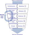 |
Fig. C.2 Visualization illustrating the modular code structure of MoCSI. There are currently five module insertion points in the code, where users can insert modules to do calculations, change and insert physical parameters, or access and alter simulation parameters. Right after the simulation has been initialized (1), at the start of each iteration within a time step (2), after the update of the temperature within the iterations of a time step (3), after the time step has converged (4), and during the post-processing of the simulation (5). If there are no temperature-dependent parameters and no iteration is necessary, insertion points three and four are equivalent. Each module instance represents its own unique set of modules which can be freely selected by the user. |
Appendix D Influence of temperature dependence
The application of MoCSI to the Kolobok crater has been performed with constant thermal parameters. This allowed a comparison to the results of Okada et al. (2020), but neglects any influence of temperature to these parameters. Especially for the thermal conductivity, this influence can be orders of magnitude, when assuming granular or a highly porous material (Hayne et al. 2017; Gundlach & Blum 2013). While a full investigation into the parameter space of temperature-dependent thermal conductivity and specific heat capacity is beyond the scope of this paper, we do want to offer a consideration of its influence on the presented results.
The Gundlach & Blum (2013) thermal conductivity model is readily available in MoCSI and incorporates also the conductance through a radiation term in large pores. We note that the Gundlach & Blum (2013) model describes regolith, which is not representative for the boulder-covered surface of Ryugu (Morota et al. 2020). Therefore it is not an appropriate choice for describing Ryugu’s surface itself; however using it for an inter-model comparison between temperature-dependent and non-temperature-dependent parameters remains suitable. The parameters used for the thermal conductivity model are given in Table D.1.
To approximate the temperature dependency of the thermal parameters on Ryugu, we chose to use measurements of these parameters performed on meteorites. The closest meteoritic analogue to Ryugu would be CI-meteorites (Yokoyama et al. 2023), but no complete data on both thermal conductivity and specific heat capacity could be acquired. Instead we chose CM2-type data measured from the Cold Bokkeveld meteorite by Opeil et al. (2020). The resulting temperature-dependent values are depicted in Fig. D.1. The specific heat capacity value had to be capped, as the measurements have only been performed up to 300 K and extrapolating the fit function beyond about 320 K yields unrealistic values. This was not necessary for the thermal conductivity, as beyond 300 K the value is dominated by the radiative term. The black dashed lines in the figure represent the constant values, that were used as a comparison case.
The simulation configuration chosen was the same as in Sect. 4, where a full orbit has been simulated to equilibrate the temperature profile, before simulating a single day at high temporal resolution. We compare the results for both the temperature-dependent and non-temperature-dependent case in Fig. D.2 evaluating them at the same times as in Sect. 4. A good agreement is seen for noon and close to noon times, when temperatures are around (±15 K) the values of the constant simulation. Even on the sunrise flank of the profile, where temperatures are around 300 K, the differences are less than 10 K. Only during night, when the thermal inertia exerts the strongest influence on the temperature profile, can large differences be seen > 20 K.
We conclude that the influence on the results that were discussed in Sect. 4 are small for most values, since TIR measurements are performed on the day-side of Ryugu. The influence of the temperature-dependence can shift the temperatures, but it is likely only be a small contribution to the differences seen between models and measurements. For the discussion of cooling curves, especially during the night-time however, temperature-dependence can play a major role, when the diurnal temperature is sufficiently large.
Parameters used for the Gundlach & Blum (2013) thermal conductivity model.
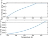 |
Fig. D.1 Temperature dependency of the thermal conductivity and specific heat capacity used for the comparison between temperature-dependent and non-temperature-dependent case. The black dashed line marks the value used for the non-temperature-dependent case. |
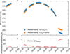 |
Fig. D.2 Comparison of median temperatures between a temperature-dependent thermal parameter case in the blue dots and a non-temperaturedependent thermal parameter case in the orange squares. The absolute median temperature differences are shown below. |
All Tables
Physical parameters used in the validation of MoCSI and comparison to 1DTM and heat1D.
All Figures
|
Fig. 1 Example of possible FEM grid in one dimension consisting of five nodes at positions xi, with areas Ai making up four linear elements of length, lm. The length between elements and the area at the position of the nodes do not have to be uniform. |
| In the text | |
|
Fig. 2 Visualization of core-code capabilities and standard time-stepping loop of MoCSI. Optionally executed functionality is marked as (opt.). The core code mainly provides utilities needed for the simulations. It loads shape models, generates the grid from user specifications, loads and creates snapshots as restoration points, and provides infrastructure such as matrices and solvers for linear systems of equations. The time-stepping loop is shown in detail. It consists of the outer time-integration loop and an inner iteration loop, which is used when nonlinear terms are present within the equations. If active, the steps marked in red are executed, and a check of the change in temperature against a user-specifiable abort criterion, ε, is done after every inner iteration; if the difference is larger than this criterion, it is redone, but with the modules in the pre-time step having access to the previously calculated temperatures. |
| In the text | |
|
Fig. 3 Temperature profiles comparing results of MoCSI code with an analytical solution given by Eq. (18), and residuals between both solutions. The MoCSI results were produced for a spatial resolution of 5 ∙ 10−5 m and a temporal resolution of 10−4 s after 1 s of simulation time. |
| In the text | |
|
Fig. 4 Convergence analysis of MoCSI code for the comparison against the analytical solution given by Eq. (18). Panel a: spatial convergence shown by plotting L2 error against element length. Panel b: temporal convergence shown by plotting L2 error against time-step length. Power-law fits for both plots have been produced, verifying that both the temporal and spatial convergence show the expected slopes of 1 and 2, respectively. |
| In the text | |
|
Fig. 5 Selected temperature profiles showing comparison between MoCSI code and 1DTM code at different times; i.e., the first time step after sunrise (panel a), the time step closest to noon (panel b), the first time step after sunset (panel c), and the time step closest to midnight (panel d). The differences during sunrise and sunset can be explained by the difference in surface-temperature prediction scheme, as also discussed in Schörghofer & Khatiwala (2024). Away from the boundary, where gradients are less steep, the two implementations show good agreement. Since surface temperatures differ slightly between the models, these differences propagate downward with the thermal profile. This explains the wavy structure in the residuals. |
| In the text | |
|
Fig. 6 Temperature profiles comparing results of MoCSI code with heat1d results and residuals between both models. An explanation for the differences between the models is given in Fig. 7. |
| In the text | |
|
Fig. 7 Temperature differences between standard heat1d implementation of surface-temperature calculation and two other implementations. The implementation represented by the blue line uses the temperatures of the next time step to approximate the temperature differential in the boundary condition. The implementation represented by the dashed orange line also uses the temperatures of the next time step and also calculates the heat conductivity at the interface between two grid points instead of directly at the points. While this is only a rough approximation of the changes a fully iterative heat1d would produce, it shows the general difference in temperatures we can expect from the changes to be in the low-Kelvin range. |
| In the text | |
|
Fig. 8 Visualization of energy transfer between two facets described through radiosity equations. Light from a given source directly illuminates one facet, which scatters the light to other topography that in return can scatter this light again. Furthermore, both facets have an associated temperature and thermal emission of infrared radiation, which they can transfer between each other. These three types of fluxes are represented within the radiosity equations. |
| In the text | |
|
Fig. 9 Top-down view of three-dimensional model of spherical crater with 14 198 facets, partially lit by the sun at a 15° incidence angle. Panel a: simulated surface temperatures. Panel b: differences between the analytical solution in Eq. (22) and simulated temperatures. While the residuals in the shadowed region reach up to ≲1 K, on the sunlit side they are around ≲0.1 K and below. |
| In the text | |
|
Fig. 10 Simulated temperatures and temperature differences between simulation and TIR measurements. Panel a: simulated surface temperatures within the Kolobok crater at 1 Aug 2018 18:16:30 UTC. Panel b: differences between measured and mapped TIR temperatures and the simulated temperatures. The TIR measurement was taken at 1 August 2018 18:16:32 UTC. The dark gray regions of Ryugu were not simulated. The absolute median difference between the TIR temperature and the simulated temperature is 16 K, with the simulated temperatures being hotter. |
| In the text | |
|
Fig. 11 Median temperature differences between the TIR temperatures and the simulated temperatures of all facets in the Kolobok crater for the global temperature mapping done for 1 August 2018 (all times UTC; Okada et al. 2020). The error bars indicate the range of the 10th and 90th percentiles of temperature differences on the 907 facets used for the simulation. The bottom panel shows the median incidence angle of all facets visible to TIR at the given time. A gap in the data between 10:30 and 14:00 exists and only points are used where more than 453 facets of the employed shape model were seen by TIR, which widens the data gap up to 17:00. |
| In the text | |
|
Fig. B.1 Selected temperature profiles showing the comparison between the MoCSI code and the 1DTM code. One row shows the two time steps that are between the ones shown in Fig. 5 in progressing time. |
| In the text | |
|
Fig. C.1 Illustration of the module pipeline workflow. Managing modules control their field parameter and pass it directly to the simulation environment, while sub-modules handle the actual computation. The number of sub-module layers depends on the complexity of the computation. For a more detailed explanation, see Sect. 2.3. |
| In the text | |
|
Fig. C.2 Visualization illustrating the modular code structure of MoCSI. There are currently five module insertion points in the code, where users can insert modules to do calculations, change and insert physical parameters, or access and alter simulation parameters. Right after the simulation has been initialized (1), at the start of each iteration within a time step (2), after the update of the temperature within the iterations of a time step (3), after the time step has converged (4), and during the post-processing of the simulation (5). If there are no temperature-dependent parameters and no iteration is necessary, insertion points three and four are equivalent. Each module instance represents its own unique set of modules which can be freely selected by the user. |
| In the text | |
|
Fig. D.1 Temperature dependency of the thermal conductivity and specific heat capacity used for the comparison between temperature-dependent and non-temperature-dependent case. The black dashed line marks the value used for the non-temperature-dependent case. |
| In the text | |
|
Fig. D.2 Comparison of median temperatures between a temperature-dependent thermal parameter case in the blue dots and a non-temperaturedependent thermal parameter case in the orange squares. The absolute median temperature differences are shown below. |
| In the text | |
Current usage metrics show cumulative count of Article Views (full-text article views including HTML views, PDF and ePub downloads, according to the available data) and Abstracts Views on Vision4Press platform.
Data correspond to usage on the plateform after 2015. The current usage metrics is available 48-96 hours after online publication and is updated daily on week days.
Initial download of the metrics may take a while.