| Issue |
A&A
Volume 706, February 2026
|
|
|---|---|---|
| Article Number | A19 | |
| Number of page(s) | 13 | |
| Section | Astrophysical processes | |
| DOI | https://doi.org/10.1051/0004-6361/202557180 | |
| Published online | 27 January 2026 | |
Statistics of the projected angles between the black-hole spin and the host-galaxy rotation axes from NewHorizon
1
ILANCE, CNRS – University of Tokyo International Research Laboratory Kashiwa Chiba 277-8582, Japan
2
Kavli IPMU (WPI), UTIAS, The University of Tokyo Kashiwa Chiba 277-8583, Japan
3
Department of Physics, School of Science, The University of Tokyo 7-3-1 Hongo Bunkyo-ku Tokyo 113-0033, Japan
4
Research Institute, Kochi University of Technology Tosa Yamada Kochi 782-8502, Japan
5
Co-creation Organization of Regional Innovation, Kochi University of Technology Tosa Yamada Kochi 782-8502, Japan
6
Institut d’Astrophysique de Paris, CNRS and Sorbonne Université, UMR 7095 98 bis Boulevard Arago F-75014 Paris, France
7
Institute of Astronomy and Astrophysics, Academia Sinica, No. 1, Section 4 Roosevelt Road Taipei 10617, Taiwan
8
Department of Astronomy and Yonsei University Observatory, Yonsei University Seoul 03722, Republic of Korea
★ Corresponding author: This email address is being protected from spambots. You need JavaScript enabled to view it.
Received:
10
September
2025
Accepted:
4
December
2025
Abstract
Understanding the alignment between active galactic nucleus (AGN) jets and their host galaxies is crucial for interpreting AGN unification models, jet feedback processes, and the coevolution of galaxies and their central black holes (BHs). In this study, we use the high-resolution cosmological zoom-in simulation NEWHORIZON, which self-consistently evolves BH mass and spin, to statistically examine the relationship between AGN jet orientation and host galaxy structure. Building upon our previous work, we extend the analysis of projected (2D) alignment angles to facilitate more direct comparisons with recent observational studies. In our methodology, galaxy orientations are estimated using optical position angles derived from synthetic DESI-LS and Euclid images, while BH spin vectors serve as proxies for AGN jet directions. From a carefully selected sample of 100 BH–galaxy systems at low redshift, we generate a catalog of 5000 mock optical images using a Monte Carlo approach that samples random viewing angles and redshifts. Our results reveal a statistically significant tendency for AGN jets to align with the orientation of their host galaxies, consistent with recent observations combining very long baseline interferometry (VLBI) and optical imaging of nearby AGNs. Furthermore, we find a slightly stronger alignment when using kinematic position angles derived from synthetic MaNGA-like stellar velocity fields. These findings underscore the importance of combining morphological, kinematic, and polarimetric information to disentangle the complex interplay between BH spin evolution, accretion mode, and the galactic environment in shaping the direction of relativistic jets.
Key words: black hole physics / methods: numerical / galaxies: evolution / galaxies: general / galaxies: kinematics and dynamics / galaxies: stellar content
© The Authors 2026
 Open Access article, published by EDP Sciences, under the terms of the Creative Commons Attribution License (https://creativecommons.org/licenses/by/4.0), which permits unrestricted use, distribution, and reproduction in any medium, provided the original work is properly cited.
This article is published in open access under the Subscribe to Open model. This email address is being protected from spambots. You need JavaScript enabled to view it. to support open access publication.
1. Introduction
Most galaxies host supermassive black holes (BHs) in their central parts. While their origins remain unanswered yet, the coevolution of the BHs and their galaxies is supposed to be crucial in explaining the universality and diversity in present-day galaxies. Black holes grow by accreting mass from their host galaxies and generate relativistic jets that interact with both the interstellar and inter-galactic media. Those jets regulate the star formation activities in the host galaxy (e.g., Di Matteo et al. 2005; Springel et al. 2005; Schawinski et al. 2006; Croton et al. 2006; Sijacki et al. 2007; Booth & Schaye 2009; Dubois et al. 2012; Choi et al. 2015; Kurinchi-Vendhan et al. 2024). Therefore, in addition to their strong gravitational interaction, the BHs play significant roles in reshaping the gas, stellar, and dark matter distribution from the central to outer parts of their host galaxies (e.g., Peirani et al. 2008; Duffy et al. 2010; Martizzi et al. 2013; Dubois et al. 2016; Peirani et al. 2017, 2019; Ardila et al. 2021, and references therein).
A critical and intriguing aspect of this phenomenon is the alignment between BH jets and their host galaxies. Indeed, the orientation of a jet relative to a galaxy’s stellar disk or large-scale structure can provide important insights into the processes governing BH spin, accretion disk orientation, galaxy mergers, and the cosmic history of angular momentum transfer. So far, the observational results are rather diverse and do not offer a clear picture. The jet directions in elliptical galaxies and Seyfert hosts seem to be randomly distributed with respect to their host galaxies’ stellar or gas rotation axes (Kinney et al. 2000; Schmitt et al. 2002; Gallimore et al. 2006). On the other hand, several statistical analyses reported a correlation between the radio major axis and the optical minor axis in radio-quiet passive ellipticals (Battye & Browne 2009) or a preferential alignment between radio jet axes and the minor axis in some spiral galaxies and Seyfert 2 active galactic nuclei (AGNs; Saripalli & Subrahmanyan 2009).
More recently, high-resolution and statistically robust studies have sharpened the evidence of nonrandom jet–galaxy alignments. Zheng et al. (2024) examined a sample of over 3600 radio-loud AGNs and found population-level evidence of alignment between radio jet orientations and the minor axes of their host galaxies. These results lend strong support to models involving coherent accretion flows whereby gas inflow maintains a consistent direction over time. Complementing this, Fernández Gil et al. (2024), using very long baseline interferometry (VLBI) and optical imaging for a large sample of nearby AGNs, reported a statistically significant orthogonal alignment between parsec-scale radio jets and the major axes of their host galaxies. This highlights the strong interplay between supermassive BHs, their host galaxies, and their coevolution over cosmic time.
On larger cosmic scales, Jung et al. (2025) investigated the influence of the cosmic web on AGN orientation, finding a correlation between AGN jet directions and the filamentary structure of the large-scale environment, especially for central galaxies in nodes of the cosmic web (see also Hutsemékers et al. 2014). This implies that both local galactic dynamics and cosmological inflow patterns may shape BH spin axes and jet orientations. Together, these studies highlight a multi-scale origin for jet–galaxy alignment, in which internal disk-driven torques, secular evolution, and cosmic web anisotropies all play a role (see, for example, Laigle et al. 2015; Codis et al. 2018).
The statistical alignment between AGN jets and their host galaxies suggests a possible physical connection between the jet-launching mechanism and the angular momentum axis of the central BH. The observed diversity in alignment is underpinned by theoretical models that distinguish between different modes of BH fueling. In the chaotic accretion paradigm proposed by King & Pringle (2006), gas accretes onto the BH in small, randomly oriented episodes, leading to frequent spin reorientations, and thus random jet directions. This model explains the misalignment seen in elliptical galaxies and in many Seyferts with disrupted gas inflows. Moreover, Hopkins et al. (2012) also predicted a weak correlation between the nuclear axis and the large-scale disk axis, using high-resolution simulations of gas inflows from galaxy to parsec scales around AGNs. Alternatively, coherent accretion, in which gas flows maintain a consistent angular momentum axis over time, can align the BH spin with the galaxy disk. Dotti et al. (2013) showed that in gas-rich disk galaxies, sustained inflow can rapidly align the BH spin with the inner disk, particularly in the presence of massive circumnuclear structures. This alignment may be aided by relativistic disk warping and the Bardeen–Petterson effect (Bardeen & Petterson 1975), which causes the inner accretion disk to align with the BH spin axis due to Lense–Thirring precession. The timescale of this process is believed to be much shorter than the lifetime of outflows or jets (Natarajan & Pringle 1998), suggesting that jet directions are generally not determined by the BH spin.
Evidence from X-ray observations demonstrating the ability of AGN to suppress cooling in galaxy clusters (e.g., Bîrzan et al. 2004; McNamara et al. 2005; Wise et al. 2007) motivated the incorporation of BH feedback into galaxy-formation models. Early implementations first appeared in semi-analytic frameworks (Bower et al. 2006; Croton et al. 2006; Lagos et al. 2008) and shortly thereafter in pioneering hydrodynamical simulations (e.g., Di Matteo et al. 2005; Booth & Schaye 2009). Since then, AGN feedback has become a standard component of cosmological simulation suites.
A number of widely used large-scale simulations adopt a single, usually thermal, feedback channel associated with high Eddington ratios (the so-called “quasar” mode) such as in OWLS (Schaye et al. 2010), MAGNETICUM (Hirschmann et al. 2014), EAGLE (Schaye et al. 2015), MASSIVEBLACK-II (Khandai et al. 2015), ROMULUS (Tremmel et al. 2017), and ASTRID (Bird et al. 2022). Other projects have moved toward more complex, two-mode prescriptions that alter the feedback mechanism at low accretion rates. ILLUSTRISTNG, for instance, transitions to a kinetic wind model inspired by advection-dominated, inflow-outflow solution (ADIOS: Blandford & Begelman 1999) type outflows (Weinberger et al. 2017), while the original ILLUSTRIS simulation injected thermal bubbles to mimic jet-inflated lobes (Sijacki et al. 2007; Vogelsberger et al. 2014). Still others employ explicit kinetic jets (Horizon-AGN: Dubois et al. 2014a; NewHorizon: Dubois et al. 2021; SIMBA: Davé et al. 2019), in some cases supplemented by additional processes such as AGN-driven X-ray heating (e.g., in SIMBA).
Underlying these implementations is a growing effort to model the sub-resolution physics of BH growth and energy release more realistically. Recent developments include treatments of accretion-disk structure, angular-momentum transport, and BH spin evolution (e.g., Fanidakis et al. 2011; Dubois et al. 2012; Steinborn et al. 2015; Fiacconi et al. 2018; Griffin et al. 2019; Huško et al. 2022; Koudmani et al. 2024; Sala et al. 2024). An additional line of work explores the consequences of super-Eddington accretion, incorporating both its radiative and mechanical feedback channels, which has renewed relevance for understanding rapid early BH growth (Rennehan et al. 2024; Bennett et al. 2024; Huško et al. 2025a,b).
The relative orientations between the BH spin and galaxy rotation axes have been investigated using high-resolution cosmological simulations (Dubois et al. 2014b; Beckmann et al. 2024; Peirani et al. 2024). In particular, Peirani et al. (2024) suggested that signatures of jet–galaxy alignment could be detectable through observational measurements of the projected (2D) misalignment angles, but their analysis does not fully account for projection effects inherent in observational data. The present paper aims to revisit their work in the 2D analysis, to better bridge the gap between simulations and recent observational findings. This paper is structured as follows. Section 2 provides a brief overview of the NEWHORIZON simulation and describes the numerical methodology employed in this work. Section 3 presents the main results, including statistical trends for both intrinsic spin–position angle misalignments and projected jet–galaxy misalignment angles. Section 4 summarizes our findings and offers concluding remarks.
2. Methodology
Throughout this paper, we analyse the results of the NEWHORIZON1 simulation. The details of the simulation have been described in many previous papers (e.g, Dubois et al. 2021; Peirani et al. 2024), so we only summarize here its main features.
2.1. The NEWHORIZON simulation
NEWHORIZON is a high-resolution zoom-in simulation from the HORIZON-AGN simulation (Dubois et al. 2014a), focused on a spherical sub-volume with a radius of 10 comoving Mpc. A standard ΛCDM cosmology was adopted with the total matter density Ωm = 0.272, the dark energy density ΩΛ = 0.728, the baryon density Ωb = 0.045, the Hubble constant H0 = 70.4 km s−1 Mpc−1, the amplitude of the matter power spectrum σ8 = 0.81, and the power-law index of the primordial power spectrum ns = 0.967, according to the WMAP-7 data (Komatsu et al. 2011). The initial conditions were generated with MPGRAFIC (Prunet et al. 2008) at the resolution of 40963 for NEWHORIZON in contrast to 10243 for HORIZON-AGN. The dark matter mass resolution reaches 1.2 × 10⁶ M⊙ compared to 8 × 10⁷ M⊙ in HORIZON-AGN. As far as star particles are concerned, their typical mass resolution is ∼104 M⊙ for NEWHORIZON.
Both simulations were run with the RAMSES code (Teyssier 2002) in which the gas component is evolved using a second-order Godunov scheme and the approximate Harten-Lax-Van Leer-Contact (HLLC, Toro 1999) Riemann solver with linear interpolation of the cell-centered quantities at cell interfaces using a minmod total variation diminishing scheme. In NEWHORIZON, refinement is performed according to a quasi-Lagrangian scheme with approximately constant proper highest resolution of 34 pc. The refinement is triggered in a quasi-Lagrangian manner, if the number of DM particles becomes greater than 8, or the total baryonic mass reaches 8 times the initial DM mass resolution in a cell. Extra levels of refinement are successively added at z = 9, 4, 1.5 and 0.25 (i.e., for expansion factor a= 0.1, 0.2, 0.4, and 0.8, respectively). The simulation is currently completed down to redshift z = 0.18.
It is well established that adaptive mesh refinement (AMR) codes, such as RAMSES, do not conserve angular momentum exactly, particularly at refinement-level transitions. This limitation may affect simulations of rotationally supported systems. More generally, no numerical method (e.g., AMR, smoothed particle hydrodynamics, moving-mesh schemes) preserves angular momentum perfectly. Discretization effects, numerical viscosity, and sampling noise inevitably introduce small torques (Commerçon et al. 2008; Hopkins 2015). Nevertheless, the angular-momentum content of simulated galaxies depends on much more than strict numerical conservation. The development of hydrodynamic instabilities plays a central role, as do stellar and AGN feedback, the structure of the interstellar medium, and its turbulent properties (e.g., Sijacki et al. 2012). Despite these challenges, the galaxies formed in NewHorizon exhibit morphologies that are broadly realistic, particularly in the case of spiral galaxies, providing qualitative support for the modeling when compared to observed galactic structural properties. The relatively modest impact of numerical resolution on galaxy spin is also illustrated in Dubois et al. (2014c).
NEWHORIZON encompasses a wide range of sub-grid models such as gas cooling, UV background, a model of star formation whose efficiency depends on the local turbulent Mach number and virial parameter (Kimm et al. 2017; Trebitsch et al. 2017, 2021), a model of type II supernovae based on the amount of linear momentum injected at the adiabatic and snow-plow phase (Kimm & Cen 2014; Kimm et al. 2015) or a model for BH mass growth and AGN feedback in alternating radio/quasar (jet/heating) mode (Dubois et al. 2012) coupled to a model of BH spin evolution (Dubois et al. 2014b). For this aspect, the BH spin is modeled on-the-fly in NEWHORIZON and updated according to the gas accretion and BH-BH mergers. In the radio/jet mode, BHs power jets that continuously release mass, momentum and energy. Bipolar jets are assumed as a cylinder of size Δx in radius and semi-height, centered on the BH (Dubois et al. 2010). angle). The jets are launched with a speed of 104 km/s. Note that star formation and feedback in NEWHORIZON are based on small-scale physics, combining theoretical models with very high–resolution simulations (see Dubois et al. 2021, and references therein). Black hole and AGN physics, however, are mainly calibrated using the local MBH–M★ in lower-resolution (∼kiloparsec) simulations (Dubois et al. 2012).
It should be stressed that in our simulations, the gas accretion disk around the BH is not spatially resolved. To address this, we assumed that the angular momentum of the accretion disk aligns with that of the gas measured at a distance of 4Δx ∼ 136 pc (where Δx is the highest spatial resolution) from each BH. Although this scale is much larger than the true physical size of the accretion disk, it provides a reasonable approximation, under the expectation that the orientation of the angular momentum is largely preserved as gas flows inward. This assumption is supported by the high-resolution simulations of Maio et al. (2013), who found that the angular momentum orientation is conserved down to scales of 1 pc, even in the presence of strong star formation feedback. However, alternative perspectives exist in the literature. Levine et al. (2010) reported that on scales of ∼100 pc, the direction of angular momentum can differ significantly from that on kiloparsec scales between z = 4 and z = 3. This variation arises mainly from infalling gas clumps whose interactions with the disk can substantially alter the angular momentum of nuclear gas. Similarly, Hopkins et al. (2012) found only a weak correlation between the orientation of the nuclear axis and the larger-scale disk axis in high-resolution simulations of gas inflows from galaxy to parsec scales around AGN. Such sudden misalignments can result from massive clumps falling slightly off-axis or from gravitational instabilities. It is important to note that these studies focused on gas-rich galaxies at high redshift, where turbulent gas motions are likely to have a strong impact on angular momentum alignment.
Additionally, we analyzed two other zoom simulations (nicknamed GALACTICA) focusing on isolated galaxies. For them, we used exactly the same physics and mass resolution as NEWHORIZON but they are located in different regions of HORIZON-AGN (see, e.g., Park et al. 2021).
2.2. Galaxy and black hole catalogs
The galaxy-BH catalog was produced using the same methodology described in Peirani et al. (2024) or adopted in previous studies using either HORIZON-AGN or NEWHORIZON (e.g., Volonteri et al. 2016; Smethurst et al. 2024; Beckmann et al. 2024). At a given redshift, we linked the primary BH to their host galaxy by selecting the most massive BH to be contained within two half mass radii (hereafter R1/2) of the galaxy’s center, using an iterative loop. The other BHs contained within two half mass radii were labeled as “secondary” or “wandering” BHs and were discarded from our analysis. In this scheme, we used a shrinking sphere approach (Power et al. 2003) to determine precisely the galaxy center. The half-mass radius2 of each galaxy was estimated by taking the geometric mean of the half-mass radius of the projected stellar densities along each of the simulation’s Cartesian axes. Note that BHs with mass below 2 × 10⁴ M⊙ are discarded from the analysis because they are too close to the initial seed BH mass and likely to suffer from mass resolution.
Since NEWHORIZON is a zoom simulation, low-mass resolution dark matter particles might “pollute” some halos, especially when they are located close to the boundary of the high resolution area. We, however, allow the selection of BHs in “contaminated” DM halos if the low resolution DM particles represent less than 0.1% of the total mass of the halos.
We also only selected galaxies with a stellar mass3 greater than 108 M⊙ to be more consistent with galaxies selected in the MaNGA survey (Mapping Nearby Galaxies at Apache Point Observatory, Bundy et al. 2015). All these constraints lead to a sample of 100 galaxy-BH pairs. We checked that the different BHs are in radio mode. If a given BH is not in radio mode at the last snapshot (z = 0.18), we selected the closest snapshot (that is, at a slightly higher redshift) where this constraint is satisfied.
Figure 1 shows the variation in a primary BH’s mass against the host galaxy mass at a redshift of ∼0.18. As was previously noted by Dubois et al. (2021), central massive BHs in NEWHORIZON typically experience significant growth only in galaxies with stellar masses exceeding a few 1010 M⊙. In contrast, for galaxies with stellar masses below 5 × 10⁹ M⊙, BH growth is generally suppressed by supernova feedback (see also Dubois et al. 2015; Habouzit et al. 2017; Trebitsch et al. 2017; Lapiner et al. 2021). Additionally, because of their low initial (seed) masses, BHs in these low-mass systems (particularly dwarf galaxies) often struggle to remain anchored at the centers of their host galaxies, as highlighted by Beckmann et al. (2023). As a result, the majority of BHs in the simulation undergo minimal growth throughout its duration. Overall, across all stellar mass bins, the BHs in our sample are slightly less massive than in observations, lying up to one order of magnitude below the bulk of the observed BH masses (see, e.g., Fig. 22 of Dubois et al. 2021). Yet our model reproduces both the slope of the local BH mass-total stellar mass relation and the break that appears to be emerging from observational constraints (e.g., Reines & Volonteri 2015). In our framework, BH growth remains inefficient in dwarf galaxies, becomes more effective once the host reaches sufficient mass (∼3 × 10⁹ M⊙), and eventually enters an AGN self-regulated phase. This mass-dependent transition captures the key qualitative features implied by current observations and theoretical models of BH-galaxy coevolution.
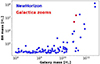 |
Fig. 1. Variations in the primary BH mass with respect to their host (stellar) galaxy mass at z ∼ 0.18. Our final catalog consists of 100 BHs all in radio mode, including BHs extracted from the two GALACTICA zooms. Overall, across all stellar mass bins, BHs in NEWHORIZON are under-massive in comparison to observations, lying up to one orders of magnitude below the bulk of the observed BH masses (see, e.g., Fig. 22 of Dubois et al. 2021). |
2.3. Synthetic DESI-LS and Euclid optical images
To facilitate a comparison with recent observational trends, particularly those reported by Zheng et al. (2024), Fernández Gil et al. (2024) and Jung et al. (2025), we produced a set of synthetic DESI-LS (Dey et al. 2019) r-band optical images. For this purpose, we employed the SUNSET code, a module included in the RAMSES package that generates realistic galaxy photometry, images, and spectra. Each stellar particle was assumed to behave as a single stellar population. We used here a Chabrier initial mass function (Chabrier 2003), and we adopted the stellar population synthesis model of Bruzual & Charlot (2003) to compute the contribution of each stellar particle to the mock image. Although the impact of dust attenuation is expected to be limited in the r band, the original version of the code was updated to incorporate dust effects. To this regard, the dust column density in front of each stellar particle was computed using the gas-phase metallicity as a proxy for the dust distribution. The contribution of all gas cells in front of a particle was accounted for, assuming that 40% of the mass of metals in gas cells are locked in dust grains, which is the fraction in the Milky-Way (see Dwek 1998) and in many other evolved galaxies (Rémy-Ruyer et al. 2014). To compute attenuation by dust, we adopted the value of the ratio of visual extinction to reddening RV = 3.1 for the Milky Way dust grain model presented by Weingartner & Draine (2001). While more advanced radiative transfer codes such as SKIRT (Camps & Baes 2015, 2020) are available for simulating photon propagation in astrophysical systems, SUNSET offers a practical compromise between physical realism and computational efficiency.
Following the methodology applied in Peirani et al. (2024) for analyzing projected 2D orientation angles, we used a Monte Carlo approach to generate the synthetic images. For each of the 100 galaxies in our sample, we used SUNSET to create 50 synthetic optical images by randomly assigning a redshift in the range 0.02 < z < 0.18 and a random spatial orientation. These mock images, generated by “observing” the original galaxy from different angles and redshifts, are diverse enough to be considered as statistically independent realizations. Each image was produced in the r-filter at DESI-LS resolution (0.262 arcsec per pixel) and convolved with a point-spread function (PSF) characterized by a full width at half maximum (FWHM) of 1.2 arcsec (Dey et al. 2019). No further corrections, such as seeing adjustments, image noise, and sky background, were applied.
In parallel, we generated a second set of mock observations using the specifications of the Euclid mission (Euclid Collaboration: Mellier et al. 2025): a resolution of 0.1 arcsec per pixel, the IE band (or RIZ band), and a PSF with a FWHM of 0.16 arcsec (Euclid Collaboration: McCracken et al. 2026). For consistency, we used the same set of galaxies, orientations, and redshift assignments as those employed for the synthetic DESI-LS images.
2.4. Synthetic MaNGA velocity fields
The MaNGA survey (Bundy et al. 2015) employs integral field units (IFUs) composed of fiber arrays arranged in a hexagonal pattern. There are five IFU configurations consisting of 19, 37, 61, 91, and 127 fibers, corresponding to diameters of 12.5″, 17.5″, 22.5″, 27.5″, and 32.5″, respectively (Drory et al. 2015). The galaxy sample is divided into two subsets: the Primary and Secondary samples, which are optimized to achieve spatial coverage out to 1.5 Re and 2.5 Re, respectively.
To generate synthetic stellar velocity fields comparable to MaNGA observations, we first assigned an IFU to each of the 5000 galaxies in our mock sample. For this, we estimated the effective radius of each galaxy using DESI-LS synthetic r-band images, assuming a fixed redshift of z = 0.037 (i.e., the median redshift of the MaNGA survey). The galaxies were then randomly divided into two groups that reproduce the observed proportions of the primary and secondary samples. Each galaxy was subsequently assigned a specific IFU configuration to ensure optimal spatial coverage.
Next, we began by computing the projected, light-weighted velocity fields in the r band at DESI-LS resolution, convolved with a PSF of FWHM = 1.5 arcsec as a simplified emulation of the typical atmospheric seeing at the telescope site (Yan et al. 2016; Bottrell & Hani 2022; Sarmiento et al. 2023). From these velocity maps, we calculated the mean velocity in each IFU fiber by averaging over all pixels located within the corresponding fiber aperture. The target galaxy was then “observed” through the assigned IFU using three dithering positions (see, e.g., Fig. 4 of Sarmiento et al. 2023). Finally, the fiber values were recombined and sampled onto a grid of 0.5 × 0.5 arcsec2 pixels. We followed here the same procedure as the one described in Law et al. (2016); namely, the contribution of a fiber, i, to a specific pixel, p, is given by
 (1)
(1)
where rp, i is the distance between the pixel “p” and the center of the fiber “i”, σ = 0.7″ (Law et al. 2016), and wT is a normalizing factor to keep the flux constant. For other sophisticated methods for generating MaNGA images from cosmological simulations, we refer the readers to Bottrell & Hani (2022), Nanni et al. (2022) and Sarmiento et al. (2023) as well as Barrientos Acevedo et al. (2023) for SAMI-like synthetic observations.
2.5. Measurement of ellipticity and effective radius
For each of the 5000 DESI-LS or Euclid synthetic optical images, the semimajor and semiminor axis lengths, ellipticity, and orientation angle, ϕ (angle between the semimajor axis and the x axis), were computed on the basis of the inertia tensor Iαβ of the 2D flux distribution:
 (2)
(2)
 (3)
(3)
 (4)
(4)
where L(i) and xα(i) are the flux and the projected position vector of the i-th pixel within a given enclosed flux or light region (specified by the value of N). That intertia tensor is then diagonalized and the square root of the eigenvalues give the relative size of the semimajor and minor axis. The orientation angle can be derived from the eigenvalue vectors and its expression is summarized in Eq. (4). Note that a similar methodology have been used in other theoretical studies using large cosmological simulations (see, e.g., Suto et al. 2017; Okabe et al. 2018; Lagos et al. 2018; Rodriguez-Gomez et al. 2019; de Araujo Ferreira et al. 2025).
In the following, the effective radius, Re, is defined as half the length of the semimajor axis of the ellipse that encloses half of the total flux in the optical image. In Fig. 2, we present the variation in the effective radius computed from the 5000 synthetic DESI-LS r-band images as a function of stellar mass. For qualitative comparison with observational trends, we also show the mean and dispersion of half-light radii derived from the DESI Early Data Release (DESI Collaboration 2024), selecting all galaxies within the redshift range 0.02 < z < 0.18.
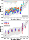 |
Fig. 2. Variations in the effective radius estimated from synthetic DESI-LS r-band images with respect to the galaxy mass (upper panel). For each galaxy, we generated 50 synthetic images by assigning random spatial orientations and redshifts in the range 0.02 < z < 0.18. For qualitative comparison with observational data, the black line represents the average half-light radius measured from the DESI Early Data Release (EDR), based on a sample of 151 530 galaxies within the same redshift range. The shaded gray area denotes the dispersion around the mean value. Overall, the trend observed in our synthetic sample agrees reasonably well with observational expectations, suggesting that the theoretical estimates of Re are reliable. In the lower panel, we compare the corresponding Re values derived from the synthetic Euclid images. On average, the effective radii estimated from the DESI-LS synthetic images are slightly larger than those obtained from Euclid, primarily due to the lower angular resolution of DESI-LS. |
Overall, the trend observed in our synthetic sample agrees reasonably well with observational expectations, suggesting that the theoretical estimates of Re are acceptable. However, we note a slight systematic excess in Re for low-mass galaxies (M★ < 109 M⊙) compared to observations. This discrepancy may arise from limitations in image resolution and/or the treatment of feedback processes in the simulation (Martin et al. 2025; Watkins et al. 2025).
In fact, the estimation of Re appears to be resolution-dependent. When the number of pixels covering a galaxy is reduced (such as at higher redshifts) the effective radius tends to be overestimated. This effect is illustrated in the lower panel of Fig. 2, where we compare the mean Re values obtained from DESI-LS and Euclid synthetic images. Although the filters and PSF convolution kernels differ between the two surveys, it is evident that the DESI-LS based estimates of Re are, on average, systematically larger than those derived from Euclid. This resolution bias is also noticeable in the upper panel of Fig. 2, suggesting that, for a particularly compact object, the estimated effective radius increases with redshift, corresponding to a decrease in pixel angular resolution.
2.6. Optical and kinematic position angle estimation
Throughout this work, position angles are defined with respect to the x axis (i.e., the horizontal axis) and range from 0° to 180°. We define the optical position angle (PAopt) for each DESI-LS and Euclid synthetic image as the angle between the semiminor axis of the projected ellipse (where the semimajor axis corresponds to the effective radius) and the x axis, following the methodology described in Sect. 2.5. We also compare trends measured at 2Re. Note that in the DESI Legacy Survey, the optical position angle, PAopt, is not measured explicitly at the effective radius but is inferred from a global model fit to the galaxy’s surface brightness profile. Since the fit is most constrained around the effective radius (where the signal-to-noise is good), the PA effectively reflects the orientation around Re.
To estimate the kinematic position angles, PAkin, from each synthetic MaNGA velocity field, we used the PAFIT package (Krajnović et al. 2006), a Python-based tool to determine the global kinematic position angle of galaxies (with 3σPAk values) and widely used in MaNGA observational analysis. The PAFIT routine basically performs a symmetry-based fitting of the observed velocity field and then tries different trial position angles and centers to find the configuration that minimizes the difference between the observed velocity field and the symmetrized model.
Following the definition in Franx et al. (1991), one can now estimate the misalignment angles ΔPAX − Y as the difference between the position angle PAX and the position angle PAY as
 (5)
(5)
In this parameterization, ΔPAX − Y lies between 0° and 90°. Moreover, ΔPAX − Y is not sensitive to differences of 180° between PAX and PAY.
To illustrate how accurately the optical and kinematic position angles trace the orientation of the “true” or intrinsic projected angular momentum of a galaxy, we present in Fig. 3 three representative examples from our sample. For each galaxy, we computed the misalignment angles, ΔPAgal − opt and ΔPAgal − kin, defined, respectively, as the angular differences between the projected galaxy spin, PAgal, and the optical (PAopt) or kinematic (PAkin) position angles. The first galaxy is an S0 with a passive evolutionary history. The second is a typical spiral galaxy, while the third is another S0 galaxy featuring a kinematically decoupled core (see, e.g., Peirani et al. 2025). The first column of Fig. 3 displays u–g–r composite images of these galaxies to provide a clear view of their projected morphological shapes. The second column shows the corresponding synthetic DESI-LS r-band images, convolved with an appropriate PSF. Each overlaid ellipse (solid line) encloses half of the galaxy’s total light. The semimajor axis of the ellipse defines the effective radius, while the orientation of the semiminor axis serves as a proxy for the direction of the projected stellar angular momentum. For comparison, these panels also include the projected BH spin vector (in black) and the projected stellar angular momentum vector (in cyan), the latter estimated from all stars within the half-mass radius (as defined above). The third column presents the light-weighted velocity fields at a high resolution. The fourth column shows the corresponding MaNGA-like velocity fields, along with the inferred kinematic position angle PAkin (dashed red line; see Sect. 2.4).
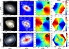 |
Fig. 3. Examples of synthetic optical and kinematic images derived in our analysis. Each row corresponds to a specific galaxy. The first column shows high resolution images using u-g-r bands, along with the value of the inclination angle (i) at which the galactic plan is viewed by the observer (see Fig. 19 in Peirani et al. 2024). The second column presents synthetic DESI-LS-like r-band images with a resolution of 0.262 arcsec per pixel, convolved with a PSF having a FWHM of 1.2 arcsec. The dashed black and red lines indicate the orientations of the major and minor photometric axes, respectively. The semimajor axis of each ellipse corresponds to the effective radius (Re), while the orientation of the semiminor axis serves as a proxy for the direction of the projected stellar angular momentum. For comparison, these panels also include the projected BH spin vector (in black) and the projected stellar angular momentum vector (in cyan), the latter estimated from all stars within the half-mass radius. In the second galaxy, the dotted line and the dotted ellipse indicate measurements at 2Re. The axis ratio q denotes the ratio of the semimajor to semiminor axes. In the third column, we show the corresponding high-resolution projected velocity fields, while the fourth column displays the synthetic MaNGA-like velocity fields. These latter were computed on a 0.5 × 0.5 arcsec per pixel grid, based on the interpolation of three dithering fiber configuration illustrated in the top-right corner of the third-column panels. Kinematic position angles (PAkin), derived using the PAFIT package (Krajnović et al. 2006), are indicated with dashed red lines. In the first example, both the optical and kinematic PAs closely trace the direction of the projected stellar spin. In the second example, the optical PA is less reliable due to the near-circular shape of the galaxy at one effective radius (q ≈ 1), while the kinematic PA more accurately captures the spin direction. The third example features a spheroidal galaxy with a kinematically decoupled core (a central stellar component rotating counter to the outer stellar population). This complex structure is not evident from the optical morphology alone, resulting in a more noticeable misalignment of ΔPAgal − opt = 15.2°. The kinematic estimate performs even worse, with ΔPAgal − kin = 22.4° and a substantial 3σPAk uncertainty of 28.2°, likely due to the presence of the decoupled core. |
In the first case (top row), the galaxy is an S0 with a passive evolutionary history and a relatively smooth light distribution, although some dust attenuation features are visible. The projected stellar angular momentum vector is nearly aligned with the semiminor axis, yielding a misalignment angle of ΔPAgal − opt = 0.3°. For the kinematic analysis, this galaxy is observed out to 1.5Re using a MaNGA IFU with seven fibers, due to its relatively compact size (Re = 1.97 kpc). The position angle determined from PAFIT fitting routine gives a misalignment of ΔPAgal − kin = 0.8° ±6.2°, also indicating a very good agreement with the projected galaxy spin direction.
In the second case, the ratio of the semimajor to semiminor axis measured at Re is close to unity (q = 1.05). As a result, the orientation of the semiminor axis becomes less reliable for estimating the direction of the true projected stellar angular momentum. In this configuration, we find a misalignment of ΔPAgal − opt = 11.0° which is still low. However, the accuracy improves significantly when the position angle is measured at 2Re (that is, ΔPAgal − opt = 0.9°, where q = 1.16). In contrast, the velocity field exhibits the typical signature of a spiral galaxy with strong rotational support. The synthetic MaNGA velocity map yields a kinematic misalignment of ΔPAgal − kin = 0.9°, with a high degree of confidence (3σPAk uncertainty of 1.2°).
The third case features an atypical spheroidal galaxy with a kinematically decoupled core, corresponding to a central stellar population that rotates in the opposite direction to the outer stellar component, a feature clearly visible in the synthetic velocity field. In this particular case, the main galaxy has undergone a merger with another (satellite) galaxy, with a mass ratio of 1:4. The stellar population that originally belonged to the satellite galaxy is now found at larger radii following the merger event and exhibits a counter-rotation with respect to the main stellar component. The gas accreted from the satellite galaxy has completely replaced the original gas of the host and also counter-rotates relative to the main stellar component. Consequently, as indicated by the stellar velocity field (third row, right panel), the BH spin, which aligns with the orientation of the accreted gas, follows the angular momentum of the outer stellar population rather than that of the central, decoupled core, which might have been expected initially. For more details on the formation of this particular galaxy, as well as a broader theoretical framework on the origin of counter-rotating galaxies, we refer the reader to galaxy G-31 in Peirani et al. (2025), and to Peirani et al. (2024) for the consequences on the evolution of its central BH, BH-549. In this example, the optical morphology alone does not reveal the presence of such a complex kinematic structure. However, the alignment is less evident, with a value of ΔPAgal − opt = 15.2°. The kinematic prediction performs even worse, with ΔPAgal − kin = 22.4° and a large 3σPAk uncertainty of 28.2°, likely due to the presence of the decoupled core. Note that, interestingly, the synthetic MaNGA image derived for this galaxy looks quite similar to the stellar MaNGA velocicy field derived from the galaxy PGC 66551 and studied in Katkov et al. (2024).
3. Results
3.1. Galaxy spin–position angle misalignment
The first step of our analysis was to assess the reliability of optical and kinematic position angles in tracing the orientation of a galaxy’s projected angular momentum. For consistency, we adopted the same definition of galaxy angular momentum as in our previous studies (Peirani et al. 2024, 2025), which was computed using all star particles located within the half-mass radius (as defined in Sect. 2.2).
In Fig. 4, we show the distributions of ΔPAgal − opt, derived from our catalogs of 5000 synthetic DESI-LS and Euclid optical images, and ΔPAgal − kin, derived from (5000) MaNGA-like synthetic velocity fields. For comparison, the optical PAs are measured at both one Re (top row) and two Re (bottom row).
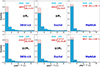 |
Fig. 4. Distributions of ΔPAgal − opt and ΔPAgal − kin. This figure presents the distributions of ΔPAgal − opt, the 2D misalignment angle between the projected stellar angular momentum vector of the galaxy and the optical position angle, defined as the orientation of the minor axis of the projected light ellipse. The first and second columns correspond to synthetic DESI-LS and Euclid images, respectively, with optical PAs estimated at one effective radius (top row) and at two effective radii (middle row). The third column shows the distributions of ΔPAgal − kin, defined as the angle between the projected spin vector of the galaxy and the kinematic PA derived from synthetic MaNGA-like stellar velocity fields. In all panels, hatched red histograms indicate results when only good cases (i.e., more reliable PA measurements) are selected. We also specify the number of “sources” or images used to derive the different histograms. |
Following the methodology adopted in Zheng et al. (2024) and Fernández Gil et al. (2024), we also analyzed trends using only “good cases” (that is, galaxies with more reliable PA estimates). In our analysis, good cases for optical images are defined as those with a projected axis ratio q > 1.2 and a ratio of Re (or 2Re) to the instrument’s pixel resolution greater than 5. For instance, this corresponds to Re > 1.13″ or Re > 0.66″ for DESI-LS, depending on whether the PA is measured at one or two effective radii. For the kinematic maps, good cases are deemed to be those that have PA uncertainties (3σPAk) that are less than 10° or 20°, respectively. These thresholds were chosen to roughly match the number of good cases of DESI-LS optical images for each Re-based measurement.
Figure 4 suggests that the kinematic PAs are a more accurate estimator for the “true” projected galaxy angular momentum. Approximately 80% of galaxies exhibit ΔPAgal − kin < 10° while 60% meet this threshold for the optical PAs. If we focus on the good cases, however, the three estimators perform almost equally well as 88.4%, 88.0%, and 94.4% of the DESI-LS, Euclid, and MaNGA subsamples, respectively, show ΔPA < 20°.
We also find that estimating optical PAs at 2Re slightly improves the overall alignment with the projected galaxy spin PAgal compared to measurements taken at Re, particularly for ΔPA < 10°. While the overall trends remain similar to those obtained using PAs measured at one effective radius, the differences between the three approaches become less pronounced when focusing on good cases. This suggests that, in well-resolved galaxies with reliable PA estimates, the dominant “noise” source in estimating the true misalignment is likely due to projection effects rather than instrumental limitations such as point spread function width or filter selection. Additionally, we observe no significant change in the distribution of ΔPAgal − kin when applying a more stringent selection criterion of 3σPAk < 10°, further supporting the robustness of the kinematic alignment trends.
We did not find a significant improvement in alignment statistics when switching from DESI-LS to Euclid, despite the latter’s higher resolution. One possible explanation is that the simulated galaxies studied in this work are in general well-resolved galaxies, even in DESI-LS. Euclid’s larger sample size will, however, allow this study to be extended to higher-redshift/lower-mass galaxies and will likely enable more precise conclusions in the future.
Our findings are consistent with previous studies. First, the distributions of optical position angles shown in Fig. 4 are similar to those obtained for elliptical galaxies from the EAGLE simulation (Fernández Gil et al. 2024), which also exhibit a high fraction of cases with ΔPA < 20°. Second, observational analyses generally report good agreement between optical and kinematic PAs. For example, based on a sample of approximately 2300 MaNGA galaxies, Graham et al. (2018) found a strong peak in the distribution for ΔPAopt − kin < 30° (see their Fig. 12). Specifically, they reported that 83.7% of regular early-type galaxies (ETGs) and 84.5% of spiral galaxies are aligned within ΔPAopt − kin < 10°, in good agreement with Krajnović et al. (2011), who found that 90% of 260 ETGs from the ATLAS3D survey lie within ΔPAopt − kin < 15°. Additionally, Barrera-Ballesteros et al. (2015) found that the morpho-kinematic misalignment is less than 22° in 90% of a sample of 103 interacting galaxies from the CALIFA survey (see their Fig. 4). In our case, the alignment trend is slightly weaker: as is shown in Fig. 5, we find that 72.8% and 82.4% of the sample exhibit optical–kinematic misalignment below 10° and 20°, respectively.
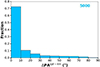 |
Fig. 5. Histogram of ΔPAopt − kin, the angles between optical and kinematic PAs derived from our sample of 5000 synthetic DESI-LS r-band and MaNGA velocity fields. 72.8% and 82.4% of the sample have optical-kinematic misalignment lower than 10° and 20°, respectively. Optical PAs are estimated at two effective radii. |
3.2. BH spin and jet versus PA misalignment
We now turn to the core objective of this study: investigating the degree of misalignment between AGN jets and the orientation of their host galaxies. Although the NEWHORIZON simulation does include AGN radio-mode feedback, clearly identifying jet structures in mock images remains challenging due to resolution limitations and the complexity of radio jet morphology. Instead, since AGN jets are launched along the direction of the BH spin in the simulation, we use the BH spin vector as a proxy for jet orientation. We note, however, that jets are intermittent phenomena and therefore not always observable, contrary to what is implicitly assumed in our approach. Incorporating a duty cycle for jet production and observability into our Monte Carlo framework is beyond the scope of the present paper, but should certainly be explored in future work to assess its potential impact. We also recall that all BHs in our sample are selected in the radio mode, which increases the likelihood of jet formation and thus partly alleviates concerns regarding duty-cycle realism.
It is important to acknowledge that AGN jets are not always perfectly aligned with the BH spin vector. As jets propagate from the accretion disk to galactic scales, their direction can be influenced by a number of factors: interaction with the multiphase interstellar medium (e.g., Mukherjee et al. 2018; Cielo et al. 2018; Junor et al. 1999; Borodina et al. 2025), jet precession (Dunn et al. 2006; Krause et al. 2019; Ubertosi et al. 2024), or motion through the intracluster medium (e.g., Heinz et al. 2006; Morsony et al. 2010, 2013; O’Dea & Baum 2023, and references therein). This potential issue might be partly alleviated in recent observational analyses (Fernández Gil et al. 2024; Zheng et al. 2024; Jung et al. 2025) by using VLBI to see the immediate surrounding of the BHs.
Moreover, as is discussed in Sect. 2, we stress again that the gas accretion disk around the BH is not spatially resolved in our simulations. we indeed assumed that the angular momentum of the accretion disk aligns with that of the gas measured at a distance of ∼136 pc (i.e., four times the highest spatial resolution) from each BH. This approximation could become problematic in cases where the nuclear axis is misaligned with the larger-scale disk axis, as was suggested by the high-resolution simulations of Hopkins et al. (2012).
Therefore, to account for potential misalignments between the nuclear axis and the large-scale galactic axis, as well as uncertainties related to jet propagation and projection effects, we introduced an artificial angular scatter to the 3D BH spin orientations. Specifically, we applied a uniform random perturbation between 0° and 30° to mimic misalignments that may arise during gas accretion episodes and/or as the jet interacts with the multiphase ISM during its propagation to larger scales. Larger scatter amplitudes would progressively dilute any intrinsic alignment signal, eventually driving the distribution toward a uniform one and making any physical correlation much more difficult to detect. Conversely, smaller scatter values preserve tighter alignment signatures, but may underestimate the true level of physical and observational uncertainties. Our adopted range therefore represents a conservative compromise for exploring how such uncertainties affect the predicted misalignment distributions. The jet position angle is then determined by projecting this perturbed spin vector in 2D, using the orientation of the host galaxy.
Figure 6 shows the distribution of ΔPAjet − opt, the angle between the projected jet direction and the optical PA, the latter derived from both DESI-LS and Euclid synthetic images4. For clarity, we present results only for the good cases and consider three models: one with no added scatter, and two with uniform scatter of up to 15° and 30°, respectively, applied to the 3D BH spin vectors. Trends for disk-dominated galaxies and spheroid-dominated galaxies are shown in the second and third columns, respectively. To simplify the analysis, and rather than following a more observationally consistent approach, we classified galaxies using the ratio of stellar rotational velocity (V*) to velocity dispersion (σ*), derived from the simulations. We adopted V*/σ* > 1.0 for disk-dominated systems and V*/σ* < 0.7 for spheroid-dominated systems (values commonly used in previous studies, e.g., Dubois et al. 2016; Peirani et al. 2017) We also computed ΔPAjet − kin, the misalignment between jets and the kinematic PA derived from synthetic MaNGA-like velocity fields. Note that, for optical images, we only report results using PAs measured at 2Re, as trends at Re are similar.
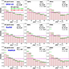 |
Fig. 6. Histograms of ΔPAjet − opt, the 2D misalignment angle between the projected galaxy spin and the optical position angle, derived from synthetic images from the DESI-LS (top row) and Euclid (middle row) catalogs, with measurements estimated at 2Re. The third row presents histograms of ΔPAjet − kin, the misalignment between the projected galaxy spin and the kinematic PA derived from synthetic MaNGA velocity fields. The first column includes results for the treatment of all good cases, defined by expected more reliable optical or kinematic PA measurements, while the second and third columns display trends for spheroid-dominated galaxies (V*/σ* < 0.7) and disk-dominated galaxies (V*/σ* > 1.0), respectively. In each panel, the black, green, and red hashed histograms represent the results with no added scatter, and with uniform scatter of up to 15° and 30° respectively, applied to the 3D BH spin vectors. The dashed magenta line refers to the uniform distribution and the number indicate the number of images used to derive the histrograms. Overall, a clear trend of alignment between the jet direction and the galaxy orientation is observed, with a higher fraction of galaxies exhibiting misalignment angles below 20°, even when random angular scatter is introduced to the BH spin. |
Our results indicate a statistically significant alignment trend even after taking account of realistic observational errors. Indeed, a large fraction of galaxies display ΔPA < 20°, consistent with a physical alignment between jets and galaxy orientation. A modest perturbation of 15° already reduces the strength of the signal, shifting the ΔPAjet − opt distribution closer to uniformity, although a clear excess of aligned systems remains. When the scatter is increased to 30°, the dilution becomes more pronounced, as was expected, yet the residual alignment persists at a statistically significant level. This systematic weakening of the signal with increasing perturbation amplitudes highlights both the robustness of the underlying alignment and the sensitivity of projected ΔPAjet − opt measurements to small-scale physical processes that can alter jet propagation. This confirms the findings of Peirani et al. (2024), where projected BH spin vectors were shown to align with the intrinsic galaxy spin.
Interestingly, we do not observe a strong difference in alignment trends between spheroidal (elliptical) and disk-dominated (spiral) galaxies. This is somewhat surprising as spiral galaxies typically assemble via secular internal evolution (e.g., Kormendy & Kennicutt 2004) and the steady accretion of cold gas along cosmic filaments (e.g., Kereš et al. 2005; Dekel & Birnboim 2006; Dekel et al. 2009; Danovich et al. 2015), whereas elliptical galaxies form mainly through major or repeated minor mergers that transform rotationally supported disks into pressure-supported spheroids (e.g., White 1978; Barnes 1992; Hernquist 1992; Naab et al. 2007; Bournaud et al. 2011; Rodriguez-Gomez et al. 2016). These differing evolutionary paths are thus expected to influence the orientation and stability of the central BH’s spin axis.
Here also, the distributions from DESI-LS and Euclid mock images are similar, despite Euclid’s superior spatial resolution. However, Euclid’s broader sky coverage and deeper imaging are expected to improve sample statistics in future analyses. Also, both optical and kinematic PAs yield comparable alignment trends, though the kinematic measurements show a slightly stronger alignment signal.
We also performed a Kolmogórov–Smirnov (KS) test for each distribution of Fig. 6 and analyzed the corresponding pKS values, which offer a binning-independent assessment of the distribution shape. The KS test is a non-parametric statistical method used to evaluate the goodness of fit between an empirical distribution and a reference distribution. In our case, we compare the observed distributions against a uniform distribution. In all cases presented in Fig. 6, the resulting pKS values tend toward zero, indicating that the observed distributions significantly deviate from uniformity.
Our findings agree well with recent VLBI-based observational studies. In particular, Fernández Gil et al. (2024) presented histograms of jet–galaxy PA differences using VLBI jets cross-matched with DESI Legacy Survey data (see their Fig. 3), showing similar alignment tendencies. Jung et al. (2025) reported that 39.8% in the “extended jet” sample have jets aligned within 30°. Our results show slightly higher alignment rates: 43.0%, 44.4%, and 42.0% for all, elliptical, and disk-dominated galaxies, respectively (DESI-LS, good cases), and 47.3% for the MaNGA-based analysis.
Zheng et al. (2024) also studied radio–optical PA misalignments using data from LOFAR (LoTSS DR2), FIRST, DESI Legacy Surveys, and SDSS. They found a prominent minor-axis alignment trend for radio AGNs, possibly more pronounced than in our results. This could be due to their focus on more massive systems, where jet alignment may be more tightly correlated with host galaxy structure.
To conclude, we examined the impact of galaxy stellar mass on the distribution of jet–galaxy misalignment angles. As is shown in Peirani et al. (2024), BHs residing in low-mass galaxies generally exhibit spins that are less well aligned with the angular momentum of their host galaxies compared to those in high-mass systems. This trend arises from the fact that, as is discussed in Sect. 2.2, BHs in low-mass galaxies are often off-centered and experience limited growth due to inefficient gas accretion. The results are presented in Fig. 7, where we distinguish between galaxies with stellar masses below 109 M⊙ and those above 1010 M⊙. Note that we did not include intermediate-mass galaxies (between 109 M⊙ and 1010 M⊙) to emphasize the contrast between the low- and high-mass regime trends. Also, for clarity, we show only the good cases and assume a uniform perturbation of 30° applied to the BH spin vectors. No morphological classification (e.g., disk or spheroid) is made in this analysis. Our findings reveal that, in low-mass galaxies, the distribution of jet–galaxy misalignment angles approaches a uniform distribution, indicating a lack of preferred orientation. This contributes to a dilution of the overall alignment signal when considering the full galaxy population. In contrast, high-mass galaxies tend to preserve a stronger alignment between the jet direction and galaxy orientation. It is worth noting that our high-mass sample is largely represented by Milky Way–mass galaxies. None of the brightest cluster galaxies (BCGs), for which the misalignment is expected to increase again (Dubois et al. 2014b; Bustamante & Springel 2019), are included in our sample.
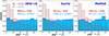 |
Fig. 7. Same as Fig. 6, but here we distinguish between galaxies with stellar masses below 109 M⊙ and above 1010 M⊙. The numbers indicated in each panel correspond to the sample sizes used to generate the histograms. Values in parentheses denote the KS test pKS values. The results suggest that low-mass galaxies exhibit a more uniform distribution of BH–galaxy misalignment angles (characterized by pKS > 0.05). Note that only good cases are shown, assuming a uniform perturbation of the BH spin of 30°, with no morphological distinction between spheroidal and disk galaxies. |
Finally, Fig. 7 indicates a transition at stellar masses between between 109 M⊙ and 1010 M⊙, marking a shift from chaotic to rotationally supported galaxies. It is interesting to note that this finding is in line with recent simulations that report a morphological transition occurring at a similar mass scale (e.g., Stern et al. 2021; Yu et al. 2021, 2023; Hafen et al. 2022; Gurvich et al. 2023; Hopkins et al. 2023; Benavides et al. 2025).
4. Summary and conclusions
The orientation of an AGN jet is a crucial probe of the interplay between BH spin, accretion physics, and the host galaxy structure. Whether the BH spin and/or the AGN jet are aligned with the angular momentum of the host galaxy’s stellar or gaseous disk remains an open question that holds implications for galaxy formation, BH coevolution, and feedback processes. Using the NEWHORIZON simulation, we performed a statistical analysis of the projected angles between the BH spin and the host galaxy rotation axes. In order to make a testable prediction for photometric and/or spectroscopic surveys of galaxies, we created mock catalogs of synthetics DESI-LS and Euclid optical images (r band) and synthetic MaNGA-like velocity maps for 100 simulated BH-galaxy systems viewed from 50 random line-of-sight directions. Then, we computed the optical and kinematic positions angles derived from the photometric images and velocity maps, respectively. Assuming that the BH spin axis is a good proxy of the observable AGN jet direction, we statistically examined the projected angles between the the BH spin direction and the host galaxy position angles. Our major findings are summarized as follows:
1. Both optical and kinematic position angles can be used as statistically reliable estimators for the projected orientation of the angular momentum axis of galaxies. For those systems with accurate morphological or kinematic measurements, approximately 90% and 95% of galaxies exhibit ΔPAgal − opt < 20° and ΔPAgal − kin < 20°, respectively.
2. Even after taking account of the possible misalignment of the BH spin and the jet directions, we found that the projected AGN jets and the position angles of their host galaxies exhibit a statistically significant alignment trend. These findings are in good agreement with recent observational studies that report similar alignment trends, including those by Zheng et al. (2024), Fernández Gil et al. (2024), and Jung et al. (2025), which use combinations of radio, optical, and spectroscopic data to probe jet-host alignment in nearby AGN systems.
3. Future analyses incorporating kinematic position angles from surveys such as MaNGA are very promising to test and refine the alignment trends identified in this work.
We note that kinematic position angles can be derived not only from the stellar component but also from the ionized gas, as measured by integral field unit surveys such as CALIFA or MaNGA. Including gas kinematics provide additional constraints on jet–galaxy misalignment, as gas may respond differently to AGN-driven outflows or environmental effects (see, e.g., Barrera-Ballesteros et al. 2015; Garay-Solis et al. 2023, 2024, 2025).
The potential dependence of jet–galaxy misalignment on the large-scale cosmic environment, such as proximity to cosmic filaments, has been explored in recent studies (e.g., Jung et al. 2025). However, investigating such environmental effects is beyond the scope of the present work. Our current analysis is indeed based on a relatively small sample of 100 BH–galaxy systems, which limits our ability to draw statistically robust conclusions about environmental trends. Nonetheless, this represents a promising avenue for future research. Expanding the sample size and incorporating environmental metrics could provide valuable insights into how cosmic structure influences the orientation and evolution of AGN jets relative to their host galaxies.
To conclude, the tendency for alignment between AGN jets and the spin axes of their host galaxies, suggested by both theoretical predictions and growing observational evidence, may have important implications for the coevolution of BHs and host galaxies, as well as models of galaxy formation in general. Future high-resolution radio surveys such as the ngVLA (the Next Generation Very Large Array, Murphy et al. 2018) or SKAO (Square Kilometre Array Observatory, Braun et al. 2019) combined with integral field spectroscopy, in particular MaNGA (Mapping Nearby Galaxies at Apache Point Observatory, Bundy et al. 2015) and MUSE (Multi Unit Spectroscopic Explorer, Bacon et al. 2010), will enable statistically robust, spatially resolved measurements of jet orientation and galaxy spin across cosmic time. On the theoretical side, future cosmological simulations that simultaneously resolve both large-scale environments and sub-parsec accretion physics, including magnetohydrodynamic and radiative feedback processes, will be crucial for understanding the origin and persistence of jet–galaxy alignment in different evolutionary contexts.
Acknowledgments
We warmly thank the referee for their insightful review and valuable comments. This research is partly supported by the JSPS KAKENHI grant Nos. 23H01212 (Y.S.). CL acknowledges the support of the French Agence Nationale de la Recherche (ANR), under grant ANR-22-CE31-0007 (project IMAGE). This work was granted access to the HPC resources of CINES under the allocations c2016047637, A0020407637 and A0070402192 by Genci, KSC-2017-G2-0003, KSC-2020-CRE-0055 and KSC-2020-CRE-0280 by KISTI, and as a “Grand Challenge” project granted by GENCI on the AMD Rome extension of the Joliot Curie supercomputer at TGCC. The large data transfer was supported by KREONET, which is managed and operated by KISTI. S.K.Y. acknowledges support from the Korean National Research Foundation (RS-2025-00514475; RS-2022-NR070872). This work was carried within the framework of the Horizon project (http://www.projet-horizon.fr). Most of the numerical modeling presented here was done on the Horizon cluster at Institut d’Astrophysique de Paris (IAP).
References
- Ardila, F., Huang, S., Leauthaud, A., et al. 2021, MNRAS, 500, 432 [Google Scholar]
- Aubert, D., Pichon, C., & Colombi, S. 2004, MNRAS, 352, 376 [Google Scholar]
- Bacon, R., Accardo, M., Adjali, L., et al. 2010, in Ground-based and Airborne Instrumentation for Astronomy III, eds. I. S. McLean, S. K. Ramsay, & H. Takami, SPIE Conf. Ser., 7735, 773508 [Google Scholar]
- Bardeen, J. M., & Petterson, J. A. 1975, ApJ, 195, L65 [Google Scholar]
- Barnes, J. E. 1992, ApJ, 393, 484 [NASA ADS] [CrossRef] [Google Scholar]
- Barrera-Ballesteros, J. K., García-Lorenzo, B., Falcón-Barroso, J., et al. 2015, A&A, 582, A21 [NASA ADS] [CrossRef] [EDP Sciences] [Google Scholar]
- Barrientos Acevedo, D., van der Wel, A., Baes, M., et al. 2023, MNRAS, 524, 907 [NASA ADS] [CrossRef] [Google Scholar]
- Battye, R. A., & Browne, I. W. A. 2009, MNRAS, 399, 1888 [CrossRef] [Google Scholar]
- Beckmann, R. S., Dubois, Y., Volonteri, M., et al. 2023, MNRAS, 523, 5610 [NASA ADS] [CrossRef] [Google Scholar]
- Beckmann, R. S., Smethurst, R. J., Simmons, B. D., et al. 2024, MNRAS, 527, 10867 [Google Scholar]
- Benavides, J. A., Sales, L. V., Wetzel, A., et al. 2025, MNRAS, submitted [arXiv:2508.00991] [Google Scholar]
- Bennett, J. S., Sijacki, D., Costa, T., Laporte, N., & Witten, C. 2024, MNRAS, 527, 1033 [Google Scholar]
- Bird, S., Ni, Y., Di Matteo, T., et al. 2022, MNRAS, 512, 3703 [NASA ADS] [CrossRef] [Google Scholar]
- Bîrzan, L., Rafferty, D. A., McNamara, B. R., Wise, M. W., & Nulsen, P. E. J. 2004, ApJ, 607, 800 [Google Scholar]
- Blandford, R. D., & Begelman, M. C. 1999, MNRAS, 303, L1 [NASA ADS] [CrossRef] [Google Scholar]
- Booth, C. M., & Schaye, J. 2009, MNRAS, 398, 53 [Google Scholar]
- Borodina, O., Ni, Y., Bennett, J. S., et al. 2025, ApJ, 981, 149 [Google Scholar]
- Bottrell, C., & Hani, M. H. 2022, MNRAS, 514, 2821 [NASA ADS] [CrossRef] [Google Scholar]
- Bournaud, F., Chapon, D., Teyssier, R., et al. 2011, ApJ, 730, 4 [NASA ADS] [CrossRef] [Google Scholar]
- Bower, R. G., Benson, A. J., Malbon, R., et al. 2006, MNRAS, 370, 645 [Google Scholar]
- Braun, R., Bonaldi, A., Bourke, T., Keane, E., & Wagg, J. 2019, arXiv e-prints [arXiv:1912.12699] [Google Scholar]
- Bruzual, G., & Charlot, S. 2003, MNRAS, 344, 1000 [NASA ADS] [CrossRef] [Google Scholar]
- Bundy, K., Bershady, M. A., Law, D. R., et al. 2015, ApJ, 798, 7 [Google Scholar]
- Bustamante, S., & Springel, V. 2019, MNRAS, 490, 4133 [CrossRef] [Google Scholar]
- Camps, P., & Baes, M. 2015, Astron. Comput., 9, 20 [Google Scholar]
- Camps, P., & Baes, M. 2020, Astron. Comput., 31, 100381 [NASA ADS] [CrossRef] [Google Scholar]
- Chabrier, G. 2003, PASP, 115, 763 [Google Scholar]
- Choi, E., Ostriker, J. P., Naab, T., Oser, L., & Moster, B. P. 2015, MNRAS, 449, 4105 [CrossRef] [Google Scholar]
- Cielo, S., Babul, A., Antonuccio-Delogu, V., Silk, J., & Volonteri, M. 2018, A&A, 617, A58 [CrossRef] [EDP Sciences] [Google Scholar]
- Codis, S., Jindal, A., Chisari, N. E., et al. 2018, MNRAS, 481, 4753 [Google Scholar]
- Commerçon, B., Hennebelle, P., Audit, E., Chabrier, G., & Teyssier, R. 2008, A&A, 482, 371 [NASA ADS] [CrossRef] [EDP Sciences] [Google Scholar]
- Croton, D. J., Springel, V., White, S. D. M., et al. 2006, MNRAS, 365, 11 [Google Scholar]
- Danovich, M., Dekel, A., Hahn, O., Ceverino, D., & Primack, J. 2015, MNRAS, 449, 2087 [Google Scholar]
- Davé, R., Anglés-Alcázar, D., Narayanan, D., et al. 2019, MNRAS, 486, 2827 [Google Scholar]
- de Araujo Ferreira, P., Napolitano, N. R., Casarini, L., et al. 2025, MNRAS, 539, 2855 [Google Scholar]
- Dekel, A., & Birnboim, Y. 2006, MNRAS, 368, 2 [NASA ADS] [CrossRef] [Google Scholar]
- Dekel, A., Sari, R., & Ceverino, D. 2009, ApJ, 703, 785 [Google Scholar]
- DESI Collaboration (Adame, A. G., et al.) 2024, AJ, 168, 58 [NASA ADS] [CrossRef] [Google Scholar]
- Dey, A., Schlegel, D. J., Lang, D., et al. 2019, AJ, 157, 168 [Google Scholar]
- Di Matteo, T., Springel, V., & Hernquist, L. 2005, Nature, 433, 604 [NASA ADS] [CrossRef] [Google Scholar]
- Dotti, M., Colpi, M., Pallini, S., Perego, A., & Volonteri, M. 2013, ApJ, 762, 68 [NASA ADS] [CrossRef] [Google Scholar]
- Drory, N., MacDonald, N., Bershady, M. A., et al. 2015, AJ, 149, 77 [CrossRef] [Google Scholar]
- Dubois, Y., Devriendt, J., Slyz, A., & Teyssier, R. 2010, MNRAS, 409, 985 [Google Scholar]
- Dubois, Y., Devriendt, J., Slyz, A., & Teyssier, R. 2012, MNRAS, 420, 2662 [Google Scholar]
- Dubois, Y., Pichon, C., Welker, C., et al. 2014a, MNRAS, 444, 1453 [Google Scholar]
- Dubois, Y., Volonteri, M., & Silk, J. 2014b, MNRAS, 440, 1590 [Google Scholar]
- Dubois, Y., Volonteri, M., Silk, J., Devriendt, J., & Slyz, A. 2014c, MNRAS, 440, 2333 [Google Scholar]
- Dubois, Y., Volonteri, M., Silk, J., et al. 2015, MNRAS, 452, 1502 [Google Scholar]
- Dubois, Y., Peirani, S., Pichon, C., et al. 2016, MNRAS, 463, 3948 [Google Scholar]
- Dubois, Y., Beckmann, R., Bournaud, F., et al. 2021, A&A, 651, A109 [NASA ADS] [CrossRef] [EDP Sciences] [Google Scholar]
- Duffy, A. R., Schaye, J., Kay, S. T., et al. 2010, MNRAS, 405, 2161 [NASA ADS] [Google Scholar]
- Dunn, R. J. H., Fabian, A. C., & Sanders, J. S. 2006, MNRAS, 366, 758 [NASA ADS] [CrossRef] [Google Scholar]
- Dwek, E. 1998, ApJ, 501, 643 [NASA ADS] [CrossRef] [Google Scholar]
- Euclid Collaboration (Mellier, Y., et al.) 2025, A&A, 697, A1 [Google Scholar]
- Euclid Collaboration (McCracken, H. J., et al.) 2026, A&A, in press http://dx.doi.org/10.1051/0004-6361/202554594 [Google Scholar]
- Fanidakis, N., Baugh, C. M., Benson, A. J., et al. 2011, MNRAS, 410, 53 [NASA ADS] [CrossRef] [Google Scholar]
- Fernández Gil, D., Hodgson, J. A., L’Huillier, B., et al. 2024, Nat. Astron., 9, 302 [Google Scholar]
- Fiacconi, D., Sijacki, D., & Pringle, J. E. 2018, MNRAS, 477, 3807 [NASA ADS] [CrossRef] [Google Scholar]
- Franx, M., Illingworth, G., & de Zeeuw, T. 1991, ApJ, 383, 112 [CrossRef] [Google Scholar]
- Gallimore, J. F., Axon, D. J., O’Dea, C. P., Baum, S. A., & Pedlar, A. 2006, AJ, 132, 546 [NASA ADS] [CrossRef] [Google Scholar]
- Garay-Solis, Y., Barrera-Ballesteros, J. K., Colombo, D., et al. 2023, ApJ, 952, 122 [Google Scholar]
- Garay-Solis, Y., Barrera-Ballesteros, J. K., Carigi, L., et al. 2024, MNRAS, 533, 880 [Google Scholar]
- Garay-Solis, Y., Barrera-Ballesteros, J. K., Carigi, L., et al. 2025, MNRAS, 543, 4144 [Google Scholar]
- Graham, M. T., Cappellari, M., Li, H., et al. 2018, MNRAS, 477, 4711 [Google Scholar]
- Griffin, A. J., Lacey, C. G., Gonzalez-Perez, V., et al. 2019, MNRAS, 487, 198 [NASA ADS] [CrossRef] [Google Scholar]
- Gurvich, A. B., Stern, J., Faucher-Giguère, C.-A., et al. 2023, MNRAS, 519, 2598 [Google Scholar]
- Habouzit, M., Volonteri, M., & Dubois, Y. 2017, MNRAS, 468, 3935 [NASA ADS] [CrossRef] [Google Scholar]
- Hafen, Z., Stern, J., Bullock, J., et al. 2022, MNRAS, 514, 5056 [NASA ADS] [CrossRef] [Google Scholar]
- Heinz, S., Brüggen, M., Young, A., & Levesque, E. 2006, MNRAS, 373, L65 [CrossRef] [Google Scholar]
- Hernquist, L. 1992, ApJ, 400, 460 [NASA ADS] [CrossRef] [Google Scholar]
- Hirschmann, M., Dolag, K., Saro, A., et al. 2014, MNRAS, 442, 2304 [Google Scholar]
- Hopkins, P. F. 2015, MNRAS, 450, 53 [Google Scholar]
- Hopkins, P. F., Hernquist, L., Hayward, C. C., & Narayanan, D. 2012, MNRAS, 425, 1121 [NASA ADS] [CrossRef] [Google Scholar]
- Hopkins, P. F., Gurvich, A. B., Shen, X., et al. 2023, MNRAS, 525, 2241 [NASA ADS] [CrossRef] [Google Scholar]
- Huško, F., Lacey, C. G., Schaye, J., Schaller, M., & Nobels, F. S. J. 2022, MNRAS, 516, 3750 [CrossRef] [Google Scholar]
- Huško, F., Lacey, C. G., Roper, W. J., et al. 2025a, MNRAS, 537, 2559 [Google Scholar]
- Huško, F., Lacey, C. G., Schaye, J., et al. 2025b, arXiv e-prints [arXiv:2509.05179] [Google Scholar]
- Hutsemékers, D., Braibant, L., Pelgrims, V., & Sluse, D. 2014, A&A, 572, A18 [Google Scholar]
- Jung, S. L., Whittam, I. H., Jarvis, M. J., et al. 2025, MNRAS, 539, 2362 [Google Scholar]
- Junor, W., Biretta, J. A., & Livio, M. 1999, Nature, 401, 891 [NASA ADS] [CrossRef] [Google Scholar]
- Katkov, I. Y., Gasymov, D., Kniazev, A. Y., et al. 2024, ApJ, 962, 27 [NASA ADS] [CrossRef] [Google Scholar]
- Kereš, D., Katz, N., Weinberg, D. H., & Davé, R. 2005, MNRAS, 363, 2 [Google Scholar]
- Khandai, N., Di Matteo, T., Croft, R., et al. 2015, MNRAS, 450, 1349 [NASA ADS] [CrossRef] [Google Scholar]
- Kimm, T., & Cen, R. 2014, ApJ, 788, 121 [NASA ADS] [CrossRef] [Google Scholar]
- Kimm, T., Cen, R., Devriendt, J., Dubois, Y., & Slyz, A. 2015, MNRAS, 451, 2900 [CrossRef] [Google Scholar]
- Kimm, T., Katz, H., Haehnelt, M., et al. 2017, MNRAS, 466, 4826 [NASA ADS] [Google Scholar]
- King, A. R., & Pringle, J. E. 2006, MNRAS, 373, L90 [NASA ADS] [CrossRef] [Google Scholar]
- Kinney, A. L., Schmitt, H. R., Clarke, C. J., et al. 2000, ApJ, 537, 152 [Google Scholar]
- Komatsu, E., Smith, K. M., Dunkley, J., et al. 2011, ApJS, 192, 18 [Google Scholar]
- Kormendy, J., & Kennicutt, R. C., Jr 2004, ARA&A, 42, 603 [NASA ADS] [CrossRef] [Google Scholar]
- Koudmani, S., Somerville, R. S., Sijacki, D., et al. 2024, MNRAS, 532, 60 [Google Scholar]
- Krajnović, D., Cappellari, M., de Zeeuw, P. T., & Copin, Y. 2006, MNRAS, 366, 787 [Google Scholar]
- Krajnović, D., Emsellem, E., Cappellari, M., et al. 2011, MNRAS, 414, 2923 [Google Scholar]
- Krause, M. G. H., Shabala, S. S., Hardcastle, M. J., et al. 2019, MNRAS, 482, 240 [CrossRef] [Google Scholar]
- Kurinchi-Vendhan, S., Farcy, M., Hirschmann, M., & Valentino, F. 2024, MNRAS, 534, 3974 [NASA ADS] [CrossRef] [Google Scholar]
- Lagos, C. D. P., Cora, S. A., & Padilla, N. D. 2008, MNRAS, 388, 587 [Google Scholar]
- Lagos, C. d. P., Schaye, J., Bahé, Y., et al. 2018, MNRAS, 476, 4327 [Google Scholar]
- Laigle, C., Pichon, C., Codis, S., et al. 2015, MNRAS, 446, 2744 [Google Scholar]
- Lapiner, S., Dekel, A., & Dubois, Y. 2021, MNRAS, 505, 172 [NASA ADS] [CrossRef] [Google Scholar]
- Law, D. R., Cherinka, B., Yan, R., et al. 2016, AJ, 152, 83 [Google Scholar]
- Levine, R., Gnedin, N. Y., & Hamilton, A. J. S. 2010, ApJ, 716, 1386 [NASA ADS] [CrossRef] [Google Scholar]
- Maio, U., Dotti, M., Petkova, M., Perego, A., & Volonteri, M. 2013, ApJ, 767, 37 [NASA ADS] [CrossRef] [Google Scholar]
- Martin, G., Watkins, A. E., Dubois, Y., et al. 2025, MNRAS, 541, 1831 [Google Scholar]
- Martizzi, D., Teyssier, R., & Moore, B. 2013, MNRAS, 432, 1947 [NASA ADS] [CrossRef] [Google Scholar]
- McNamara, B. R., Nulsen, P. E. J., Wise, M. W., et al. 2005, Nature, 433, 45 [NASA ADS] [CrossRef] [PubMed] [Google Scholar]
- Morsony, B. J., Heinz, S., Brüggen, M., & Ruszkowski, M. 2010, MNRAS, 407, 1277 [NASA ADS] [CrossRef] [Google Scholar]
- Morsony, B. J., Miller, J. J., Heinz, S., et al. 2013, MNRAS, 431, 781 [NASA ADS] [CrossRef] [Google Scholar]
- Mukherjee, D., Bicknell, G. V., Wagner, A. Y., Sutherland, R. S., & Silk, J. 2018, MNRAS, 479, 5544 [NASA ADS] [CrossRef] [Google Scholar]
- Murphy, E. J., Bolatto, A., Chatterjee, S., et al. 2018, in Science with a Next Generation Very Large Array, ed. E. Murphy, ASP Conf. Ser., 517, 3 [NASA ADS] [Google Scholar]
- Naab, T., Johansson, P. H., Ostriker, J. P., & Efstathiou, G. 2007, ApJ, 658, 710 [NASA ADS] [CrossRef] [Google Scholar]
- Nanni, L., Thomas, D., Trayford, J., et al. 2022, MNRAS, 515, 320 [CrossRef] [Google Scholar]
- Natarajan, P., & Pringle, J. E. 1998, ApJ, 506, L97 [NASA ADS] [CrossRef] [Google Scholar]
- O’Dea, C. P., & Baum, S. A. 2023, Galaxies, 11, 67 [CrossRef] [Google Scholar]
- Okabe, T., Nishimichi, T., Oguri, M., et al. 2018, MNRAS, 478, 1141 [NASA ADS] [CrossRef] [Google Scholar]
- Park, M. J., Yi, S. K., Peirani, S., et al. 2021, ApJS, 254, 2 [Google Scholar]
- Peirani, S., Kay, S., & Silk, J. 2008, A&A, 479, 123 [NASA ADS] [CrossRef] [EDP Sciences] [Google Scholar]
- Peirani, S., Dubois, Y., Volonteri, M., et al. 2017, MNRAS, 472, 2153 [NASA ADS] [CrossRef] [Google Scholar]
- Peirani, S., Sonnenfeld, A., Gavazzi, R., et al. 2019, MNRAS, 483, 4615 [NASA ADS] [CrossRef] [Google Scholar]
- Peirani, S., Suto, Y., Beckmann, R. S., et al. 2024, A&A, 686, A233 [NASA ADS] [CrossRef] [EDP Sciences] [Google Scholar]
- Peirani, S., Suto, Y., Han, S., et al. 2025, A&A, 696, A45 [NASA ADS] [CrossRef] [EDP Sciences] [Google Scholar]
- Power, C., Navarro, J. F., Jenkins, A., et al. 2003, MNRAS, 338, 14 [Google Scholar]
- Prunet, S., Pichon, C., Aubert, D., et al. 2008, ApJS, 178, 179 [NASA ADS] [CrossRef] [Google Scholar]
- Reines, A. E., & Volonteri, M. 2015, ApJ, 813, 82 [NASA ADS] [CrossRef] [Google Scholar]
- Rémy-Ruyer, A., Madden, S. C., Galliano, F., et al. 2014, A&A, 563, A31 [Google Scholar]
- Rennehan, D., Babul, A., Moa, B., & Davé, R. 2024, MNRAS, 532, 4793 [NASA ADS] [CrossRef] [Google Scholar]
- Rodriguez-Gomez, V., Pillepich, A., Sales, L. V., et al. 2016, MNRAS, 458, 2371 [Google Scholar]
- Rodriguez-Gomez, V., Snyder, G. F., Lotz, J. M., et al. 2019, MNRAS, 483, 4140 [NASA ADS] [CrossRef] [Google Scholar]
- Sala, L., Valentini, M., Biffi, V., & Dolag, K. 2024, A&A, 685, A92 [NASA ADS] [CrossRef] [EDP Sciences] [Google Scholar]
- Saripalli, L., & Subrahmanyan, R. 2009, ApJ, 695, 156 [NASA ADS] [CrossRef] [Google Scholar]
- Sarmiento, R., Huertas-Company, M., Knapen, J. H., et al. 2023, A&A, 673, A23 [NASA ADS] [CrossRef] [EDP Sciences] [Google Scholar]
- Schawinski, K., Khochfar, S., Kaviraj, S., et al. 2006, Nature, 442, 888 [NASA ADS] [CrossRef] [Google Scholar]
- Schaye, J., Dalla Vecchia, C., Booth, C. M., et al. 2010, MNRAS, 402, 1536 [Google Scholar]
- Schaye, J., Crain, R. A., Bower, R. G., et al. 2015, MNRAS, 446, 521 [Google Scholar]
- Schmitt, H. R., Pringle, J. E., Clarke, C. J., & Kinney, A. L. 2002, ApJ, 575, 150 [NASA ADS] [CrossRef] [Google Scholar]
- Sijacki, D., Springel, V., Di Matteo, T., & Hernquist, L. 2007, MNRAS, 380, 877 [NASA ADS] [CrossRef] [Google Scholar]
- Sijacki, D., Vogelsberger, M., Kereš, D., Springel, V., & Hernquist, L. 2012, MNRAS, 424, 2999 [Google Scholar]
- Smethurst, R. J., Beckmann, R. S., Simmons, B. D., et al. 2024, MNRAS, 527, 10855 [Google Scholar]
- Springel, V., Di Matteo, T., & Hernquist, L. 2005, MNRAS, 361, 776 [Google Scholar]
- Steinborn, L. K., Dolag, K., Hirschmann, M., Prieto, M. A., & Remus, R.-S. 2015, MNRAS, 448, 1504 [Google Scholar]
- Stern, J., Faucher-Giguère, C.-A., Fielding, D., et al. 2021, ApJ, 911, 88 [NASA ADS] [CrossRef] [Google Scholar]
- Suto, D., Peirani, S., Dubois, Y., et al. 2017, PASJ, 69, 14 [NASA ADS] [CrossRef] [Google Scholar]
- Teyssier, R. 2002, A&A, 385, 337 [CrossRef] [EDP Sciences] [Google Scholar]
- Toro, E. 1999, Riemann Solvers and Numerical Methods for Fluid Dynamics (Springer-Verlag) [Google Scholar]
- Trebitsch, M., Blaizot, J., Rosdahl, J., Devriendt, J., & Slyz, A. 2017, MNRAS, 470, 224 [Google Scholar]
- Trebitsch, M., Dubois, Y., Volonteri, M., et al. 2021, A&A, 653, A154 [NASA ADS] [CrossRef] [EDP Sciences] [Google Scholar]
- Tremmel, M., Karcher, M., Governato, F., et al. 2017, MNRAS, 470, 1121 [NASA ADS] [CrossRef] [Google Scholar]
- Tweed, D., Devriendt, J., Blaizot, J., Colombi, S., & Slyz, A. 2009, A&A, 506, 647 [NASA ADS] [CrossRef] [EDP Sciences] [Google Scholar]
- Ubertosi, F., Schellenberger, G., O’Sullivan, E., et al. 2024, ApJ, 961, 134 [CrossRef] [Google Scholar]
- Vogelsberger, M., Genel, S., Springel, V., et al. 2014, Nature, 509, 177 [Google Scholar]
- Volonteri, M., Dubois, Y., Pichon, C., & Devriendt, J. 2016, MNRAS, 460, 2979 [Google Scholar]
- Watkins, A. E., Martin, G., Kaviraj, S., et al. 2025, MNRAS, 537, 3499 [Google Scholar]
- Weinberger, R., Ehlert, K., Pfrommer, C., Pakmor, R., & Springel, V. 2017, MNRAS, 470, 4530 [CrossRef] [Google Scholar]
- Weingartner, J. C., & Draine, B. T. 2001, ApJ, 548, 296 [Google Scholar]
- White, S. D. M. 1978, MNRAS, 184, 185 [NASA ADS] [CrossRef] [Google Scholar]
- Wise, M. W., McNamara, B. R., Nulsen, P. E. J., Houck, J. C., & David, L. P. 2007, ApJ, 659, 1153 [NASA ADS] [CrossRef] [Google Scholar]
- Yan, R., Tremonti, C., Bershady, M. A., et al. 2016, AJ, 151, 8 [Google Scholar]
- Yu, S., Bullock, J. S., Klein, C., et al. 2021, MNRAS, 505, 889 [NASA ADS] [CrossRef] [Google Scholar]
- Yu, S., Bullock, J. S., Gurvich, A. B., et al. 2023, MNRAS, 523, 6220 [NASA ADS] [CrossRef] [Google Scholar]
- Zheng, X., Zhang, Y., & Röttgering, H. 2024, A&A, 686, A169 [NASA ADS] [CrossRef] [EDP Sciences] [Google Scholar]
In Peirani et al. (2024), R1/2 is called the effective radius. In the present analysis, we distinguish between the half-mass radius R1/2, computed from the distribution of star particles, and the half-light radius or effective radius Re, estimated from each synthetic optical image (see Sect. 2.3).
Returned by the ADAPTAHOP structure finder (Aubert et al. 2004; Tweed et al. 2009).
Note that because AGN jets are not expected to be visible in Euclid images, future studies of radio/optical orientation will need to incorporate VLBI observations again.
All Figures
|
Fig. 1. Variations in the primary BH mass with respect to their host (stellar) galaxy mass at z ∼ 0.18. Our final catalog consists of 100 BHs all in radio mode, including BHs extracted from the two GALACTICA zooms. Overall, across all stellar mass bins, BHs in NEWHORIZON are under-massive in comparison to observations, lying up to one orders of magnitude below the bulk of the observed BH masses (see, e.g., Fig. 22 of Dubois et al. 2021). |
| In the text | |
|
Fig. 2. Variations in the effective radius estimated from synthetic DESI-LS r-band images with respect to the galaxy mass (upper panel). For each galaxy, we generated 50 synthetic images by assigning random spatial orientations and redshifts in the range 0.02 < z < 0.18. For qualitative comparison with observational data, the black line represents the average half-light radius measured from the DESI Early Data Release (EDR), based on a sample of 151 530 galaxies within the same redshift range. The shaded gray area denotes the dispersion around the mean value. Overall, the trend observed in our synthetic sample agrees reasonably well with observational expectations, suggesting that the theoretical estimates of Re are reliable. In the lower panel, we compare the corresponding Re values derived from the synthetic Euclid images. On average, the effective radii estimated from the DESI-LS synthetic images are slightly larger than those obtained from Euclid, primarily due to the lower angular resolution of DESI-LS. |
| In the text | |
|
Fig. 3. Examples of synthetic optical and kinematic images derived in our analysis. Each row corresponds to a specific galaxy. The first column shows high resolution images using u-g-r bands, along with the value of the inclination angle (i) at which the galactic plan is viewed by the observer (see Fig. 19 in Peirani et al. 2024). The second column presents synthetic DESI-LS-like r-band images with a resolution of 0.262 arcsec per pixel, convolved with a PSF having a FWHM of 1.2 arcsec. The dashed black and red lines indicate the orientations of the major and minor photometric axes, respectively. The semimajor axis of each ellipse corresponds to the effective radius (Re), while the orientation of the semiminor axis serves as a proxy for the direction of the projected stellar angular momentum. For comparison, these panels also include the projected BH spin vector (in black) and the projected stellar angular momentum vector (in cyan), the latter estimated from all stars within the half-mass radius. In the second galaxy, the dotted line and the dotted ellipse indicate measurements at 2Re. The axis ratio q denotes the ratio of the semimajor to semiminor axes. In the third column, we show the corresponding high-resolution projected velocity fields, while the fourth column displays the synthetic MaNGA-like velocity fields. These latter were computed on a 0.5 × 0.5 arcsec per pixel grid, based on the interpolation of three dithering fiber configuration illustrated in the top-right corner of the third-column panels. Kinematic position angles (PAkin), derived using the PAFIT package (Krajnović et al. 2006), are indicated with dashed red lines. In the first example, both the optical and kinematic PAs closely trace the direction of the projected stellar spin. In the second example, the optical PA is less reliable due to the near-circular shape of the galaxy at one effective radius (q ≈ 1), while the kinematic PA more accurately captures the spin direction. The third example features a spheroidal galaxy with a kinematically decoupled core (a central stellar component rotating counter to the outer stellar population). This complex structure is not evident from the optical morphology alone, resulting in a more noticeable misalignment of ΔPAgal − opt = 15.2°. The kinematic estimate performs even worse, with ΔPAgal − kin = 22.4° and a substantial 3σPAk uncertainty of 28.2°, likely due to the presence of the decoupled core. |
| In the text | |
|
Fig. 4. Distributions of ΔPAgal − opt and ΔPAgal − kin. This figure presents the distributions of ΔPAgal − opt, the 2D misalignment angle between the projected stellar angular momentum vector of the galaxy and the optical position angle, defined as the orientation of the minor axis of the projected light ellipse. The first and second columns correspond to synthetic DESI-LS and Euclid images, respectively, with optical PAs estimated at one effective radius (top row) and at two effective radii (middle row). The third column shows the distributions of ΔPAgal − kin, defined as the angle between the projected spin vector of the galaxy and the kinematic PA derived from synthetic MaNGA-like stellar velocity fields. In all panels, hatched red histograms indicate results when only good cases (i.e., more reliable PA measurements) are selected. We also specify the number of “sources” or images used to derive the different histograms. |
| In the text | |
|
Fig. 5. Histogram of ΔPAopt − kin, the angles between optical and kinematic PAs derived from our sample of 5000 synthetic DESI-LS r-band and MaNGA velocity fields. 72.8% and 82.4% of the sample have optical-kinematic misalignment lower than 10° and 20°, respectively. Optical PAs are estimated at two effective radii. |
| In the text | |
|
Fig. 6. Histograms of ΔPAjet − opt, the 2D misalignment angle between the projected galaxy spin and the optical position angle, derived from synthetic images from the DESI-LS (top row) and Euclid (middle row) catalogs, with measurements estimated at 2Re. The third row presents histograms of ΔPAjet − kin, the misalignment between the projected galaxy spin and the kinematic PA derived from synthetic MaNGA velocity fields. The first column includes results for the treatment of all good cases, defined by expected more reliable optical or kinematic PA measurements, while the second and third columns display trends for spheroid-dominated galaxies (V*/σ* < 0.7) and disk-dominated galaxies (V*/σ* > 1.0), respectively. In each panel, the black, green, and red hashed histograms represent the results with no added scatter, and with uniform scatter of up to 15° and 30° respectively, applied to the 3D BH spin vectors. The dashed magenta line refers to the uniform distribution and the number indicate the number of images used to derive the histrograms. Overall, a clear trend of alignment between the jet direction and the galaxy orientation is observed, with a higher fraction of galaxies exhibiting misalignment angles below 20°, even when random angular scatter is introduced to the BH spin. |
| In the text | |
|
Fig. 7. Same as Fig. 6, but here we distinguish between galaxies with stellar masses below 109 M⊙ and above 1010 M⊙. The numbers indicated in each panel correspond to the sample sizes used to generate the histograms. Values in parentheses denote the KS test pKS values. The results suggest that low-mass galaxies exhibit a more uniform distribution of BH–galaxy misalignment angles (characterized by pKS > 0.05). Note that only good cases are shown, assuming a uniform perturbation of the BH spin of 30°, with no morphological distinction between spheroidal and disk galaxies. |
| In the text | |
Current usage metrics show cumulative count of Article Views (full-text article views including HTML views, PDF and ePub downloads, according to the available data) and Abstracts Views on Vision4Press platform.
Data correspond to usage on the plateform after 2015. The current usage metrics is available 48-96 hours after online publication and is updated daily on week days.
Initial download of the metrics may take a while.