| Issue |
A&A
Volume 706, February 2026
|
|
|---|---|---|
| Article Number | A261 | |
| Number of page(s) | 15 | |
| Section | Extragalactic astronomy | |
| DOI | https://doi.org/10.1051/0004-6361/202557358 | |
| Published online | 13 February 2026 | |
J-PAS: First identification, physical properties, and ionization efficiency of extreme emission line galaxies
1
Instituto de Astrofísica de Andalucía (IAA-CSIC) Glorieta de la Astronomía s/n 18008 Granada, Spain
2
Centro de Estudios de Física del Cosmos de Aragón (CEFCA) Plaza San Juan 1 44001 Teruel, Spain
3
Unidad Asociada CEFCA-IAA, CEFCA, Unidad Asociada al CSIC por el IAA y el IFCA Plaza San Juan 1 44001 Teruel, Spain
4
Vicerrectoría de Investigación y Postgrado, Universidad de La Serena 1700000, Chile
5
Istituto Nazionale di Geofisica e Vulcanologia Via di Vigna Murata 605 00143 Rome, Italy
6
Observatório Nacional, Rua General José Cristino 77 São Cristóvão 20921-400 Rio de Janeiro, Brazil
7
Institute of Science and Technology Austria (ISTA) Am Campus 1 3400 Klosterneuburg, Austria
8
Dep. of Astrophysics, University of Vienna Türkenschanzstraße 17 1180 Vienna, Austria
9
Instituto de Física, Universidade de São Paulo (IF/USP) São Paulo, Brazil
10
Donostia International Physics Center (DIPC) Manuel Lardizabal Ibilbidea 4 San Sebastián, Spain
11
Instituto de Astrofísica de Canarias (IAC), C/ Vía Láctea s/n, 38205 La Laguna, Tenerife, Spain; Universidad de La Laguna (ULL) Avda Francisco Sánchez 38206 San Cristóbal de La Laguna Tenerife, Spain
12
Instituto de Astronomia, Geofísica e Ciências Atmosféricas, Universidade de São Paulo (IAG/USP) São Paulo, Brazil
13
Instruments 4121 Pembury Place La Canada Flintridge CA 91011, USA
★ Corresponding author: This email address is being protected from spambots. You need JavaScript enabled to view it.
Received:
22
September
2025
Accepted:
3
December
2025
Abstract
Context. Extreme emission line galaxies (EELGs) are believed to significantly contribute to the star formation activity and mass assembly in galaxies. EELGs likely also play a leading role in the cosmic re-ionization as their interstellar medium may allow a significant fraction of their ionizing photons to escape (> 5%). Finding low-redshift analogues of these high-z galaxies is therefore essential to characterizing the physical conditions in the interstellar medium of these galaxies and understanding the processes that re-ionized the Universe.
Aims. We aimed to develop a robust and efficient method for the photometric identification of EELGs using the J-PAS survey. J-PAS will cover approximately 8500 deg2 of the sky with 54 narrow-band filters in the optical range plus i-SDSS, enabling detailed studies of the physical properties of these galaxies. In this work we focused on an initial subset of the survey: a 30 square degree area with complete observations in all bands.
Methods. We combine equivalent width (EW) measurements from J-PAS narrow-band photometry with artificial intelligence techniques to identify galaxies with emission lines exceeding 300 Å. We validated our selection using spectroscopic data from DESI DR1 and characterized the selected sample through spectral energy distribution fitting with CIGALE.
Results. We identify 917 EELGs up to z = 0.8 over 30 deg2, achieving a purity of 95% and a completeness of 96% for i-SDSS < 22.5 mag. Importantly, active galactic nucleus contamination was carefully considered and is estimated to be around 5%. Furthermore, a cross-match with DESI yielded 79 counterparts; their redshifts are in excellent agreement with our photometric estimates, thereby confirming the reliability of our redshift determination. In addition, the derived emission line fluxes are in good agreement with spectroscopic measurements. Moreover, the selected sample reveals strong correlations between the ionizing photon production efficiency (ξion) and EW(Hβ), which are consistent with previous observational studies at low and high redshifts and theoretical expectations. Finally, most of the sources surpass the ionizing efficiency threshold required for re-ionization, highlighting their relevance as local analogues of early-Universe galaxies.
Key words: galaxies: evolution / galaxies: photometry / galaxies: star formation
© The Authors 2026
 Open Access article, published by EDP Sciences, under the terms of the Creative Commons Attribution License (https://creativecommons.org/licenses/by/4.0), which permits unrestricted use, distribution, and reproduction in any medium, provided the original work is properly cited.
This article is published in open access under the Subscribe to Open model. This email address is being protected from spambots. You need JavaScript enabled to view it. to support open access publication.
1. Introduction
In the past few decades, several works have identified a population of galaxies undergoing powerful star formation events, known as extreme emission line galaxies (EELGs). These galaxies are characterized by an optical spectrum dominated by intense emission lines, such as [O III] λλ4959, 5007, and Hα, with exceptionally high rest-frame equivalent widths (EWs), often reaching hundreds of angstroms (e.g. van der Wel et al. 2011; Maseda et al. 2014; Amorín et al. 2014, 2015; Calabrò et al. 2017; del Moral-Castro et al. 2024), and a blue continuum, generally bright in the UV but comparatively faint at optical wavelengths. EELGs are typically compact systems with stellar masses below 109 M⊙ and elevated specific star formation rates (sSFRs) ranging from 10 to 100 Gyr−1 (Amorín et al. 2014; Calabrò et al. 2017; Tang et al. 2019; Arroyo-Polonio et al. 2023; Boyett et al. 2024).
Regarding their chemical abundances, EELGs are metal-poor systems, typically with subsolar metallicities (∼20% solar on average; e.g. Amorín et al. 2010, 2014; Pérez-Montero et al. 2021). Systems with the lowest oxygen abundances as measured from the direct Te method, below a few percent solar, are found at the low end of the metallicity distribution of EELGs (e.g. Papaderos et al. 2008; Morales-Luis et al. 2011; Kojima et al. 2020). Such extremely metal-poor EELGs are now routinely found at high redshifts with JWST (e.g. Cameron et al. 2023; Llerena et al. 2024a; Nakajima et al. 2024; Laseter et al. 2024; Cullen et al. 2025). As such, they represent unique laboratories for studying star formation and ionized gas physics in nearly pristine environments. The number density of EELGs increases markedly with redshift (e.g. Smit et al. 2014; Maseda et al. 2018), with up to an order of magnitude rise in the fraction of star-forming galaxies exhibiting extreme emission lines between z ∼ 2 and z ∼ 7 (Boyett et al. 2022, 2024). This is accompanied by a systematic increase in typical Hα EWs with redshift (Stefanon et al. 2022). Atek et al. (2014) found that galaxies with Hα EWs greater than 300 Å contribute up to ∼13% of the total star formation rate (SFR) density at z ≈ 1–2. This trend suggests that while EELGs are rare in the local Universe, they become increasingly common towards higher redshifts and are frequent in the re-ionization era. These galaxies produce notable amounts of photoionizing radiation, contributing significantly to the UV photon budget required for the re-ionization of the Universe (e.g. Endsley et al. 2023; Naidu et al. 2022; Finkelstein et al. 2019).
Finding EELGs at low redshifts is harder. Pérez-Montero et al. (2021) identified only about 2000 EELG candidates across the entire Sloan Digital Sky Survey (SDSS) Data Release 8, which corresponds to just 0.2% of the total galaxy sample, highlighting their rarity in local surveys. This scarcity has been further confirmed in ongoing work using the Dark Energy Spectroscopic Instrument (DESI) (Amorín et al., in prep.), reinforcing the idea that EELGs represent a transient and uncommon phase at low z. Several factors may explain this rarity: the intrinsically low luminosity and low number density of EELGs, observational selection effects (e.g. the Malmquist bias, since EELGs tend to be low-mass systems and at higher redshifts only the most extreme ones can be detected at fixed stellar mass), and the short-lived nature of the EELG phase, which likely corresponds to brief, intense starburst episodes. Therefore, the detection and characterization of local EELG analogues opens a unique window onto the physical processes that governed the formation and ionization conditions of galaxies during the re-ionization epoch.
Extreme emission line galaxies in the local Universe exhibit a tremendous diversity and can fall into different categories based on their appearance and/or colour in images, the selection method used, and their redshift. Examples include HII galaxies (e.g. Terlevich et al. 1991; Kehrig et al. 2004), blue compact dwarfs ((e.g. Thuan & Martin 1981; Papaderos et al. 1996)), Green Pea galaxies (e.g. Cardamone et al. 2009; Amorín et al. 2010; Izotov et al. 2011), Blueberry galaxies (e.g. Yang et al. 2017), and emission line dots (e.g. Bekki 2015), as well as the recently discovered little red dots (e.g. Labbé et al. 2023; Kocevski et al. 2023; Matthee et al. 2024; Pérez-González et al. 2024). There are two well-established strategies for identifying these types of galaxies. The first involves spectroscopic surveys, where EELGs are typically recognized by their intense emission lines with unusually large EWs, which result from the photoionization of the gas by hot massive stars. For example, Amorín et al. (2015) report 165 EELGs in a 1.7 square degree in the zCOSMOS 20k-Bright spectroscopic survey.
The second procedure relies on photometric surveys, which detect flux excess in a specific band compared to adjacent bands or through colour excess. Narrow-band photometry has proven effective in identifying EELGs, as shown by Iglesias-Páramo et al. (2022), who found 17 EELGs in the miniJPAS area, and Lumbreras-Calle et al. (2022), who reported 466 in the Javalambre Photometric Local Uni- verse Survey (J-PLUS). Medium- and broad-band photometry has also been widely used; for instance, van der Wel et al. (2011) identified 70 EELGs in the Cosmic Assembly Near-infrared Deep Extragalactic Legacy Survey (CANDELS) fields, and Withers et al. (2023) selected 118 EELGs at 1.7 < z < 6.7 using JWST colour criteria. Continuing with JWST data, Llerena et al. (2024a) analysed ∼730 EELGs at 4 ≲ z < 9 from the Cosmic Evolution Early Release Science (CEERS) survey (see also Davis et al. 2024; Boyett et al. 2022). Other large samples have been identified through colour-excess selection and spectroscopic follow-up, such as in Onodera et al. (2020) at z ∼ 3.3 and Tang et al. (2019) at 1.3 < z < 2.4, where many EELGs exhibit high O32 ratios and ionizing photon production efficiencies consistent with Lyman continuum (LyC) leakage (Jaskot & Oey 2013; Nakajima & Ouchi 2014).
A complete and consistent census of EELGs across a wide redshift range remains an observational challenge. To overcome it, we made use of the Javalambre-Physics of the Accelerating Universe Astrophysical Survey (J-PAS; Benitez et al. 2014; Bonoli 2022; Vázquez Ramiró et al., in prep). J-PAS is observing a giant portion of the sky (8500 deg2) with no target selection bias, using 54 narrow-band filters in the optical regime with an average full width at half maximum (FWHM) of 145 Å, spanning from 3780 Å to 9100 Å, and an average spatial resolution of FWHM < 1.5″. We aimed to carry out a large-scale search for EELGs within J-PAS, as the first data releases are already available. The limit in EW for considering a galaxy as an EELG is not clearly defined; in general, the rest-frame EW evolves with redshift as ionization efficiency increases (e.g. Sobral et al. 2014; Khostovan et al. 2016). In this work we adopted the same criteria as Iglesias-Páramo et al. (2022) and Breda et al. (2024). We considered galaxies with rest frame EWs ≥ 300 Å in O III and/or Hα as EELGs, and we adopted this criterion for the search. This criterion ensures that, according to stellar population models (e.g. Starburst99; Leitherer et al. 1999; Hawcroft et al. 2025), the galaxy’s spectrum is dominated by the light from a starburst younger than 10 Myr.
The structure of this paper is as follows. Section 2 presents the observational data. In Sect. 3 we detail the methodology used to select the EELGs. Section 4 provides a characterization of the EELG sample. In Sect. 5 we discuss the implications of EELGs in cosmic re-ionization. Conclusions are given in Sect. 6. In the following, we adopt the Λ cold dark matter cosmological model with parameters H0 = 70 km s−1 Mpc−1, ΩM = 0.3, and ΩΛ = 0.7.
2. Data
This work makes use of the first Internal Data Release (IDR) of J-PAS (IDR202406) covering a total field of view of approximately 380 deg2 conducted at the Observatorio Astrofísico de Javalambre (OAJ) at Teruel, Spain. It is composed of 54 narrow-band filters covering the 3780–9100 Å wavelength range, with a FWHM of ≈145 Å, equally spaced every 100 Å. In addition, two intermediate-band filters cover the UV edge (uJAVA; λc = 3497 Å, FWHM = 495 Å) and the red edge (J1007, λc = 9316 Å, FWHM = 620 Å). The achieved spectral resolution is R ≈ 60, equivalent to very low-resolution spectroscopy. A detailed description of the observations, telescope, and instrumental setup can be found in Marín-Franch et al. (2024). For our study, we included only sources with available measurements in all bands, excluding any incomplete observations. This selection reduced the effective survey area to 29 square degrees. Source identification in the photometric images was carried out using SExtractor (Bertin & Arnouts 1996) with two different approaches: single-mode and dual-mode. In dual mode, object detection and aperture definition are performed using the i-SDSS band as a reference with a magnitude limit of 23.5 mag in AB system. Photometry in all filters is then measured within the same predefined apertures (i-SDSS aperture) and exactly in the same coordinates, ensuring consistent flux extraction across bands. On the other hand, single-mode detection treats each band independently, identifying sources separately in each image without imposing a reference aperture. Here, we strictly used the catalogue produced in dual mode, which ensures that all sources have a common processing frame based on i-SDSS band, enabling consistent measurements across all bands. Figure 1 shows the four sky patches observed in the J-PAS IDR, along with the region covered by miniJPAS Bonoli et al. (2021), which was used in previous studies (e.g. González Delgado et al. 2021; Martínez-Solaeche et al. 2022; Torralba-Torregrosa et al. 2023). However, photometric redshifts are only computed for sources with AB magnitude brighter than 22.5 in the i-SDSS band. It is worth noting that the narrow-band observations are generally shallower than the i-band data, with 5σ limiting magnitudes ranging between 21.0 and 22.4, and a median depth of 21.9 (Hernán-Caballero et al., in prep). Therefore, to ensure a reliable characterization of the resulting population, our final sample will be limited to sources with i-SDSS < 22.5.
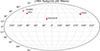 |
Fig. 1. J-PAS IDR202406 observed footprint with all the filters showing the positions of the seed fields. The coordinates (RA, Dec.) in degrees are: CODEX (126.1125, 40.1053), miniJPAS (214.4500, 52.7261), JPSV (244.00, 43.00), and StephQuint (339.00, 22.50). |
The observations were reduced using a dedicated pipeline developed at Centro de Estudios de Física del Cosmos de Aragón (CEFCA) for processing images from the two main telescopes of the OAJ: JST250 and JAST80. This data reduction pipeline has already been successfully used in the processing of previously released datasets, such as J-PLUS (Cenarro et al. 2019; López-Sanjuan et al. 2024) and miniJPAS (Bonoli et al. 2021). Photometric calibration (Vázquez-Ramiró et al. in prep.) was done using Gaia Data Release 3 (Gaia Collaboration 2023).
3. Methodology
Identifying EELGs presents a challenge due to their low number density and the growing volume of data, which make traditional methods inefficient. With J-PAS, we can now adopt a more powerful approach, taking advantage of both the spectrophotometric information and the 54 narrow-band images available for each source. In this work we propose combining a traditional search method with a machine learning approach to efficiently handle large datasets and improve the identification of EELGs in current and future data releases.
3.1. Step I: Classical search
The J-PAS catalogue contains a vast number of objects that need to be filtered. To begin the process, we designed an operational flow that ensures specific criteria are met to determine whether or not a source should be included. The photo-spectrum is first processed by removing emission lines or artefacts using 3-sigma clipping, followed by a polynomial fit (of first and second degrees, with the best fit chosen based on root mean square error) to model the continuum. This step is repeated three times, taking into account the uncertainties in each data point: once for the upper limit, once for the lower limit, and once for the standard data points. In this way, we ensured a robust measurement of the continuum level for galaxies where it is reliably detected.
To avoid false detections driven by noise, we required that an emission line have a flux at least 5σcont above the continuum, where σcont represents the standard deviation of the continuum level in the vicinity of the line. This criterion ensures that lines are not buried in the spectral noise and helps avoid spurious detections in noisy spectra. While this threshold increases the reliability of the line detection and the measurement EWs, it may limit our ability to identify EELGs in cases where the continuum is too faint or not detected with sufficient confidence. However, this trade-off is necessary to ensure that derived EWs are not artificially boosted by an underestimated or noisy continuum. Next, following Iglesias-Páramo et al. (2022), we applied the contrast factor to select only those sources EW greater than 300 Å. The criterion is defined as
 (1)
(1)
where EW is 300 Å and ΔF is the filter width. The choice for 300 Å facilitates the identification of young, low-metallicity galaxies undergoing intense starburst episodes. Other minor conditions are: a signal-to-noise ratio (S/N) lower than 8 in individual measurements, and fluxes in the band lower than 3 × 10⁻¹⁵ erg s−1 cm−2 Å−1 or negative are discarded. We did not apply a criteria to separate stars from galaxies because EELGs are often extremely compact, and classifiers can sometimes become confused with stars (e.g. Cardamone et al. 2009), leading to misclassification.
3.2. Step II: Active galactic nucleus/quasar and cosmetic defects
After applying Step I, we expected to obtain a clean sample of galaxies with well-defined emission lines and EW greater than 300 Å. However, some contaminants may still remain in the sample. For instance, there are cases where the polynomial continuum fit (of first or second degree) fails, leading to an incorrect continuum estimation, such as in star-like spectra. Additionally, certain objects can show spurious emission features due to contamination in a specific band, for example diffraction spikes, which can artificially boost the flux and mimic an emission line. Moreover, quasi-stellar objects (QSOs) can also appear in the sample due to their strong emission lines; however, our goal is to identify emission lines produced by star formation, not those associated with QSO activity. To minimize these sources of contamination, we trained a neural network (NN) to distinguish EELGs from other types of objects.
We normalized the photo-spectra to a range of [0, 1] by dividing each spectrum by its maximum flux value. This normalization is done independently for each object, and thus the photo-spectra are normalized with respect to their own maximum. This procedure ensures consistent input scaling for the NN, but it does not preserve absolute flux information. As such, the normalization is relative (not physically calibrated) and is primarily intended to facilitate efficient NN training. The training sample consists of 684 sources labelled as EELGs, carefully selected to build a representative and reliable EELG dataset. These galaxies were initially identified using the photometric selection method described in Iglesias-Páramo et al. (2022). Each candidate was then visually inspected to confirm its nature and ensure it met the established EELG selection criteria mentioned above. It is precisely during this manual inspection step that the need for automated methods becomes evident: while feasible for a few hundred sources, visual confirmation quickly becomes impractical when scaling up to the full J-PAS dataset. In addition to labelled EELGs, the training set includes 1160 sources labelled as non-EELGs. This group comprises a diverse set of objects, including spectroscopically confirmed QSOs, obtained by cross-matching J-PAS with the DESI DR1 catalogue (DESI Collaboration 2025), as well as a variety of normal galaxies, such as elliptical, late-type, and spiral galaxies. These non-EELG sources serve as a contrasting population that enables the model to learn to distinguish EELGs from other types of galaxies and active objects. As the classes in the training set are not balanced, we applied class weights inversely proportional to the number of instances in each class to mitigate bias during training. Additionally, 70% of the dataset is used for training, while the remaining 30% is reserved for testing and performance evaluation, remaining unseen by the network during training.
To quantify the likelihood of a galaxy being an EELG, our primary NN outputs an ‘EELGness’ score, denoted as P0, ranging from 0 to 1, where higher values indicate a stronger probability of being a true EELG. This network processes both the photometric spectrum and the galaxy image, following the architecture shown in Fig. B.1, but considering only the upper and middle branches (spectral and image processing). However, during visual inspection of the galaxy images, we identified a significant number of false positives caused by cosmetic defects artefacts in the imaging data that produce emission-line-like features but do not correspond to real astrophysical objects. To address this, we developed a second NN, specifically trained to distinguish between true EELGs and these cosmetic artefacts. This network outputs a complementary score, P1, which reflects the probability that a given detection is a genuine EELG and not a cosmetic defect. The two networks have the same fundamental architecture, with one key difference: the cosmetic-defect classifier includes an additional dedicated branch (Fig. B.1, lower branch) designed to analyse image regions associated with the location of the emission line, improving the network’s ability to recognize defects. For the standard EELG classifier (P0), only the first two branches (spectral and image) are active. For the cosmetic-defect classifier (P1), all three branches are used, including the defect-detection branch. In both cases, the outputs of the active branches are concatenated and passed through a common set of dense layers, which integrate the extracted features and produce the final classification output. This design ensures that both spectral and morphological information, as well as potential image artefacts, are jointly considered for more reliable EELG identification. A deep description of the architecture and training of the NN is shown in Appendix B.
4. Sample selection and characterization
We selected galaxies with P0 ≥ 0.8, ensuring a well-balanced trade-off between completeness and purity. This threshold allows us to recover nearly 97% of extreme emission line emitters in the test sample, as determined from the classifier’s performance on a labelled test set. Applying P1 > 0.2 reduces the sample from 969 to 917 galaxies, eliminating possible fake detections in the images. Of the final sample, 79 galaxies have counterparts in the latest release of the DESI DR1 catalogue (Fig. 2). Assuming that the DESI selection is not strongly biased for or against EELGs, we can assess the completeness of our selection by examining how many DESI sources with EW greater than 300 Å in at least one of the emission lines, fall within the J-PAS footprint and among those, how many are successfully recovered by our method. A total of 28 DESI EELGs sources lie within the J-PAS footprint. Eight out of 28 are not present in the J-PAS catalogues: seven correspond to starburst regions in large spiral galaxies, and one object with an I-band magnitude fainter than 23.5, which exceeds the J-PAS limiting value. Among the 20 DESI EELGs within the J-PAS catalogue, 16 are successfully recovered by our selection methodology. The remaining four galaxies are not detected because they do not satisfy the EW criteria in J-PAS. This is the case of some cometary or tadpole blue compact dwarfs (e.g. Papaderos et al. 2008; Sánchez Almeida et al. 2015), in which the emission line EW of the compact starburst spectrum captured by the DESI fibre is different from the EW measured by the J-PAS aperture photometry, which in those cases includes part of the faint cometary or tadpole tail with a less extreme spectrum, i.e. fainter nebular contribution. Additionally, DESI targets compact sources by placing the spectroscopic aperture on the brightest knot within the galaxy, which often results in high EW measurements. In contrast, when the photometric measurement is integrated over the entire galaxy, the EW can be significantly diluted due to the contribution of the older, underlying stellar population. This distinction arises from the very definition of an EELG: in our approach, we did not define an EELG as a galaxy that merely hosts a burst, but rather as a galaxy in which the burst dominates the optical luminosity, outshining the additional contribution of older stellar populations from the host galaxy (e.g. Amorín et al. 2009, 2012; Fernández et al. 2022). Following our selection criteria, we recovered all the EELGs within the J-PAS footprint, with the exception of the faint object.
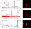 |
Fig. 2. Data products from J-PAS for the EELG candidates. Left: J-PAS photometric spectrum (black line) and the corresponding DESI spectrum (red line). The shaded grey region marks the wavelength range selected for integration. Right: Image cutouts resulting from integrating the data cube over the selected spectral region. The horizontal white bar is 2 arcseconds in length. With J-PAS we are able to detect the continuum, but not with DESI. |
4.1. Purity and AGN contribution
To assess active galactic nucleus (AGN) contribution, we employed the Baldwin–Phillips–Telervich (BPT) diagram with the sources that have a counterpart in DESI DR1 (Fig. 3). Emission lines of the DESI spectra were measured with the LIME tool (Fernández et al. 2024), revealing three AGN candidates showing broad components in Balmer lines. Additionally, we identified two galaxies exhibiting [Ne V] λ3426 emission, a reliable AGN tracer. Although rare, [Ne V] has also been detected in low-metallicity star-forming galaxies (Izotov et al. 2021; Mingozzi et al. 2025; Arroyo-Polonio et al. 2025). This brings the total AGN contamination to 5 out of 79 galaxies, or approximately 6%. Theses sources were removed from the sample. As shown later (Sect. 4.3, Fig. 6), the spectroscopic and J-PAS samples exhibit similar properties, suggesting that the overall AGN contamination in our selection is around 6%.
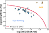 |
Fig. 3. BPT diagram (Baldwin et al. 1981). Blue points are data points that have a counterpart in DESI with the Hα. The data points classified as AGNs are plotted in orange. The solid red line corresponds to the Kewley relationship (Kewley et al. 2001). |
4.2. Redshift estimation
In J-PAS photometric redshifts are computed for all sources with i < 22.5 using galaxy templates regardless of their morphological classification. This approach means that the resulting redshift probability distributions, P(z), are conditional on the object being a galaxy. Such a method enables galaxy number density calculations that incorporate uncertainties in the morphological classification (Hernán-Caballero et al. 2021) and, in our case, the construction of a complete EELG sample unbiased by morphology.
We used a customized version of LePhare (Arnouts & Ilbert 2011), keeping the same configuration as used in the official photo-z runs for the miniJPAS PDR (Hernán-Caballero et al. 2021) and J-NEP (Hernán-Caballero et al. 2023), except for the addition of two specific EELG templates, which are described below. LePhare employs filter transmission profiles to compute synthetic photometry as a function of redshift for a given set of templates. EELGs, being rare and peculiar objects, require dedicated templates with detailed nebular emission features to accurately determine their redshift. We constructed spectroscopic templates based on a selection of AGNs and star-forming galaxies from the DESI early data release.
These templates span a wavelength range from 1400 Å to 10000 Å, covering the wavelength range of J-PAS filters set until redshift ≈0.9. They include representative spectral energy distribution (SED) of EELGs, particularly those exhibiting strong [O III] and Hα emission. This inclusion is crucial for accurate photometric redshift estimation, as standard template libraries used in photo-z codes like LePhare often lack examples of galaxies with such intense emission lines. To build these templates, we performed a stacking analysis of over 12 997 star-forming galaxies and 350 AGNs selected from the DESI spectroscopic sample. This approach allowed us to construct realistic SEDs that capture both the continuum and emission line features characteristic of EELGs. Excluding these templates slightly degrades the overall agreement between photometric and spectroscopic redshifts, particularly in cases where the algorithm confuses [O III] with Hα. Further details on the DESI sample selection and template construction will be provided in Bonatto et al. (in prep.). Using these optimized templates, we find excellent agreement between the best-fit photometric redshifts from LePhare and the spectroscopic redshifts across the full redshift range up to z ≈ 0.9, as illustrated in Fig. 4. To quantify the photometric redshift accuracy, we computed the normalized median absolute deviation (σNMAD), obtaining a value of 0.0015, which is five times lower than that obtained without using the templates.
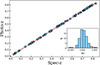 |
Fig. 4. 1:1 correlation observed between the spectroscopic redshifts and the best-fit values from LePhare. The inset quantifies the relative differences between the two redshift estimates. |
Moreover, the redshift distribution of our sample is remarkably homogeneous (Appendix A.1), ensuring that our analysis is not biased by redshift-dependent effects. As an additional diagnostic, we examined the template type preferred by the redshift fitting. We find that 5% of the galaxies are better fitted by an AGN template, which is fully consistent with our previous estimate of AGN contamination in the sample.
4.3. SED fitting
To compute the physical properties, we made use of Code Investigating GALaxy Emission (CIGALE v2025.0; Boquien et al. 2019). CIGALE uses parametric star formation histories and outputs physical parameters and their uncertainties by using a Bayesian approach. It creates a probability distribution function for each parameter by evaluating the χ2 over the full set of models used for the fit. In this work the star formation history was modelled, as in previous works (e.g. Lumbreras-Calle et al. 2022), using a double exponential with an old population selected to represent the underlying galaxy, and a young one to reproduce the strong starburst, inducing the extreme emission lines. In addition to the J-PAS photometric points, we incorporated complementary photometric data that cover the UV and IR regimes. Specifically, we included the far-UV and near-UV bands from the Galaxy Evolution Explorer (GALEX) telescope; the u, g, r, i, z bands from the SDSS; the Wide-Field Infrared Survey Explorer (WISE) bands at 3.4, 4.6, 12.1, and 22.2 μm; the Spitzer Infrared Array Camera (IRAC) bands at 3.6, 4.5, 5.8, and 8 μm; and Spitzer Multiband Imaging Photometer for Spitzer (MIPS) bands at 24 and 70 μm. For the stellar population synthesis, we used the Charlot & Bruzual (2019) models with the Chabrier (2003) initial mass function. Nebular emission is incorporated using the CLOUDY models (Ferland et al. 2013), and we assumed a fesc = 0.0, meaning that all LyC photons are reprocessed into the Balmer lines, fdust = 0 (no LyC absorbed by dust) and an electron density ne = 100 cm−3. The attenuation in the models was taken into account by using the modified Calzetti et al. (2000) law and for the dust emission we used the models by Dale et al. (2014). These extended photometric data improve the constraints on the SEDs, particularly in the UV, where they help characterize recent star formation, and in the IR, where they are essential to account for dust emission and reprocessed light. All the parameters employed in the fitting process are summarized in Table C.1.
We estimated the continuum, stellar mass, star formation history, and extinction in order to properly characterize the sample. In Fig. 5 the main sequence (MS) of star forming galaxies is shown. Notably, our selected sample of EELGs is composed of galaxies with high SFRs, above the star-forming MS at redshift z ∼ 4.5–5, derived using BAGPIPES (Carnall et al. 2018) in Cole et al. (2025). This result assumes a Chabrier (2003) initial mass function and applies the Calzetti et al. (2000) dust attenuation law. This was expected, as we selected galaxies with high EW, a characteristic feature of bursty galaxies, where their last burst of star formation occurs within the last 10 Myr.
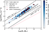 |
Fig. 5. MS of star-forming galaxies. The plot shows the logarithm of the SFR, log(SFR10), versus the logarithm of the stellar mass, log(M★). The SFR10 refers to the average SFR over the past 10 Myr. Red points indicate galaxies with spectroscopic observations from DESI. The dotted black line shows the relation from Cole et al. (2025) at redshift 4.5–5. The solid black line corresponds to the relation from Curtis-Lake et al. 2021 (mock photometric samples of galaxies at z ≈ 5), the dot-dashed line the relation from Speagle et al. (2014), 64 measurements of the star-forming ‘MS’ from literature out to z ≈ 6), and the pink line the results from the Millennium Simulation (Springel et al. 2005). The dashed lines draw regions of constant sSFRs at values of −7 and −9. |
Most galaxies fall within the 7 < log(M★/M⊙) < 10 with a median of log(M★/M⊙) = 8.66 ± 0.02. In comparison, the spectroscopic subsample yields a median mass of log(M★/M⊙) = 8.98 ± 0.09. The spectroscopic counterpart appears slightly burstier (SFR10), with a mean SFR of 0.97 ± 0.02 M⊙ yr−1 in the full sample and 1.27 ± 0.13 M⊙ yr−1 in the DESI subsample. Moreover, most galaxies show relatively low dust extinction, with a median colour excess parameter of E(B − V)J − PAS = 0.25 ± 0.01 and E(B − V)DESI = 0.22 ± 0.01. To assess whether the two populations can be statistically considered equal, we performed a Kolmogorov-Smirnov test with 1000 Monte Carlo draws to account for uncertainties. The results indicate that although the SFR and stellar mass distributions show small but statistically significant differences (p < 0.05), the sSFR over the recent 10 Myr (sSFR10) and E(B − V), shows no significant deviation between J-PAS and spectroscopy sample (p > 0.05). This indicates that the relative scaling between the SFR and mass is preserved and that the samples are consistent with representing the same underlying galaxy population in terms of star-formation activity (see Fig. 6). The mild differences that we can appreciate might be attributed to the fibre selection function in DESI.
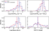 |
Fig. 6. Histogram of the SFR10, sSFR10, stellar mass (M⊙), and extinction (E(B − V) for the J-PAS sample and its DESI counterparts. Vertical dashed lines indicate the mean values of each distribution. |
Derived SED parameters for selected galaxies.
4.4. Emission line flux extraction
One of the main spectral features of EELGs is their strong emission lines; thus, capturing precise and robust measurements of line intensities is essential. Measuring fluxes using photometric bands is particularly challenging due to the limited spectral resolution (R ≈ 60) and it requires precise modelling of both the stellar continuum and the line contribution to accurately recover the total flux. Additionally, factors such as the non-uniform transmission curve of filters, potential overlap of multiple emission lines within a single filter, the intrinsic width of the emission lines and inaccuracies in the photometric redshift, can introduce significant uncertainties. To address these challenges, we adopted the following strategy for estimating the fluxes of Hα, Hβ, and [O III].
First, we modelled each emission line assuming a Gaussian profile with a conservative width of σ = 7 Å to account for thermal broadening and instrumental effects. For reference, studies of giant HII regions in the context of the L–σ relation report typical σ values of ∼3 Å (e.g. Terlevich & Melnick 1981). This is significantly narrower than the width assumed in our modelling, which ensures that our flux estimation is robust against potential flux losses of the wings of the emission line. After that, to guarantee that a given spectral line is fully captured by a specific filter, we checked that at least 95% of the modelled line flux lies within the transmission curve of each filter. If this condition is met, we assumed the total line flux is correctly captured.
To isolate the emission line flux from the underlying stellar continuum, we first estimated the continuum level using the best-fit SED model provided by CIGALE. This model was then convolved with the transmission curves of the J-PAS filters to obtain a realistic prediction of the continuum flux in each band. Finally, the continuum contribution was subtracted from the observed flux in the filter where the emission line was detected. Each line has certain singularities that must be considered:
-
Hα: The easiest line to estimate because it is largely isolated except for the nearby [N II] doublet. We corrected for this contamination by assuming a typical flux ratio of [N II]λλ6548, 6583/Hα ≈ 0.07, which provides a reasonable approximation for EELGs. This ratio was derived from an empirical analysis of all the sample of star-forming galaxies extracted from the DESI spectroscopic dataset, as presented in Bonatto et al. (in prep.). Consistent values are obtained when using the sample of EELGs from Pérez-Montero et al. (2021). This correction should be applied only when the S/N is high enough to detect [NII]. However, we applied it to all galaxies despite the possibility that the flux is underestimated in some cases.
-
[O III] λ5007: Ideally, we selected a filter where the line is well isolated from [O III] λ4959 to avoid blending. If this is not possible, we measured the combined flux of the two lines and applied the theoretical ratio [O III] λ4959 = 1/2.95 × [O III] λ5007 to disentangle its contribution.
-
Hβ: It is generally straightforward, but special care must be taken in cases where the nearby [O III]λ4959 line may contaminate the observed flux. When Hβ and [O III]λ4959 fall within the same filter, we determined whether [O III]λ5007 was detected in isolation in an adjacent filter. If so, we estimated its flux and assume the theoretical line ratio to correct for the contribution of [O III]λ4959 to the blended Hβ+[O III]λ4959 measurement. This allowed us to recover a physically consistent estimate of the Hβ flux while ensuring that the [O III] lines are treated in a coherent manner.
In Fig. 7 we compare the fluxes obtained with J-PAS to those measured in the DESI DR1 catalogue using LIME as a fitting line tool with S/N > 3. The DESI fluxes have not been aperture-corrected, as most sources are compact and the nebular emission fits within the 1.5″ diameter fibre. Overall, the emission line fluxes derived from photometric bands are consistent with spectroscopic measurements within the errors (σNMAD < 0.09 dex).
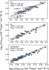 |
Fig. 7. Photometric fluxes compared with the spectroscopic fluxes from the DESI counterpart for Hβ, Hα, and [O III] 5007 Å (from top to bottom). Grey lines indicate de limits of the ±1σ region. The red line represents the 1:1 ratio. |
Computed emission line quantities for selected galaxies.
4.5. Line flux equivalent widths
To compute the EW, we first convolved the synthetic stellar and nebular continuum models derived from CIGALE with the transmission curve of the J-PAS filters. This allowed us to estimate the continuum flux within each filter. We then calculated the EW using the measured flux in the filter using the expression
![Mathematical equation: $$ \begin{aligned} \text{ EW} \,[\AA ] = \frac{\text{ Flux} - \text{ Cont.}}{\text{ Cont.}} \times \Delta , \end{aligned} $$](/articles/aa/full_html/2026/02/aa57358-25/aa57358-25-eq10.gif) (2)
(2)
where Δ represents the filter effective width. This assumes a flat continuum across the filter and may introduce differences with respect to spectroscopic measurements. The mean EWo for the full sample is 665 Å in [O III] λ5007 and 383 Å in Hα. However, there are instances where the EW is above 300 Å in [O III] λ5007 but not in Hα, and viceversa. In Fig. 8, the histograms for EW of [O III] λ5007 and Hα are shown. The peak observed around 300 Å is a consequence of our selection criteria, which impose a minimum EW threshold as part of the methodology. This effectively cuts the original distribution. Since objects with high EWs are rare, this selection removes the low EW part of the distribution, where most objects lie, resulting in an artificial peak at 300 Å. Also, the threshold value in EW was imposed on non rest-frame spectra with unknown redshift at that time, so it is normal that some objects appear below that limit. In Fig. 9 we compare the pure photometric measurement of EW (S/N > 3) with the values drawn for their spectroscopic counterparts. We observe a very good agreement between the two, with consistent results. The larger error bars in the spectroscopic sample are attributed to the lower continuum levels in these galaxies compared to their J-PAS counterparts. This difference in continuum strength affects the precision in the spectroscopic measurements, leading to increasing uncertainties.
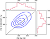 |
Fig. 8. Contour plot of the EWs of Hα and Hβ. Red histograms show the individual distributions along each axis. The contours represent the density of sources in the EW(Hα)–EW(Hβ) plane. Percentage shows the accumulative distribution and the grey line the 1:1 correlation. |
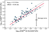 |
Fig. 9. J-PAS EW compared with the spectroscopic EW from the DESI counterpart for [O III] λ5007 Å line emission. White triangles are upper limits. Grey lines indicate the limits of the ±1σ region. |
5. Discussion
In this section we investigate the ionizing photon budget of our EELG sample. The production of ionizing photons is dominated by very young and hot massive stars, whose presence is linked to the strength of nebular emission lines. In particular, high [O III]λ5007 EWs trace bursts of star formation and therefore correlate with the stellar population and the ionizing photon production efficiency (ξion). Age is also expected to correlate with ξion, since younger stellar populations host larger numbers of hot, massive stars capable of producing ionizing radiation. Exploring these relationships in local EELGs provides a way of interpreting the conditions under which galaxies can contribute to the ionizing budget.
5.1. The ionizing rate of EELGs
ξion, quantifies the number of hydrogen-ionizing photons emitted per unit of UV continuum luminosity at 1500 Å. It measures how efficiently young hot stars convert their UV light into ionizing radiation capable of affecting the surrounding gas. Together with the cosmic SFR density (ρSFR) and the escape fraction of LyC photons (fesc), it is possible to estimate the rate of ionizing photons that are produced and successfully escape into the intergalactic medium (Robertson et al. 2015). Primeval galaxies with strong bursts of star formation emit significant amounts of photoionizing radiation, suggesting that they are key agents for the re-ionization of the Universe (Trebitsch et al. 2017; Finkelstein et al. 2019). Thus, studying ξion helps us assess the capability of EELGs, to drive cosmic re-ionization. In this context, EELGs in the local Universe provide valuable analogues to high-redshift systems. These galaxies often exhibit compact morphologies, low metallicities, hard radiation fields and high sSFRs. Moreover, several EELGs have shown direct detections of LyC leakage with significant escape fractions (fesc ≳ 0.1; Izotov et al. 2016, 2018; Flury et al. 2022b,a; Vanzella et al. 2016). We evaluated the ionizing photon production efficiency as
 (3)
(3)
where N(H0) is the ionizing photon rate in s−1 and LUV is the UV luminosity density at 1500 Å, which we estimated from CIGALE models assuming a filter band of 100 Å centred at 1500 Å. Just to clarify, LUV is computed over the entire model, so there will be a (small) contribution from nebular continuum emission included along with the stellar population. To estimate the ionizing photon rate, we used the dust-corrected Hα luminosity from Leitherer & Heckman (1995), assuming that no ionizing photons escape the galaxy and that case B recombination applies. Additionally, we utilized the dust-corrected Hβ luminosity, as it enabled us to cover a wider range of redshifts:
 (4)
(4)
This equation exhibits a mild dependence on temperature and metallicity (Charlot & Longhetti 2001), and is also sensitive to the assumed initial mass function and stellar metallicity (Atek et al. 2022; Wilkins et al. 2019). The derived value of ξion should be considered a lower limit as we assumed fesc = 0 for a radiation-bounded nebula, for example. When the escape fraction increases, not all ionizing photons are reprocessed into Balmer emission lines, which leads to an increase in ξion by a factor of 1/(1 − fesc). We only considered ξion values to be reliable when Balmer lines are detected with a S/N > 3.
5.2. Ionizing rate versus EW (O III])
The EW of [O III] λ5007 has often been used as a proxy for ξion. Chevallard et al. (2018) established this relation using local analogues from SDSS, selected to resemble high-redshift galaxies. More recent studies have confirmed a positive correlation between EW([O III])λ5007 and ξion in high-redshift samples: Simmonds et al. (2024) analysed 677 galaxies at z ∼ 4–9 using JWST/NIRCam photometry, Llerena et al. (2024a) examined a sample of 761 galaxies at 4 ≤ z ≤ 10 from various JWST surveys, and Pahl et al. (2025) studied 163 galaxies spanning 1.06 < z < 6.7. Additionally, Tang et al. (2019) focused on a sample of extreme [O III] emitters at z = 1.3–2.4. In Fig. 10 we show that this trend is consistent with our data. We performed a linear fit to the observed correlation between log(EW0 [O III]) and log(ξion) using a Markov chain Monte Carlo approach. The resulting best-fit relation is
![Mathematical equation: $$ \begin{aligned} \log (\xi _{\mathrm{ion}})\,(\mathrm{Hz\,erg}^{-1})&= (0.69 \pm 0.15) \times \log (\mathrm{EW}_0\, \mathrm{[O\,III]})\nonumber \\&+ (23.35 \pm 0.06). \end{aligned} $$](/articles/aa/full_html/2026/02/aa57358-25/aa57358-25-eq13.gif) (5)
(5)
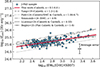 |
Fig. 10. Relation between the ionizing photon production efficiency, log(ξion), and the rest-frame EW of [O III], log(EW0 [O III]). The blue points represent our sample of EELGs, with a typical error bar shown in the lower right region. The solid red line indicates the best-fit linear relation obtained in this work using a Markov chain Monte Carlo approach, with the shaded area showing the 1σ confidence interval. For comparison, previous relations from the literature are also shown: Tang et al. (2019), dashed), Pahl et al. (2025), dotted), Simmonds et al. (2024), dash-dotted), Llerena et al. (2024b), solid), and Begley et al. (2025), solid with dot.) |
This relation confirms a moderate positive correlation, where galaxies with stronger EW ([OIII]) tend to have higher ionizing photon production efficiencies. The slope of ∼0.69 is consistent with recent findings in the literature, though slightly shallower than some previous works (Begley et al. 2025; Pahl et al. 2025; Simmonds et al. 2024; Llerena et al. 2024b; Tang et al. 2019). This supports the idea that EW([O III]) can serve as a useful proxy for identifying galaxies with elevated ionizing output.
An important consideration in this work is the choice of extinction law. We adopted the attenuation curve from Calzetti et al. (2000), with RV = 4.05, to ensure consistency with previous studies and with the SED fitting approach implemented in CIGALE. However, several studies have suggested that a steeper attenuation law lacking the UV bump and characterized by lower values of RV, typically around RV ∼ 2.7, may be more appropriate for compact, star-forming galaxies at high redshifts (Shivaei et al. 2020; Reddy et al. 2018; Izotov et al. 2017). Adopting a Small Magellanic Cloud-type extinction law can lead to increases of up to 0.3 dex in the derived values of ξion. However, when running CIGALE with a steeper attenuation curve (e.g. Small Magellanic Cloud-like, with RV ∼ 2.7), we found that the uncertainties in the estimated E(B − V) values increased significantly, resulting in larger uncertainties in the inferred ξion. Additionally, CIGALE assumes a single attenuation law for both stellar and nebular emission, applying the same E(B − V) correction to both components in the dustatt_calzleit module. This differs from the typical spectroscopic approach, where the stellar UV continuum is corrected using Calzetti or Small Magellanic Cloud-type laws based on SED fitting, while the nebular lines are corrected using the Cardelli et al. (1989) law together with the Balmer decrement. However, due to our instrumental constraints in particular, the inability to measure Hα for galaxies at z ≳ 0.4 and the added uncertainties that would result from propagating errors in both Hα and Hβ, we adopted the extinction derived from SED fitting to correct both the continuum and line emission. While this introduces some systematic uncertainty, it provides a consistent and homogeneous framework for estimating ξion across our full sample.
5.3. Ionizing rate versus age
We find that ξion shows a strong correlation with both EW([O III]) and EW(Hβ) (see Fig. 11), a trend consistent with previous studies in the literature. The correlation with EW(Hβ) is particularly pronounced. According to models (e.g. Starburst99; Leitherer et al. 1999; Hawcroft et al. 2025), the EW of Hβ is a reliable tracer of the age of a starburst, reaching maximum values (greater than 200 Å) within the first 3–4 Myr and declining rapidly afterwards. In Fig. 11 we illustrate the relationship between EW(Hβ) and the ionizing photon production efficiency. Our results strongly suggest that galaxies dominated by younger bursts exhibit the highest efficiencies. This aligns with expectations for high-redshift galaxies, where star formation tend to be stochastic and/or bursty (e.g. Sun et al. 2023; Pallottini & Ferrara 2023; Dressler et al. 2024):
![Mathematical equation: $$ \begin{aligned} \log \!\left(\xi _{\mathrm{ion}}\right)\,[\mathrm{Hz\,erg}^{-1}]&= (0.643 \pm 0.063)\times \log \!\left(\mathrm{EW}_0(\mathrm{H}\beta )\right) \nonumber \\&\quad + (23.87 \pm 0.12). \end{aligned} $$](/articles/aa/full_html/2026/02/aa57358-25/aa57358-25-eq14.gif) (6)
(6)
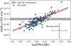 |
Fig. 11. Relation between the ionizing photon production efficiency, log(ξion), and the rest-frame EW of Hβ, log[EW0(Hβ)]. The blue points represent our sample. The shaded grey region marks the commonly adopted threshold (log(ξion) > 25.3). |
The commonly adopted threshold of log10(ξion/erg−1 Hz)∼25.3 (Robertson et al. 2015) identifies galaxies capable of significantly contributing to the ionizing photon budget required for cosmic re-ionization. A fraction of the J-PAS EELGs exceed this limit. Notably, galaxies hosting the youngest bursts, are precisely those that reach or surpass this threshold, reflecting their intense production of LyC photons. This directly links these young bursts to the cosmic re-ionization budget, as they can provide a significant fraction of the photons necessary to ionize the intergalactic medium. Current evidence suggests that the ξion of these low-redshift EELGs is comparable to that of galaxies at z > 6, implying little evolution of this parameter across cosmic time.
6. Conclusions
In this work we present a novel method for the photometric identification of EELGs based on EW, combining a classical approach (measuring the EW directly from narrow-band photometry) with the application of artificial intelligence techniques. The selection method relies on detecting strong emission lines, specifically those with rest frame EWs([O III]) or EWs(Hα) greater than 300 Å, by measuring the contrast between J-PAS narrow-band filters and the estimated continuum. Using data from the J-PAS IDR202406, we applied this methodology to select a sample of 917 EELGs up to a redshift of z = 0.8, over an area of ≈30 deg2. Our selection achieves a purity of 95%, with an estimated AGN contamination of only 5%, and a completeness of 96%, as determined via comparisons with DESI spectroscopic counterparts. With these criteria, we find a density of 31 EELGs per square degree-nearly doubling the density reported in the miniJPAS study by Iglesias-Páramo et al. (2022), who identified 17 EELGs per square degree.
We carried out SED fitting using the CIGALE software to characterize the physical properties of the galaxies. Most of the sources have stellar masses in the range 107–1010 M⊙, with a median value of log(M★/M⊙) = (8.66 ± 0.02). Furthermore, we are able to recover a population of low-mass galaxies with stellar masses below 107 M⊙, which are not accessible to DESI. This bias is probably due to the DESI sample selection. One of the main advantages of J-PAS is the absence of selection biases, except for those inherently linked to the survey’s magnitude limit (the Malmquist bias). We used specific templates to accurately retrieve the photometric redshifts, achieving excellent agreement with the spectroscopic redshifts; this gives us confidence in the physical parameters we derived, such as line fluxes and ξ. Ionizing photon production is particularly important during the epoch of re-ionization. Nearby galaxies that exhibit physical characteristics reminiscent of early-Universe systems, often referred to as local analogues, offer a unique window into the conditions that regulate ionizing photon output. Their compact structure, intense star formation, and low chemical enrichment make them the perfect systems to study to determine what physical conditions lead to efficient ionizing photon production and how those photons might escape into the surrounding medium. Our selected J-PAS EELG sample provides a solid starting point for an unbiased study of local analogues, with most sources exceeding the minimum efficiency required to re-ionize the Universe ( ) at z > 6.
Our method offers an efficient way to identify EELGs using narrow-band photometry. The selected sample helps us understand the physical conditions that led to efficient ionizing photon production in galaxies similar to those from the early Universe. A spectroscopic follow-up of these sources will shed light on photon escape mechanisms and their nebular physical properties and chemical abundances. The presented catalogue will be extended as new J-PAS data become available.
Data availability
Full Tables 1 and 2 are available at the CDS via https://cdsarc.cds.unistra.fr/viz-bin/cat/J/A+A/706/A261
Acknowledgments
We thank the referee for several helpful suggestions. AGA, MGO and IM acknowledge financial support from the Severo Ochoa grant CEX2021-001131-S, funded by MICIU/AEI/10.13039/501100011033. AGA also acknowledges FPI support under grant code CEX2021-001131-S-20-7. Both AGA and MGO acknowledge support from the research grant PID2022-136598NB-C32 (“Estallidos8”). MGO also acknowledges the support by the project ref. AST22_00001_Subp_11 funded from the EU – NextGenerationEU. RA acknowledges support from PID2023-147386NB-I00 funded by MICIU/AEI/10.13039/501100011033 and ERDF/EU. IM acknowledges support from PID2022-140871NB-C21 funded by MICIU/AEI/10.13039/501100011033 and FEDER/UE. RGD acknowledge financial support from the project PID2022-141755NB-I00, and the Severo Ochoa grant CEX2021-001131-S funded by MICIU/AEI/ 10.13039/501100011033. JAFO and AE acknowledge support from the Spanish Ministry of Science and Innovation and the EU–NextGenerationEU through the RRF project ICTS-MRR-2021-03-CEFCA. AHC and ALC acknowledge support from MCIN/AEI/10.13039/501100011033, “ERDF A way of making Europe”, and “EU NextGenerationEU/PRTR” through PID2021-124918NB-C44 and CNS2023-145339, as well as from the RRF project ICTS-MRR-2021-03-CEFCA ALC and RPT acknowledge the financial support from the European Union – NextGenerationEU through the RRF program Planes Complementarios con las CCAA de Astrofísica y Física de Altas Energías – LA4. I.B. acknowledges support from the EU Horizon 2020 programme (Marie Sklodowska-Curie Grant 101059532) and the Franziska Seidl Funding Program, University of Vienna. This paper has gone through internal‘ review by the J-PAS collaboration. Based on observations made with the JST/T250 telescope and JPCam at the Observatorio Astrofísico de Javalambre (OAJ), in Teruel, owned, managed, and operated by the Centro de Estudios de Física del Cosmos de Aragón (CEFCA). We acknowledge the OAJ Data Processing and Archiving Unit (UPAD) for reducing and calibrating the OAJ data used in this work. Funding for the J-PAS Project has been provided by the Governments of Spain and Aragón through the Fondo de Inversiones de Teruel; the Aragonese Government through the Research Groups E96, E103, E16_17R, E16_20R, and E16_23R; the Spanish Ministry of Science and Innovation (MCIN/AEI/10.13039/501100011033 y FEDER, Una manera de hacer Europa) with grants PID2021-124918NB-C41, PID2021-124918NB-C42, PID2021-124918NA-C43, and PID2021-124918NB-C44; the Spanish Ministry of Science, Innovation and Universities (MCIU/AEI/FEDER, UE) with grants PGC2018-097585-B-C21 and PGC2018-097585-B-C22; the Spanish Ministry of Economy and Competitiveness (MINECO) under AYA2015-66211-C2-1-P, AYA2015-66211-C2-2, and AYA2012-30789; and European FEDER funding (FCDD10-4E-867, FCDD13-4E-2685).
References
- Amorín, R., Aguerri, J. A. L., Muñoz-Tuñón, C., & Cairós, L. M. 2009, A&A, 501, 75 [NASA ADS] [CrossRef] [EDP Sciences] [Google Scholar]
- Amorín, R. O., Pérez-Montero, E., & Vílchez, J. M. 2010, ApJ, 715, L128 [CrossRef] [Google Scholar]
- Amorín, R., Pérez-Montero, E., Vílchez, J. M., & Papaderos, P. 2012, ApJ, 749, 185 [CrossRef] [Google Scholar]
- Amorín, R., Sommariva, V., Castellano, M., et al. 2014, A&A, 568, L8 [CrossRef] [EDP Sciences] [Google Scholar]
- Amorín, R., Pérez-Montero, E., Contini, T., et al. 2015, A&A, 578, A105 [NASA ADS] [CrossRef] [EDP Sciences] [Google Scholar]
- Arnouts, S., & Ilbert, O. 2011, Astrophysics Source Code Library [record ascl:1108.009] [Google Scholar]
- Arroyo-Polonio, A., Iglesias-Páramo, J., Kehrig, C., et al. 2023, A&A, 677, A114 [NASA ADS] [CrossRef] [EDP Sciences] [Google Scholar]
- Arroyo-Polonio, A., Kehrig, C., Vílchez, J. M., et al. 2025, ApJ, 987, L36 [Google Scholar]
- Atek, H., Kneib, J.-P., Pacifici, C., et al. 2014, ApJ, 789, 96 [Google Scholar]
- Atek, H., Furtak, L. J., Oesch, P., et al. 2022, MNRAS, 511, 4464 [CrossRef] [Google Scholar]
- Baldwin, J. A., Phillips, M. M., & Terlevich, R. 1981, PASP, 93, 5 [Google Scholar]
- Begley, R., McLure, R. J., Cullen, F., et al. 2025, MNRAS, 537, 3245 [NASA ADS] [CrossRef] [Google Scholar]
- Bekki, K. 2015, MNRAS, 454, L41 [NASA ADS] [CrossRef] [Google Scholar]
- Benitez, N., Dupke, R., Moles, M., et al. 2014, ArXiv e-prints [arXiv:1403.5237] [Google Scholar]
- Bertin, E., & Arnouts, S. 1996, A&AS, 117, 393 [NASA ADS] [CrossRef] [EDP Sciences] [Google Scholar]
- Bonoli, S. 2022, EAS2022, European Astronomical Society Annual Meeting, 2468 [Google Scholar]
- Bonoli, S., Marín-Franch, A., Varela, J., et al. 2021, A&A, 653, A31 [NASA ADS] [CrossRef] [EDP Sciences] [Google Scholar]
- Boquien, M., Burgarella, D., Roehlly, Y., et al. 2019, A&A, 622, A103 [NASA ADS] [CrossRef] [EDP Sciences] [Google Scholar]
- Boyett, K., Mascia, S., Pentericci, L., et al. 2022, ApJ, 940, L52 [NASA ADS] [CrossRef] [Google Scholar]
- Boyett, K., Bunker, A. J., Curtis-Lake, E., et al. 2024, MNRAS, 535, 1796 [NASA ADS] [CrossRef] [Google Scholar]
- Breda, I., Amarantidis, S., Vilchez, J. M., et al. 2024, MNRAS, 528, 3340 [Google Scholar]
- Calabrò, A., Amorín, R., Fontana, A., et al. 2017, A&A, 601, A95 [NASA ADS] [CrossRef] [EDP Sciences] [Google Scholar]
- Calzetti, D., Armus, L., Bohlin, R. C., et al. 2000, ApJ, 533, 682 [NASA ADS] [CrossRef] [Google Scholar]
- Cameron, A. J., Saxena, A., Bunker, A. J., et al. 2023, A&A, 677, A115 [NASA ADS] [CrossRef] [EDP Sciences] [Google Scholar]
- Cardamone, C., Schawinski, K., Sarzi, M., et al. 2009, MNRAS, 399, 1191 [NASA ADS] [CrossRef] [Google Scholar]
- Cardelli, J. A., Clayton, G. C., & Mathis, J. S. 1989, ApJ, 345, 245 [Google Scholar]
- Carnall, A. C., McLure, R. J., Dunlop, J. S., & Davé, R. 2018, MNRAS, 480, 4379 [Google Scholar]
- Cenarro, A. J., Moles, M., Cristóbal-Hornillos, D., et al. 2019, A&A, 622, A176 [NASA ADS] [CrossRef] [EDP Sciences] [Google Scholar]
- Chabrier, G. 2003, PASP, 115, 763 [Google Scholar]
- Charlot, S., & Longhetti, M. 2001, MNRAS, 323, 887 [NASA ADS] [CrossRef] [Google Scholar]
- Chevallard, J., Charlot, S., Senchyna, P., et al. 2018, MNRAS, 479, 3264 [Google Scholar]
- Cole, J. W., Papovich, C., Finkelstein, S. L., et al. 2025, ApJ, 979, 193 [Google Scholar]
- Cullen, F., Carnall, A. C., Scholte, D., et al. 2025, MNRAS, 540, 2176 [Google Scholar]
- Curtis-Lake, E., Chevallard, J., Charlot, S., & Sandles, L. 2021, MNRAS, 503, 4855 [NASA ADS] [CrossRef] [Google Scholar]
- Dale, D. A., Helou, G., Magdis, G. E., et al. 2014, ApJ, 784, 83 [Google Scholar]
- Davis, K., Trump, J. R., Simons, R. C., et al. 2024, ApJ, 974, 42 [NASA ADS] [CrossRef] [Google Scholar]
- del Moral-Castro, I., Vílchez, J. M., Iglesias-Páramo, J., & Arroyo-Polonio, A. 2024, A&A, 688, A28 [NASA ADS] [CrossRef] [EDP Sciences] [Google Scholar]
- DESI Collaboration (Karim, M. A., et al.) 2025, ArXiv e-prints [arXiv:2503.14745] [Google Scholar]
- Dressler, A., Rieke, M., Eisenstein, D., et al. 2024, ApJ, 964, 150 [NASA ADS] [CrossRef] [Google Scholar]
- Endsley, R., Stark, D. P., Whitler, L., et al. 2023, MNRAS, 524, 2312 [NASA ADS] [CrossRef] [Google Scholar]
- Ferland, G. J., Porter, R. L., van Hoof, P. A. M., et al. 2013, Rev. Mex. Astron. Astrofis., 49, 137 [Google Scholar]
- Fernández, V., Amorín, R., Pérez-Montero, E., et al. 2022, MNRAS, 511, 2515 [CrossRef] [Google Scholar]
- Fernández, V., Amorín, R., Firpo, V., & Morisset, C. 2024, A&A, 688, A69 [NASA ADS] [CrossRef] [EDP Sciences] [Google Scholar]
- Finkelstein, S. L., D’Aloisio, A., Paardekooper, J.-P., et al. 2019, ApJ, 879, 36 [Google Scholar]
- Flury, S. R., Jaskot, A. E., Ferguson, H. C., et al. 2022a, ApJS, 260, 1 [NASA ADS] [CrossRef] [Google Scholar]
- Flury, S. R., Jaskot, A. E., Ferguson, H. C., et al. 2022b, ApJ, 930, 126 [NASA ADS] [CrossRef] [Google Scholar]
- Gaia Collaboration (Vallenari, A., et al.) 2023, A&A, 674, A1 [NASA ADS] [CrossRef] [EDP Sciences] [Google Scholar]
- González Delgado, R. M., Díaz-García, L. A., de Amorim, A., et al. 2021, A&A, 649, A79 [Google Scholar]
- Hawcroft, C., Leitherer, C., Aranguré, O., et al. 2025, ApJS, 280, 5 [Google Scholar]
- Hernán-Caballero, A., Varela, J., López-Sanjuan, C., et al. 2021, A&A, 654, A101 [NASA ADS] [CrossRef] [EDP Sciences] [Google Scholar]
- Hernán-Caballero, A., Willmer, C. N. A., Varela, J., et al. 2023, A&A, 671, A71 [NASA ADS] [CrossRef] [EDP Sciences] [Google Scholar]
- Iglesias-Páramo, J., Arroyo, A., Kehrig, C., et al. 2022, A&A, 665, A95 [NASA ADS] [CrossRef] [EDP Sciences] [Google Scholar]
- Izotov, Y. I., Guseva, N. G., & Thuan, T. X. 2011, ApJ, 728, 161 [NASA ADS] [CrossRef] [Google Scholar]
- Izotov, Y. I., Schaerer, D., Thuan, T. X., et al. 2016, MNRAS, 461, 3683 [Google Scholar]
- Izotov, Y. I., Guseva, N. G., Fricke, K. J., Henkel, C., & Schaerer, D. 2017, MNRAS, 467, 4118 [NASA ADS] [CrossRef] [Google Scholar]
- Izotov, Y. I., Worseck, G., Schaerer, D., et al. 2018, MNRAS, 478, 4851 [Google Scholar]
- Izotov, Y. I., Thuan, T. X., & Guseva, N. G. 2021, MNRAS, 508, 2556 [NASA ADS] [CrossRef] [Google Scholar]
- Jaskot, A. E., & Oey, M. S. 2013, ApJ, 766, 91 [Google Scholar]
- Kehrig, C., Telles, E., & Cuisinier, F. 2004, AJ, 128, 1141 [Google Scholar]
- Kewley, L. J., Dopita, M. A., Sutherland, R. S., Heisler, C. A., & Trevena, J. 2001, ApJ, 556, 121 [Google Scholar]
- Khostovan, A. A., Sobral, D., Mobasher, B., et al. 2016, MNRAS, 463, 2363 [Google Scholar]
- Kocevski, D. D., Onoue, M., Inayoshi, K., et al. 2023, ApJ, 954, L4 [NASA ADS] [CrossRef] [Google Scholar]
- Kojima, T., Ouchi, M., Rauch, M., et al. 2020, ApJ, 898, 142 [NASA ADS] [CrossRef] [Google Scholar]
- Labbé, I., van Dokkum, P., Nelson, E., et al. 2023, Nature, 616, 266 [CrossRef] [Google Scholar]
- Laseter, I. H., Maseda, M. V., Curti, M., et al. 2024, A&A, 681, A70 [NASA ADS] [CrossRef] [EDP Sciences] [Google Scholar]
- Leitherer, C., & Heckman, T. M. 1995, ApJS, 96, 9 [NASA ADS] [CrossRef] [Google Scholar]
- Leitherer, C., Schaerer, D., Goldader, J. D., et al. 1999, ApJS, 123, 3 [Google Scholar]
- Llerena, M., Amorín, R., Pentericci, L., et al. 2024a, A&A, 691, A59 [NASA ADS] [CrossRef] [EDP Sciences] [Google Scholar]
- Llerena, M., Pentericci, L., Napolitano, L., et al. 2024b, ArXiv e-prints [arXiv:2412.01358] [Google Scholar]
- López-Sanjuan, C., Tremblay, P. E., O’Brien, M. W., et al. 2024, A&A, 691, A211 [NASA ADS] [CrossRef] [EDP Sciences] [Google Scholar]
- Lumbreras-Calle, A., López-Sanjuan, C., Sobral, D., et al. 2022, A&A, 668, A60 [NASA ADS] [CrossRef] [EDP Sciences] [Google Scholar]
- Marín-Franch, A., Vázquez Ramió, H., Zaragoza-Cardiel, J., et al. 2024, SPIE Conf. Ser., 13096, 130961Q [Google Scholar]
- Martínez-Solaeche, G., González Delgado, R. M., García-Benito, R., et al. 2022, A&A, 661, A99 [NASA ADS] [CrossRef] [EDP Sciences] [Google Scholar]
- Maseda, M. V., van der Wel, A., Rix, H.-W., et al. 2014, ApJ, 791, 17 [CrossRef] [Google Scholar]
- Maseda, M. V., van der Wel, A., Rix, H.-W., et al. 2018, ApJ, 854, 29 [NASA ADS] [CrossRef] [Google Scholar]
- Matthee, J., Naidu, R. P., Brammer, G., et al. 2024, ApJ, 963, 129 [NASA ADS] [CrossRef] [Google Scholar]
- Mingozzi, M., Garcia del Valle-Espinosa, M., James, B. L., et al. 2025, ApJ, 985, 253 [Google Scholar]
- Morales-Luis, A. B., Sánchez Almeida, J., Aguerri, J. A. L., & Muñoz-Tuñón, C. 2011, ApJ, 743, 77 [NASA ADS] [CrossRef] [Google Scholar]
- Naidu, R. P., Matthee, J., Oesch, P. A., et al. 2022, MNRAS, 510, 4582 [CrossRef] [Google Scholar]
- Nakajima, K., & Ouchi, M. 2014, MNRAS, 442, 900 [Google Scholar]
- Nakajima, K., Ouchi, M., Isobe, Y., et al. 2024, ArXiv e-prints [arXiv:2412.04541] [Google Scholar]
- Onodera, M., Shimakawa, R., Suzuki, T. L., et al. 2020, ApJ, 904, 180 [NASA ADS] [CrossRef] [Google Scholar]
- Pahl, A., Topping, M. W., Shapley, A., et al. 2025, ApJ, 981, 134 [Google Scholar]
- Pallottini, A., & Ferrara, A. 2023, A&A, 677, L4 [NASA ADS] [CrossRef] [EDP Sciences] [Google Scholar]
- Papaderos, P., Loose, H. H., Thuan, T. X., & Fricke, K. J. 1996, A&AS, 120, 207 [NASA ADS] [CrossRef] [EDP Sciences] [Google Scholar]
- Papaderos, P., Guseva, N. G., Izotov, Y. I., & Fricke, K. J. 2008, A&A, 491, 113 [NASA ADS] [CrossRef] [EDP Sciences] [Google Scholar]
- Pérez-González, P. G., Barro, G., Rieke, G. H., et al. 2024, ApJ, 968, 4 [CrossRef] [Google Scholar]
- Pérez-Montero, E., Amorín, R., Sánchez Almeida, J., et al. 2021, MNRAS, 504, 1237 [CrossRef] [Google Scholar]
- Reddy, N. A., Oesch, P. A., Bouwens, R. J., et al. 2018, ApJ, 853, 56 [NASA ADS] [CrossRef] [Google Scholar]
- Robertson, B. E., Ellis, R. S., Furlanetto, S. R., & Dunlop, J. S. 2015, ApJ, 802, L19 [Google Scholar]
- Sánchez Almeida, J., Elmegreen, B. G., Muñoz-Tuñón, C., et al. 2015, ApJ, 810, L15 [Google Scholar]
- Shivaei, I., Reddy, N., Rieke, G., et al. 2020, ApJ, 899, 117 [NASA ADS] [CrossRef] [Google Scholar]
- Simmonds, C., Tacchella, S., Hainline, K., et al. 2024, MNRAS, 527, 6139 [Google Scholar]
- Smit, R., Bouwens, R. J., Labbé, I., et al. 2014, ApJ, 784, 58 [NASA ADS] [CrossRef] [Google Scholar]
- Sobral, D., Best, P. N., Smail, I., et al. 2014, MNRAS, 437, 3516 [NASA ADS] [CrossRef] [Google Scholar]
- Speagle, J. S., Steinhardt, C. L., Capak, P. L., & Silverman, J. D. 2014, ApJS, 214, 15 [Google Scholar]
- Springel, V., White, S. D. M., Jenkins, A., et al. 2005, Nature, 435, 629 [Google Scholar]
- Stefanon, M., Bouwens, R. J., Illingworth, G. D., et al. 2022, ApJ, 935, 94 [NASA ADS] [CrossRef] [Google Scholar]
- Sun, G., Faucher-Giguère, C.-A., Hayward, C. C., et al. 2023, ApJ, 955, L35 [CrossRef] [Google Scholar]
- Tang, M., Stark, D. P., Chevallard, J., & Charlot, S. 2019, MNRAS, 489, 2572 [NASA ADS] [CrossRef] [Google Scholar]
- Terlevich, R., & Melnick, J. 1981, MNRAS, 195, 839 [NASA ADS] [CrossRef] [Google Scholar]
- Terlevich, R., Melnick, J., Masegosa, J., Moles, M., & Copetti, M. V. F. 1991, A&AS, 91, 285 [NASA ADS] [Google Scholar]
- Thuan, T. X., & Martin, G. E. 1981, ApJ, 247, 823 [NASA ADS] [CrossRef] [Google Scholar]
- Torralba-Torregrosa, A., Gurung-López, S., Arnalte-Mur, P., et al. 2023, A&A, 680, A14 [NASA ADS] [CrossRef] [EDP Sciences] [Google Scholar]
- Trebitsch, M., Blaizot, J., Rosdahl, J., Devriendt, J., & Slyz, A. 2017, MNRAS, 470, 224 [Google Scholar]
- van der Wel, A., Straughn, A. N., Rix, H. W., et al. 2011, ApJ, 742, 111 [NASA ADS] [CrossRef] [Google Scholar]
- Vanzella, E., de Barros, S., Vasei, K., et al. 2016, ApJ, 825, 41 [NASA ADS] [CrossRef] [Google Scholar]
- Wilkins, S. M., Lovell, C. C., & Stanway, E. R. 2019, MNRAS, 490, 5359 [NASA ADS] [CrossRef] [Google Scholar]
- Withers, S., Muzzin, A., Ravindranath, S., et al. 2023, ApJ, 958, L14 [NASA ADS] [CrossRef] [Google Scholar]
- Yang, H., Malhotra, S., Rhoads, J. E., & Wang, J. 2017, ApJ, 847, 38 [NASA ADS] [CrossRef] [Google Scholar]
Appendix A: Sample completeness
To assess the completeness of our J-PAS sample and understand potential selection effects, we explored its redshift distribution and the relation between redshift and absolute magnitude in the SDSS-i band.
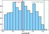 |
Fig. A.1. Redshift distribution of the selected sample. The red and green lines mark the redshift limits where the Hα and [O III] λ5007 lines start to fall outside the observed spectral range. |
Figure A.1 shows that the redshift distribution remains approximately uniform between z ∼ 0.1 and z ∼ 0.7, with fluctuations consistent with Poisson noise. Key emission lines used for EELG selection, such as Hα and [O III] λ5007, shift out of the J-PAS spectral coverage at z ∼ 0.4 and z ∼ 0.7, respectively. However, no significant decrease in source counts is observed at these redshifts. The number of detections only shows a noticeable decline beyond z ∼ 0.7, which is mainly driven by the increasing luminosity threshold imposed by our signal-to-noise cuts and the decreasing survey sensitivity at higher redshifts. Additionally, the increase in comoving volume with redshift helps maintain a relatively flat distribution up to this point. We also explored the distribution of absolute magnitude as a function of redshift (Fig. A.2). The plot illustrate the well-known Malmquist bias: at higher redshift, the sample becomes increasingly biased towards intrinsically brighter galaxies, since fainter sources fall below the survey’s detection limit. This effect is typical in flux-limited samples and must be considered when analysing the physical properties and number densities of EELGs across redshift.
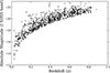 |
Fig. A.2. Distribution of galaxies in absolute magnitude in the SDSS i-band as a function of redshift. |
Appendix B: Neural network architecture details
This appendix provides a detailed description of the NN architecture used in the models. The structure consists of three parallel branches, each designed to process a distinct type of input: 1D photometric spectra, full-frame 2D galaxy images, and a localized image region centred on the galaxy’s emission line, intended to identify potential cosmetic artefacts. The individual layers used in this model are summarized in Table B.1.
B.1. Photometric branch
This branch handles 1D vectors representing the galaxy’s photometric fluxes across multiple bands. It begins with a 1D convolutional layer, Conv1D(64, 3), which scans along the spectral sequence to detect local patterns in the flux distribution. A MaxPooling1D(2) layer follows, which down-samples the signal to reduce dimensionality while preserving important features. A second convolutional layer, Conv1D(64, 3), captures more abstract spectral patterns. The output is then flattened and passed through a sequence of dense (fully connected) layers: Dense(128), followed by Dropout(0.3) for regularization, and two smaller layers with 64 and 32 units. These layers help the model combine and transform spectral information into a compact feature representation.
B.2. Image branch
The image branch processes a 2D cutout of the galaxy. It starts with a convolutional layer, Conv2D(64, 3 × 3), which extracts spatial features from the image. A MaxPooling2D(2 × 2) layer then reduces the spatial resolution. A second convolutional layer, Conv2D(32, 3 × 3), refines these features, followed by another MaxPooling2D. The resulting feature maps are flattened and passed through Dense(128) and Dropout(0.3), then through Dense(64), another Dropout(0.3), and finally Dense(32). This branch is primarily responsible for capturing the galaxy’s morphology – such as its compactness, elongation, symmetry, and surface brightness profile.
B.3. Cosmetic branch
The cosmetic branch receives a small image patch centred on the region where the galaxy’s emission line is located. This focused view allows the model to identify local anomalies – such as cosmic rays, hot pixels, or detector defects – that may affect the spectral measurement. The structure consists of a Conv2D(64, 3 × 3) layer, followed by MaxPooling2D(2 × 2), a Flatten operation, and two fully connected layers: Dense(64), Dropout(0.3), and Dense(32).
B.4. Fusion and output layers
After the feature extraction in each branch, the outputs are concatenated into a single combined vector. This joint representation is passed through a stack of dense layers: Dense(128), Dropout(0.3), Dense(64), Dense(32), and Dense(16). These layers allow the model to integrate the information from different inputs and produce the final prediction through the output node.
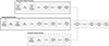 |
Fig. B.1. Model architecture consisting of three parallel branches designed for multi-mode data integration: (1) a spectral branch (upper), which processes the photometric flux through 1D convolutional layers; (2) an image branch (middle), which analyses the galaxy image using 2D convolutions to extract morphological features; and (3) a defect-detection branch (lower), which processes localized image regions around the emission-line position to identify cosmetic artefacts. Each branch applies a combination of convolutional, pooling, and dense layers, with dropout regularization to prevent overfitting. The outputs from the active branches are concatenated and passed through a shared set of fully connected layers, followed by a final sigmoid activation that produces the output label. For the primary EELG classifier (P0), only the spectral and image branches (upper and middle) are used. For the cosmetic-defect classifier (P1), all three branches are active, including the additional defect-detection branch. A detailed description can be found in Appendix B. |
NN layers and their role in the model architecture.
B.5. Overtraining
Given the relatively small size of the training dataset and the complexity of the NN, overfitting was a major concern. To mitigate this, we employed several strategies. First, the dataset was split into distinct training and test subsets, ensuring the model was evaluated on unseen data. Second, dropout layers with a rate of 30% were applied extensively throughout the network, effectively reducing co-adaptation between neurons and improving generalization. Third, early stopping was implemented based on the validation loss, stopping training once no further improvement was observed.
The learning curves for both training and test loss exhibit a consistent and monotonic decrease without the divergence typically associated with overfitting. This behaviour suggests that the chosen regularization strategies, particularly the dropout layers, are successfully preventing the model from memorizing the training data while maintaining strong predictive performance.
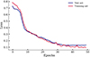 |
Fig. B.2. Test loss (blue) and training loss (red) as a function of training epochs. Both decrease monotonically without signs of overfitting. |
 |
Fig. B.3. Confusion matrix illustrating balanced prediction rates for true positives, true negatives, false positives, and false negatives. They all have similar occurrence rates, indicating a well-calibrated classifier without bias towards any class. |
B.6. Confusion matrix analysis
The confusion matrix provides a detailed breakdown of the classification performance by showing the counts or percentages of true positives, true negatives, false positives, and false negatives. In this particular case, the matrix reveals that the model predicts each of these outcomes with the same percentage. This balance indicates that the classifier does not favour any particular class and treats positive and negative predictions with similar accuracy. Specifically, the true positives and true negatives show that the model correctly identifies positive and negative cases at similar rates. At the same time, the false positives and false negatives, which represent the model’s errors in classification, also occur with comparable frequency. This symmetric distribution suggests that the model’s decision boundary is well calibrated and does not introduce significant bias towards one class.
Appendix C: CIGALE parameters
CIGALE parameters.
All Tables
All Figures
|
Fig. 1. J-PAS IDR202406 observed footprint with all the filters showing the positions of the seed fields. The coordinates (RA, Dec.) in degrees are: CODEX (126.1125, 40.1053), miniJPAS (214.4500, 52.7261), JPSV (244.00, 43.00), and StephQuint (339.00, 22.50). |
| In the text | |
|
Fig. 2. Data products from J-PAS for the EELG candidates. Left: J-PAS photometric spectrum (black line) and the corresponding DESI spectrum (red line). The shaded grey region marks the wavelength range selected for integration. Right: Image cutouts resulting from integrating the data cube over the selected spectral region. The horizontal white bar is 2 arcseconds in length. With J-PAS we are able to detect the continuum, but not with DESI. |
| In the text | |
|
Fig. 3. BPT diagram (Baldwin et al. 1981). Blue points are data points that have a counterpart in DESI with the Hα. The data points classified as AGNs are plotted in orange. The solid red line corresponds to the Kewley relationship (Kewley et al. 2001). |
| In the text | |
|
Fig. 4. 1:1 correlation observed between the spectroscopic redshifts and the best-fit values from LePhare. The inset quantifies the relative differences between the two redshift estimates. |
| In the text | |
|
Fig. 5. MS of star-forming galaxies. The plot shows the logarithm of the SFR, log(SFR10), versus the logarithm of the stellar mass, log(M★). The SFR10 refers to the average SFR over the past 10 Myr. Red points indicate galaxies with spectroscopic observations from DESI. The dotted black line shows the relation from Cole et al. (2025) at redshift 4.5–5. The solid black line corresponds to the relation from Curtis-Lake et al. 2021 (mock photometric samples of galaxies at z ≈ 5), the dot-dashed line the relation from Speagle et al. (2014), 64 measurements of the star-forming ‘MS’ from literature out to z ≈ 6), and the pink line the results from the Millennium Simulation (Springel et al. 2005). The dashed lines draw regions of constant sSFRs at values of −7 and −9. |
| In the text | |
|
Fig. 6. Histogram of the SFR10, sSFR10, stellar mass (M⊙), and extinction (E(B − V) for the J-PAS sample and its DESI counterparts. Vertical dashed lines indicate the mean values of each distribution. |
| In the text | |
|
Fig. 7. Photometric fluxes compared with the spectroscopic fluxes from the DESI counterpart for Hβ, Hα, and [O III] 5007 Å (from top to bottom). Grey lines indicate de limits of the ±1σ region. The red line represents the 1:1 ratio. |
| In the text | |
|
Fig. 8. Contour plot of the EWs of Hα and Hβ. Red histograms show the individual distributions along each axis. The contours represent the density of sources in the EW(Hα)–EW(Hβ) plane. Percentage shows the accumulative distribution and the grey line the 1:1 correlation. |
| In the text | |
|
Fig. 9. J-PAS EW compared with the spectroscopic EW from the DESI counterpart for [O III] λ5007 Å line emission. White triangles are upper limits. Grey lines indicate the limits of the ±1σ region. |
| In the text | |
|
Fig. 10. Relation between the ionizing photon production efficiency, log(ξion), and the rest-frame EW of [O III], log(EW0 [O III]). The blue points represent our sample of EELGs, with a typical error bar shown in the lower right region. The solid red line indicates the best-fit linear relation obtained in this work using a Markov chain Monte Carlo approach, with the shaded area showing the 1σ confidence interval. For comparison, previous relations from the literature are also shown: Tang et al. (2019), dashed), Pahl et al. (2025), dotted), Simmonds et al. (2024), dash-dotted), Llerena et al. (2024b), solid), and Begley et al. (2025), solid with dot.) |
| In the text | |
|
Fig. 11. Relation between the ionizing photon production efficiency, log(ξion), and the rest-frame EW of Hβ, log[EW0(Hβ)]. The blue points represent our sample. The shaded grey region marks the commonly adopted threshold (log(ξion) > 25.3). |
| In the text | |
|
Fig. A.1. Redshift distribution of the selected sample. The red and green lines mark the redshift limits where the Hα and [O III] λ5007 lines start to fall outside the observed spectral range. |
| In the text | |
|
Fig. A.2. Distribution of galaxies in absolute magnitude in the SDSS i-band as a function of redshift. |
| In the text | |
|
Fig. B.1. Model architecture consisting of three parallel branches designed for multi-mode data integration: (1) a spectral branch (upper), which processes the photometric flux through 1D convolutional layers; (2) an image branch (middle), which analyses the galaxy image using 2D convolutions to extract morphological features; and (3) a defect-detection branch (lower), which processes localized image regions around the emission-line position to identify cosmetic artefacts. Each branch applies a combination of convolutional, pooling, and dense layers, with dropout regularization to prevent overfitting. The outputs from the active branches are concatenated and passed through a shared set of fully connected layers, followed by a final sigmoid activation that produces the output label. For the primary EELG classifier (P0), only the spectral and image branches (upper and middle) are used. For the cosmetic-defect classifier (P1), all three branches are active, including the additional defect-detection branch. A detailed description can be found in Appendix B. |
| In the text | |
|
Fig. B.2. Test loss (blue) and training loss (red) as a function of training epochs. Both decrease monotonically without signs of overfitting. |
| In the text | |
|
Fig. B.3. Confusion matrix illustrating balanced prediction rates for true positives, true negatives, false positives, and false negatives. They all have similar occurrence rates, indicating a well-calibrated classifier without bias towards any class. |
| In the text | |
Current usage metrics show cumulative count of Article Views (full-text article views including HTML views, PDF and ePub downloads, according to the available data) and Abstracts Views on Vision4Press platform.
Data correspond to usage on the plateform after 2015. The current usage metrics is available 48-96 hours after online publication and is updated daily on week days.
Initial download of the metrics may take a while.