| Issue |
A&A
Volume 706, February 2026
|
|
|---|---|---|
| Article Number | A205 | |
| Number of page(s) | 12 | |
| Section | Planets, planetary systems, and small bodies | |
| DOI | https://doi.org/10.1051/0004-6361/202557463 | |
| Published online | 13 February 2026 | |
The vertical profile of the northern Io footprint auroral emission in the far-ultraviolet from Juno
Variability and energy spectrum of the precipitating electrons
1
Laboratory for Planetary and Atmospheric Physics, Space Sciences, Technologies and Astrophysical Research Institute, University of Liège,
Liège,
Belgium
2
Institute for Space Astrophysics and Planetology, National Institute for Astrophysics (INAF-IAPS),
Rome,
Italy
3
Department of Astrophysical Sciences, Princeton University,
Princeton,
NJ,
USA
4
Aix-Marseille Université, CNRS, CNES, Institut Origines, LAM,
Marseille,
France
5
Space Science Division, Southwest Research Institute,
San Antonio,
TX,
USA
★ Corresponding author: This email address is being protected from spambots. You need JavaScript enabled to view it.
Received:
29
September
2025
Accepted:
10
December
2025
Abstract
Context. The interaction between Io and the Jovian magnetosphere produces the auroral “Io footprint”, which can be observed in the ultraviolet thanks to the deexcitation of atmospheric H and H2 under electron precipitation. Since 2016, Jupiter has been explored with Juno’s Ultraviolet Spectrograph, which monitors the emission from 68 to 210 nm.
Aims. We used Juno observations of the Io footprint near the planetary limb to determine its vertical ultraviolet emission profile in the northern hemisphere. We simulated emission as a function of the altitude and the mean energy of the precipitating electrons, and we used the results to determine the energy spectrum associated with the footprint profile.
Methods. We estimated the source location of the Io footprint UV emission, and we extracted its vertical profile. We analyzed the variability of the emission altitude, and we derived the corresponding energy spectrum of precipitating electrons using TransPlanet. The results were compared with the in situ measurements from Juno’s particle detectors.
Results. The main spot emission peaks around ~500 km, with a variability of ~200 km correlated with longitude. The emission of the footprint tail within 20° from the main spot peaks around ~500±300 km, and it is moderately correlated with the magnitude of the magnetic field near Jupiter. The trans-hemispheric electron beam spot is located at ~300 km, and the associated precipitation appears depleted at low energy. The retrieved energy spectrum of the precipitation shows remarkable agreement with the particle measurements.
Conclusions. The longitudinal modulation of the Io footprint altitude suggests that the morphology of the torus affects the transmission of the Alfvén waves responsible for the acceleration of auroral electrons. The dependency of the footprint tail altitude on the magnetic field strength indicates that the magnetic field also plays a role in the acceleration mechanism.
Key words: plasmas / planets and satellites: aurorae / planets and satellites: gaseous planets / planets and satellites: magnetic fields
© The Authors 2026
 Open Access article, published by EDP Sciences, under the terms of the Creative Commons Attribution License (https://creativecommons.org/licenses/by/4.0), which permits unrestricted use, distribution, and reproduction in any medium, provided the original work is properly cited.
This article is published in open access under the Subscribe to Open model. This email address is being protected from spambots. You need JavaScript enabled to view it. to support open access publication.
1 Introduction
Jupiter's polar regions are constantly illuminated by powerful auroras, which can be detected over a wide range of wavelengths, from radio frequencies to X-ray (Drossart et al. 1989; Gladstone et al. 2002, 2007; Grodent 2015; Kurth et al. 2017; Trafton et al. 1989). The aurora is just one piece of evidence of the magnetosphere-ionosphere-thermosphere (MIT) coupling that deposits large amounts of energy into the polar regions of Jupiter (O'Donoghue et al. 2021; Roberts et al. 2025), where it affects the structure and composition of the atmosphere (Sinclair et al. 2020, 2023). Among the various auroral features, the orbital motion of the Galilean moons Io, Europa, Ganymede, and Callisto produces specific auroral emissions, called “footprints” (Connerney et al. 1993; Prangé et al. 1996; Clarke et al. 2002; Rabia et al. 2025). The moons orbit Jupiter slower than the magnetospheric plasma, which is “forced” toward rigid corotation with the planet by the MIT coupling currents. The moons act as obstacles to the plasma flow and produce a local perturbation, which propagates mainly as Alfvén waves along the magnetic field (Acuña et al. 1981; Belcher et al. 1981; Neubauer 1980). These waves accelerate particles along the magnetic field, producing electron precipitation into the planetary atmosphere (Damiano et al. 2019; Hess et al. 2010; Jones & Su 2008; Sulaiman et al. 2020). This process is particularly effective in the “acceleration region” ∼1-2 RJ above Jupiter’s surface1. Jupiter’s upper atmospheric layer mainly consists of H and H2 (Atreya et al. 2003), which are excited by the collisions with the precipitating magnetospheric electrons. The deexcitation of the hydrogen produces intense Lyman-α and Lyman and Werner bands, resulting in a strong extreme- and far-ultraviolet (EUV and FUV, respectively) aurora (Badman et al. 2015; Yung et al. 1982), which is partly absorbed by the hydrocarbons of Jupiter’s atmosphere.
The Io footprint (IFP) shows an ever-changing morphology that is governed by the pattern of the Alvén wavefront, known as “Alfvén wings”. The most evident feature is a bright spot at the foot of the main Alfvén wing originating at Io, which is thus called the “main Alfvén wing” (MAW) spot. Secondary spots associated with the reflection of the Alfvén waves, the “reflected Alfvén wing” (RAW) spots, and with the electrons accelerated at the opposite hemisphere, the “trans-hemispheric electron beam” (TEB) spots, are also consistently observed (Bonfond et al. 2008). Downstream of the MAW spot (with respect to the magnetospheric flow), the RAW spots are superimposed on an extended “tail”, which can encircle the entire polar region in the case of Io (Bonfond et al. 2017). The tail exhibits two smallscale substructures: “splits”. which are bifurcations of the tail in parallel arcs (Mura et al. 2018; Szalay et al. 2018), and “subdots”, which are regularly spaced patches of emission left behind the MAW spot along the tail (Moirano et al. 2021). To avoid any confusion within this complex morphology, we reserve the word “footprint” and “IFP” to generally refer to all the emissions observed at the feet of the magnetic shell crossing Io’s orbit, while we use “MAW spot” for the emission at the foot of the main Alfvén wing. We use “footprint tail” or “tail” to refer to all the emissions occurring downstream of the MAW spot (with respect to the magnetospheric flow past Io).
Juno is a spin-stabilized spacecraft that orbits Jupiter in highly eccentric polar orbits, and it has been observing the polar regions of Jupiter since 2016 (Bolton et al. 2017). Fig. 1 shows a sketch of the spacecraft trajectory near Jupiter. At the beginning of the mission, Juno reached its perijove (PJ, which is used to mark each orbit of the spacecraft) every ∼54 days, but this is now reduced to ∼32 days. The precession of the semi-major axis of Juno’s elliptic orbit increases the latitude of the perijoves and brings the spacecraft closer and closer to the northern hemisphere at each successive closest approach. Such orbital evolution creates favorable conditions to observe the aurora near the planetary limb, where it is possible to analyze the vertical profile of the emission. Juno spins with a period of ∼30 s, and it is equipped with an Ultraviolet Spectrograph (UVS; Gladstone et al. 2017b), which scans around the spacecraft as it spins and detects UV emission between 68 and 210 nm. This range includes Lyman lines of the atomic hydrogen, Lyman and Werner bands of the molecular hydrogen, and absorption bands by hydrocarbons such as methane, acetylene, ethylene, and ethane. The vantage point offered by Juno’s trajectory allows us to inspect the vertical distribution of UV emission of the IFP and therefore to derive information on the electron precipitation associated with the Io-Jupiter electromagnetic interaction.
In this work, we analyze Juno-UVS observations of the IFP acquired near the planetary limb from 2016 to 2025, corresponding to nearly 70 Juno orbits. We focus on the vertical profile of the FUV emission, which is determined by the energy spectrum of the electron precipitation and the atmospheric structure. To this end, we modeled the predicted location of the IFP emission as a 2D “curtain” located along the IFP track and the magnetic field, and we projected Juno-UVS observations on this surface in order to derive the vertical emission profiles associated with the footprint (see Fig. 1). In the present study we take full advantage of the well-known location of the IFP track, which allowed us to precisely locate the source of the emission, and the isolation of the footprint from other auroral features that may contaminate the analysis. The TransPlanet emission model (Benmahi et al. 2024a) was used to determine the electron precipitation corresponding to the observed emission and a given atmospheric structure. The results were compared with the data gathered by the particle detector of the Jovian Auroral Distributions Experiment (JADE; McComas et al. 2017), which crossed Io’s magnetic shell at least twice during each orbit and reported data near the main Alfvén wing in some occasions (Szalay et al. 2020b).
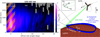 |
Fig. 1 Example of the typical observation geometry used to inspect the vertical profile of the IFP using Juno-UVS on February 22, 2022, corresponding to Juno’s 40th perijove. On the right, the blue ribbon represents the Io curtain, which is a 2D approximation of the source location of the auroral emission. Details on the IFP curtain are given in Sect. 3.1. Juno flies north-to-south along the dashed line while spinning around its spin axis. The green lines show the projection of the dog-bone shaped slit at 01:28:37.200 UTC. The xyz axes show the coordinate system of the Io curtain: x is along the IFP tail, z is along the magnetic field, and y is orthogonal to x and z, pointing poleward. The inset panel at the top of the right image shows the definitions of the angles used to select the observations at limb: α is the “heading angle” with respect to the direction of the IFP in Jupiter’s frame, β is the “pitch angle” with respect to the magnetic field, and γ is the “emission angle” with respect to the normal to the Io curtain. The left panel shows the vertical emission profile of the IFP in the 155-162 nm band, acquired between 01:21:35 and 01:44:15 UTC, as a function of the Alfvén-tail angle and altitude. The orange hatched area highlights the emission we excluded for the retrieval of the energy distribution of the precipitating electrons, as the instrumental pulse height distribution suggests an unreliable UVS calibration (only when using the wide slit). |
2 Observations and data reduction
The Juno-UVS observations of the IFP from PJ 1 to PJ 69 (from August 2016 to January 2025) are the backbone of the present analysis. The main components of UVS are the telescope, the slit, the scan mirror, and the detector (Gladstone et al. 2017a). The telescope is a Rowland circle spectrograph with a spectral bandpass at 68-210 nm. The light that passes through the telescope is focused through a dog-bone-shaped slit: the central part - the “narrow slit” - has a field of view (FOV) of 0.025×2 degrees, while the FOV of the sides - the “wide slits” -is 0.2×2.55 degrees. The spectral resolution varies between 0.4 and 1.1 nm across the detector (Gladstone et al. 2017b), and this is sufficient to identify groups of hydrogen lines, although not enough to resolve most of the individual fine-structure lines. It is worth noting that the width of each wide slit translates approximately into a tenfold increase in sensitivity with respect to the narrow slit; hence, the corresponding observed spectra have a signal-to-noise ratio (S/N) that is about ten times better. A scan mirror located at the front end of the telescope can be adjusted to point UVS between −30.2 degrees and 27.1 degrees from Juno’s spin plane. The detector is made of 2048 spectral pixels and 256 spatial pixels, although the active area is ∼1500×230 pixels. The narrow slit maps to the pixels between 119 and 169, while the two wide slit sides map to the pixels at 54-118 and 170-234.
The Juno-UVS dataset consists of lists of time-tagged events, which ideally correspond to all the UV photons that the instrument detects. In practice, a high-energy electron associated with the strong radiations within Jupiter’s magnetosphere can trigger a detection, which produces a spurious time-tagged event. From an instrumental point of view, the electron-triggered event is indistinguishable from a photon detection, but contrary to photons, the electrons are not diffracted by Juno-UVS optics, and hence their associated events are homogeneously distributed on the detector. For each PJ, we analyzed the EUV data of UVS -which has a very low sensitivity due to the instrumental counting efficiency falling sharply at short wavelengths - to estimate the radiation level (that is, the amount of events triggered by electrons), and we removed this background noise from the rest of the dataset. To this end, we took advantage of the low sensitivity of the detector between pixel 345 and 550 in the spectral dimension (∼60-81 nm) and between 20 and 255 in the spatial dimension to estimate the count rate due to radiation. This noise was then removed from the FUV-sensitive part of the detector. After removing the radiation-induced signal, we selected the events recorded when UVS was pointing at Jupiter within 2 degrees from the footprint of the magnetic shell intercepting lo’s orbit in order to restrict our analysis to the IFP. We also accounted for two instrumental parameters: the operational voltage and the pulse height. The voltage controls the instrumental gain, and it automatically adjusts to prevent strong bursts of radiation from damaging the detector. As the instrument is calibrated only for nominal voltage operations, we removed the events recorded at non-nominal voltage. The pulse height measures the height of the electronic pulses generated by the detector (Gladstone et al. 2017a; Hue et al. 2019, 2021) and was used to infer the performance of the instrument. We underline that this sanity check was carried out in retrospect, as it required us to inspect the pulse height distribution, which is computed from stacking together the individual pulse heights of a subset of events selected a posteriori based on their wavelength, time, and location. Therefore, the events used in images and spectra presented in this study were used to retrospectively produce the corresponding pulse height distribution. A reliable batch of events produced a unimodal pulse height distribution similar to a slightly skewed Gaussian distribution with an expected value greater or equal to five, while a smaller value suggests a gain loss. The threshold value was obtained by inspecting the spectral response of the detector for different pulse height distributions during the calibration sequences that UVS periodically performs. We remark that in any case, the brightness remains monotonically related to the count rate of the events. Consequently, the UVS data can still be used to accurately determine the location of a brightness maximum on an image, even when its absolute value is underestimated. From this retrospective analysis, the events corresponding to observations of the MAW spot performed with the wide slit consistently exhibited a pulse height distribution with an expected value below five; therefore, we used those events only to retrieve the location of the peak of the emission and not the energy spectrum of the precipitation. In the end, after the analysis of the pulse height distribution, the calibrated data we retained are the emission from the IFP tail using the wide slit (11 cases, corresponding to PJ 12, 31, 32, 33, 34, 40, 42, 44, 46, 50 and 59) and the emission from the MAW spot using the narrow slit (two cases, PJ 12 and 40). All of these cases were observed in the northern hemisphere. Due to the southward precession of Juno’s elliptical orbit, the instrument vantage point allowed us to observe the IFP vertical profile in the southern hemisphere with an acceptable S/N only in very limited time windows during PJ 3 and 8. During those orbits, Juno was much farther away from Jupiter than during the observations in the northern hemisphere, thus producing a degradation of the spatial resolution by a factor of about two to three, which makes the instrumental spatial resolution similar to the size of the IFP. For these reasons, this work focuses only on the IFP observations performed in the northern auroral regions.
3 Methods
In order to derive the characteristics of the precipitating electron associated with the IFP, we proceeded in two steps. First, we projected Juno-UVS observations onto the theoretical Io curtain and computed the column emission rate (hereafter “brightness”) of the IFP. We then extracted the vertical profile of the emission and used the TransPlanet code (Benmahi et al. 2024a) to simulate the UV volume emission rate (VER) as a function of the energy of the electron precipitation. This allowed us to retrieve the energy spectrum of the auroral electrons from the FUV vertical profile of the IFP.
3.1 Far-ultraviolet brightness of the Io footprint
To locate the source of the IFP emission and project UVS observations, we computed the theoretical Io curtain, which is a 2D approximation of the region where the IFP is observed. This surface corresponds to the surface containing the magnetic field lines intercepting the auroral IFP track between the 1-bar level (0 km) and 2000 km above. The footprint track was determined with the infrared observations of the Jovian Infrared Auroral Mapper onboard Juno (JIRAM; Adriani et al. 2017), which acquired infrared images within a few tens of minutes around the time of UVS acquisitions, depending on the observational constraints of the two instruments. The comparison between the statistical IFP track derived from JIRAM (Moirano et al. 2024) and that from UVS (Hue et al. 2023) over the period 20162022 showed remarkable agreement and negligible transversal variations over time. The magnetic field was computed with the Juno reference magnetic field (JRM33) model using the spherical harmonic expansion of the 18th order (Connerney et al. 2022) and the external magnetic field generated by the plasma disk that approximately extends from Io’s orbit at 5.9 R J (1R J = 71492 km is the equatorial radius of Jupiter) up to ∼50 Rj (Connerney et al. 2020). We used the freely available community codes (Wilson et al. 2023) and a Runge-Kutta fourth-order scheme to numerically compute the magnetic field lines passing through the IFP track. The sampling along each magnetic field line was 35 km, and the feet of the lines are 35 km apart. The curtain was thus represented by an approximately uniform grid with an average spatial resolution of ∼50 km. For the narrower FOV of the narrow slit, we increased the spatial resolution of the curtain by a factor of five, from ∼50 km to ∼10 km. This high-resolution grid was not used for the wide and the narrow slits, as it involves a much longer computational time, and it does not produce a better quality projection for the wide slit in terms of spatial resolution. For each grid point on the Io curtain, we defined three vectors (see panel in Fig. 1): a longitudinal vector along the footprint tail in Jupiter’s frame of reference (heading vector x), a nearly vertical vector aligned with the magnetic field and pointing outward from Jupiter (pitch vector z), and a vector normal to the Io curtain, obtained from the cross-product of the other two vectors (emission vector y). We used the angle between these three vectors and the UVS line of sight to compute the heading angle, α; the pitch angle, ß; and the emission angle, γ, respectively. These angles were used to select the UVS events when the emission was observed from the side. To this end, we selected events with a pitch angle, β, larger than 60 degrees and a heading angle, α, between 30 and 150 degrees. NASA’s Navigation and Ancillary Information Facility (Acton 1996; Acton et al. 2018, NAIF) provides the pointing vectors of the corners of the slit (eight for the two wide slit sides and four for the narrow slit, giving the vertices of a polygonal a dog-bone shape), but not for each pixel. The wide slits subtend 65 spatial pixels each, while the narrow slit subtends 51 pixels. Therefore, we divided the FOV defined by the pointing vectors of each slit by the number of spatial pixels behind that slit, obtaining an approximate FOV for each pixel (pixel-FOV). For each event recorded by UVS at a given time, the projection of the pixel-FOV onto the Io curtain identifies the source region of that event. The brightness of that event was computed according to the formula
 (1)
(1)
where W(λ) are the weighted counts in photons per square meter at a given wavelength, λ; texp is the exposure time in seconds; and γ is the emission angle as defined in Fig. 1. The resulting brightness was measured in Rayleigh (1 R = 1010 photons m−2 s−1; this photon flux is radiated in 4π steradians and includes the photons with a wavelength of λ ± ∆λ, where ∆λ is the spectral resolution). The weighted counts represent the conversion from the number of photons detected by the instrument to the actual number of photons, accounting for the counting efficiency of the detector (Greathouse et al. 2013; Hue et al. 2019). The exposure time is the time UVS observed a specific area. In general, this is not constant nor uniform across the detector, as the scan mirror skews the FOV on a given point on the sky and makes the exposure time uneven across the slit. In our study, the exposure time is computed as
 (2)
(2)
where Ωjuno is Juno’s angular frequency, 0.2 degrees is the aperture of the slit, and S is a shape factor that accounts for the position of the scan mirror (Gladstone et al. 2017b). For reference, the exposure time with the scan mirror in the default position (0 degrees from Juno’s spin plane) is ∼17 ms, and it reaches ∼34 ms at the extreme positions. For each event, we computed the brightness using Eq. (1), the geometry of the line of sight with UVS, the wavelength, and the Alfvén-tail angle, ∆λAlfvén (Szalay et al. 2020b). These values were assigned event by event to the grid points of the Io curtain. The Alfvén-tail angle was obtained by mapping the grid points of the Io curtain within the pixel-FOV at Io’s orbit along the magnetic field and taking the angular distance from Io at the time of the event. This distance must be corrected in order to account for the finite travel time of the Alfvén waves and its dependency on Io’s position within the Io torus (Szalay et al. 2020b). To this end, we used the average lead angle estimated from Juno observations (Hue et al. 2023; Moirano et al. 2024), which is proportional to the Alfvén travel time. The use of the Alfvén-tail angle as a metric is crucial to obtain images of the IFP with a high S/N. Indeed, the IFP moves at about 4 km/s in Jupiter’s frame; hence, it shifts by ~ 120 km from one Juno spin to another. The typical longitudinal size of the MAW spot is ∼400 km (Bonfond 2010; Moirano et al. 2024), and the hence spatial co-addition of events from successive spins leads to smearing, which in turn limits the S/N we can obtain by averaging multiple spins worth of data. Instead, the Alfvén-tail metric is approximately “anchored” to the longitude of the MAW spot; hence it allowed us to stack and average the observations of the IFP collected by UVS during multiple Juno spins, consistently increasing the S/N. We note that the RAW and TEB spots are not at fixed positions in this metric because they move relative to the MAW spot as Io orbits within the torus at different centrifugal latitudes. Nevertheless, those secondary spots do not move considerably over the time window when UVS can observe the IFP near the limb (approximately 0.5 degrees in ∼10 minutes). Although in principle we could average the IFP observations from multiple orbits, the location of the MAW spot is usually not the same across different orbits. Longitudinal differences are likely caused by the difference between the model lead angle used to compute the Alfvén-tail angle and the actual plasma conditions of the Io torus at each PJ (Moirano et al. 2023). Contrary to longitudinal variations, differences in altitude are instead ascribed to differences in the electron precipitation; they are thoroughly discussed in Sects. 4.1 and 5.1.
After all the events from a single PJ were projected, each grid point on the Io curtain contained the information collected over multiple Juno spins. For each of those spins, we reconstructed the IFP brightness by summing the brightness associated with all the events collected during that spin; in this way, we produced 2D images of the IFP projected onto the Io curtain, each corresponding to an individual spin of Juno. We interpolated the spin-by-spin projection and built four-dimensional hypercubes that contain the brightness of the IFP as a function of altitude (100 km sampling resolution), Alfvén-tail angle (0.2 degrees sampling resolution), wavelength (0.2 nm sampling resolution), and time (represented by Juno’s spin number). The spatial and spectral resolutions match approximately UVS specifications. These cubes can be easily averaged over several spins thanks to the use of the Alfvén-tail metric, producing spectral cubes with better S/N than a spin-by-spin analysis and without artifacts due to the IFP motion.
The UV spectrum of H2 is partially absorbed by hydrocarbons, especially at wavelengths <155 nm, while the solar illumination becomes non-negligible at >162 nm. In the 155162 nm band, C2H4 has the largest absorption cross section among the main hydrocarbons in Jupiter’s upper atmosphere. Nevertheless, in this study, we assumed that the 155-162 band is unabsorbed, as the low abundance of C2H4 (Sinclair et al. 2019) makes its absorption negligible above the 1-bar level (Gustin et al. 2013, 2016). From the hypercubes, we computed the average of the brightness over all Juno spins for each orbit, and we integrated between 155 nm and 162 nm, thus obtaining the IFP brightness as a function of altitude and Alfvén-tail angle (see the example in Fig. 1). We used TransPlanet to simulate the H2 spectrum between 80 and 170 nm produced by mono-energetic electron precipitations with energies between 0.5 and 10 keV, in agreement with the energy range of the particle measurements above the IFP (Szalay et al. 2020b), and we computed the ratio between the brightness in the 80-170 nm band and the 155162 nm band. The results show that this ratio varies between 0.140 and 0.142, and we thus divided the IFP brightness that we estimated from UVS data in the 155-162 nm band by 0.141 to obtain the total H2 UV brightness in the 80-170 nm band. The vertical profile of the total UV emission was then used to retrieve the energy distribution of the precipitating electrons, as explained in the next section.
3.2 Energy distribution of the precipitating electrons
The 2D projection of the IFP brightness was used to extract the vertical profile of the emission as a function of the altitude. We separated the profile into two regions, the MAW spot and the tail. The MAW spot is usually at an Alfvén-tail angle between −2 and 2 degrees and its longitudinal extension is <1 degree. The pulse height distribution associated with the MAW spot consistently exhibits an expected value below five in the wavelength range 125-165 nm when observed through the wide slit. This suggests that instrumental effects on this specific region cause a local loss of counting efficiency and render the calibration less reliable. Therefore, we derived the vertical profile of the tail between 3 and 10 degrees, and between 10 and 20 degrees by taking the average brightness over those ranges. Farther down the tail, the S/N becomes very low, and hence we limited our analysis between 3 and 20 degrees. The events recorded through the narrow slit show a good pulse height distribution when observing the MAW spot, so the brightness calibration is reliable. We therefore extracted the vertical profile of the MAW spot between −0.5 and 0.5 degrees for PJ 12 and 40.
TransPlanet uses a given atmospheric model and an input electron energy spectrum to produce the VER integrated between 80 and 170 nm as a function of the altitude and the energy of the precipitating electrons. In the present analysis, we adopted the auroral atmospheric model by Grodent et al. (2001); the model can use mono-energetic distributions with energies between 0.4 keV and a few hundred kiloelectronvolts as input. In general, precipitations at energies < 10 keV produce vertically broad emission that peak above 500 km, while precipitations at energy > 100 keV lead to deep emission below 300 km. Above ∼50 keV, the emission is confined within a thin layer of <100 km, which corresponds to the spatial resolution of the profile extracted from UVS observations. This emission peaks below ∼300 km, and thus we excluded the brightness profile below 300 km in order to properly compare the model VER with the observed brightness. Using TransPlanet, we first simulated the volume emission rates produced by mono-energetic electron precipitations with an energy flux of 1 mW m−2 at various energies, and we computed the total VER as the linear combination
 (3)
(3)
where Ei = 0.05, 0.1, 0.4, 1, 2, 4, 8, 16, 32 keV, and αi is a set of free parameters. Eq. (3) is valid in an optically thin medium, such as H2, at wavelengths >120 nm. The theoretical brightness, ITP, obtained from TransPlanet was computed by integrating the VER along the line of sight of UVS, assuming that no other source of emission is present along the line of sight. To perform the integration, we assumed that the cross section of the IFP can be approximated by a Gaussian function with a standard deviation, σT (Moirano et al. 2024):
 (4)
(4)
Here, y and z are the coordinates shown in Fig. 1, VER0 is the VER at the center of the footprint, and σT is the IFP cross section estimated by mapping Io’s cross section from its orbit onto Jupiter’s surface using the magnetic field model JRM33 to account for the effect of the magnetic field geometry on the transversal size of the IFP. The model brightness could then be computed as
 (5)
(5)
Using Eqs. (5) and (3), we obtained
 (6)
(6)
where VER0(Ei,z) is from TransPlanet. For a given energy, Ei, the VER is directly proportional to the energy flux, and therefore we could fit Eq. (6) to the vertical profile extracted from UVS data and retrieve the coefficients ai, which correspond to scaling factors for the energy flux at the energies Ei. As the volume emission rates on the right hand side of Eq. (3) are computed from mono-energetic electron spectra with an energy flux Φ =1 mW m−2 = 6.24·108 keV s−1 cm−2, the intensity of the precipitation at a given energy, Γ(Ei), corresponding to the IFP profile was computed using the coefficients ai :
 (7)
(7)
where ∆Ei is the width of the energy bins. Note that the intensity, Γ(Ei), is a particle flux per unit energy.
We used the Markov chain Monte Carlo algorithm by Haario et al. (2001, 2006) implemented in MATLAB (Laine 2020,2) to sample the distribution of the free parameters, ai, and we determined their values and uncertainties from the expected value and the standard deviation of the final distributions. Determining the convergence of a Markov chain is an active area of theoretical research, and only diagnostic tools are available (Cowles & Carlin 1996). In this study, we considered a small autocorrelation as an index of convergence. An example of the fit to the IFP profile is given in Fig. 2.
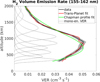 |
Fig. 2 Volume emission rate corresponding to the average brightness of the Io tail between 3 and 10 degrees, extracted from the observations during PJ 40 (see Fig. 1) using Eq. (5). The black solid line is the extracted profile with the associated uncertainty (gray area). The green line is the fit using a Chapman function Eq. (9) (Bonfond 2010), and the red line is the fit using the linear combination in Eq. (6) computed from TransPlanet. The thin black lines show the individual volume emission rates obtained from mono-energetic electron precipitations with an energy of 0.05, 0.1, 0.4, 1, 2, 4, 8, 16, and 32 keV (from high to low altitudes). The profile below 300 km was excluded, as the volume emission rates generated by precipitations with energy ≳50 keV peak below that altitude and undersample the profile at a spatial resolution of ~ 100 km. |
4 Results
We used the hypercubes generated by projecting the UVS events onto the modeled Io curtain to generate 2D plots of the IFP brightness and to compute the FUV spectra at each spatial point in the brightness profiles, such as the one in Fig. 1. The correctness of the projection on the Io curtain strongly relies on the position of the IFP track, and the transversal displacements of the IFP with respect to its reference track produce an incorrect altitude mapping. So far, the IFP has not shown any strong transversal displacement from its reference track over time (Moirano et al. 2024), and it does not appear to be correlated with the expansion and contraction of the main emission (Head et al. 2024). Instead, it has been used as a fixed reference for other auroral features (see, for example, Grodent et al. 2008). From the infrared images recorded by Juno-JIRAM at high spatial resolution (down to less than 10 km; Moirano et al. 2024), we considered the transversal size of the IFP (∼150 km) as the upper limit on the transversal displacement of the footprint, which corresponds to an angular uncertainty of ∼0.1 degrees in the IFP coordinates. This introduces an expected uncertainty due to parallax lower than 100 km, which is the spatial resolution achieved by UVS when looking at the IFP. As an additional self-consistency check, we computed the hydrocarbon color ratio (CR) using the FUV spectrum:
 (8)
(8)
where I(155-162) is the FUV brightness integrated between 155 and 162 nm, which we considered unabsorbed, and I(130-153) is the brightness integrated between 130 and 153 nm, where CH4, C2H2, and C2H6 are the main hydrocarbons responsible for absorption. We did not use data below 130 nm, as the pulse height distribution below this wavelength usually has a peak below 5, suggesting that the corresponding brightness is underestimated. We used the color ratio vertical profile to verify that the projection is consistent and not affected by parallax. Fig. 3 shows that the color ratio is indeed nearly uniform above 300 km, while it rapidly increases in the deepest layers, in agreement with previous studies (Yelle et al. 1996; Grodent et al. 2001; Moses et al. 2005; Sinclair et al. 2020; Sánchez-López et al. 2022; Migliorini et al. 2023; Mura et al. 2025). The color ratio enhancement below 300 km is consistent between all the Juno orbits that we considered, strongly suggesting that the altitude mapping we produced is accurate.
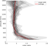 |
Fig. 3 Color ratio obtained from the vertical brightness profile of the IFP between 3 and 10 degrees with Eq. (8). The black lines are the orbit-by-orbit color ratios with their respective uncertainty (gray areas). The red solid curve is the average color ratio, and the red dashed lines are the 1σ boundary of its uncertainty. The data below 100 km were excluded due to poor S/N. |
4.1 Altitude profile
We used the vertical profile extracted from 11 selected Juno orbits to determine the emission peak altitude. To this end, we fit a Chapman function to the vertical profile (Bonfond 2010):
![Mathematical equation: C(z) = Aexp\Bigg[1-\frac{z-z_0}{L}-exp\Big(-\frac{z-z_0}{L}\Big)\Bigg]+B,](/articles/aa/full_html/2026/02/aa57463-25/aa57463-25-eq9.png) (9)
(9)
where A is the peak brightness, z0 is the altitude of the peak, L is the vertical extension of the emission, and B accounts for the emission background. For each fit, we computed the reduced  to assess the robustness of the results:
 (10)
(10)
where Rh and ∆h are the fit residuals and measurement uncertainty as a function of altitude, respectively, while ν represents the degrees of the freedom. The UVS photon counts follow a Poisson distribution, whose mean and variance are equal, and hence the measurement uncertainty was computed as
 (11)
(11)
where IUVS (h) is the measured brightness at altitude h (Eq. (1)), and Nh is the number of photon counts used to compute IUVS (h). For the 11 cases we analyzed,  was between 1.0 and 1.6.
Figure 4 shows the altitude of the emission peak obtained from the MAW spot profile as a function of MAW longitude and magnetic mirror ratio. In this work, we use westward longitude, which comes from the left-handed frame of reference known as “System III” (Seidelmann & Divine 1977). The peak altitude shows strong variability from one orbit to the other, with values between ∼250 km and ∼700 km, and an average of 493 km. The footprint tail exhibits a similar variability. In this case, the altitude lies between ∼400 km and ∼950 km, with an average of 589 km. The altitude was fit with a sinusoidal function of longitude, while for the mirror ratio, we used a linear regression model. For each fit, we used the adjusted coefficient of determination R to assess the quality of the fit (Ezekiel 1930):
 (12)
(12)
which estimates the fraction of the variation in the dependent variable predicted by the model. In the equation, n is the number of data points, p is the number of model parameters, SSE is the sum of squared residuals (or errors), and SST is the sum of squared total:
 (13)
(13)
where yi is the ith data point and  is the average of the yi. The term R
 accounts for the number of model parameters, and thus it allowed us to meaningfully compare the fits in Fig. 4. The fit as a function of the IFP longitude provided R
 =0.56 and 0.61 for the MAW and tail, respectively, while for the mirror ratio we obtained R
 =0.15 and 0.45. We also analyzed the altitude as a function of Io’s longitude and magnetic field magnitude at the surface (not shown), and they returned similar results to Fig. 4. This is not unexpected, as there is a one-to-one correspondence between Io’s longitude and the IFP longitude and between the surface magnetic field and the magnetic mirror ratio. Furthermore, we also verified a possible correlation with the magnetic dip angle, the IFP latitude, and the orbit number. These parameters appear to be irrelevant to the altitude of the emission. We computed the altitude difference between the MAW spot and the tail for each orbit. On average, the MAW spot occurs 130±110 km deeper than the tail. Seven cases out of the 11 analyzed show that the emission associated with the MAW spot is deeper by ∼100-270 km. We did not find significant correlation between the altitude difference and the position of the IFP or the magnetic field.
Lastly, we compared the altitude of the MAW spot with the altitude of the TEB spot. The TEB spot moves with respect to the MAW spot because of the evolution of Io’s magnetic latitude as it orbits Jupiter; hence, we selected the orbits when the TEB spot was upstream from the MAW spot in order to avoid the interplay between the TEB and the footprint tail. By analyzing PJs 12, 33, 42, and 46, we found that the TEB spot emission occurs at 100±88, 418±86, 342±52, and 299±44 km, respectively, deeper than the MAW spot by ∼300 km.
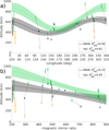 |
Fig. 4 Altitude of the peak emission of the MAW spot (black squares), the IFP tail (green diamonds), and the TEB spot (orange circles) as a function of longitude (panel a) and the magnetic mirror ratio (panel b). The double longitude labels indicate the footprint (top) and moon longitudes (bottom), respectively. The data points are obtained from Juno-UVS, and the error bars are 1σ. For the MAW spot data, the solid black lines are a sinusoidal fit in panel a and a linear fit in panels b, respectively. The green dashed lines are the same type of fit, but for the tail data. The thin black lines connecting MAW and TEB tail points link data from the same Juno orbit (note that the MAW spot around 360 degrees is associated with the TEB spot near 0 degrees). The gray, green, and orange bars attached to the y axis show the average altitude of the three features and their respective standard deviations. |
4.2 Retrieval of the energy spectrum of the precipitating electrons
The VER computed with TransPlanet is proportional to the intensity of the electron precipitation. Therefore the correct calibration of the FUV brightness is essential for a robust retrieval of the electron energy spectrum from UVS observations. For this reason, we excluded the observations of the MAW spot performed using the wide slit of UVS, as the corresponding pulse height distribution suggests that the MAW brightness is underestimated. We used the method explained in Sect. 3.2 to constrain the free parameters in Eq. (6), which are directly related to determining the intensity of the precipitation into the IFP through Eq. (7). The  returned values between 0.9 and 1.3, which supports the robustness of our results.
We used JADE data corresponding to the crossings of Io’s magnetic shell to compare them with our retrieved energy spectra, as the instrument measures the electron energy between 50 eV and 100 keV (Szalay et al. 2020a), which is the energy range that we investigated with TransPlanet. We selected JADE data acquired within 20 degrees from the MAW spot to directly compare them with the results retrieved from UVS data. We considered only the electron measurements below 1 RJ from Jupiter’s surface in order to sample the downward-going population that is accelerated by the moon-magnetosphere interaction. Indeed, the energy transfer from the Alfvén waves to the precipitating electrons is particularly efficient between approximately 1 and 2 RJ from the Jovian surface (Hess et al. 2010). Suitable JADE data are available for PJs 5, 12, 13, 22, 29, 40, 56, and 61. For each of these, we computed the average using the three most intense spectra measured by JADE, and they were compared with the retrieval based on the UV profile. Fig. 5 shows the energy spectrum obtained from the IFP tail observed during PJ 40 (the same data as in Figs. 1 and 2). JADE data were recorded at an Alfvén-tail angle of 10 degrees, and hence we compared those directly with the UVS retrieval obtained by averaging the IFP profile between 5 and 15 degrees. The comparison shows a remarkable similarity in the overlapping energy range, especially below 10 keV, above which JADE often did not make sufficient total count rates to fully resolve the intensity distribution above background levels within the IFP tail (Szalay et al. 2020b).
Panel a of Fig. 6 shows the electron energy spectrum measured by JADE during PJ 12, when Juno crossed the MAW connected to Io, and we compared it with the retrieved electron energy spectrum using UVS data from PJ 12 and PJ 40 acquired with the narrow slit. Thanks to the Alfvén-tail metric used to build the spectral hypercubes (see Section 3.1), we were able to increase the S/N by averaging the data acquired over approximately 20 Juno spins for each orbit. For orbits other than PJ 12 and PJ 40, UVS did not collect enough data to reconstruct the shape of the IFP with the narrow slit, as its smaller FOV also limits the spatial coverage. The comparison shows again a remarkable similarity. The spectrum retrieved from UVS data for PJ 12 exhibits a higher intensity than the JADE measurements, which may indicate that Juno flew very close but perhaps not through the peak of the precipitation associated with the MAW spot.
Panels a and b of Fig. 6 compare the UVS retrievals with the JADE data obtained from all Juno orbits considered in this work. The results are divided into two regions - between 3 and 10 degrees (which JADE covered during PJ 22, 29, and 40) and between 10 and 20 degrees (which JADE covered during PJ 5, 13, 56, and 61) - to highlight potential differences along the footprint tail. The UVS retrievals seem to slightly underestimate the measured energy spectrum between 1 and 10 keV, but overall the two instruments give consistent results in both regions. The UVS retrievals between 10 and 20 degrees show a larger uncertainty, which is caused by the decreasing S/N of the FUV brightness along the tail.
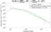 |
Fig. 5 Retrieval obtained from UVS data (solid black line) and JADE electron measurements (gray dotted line) during PJ 40. JADE data were acquired at an Alfvén tail angle of 10 degrees, while the vertical profile used in the retrieval was obtained by averaging the IFP brightness between 5 and 15 degrees. The green line is the linear fit to the UVS retrieval. |
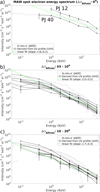 |
Fig. 6 Electron energy flux retrieved from UVS data (solid black lines) and JADE electron measurements (gray dotted lines). JADE data in panel a were acquired during the MAW crossing of PJ 12 (April 1, 2018), while the vertical profile used in the retrieval was obtained by averaging the MAW brightness of PJ 12 and PJ 40 (the latter occurred on February 25, 2022) between −0.5 and 0.5 degrees, using the data from the narrow slit of UVS. The green dashed line is the linear fit to the UVS retrievals. The retrievals with 1σ uncertainty larger than the retrieved intensity were omitted. Panel b shows a comparison among data collected between 3 and 10 degrees. Panel c shows a comparison among data between 10 and 20 degrees. |
5 Discussion
5.1 Variability of the IFP altitude
The altitude of the FUV auroral emission associated with the IFP shows noticeable variability, as shown by the 11 observations near the planetary limb by Juno reported in Fig. 4. The altitude of the IFP - both the MAW spot and the tail - shows a correlation with the longitude, while only the tail shows a moderate correlation with the magnetic mirror ratio, as suggested by the R retrieved from the sinusoidal and linear fits. The profile of the color ratio shown in Fig. 3 exhibits much smaller variations than the altitude of the IFP. Indeed, the color ratio starts to consistently increase at 300-400 km, while the emission peak altitude of the IFP lies between 250 and 700 km for the MAW spot and between 400 and 950 km for the tail. The upper limits of these values are consistent with the previous estimate of the emission peak altitude of the IFP tail based on Juno observations (Szalay et al. 2018). The difference between the variation in color ratio profiles and brightness profiles strongly suggests that the variability of the emission altitude is not a result of parallax. Hubble Space Telescope (HST) observations of the IFP collected between February and June 2007 observed the northern IFP mostly in the longitudinal sector between 120 and 260 degrees (Bonfond et al. 2009). The limited spatial coverage was caused by HST’s vantage point, which is challenging for observing the aurora near the pole, and the IFP track reaching latitudes above 80 degrees (Connerney et al. 2022). The analysis of the IFP near the planetary limb by Bonfond et al. (2009) showed that the altitude of the tail is nearly constant within the uncertainty, and it is located between 600 and 1100 km from the surface, with an average of ~900 km. These values are 200-300 km higher than the results shown in Sect. 4.1. The HST observations require the limb fitting of Jupiter, which depends on assumptions about the atmospheric structure, to determine the instrument pointing. Conversely, Juno’s position and orientation were retrieved from NASA’s NAIF database, which uses the onboard star tracker, and thus it was determined independently from UVS data. The different methods used may then be the root cause of the discrepancy. The increase of the color ratio in Fig. 3 at the expected location around 300-400 km supports the accuracy of the present analysis. Alternatively, the difference between the present results and those reported by Bonfond et al. (2009) might be caused by different conditions in the Io torus. Damiano et al. (2019) simulated the broadband electron acceleration generated by kinetic Alfvén waves at around 1.5 RJ, and they inspected the role of the density gradient between the plasma in the plasma disk or Io plasma torus and the high-latitude magnetosphere. They showed that the simulations with the Io plasma torus produce more energetic precipitation than simulations without strong density gradients and suggested that the high density of the Io plasma torus reduces the group velocity of the Alfvén waves, which in turn produce larger wave amplitudes. This ultimately leads to higher intensities at high energy. Therefore, we qualitatively inferred that a higher torus density produces an energy precipitation with a stronger intensity at high energy than a depleted torus. In turn, such precipitation penetrates deeper into the atmosphere, and thus the UV auroral emission is expected to peak at a lower altitude. Using the HST observations of the MAW spot between 2005 and 2007, Schlegel & Saur (2023) reported that the torus plasma density was ∼2000±400 cm−3, while Moirano et al. (2025) obtained a density of ∼3000±1400 cm−3 when using Juno observations from 2016 to 2022. Although the large uncertainties prevent us from drawing definitive conclusions, the observations of the IFP at a lower altitude with Juno compared to HST appear consistent with the higher plasma density in the Io torus in the period 2016-2022 compared with the 2005-2007 period.
Hess et al. (2011) suggested that the asymmetric magnetic field of Jupiter is responsible for longitudinal variations in the efficiency of the wave-particle interaction that accelerates the auroral electrons, as a stronger surface magnetic field (and thus a higher mirror ratio) is more efficient in producing high-energy electrons. The adjusted R of the linear regression of the MAW spot altitude as a function of the mirror ratio is 0.15, while we obtained R
 =0.45 for the tail. We also computed the Pearson correlation coefficient R (Press 2007) between the altitude of the emission and the mirror ratio for both regions, obtaining R= −0.5
 and −0.7
 , respectively. These values suggest that the magnetic field asymmetry could modulate the tail altitude by affecting the efficiency of wave-particle energy exchange and consequently the energization of the auroral electrons. Fig. 7 shows the correlation between the magnetic mirror ratio and the intensity at 0.1,0.4,1, 2,4, 8,16, and 32 keV shown in the middle panel of Fig. 6, i.e. for ∆λAlfvén from 3 to 10 degrees. For energies above 1 keV, we found a positive correlation within 1-2σ, which indicates that the larger the mirror ratios (that is, the stronger the field at the surface), the higher the intensity above 1 keV. For energies ≤1 keV, the correlation is negative, indicating that the particle flux at those energies is depleted in the regions with a strong magnetic field. In contrast, the correlation of the MAW spot altitude with the mirror ratio is uncertain, and hence the role of the magnetic field at the surface may be less relevant than for the tail.
The IFP longitude modulates the MAW spot altitude as much as the tail. The sinusoidal fit in panel (a) of Fig. 4 has a minimum at ∼150 degrees and a maximum at ~330. Io orbits within the Io plasma torus, a toroidal plasma cloud generated by the atmospheric loss from the moon itself (see, for example, the review by Bagenal & Dols 2020). The plasma distribution of the Io plasma torus is determined by the magnetic field geometry, the centrifugal force, and the internal plasma pressure. Consequently, the Io plasma torus is tilted by approximately 7 degrees from Jupiter’s equator, toward ∼200 degrees longitude in the System III frame of reference (Phipps et al. 2020). The Io plasma torus is asymmetric, showing a 5-20% increase in electron density around 160 degrees longitude and a depletion below 60 degrees and above 330 degrees (Steffl et al. 2006; Hess et al. 2011). The longitudinal variation of electron density is suggested to be ultimately driven by the presence of a hot electron population in the Io plasma torus, with a typical energy of ∼40 eV (Bagenal & Dols 2020), which in turn affects the Io plasma torus composition (Steffl et al. 2008). The Io plasma torus extends for ∼10 degrees in latitude, and the negative density gradient between the core of the Io plasma torus and the high-latitude magnetosphere likely affects the energization of the electrons (Damiano et al. 2019). The correlation of the IFP altitude with longitude and the similar trend between the IFP altitude and the Io plasma torus electron density suggest that the longitudinal modulation of the IFP altitude may be a consequence of the Io plasma torus morphology. The model by Damiano et al. (2019) is designed to mainly explore the physics and the parameters involved in the electron acceleration, and a quantitative comparison between their simulations and UVS observations will require the inclusion of the parameters specific to the Io case.
Based on the comparison of the MAW spot with the tail and their dependency on the IFP longitude and mirror ratio, we suggest that the vertical FUV profile of the MAW spot is mostly determined by the details of the plasma environment near Io, while the tail profile depends on both the plasma conditions at Io’s magnetic shell and the magnetic field geometry. Quantitatively comparing the Io plasma torus conditions with the UV emission profile would require simultaneous measurement of the Io plasma torus density and a moon-magnetosphere coupling model able to produce the energy spectrum of the precipitating electrons for various torus conditions in terms of density and temperature. These are not readily available in the literature3, and their development falls outside the goals of the present study. Ground-based monitoring of sodium and S+ at 589 and 673.1 nm from Jupiter’s inner magnetosphere was conducted between 2017 and 2023 (Morgenthaler et al. 2024), which, in principle, can provide the foundation for simultaneous comparison of the data and the results analyzed in the present study.
The color ratio shown in Fig. 3 shows an increasing hydrocarbon absorption in the 130-153 nm band below 300-400 km. The agreement with previous studies on the hydrocarbon vertical distribution (Grodent et al. 2001) and the consistency of the color ratio profile retrieved from UVS dataset demonstrate the robustness of the projection technique described in Sect. 3.1. The analysis of the color ratio profile to retrieve the hydrocarbon abundances is currently underway and will be addressed in a separate work.
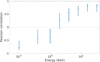 |
Fig. 7 Correlation between the magnetic mirror ratio and intensity for energies of 0.1, 0.4, 1, 2,4, 8, 16, and 32 keV obtained using the IFP tail profile (∆λAlfvén = 3-10 degrees). The error bars are 1σ. |
5.2 Energy of the electron precipitation
The energy spectra of the precipitating electrons retrieved from the FUV vertical profile in Fig. 6 are broadband, with the most intense flux usually below 1 keV. The presence of broadband spectra associated with the moon-magnetosphere interaction and the IFP is consistent with previous in situ field, particle, and wave measurements (Bonfond et al. 2009; Gershman et al. 2019; Sulaiman et al. 2020; Szalay et al. 2018, 2020b). The intensity we obtained from the tail profile exhibits variability within a factor of ten, which is consistent with the variability in the energy spectra measured by JADE.
By comparing the spectrum obtained from the MAW spot profile in panel a of Fig. 6 with the tail profile in panels b and c, we noticed that the MAW spot spectrum is flatter and about one order of magnitude more intense than the tail spectrum. The tail spectrum above ~1 keV is depleted compared to the MAW spectrum in both the UVS retrieval and JADE data. To quantitatively determine the difference between the two IFP regions, we computed the linear fit to the retrieved electron energy spectra (in the logarithmic scale) and compared the slopes. For the MAW spot in Fig. 6, we obtained −1.6±0.2, while for the tail in Fig. 6 we estimated −2.0±0.5 and −1.7±0.3 at different Alfvén-tail angles. These values agree with a previous estimate that used a powerlaw energy spectrum for the precipitation (Bonfond et al. 2009) and showed that the depletion of electrons above 1 keV occurs mainly from the MAW spot to the tail. The steepening of the profile toward the tail is consistent with the altitude of the profile. High-energy electrons penetrate deeper into the atmosphere, and hence the emission of the MAW spot peaks at a lower altitude, as shown in Sect. 4.1.
We used a kappa distribution (Coumans et al. 2002) to fit the electron energy spectra in Fig. 6 in order to retrieve the mean energy of the precipitation. The fitting function of the energy, E, is
 (14)
(14)
where Q0 is the total intensity, E0 is the energy corresponding to the maximum intensity (called “characteristic energy”), and κ is an index retrieved as a free parameter. The mean energy was obtained from the characteristic energy:
 (15)
(15)
From the fits to the 11 footprint tail profiles in panel b of Fig. 6, we obtained Q0 between 2.5∙109 and 1.6∙1010 cm−2 s−1 keV−1 sr−1, 〈E〉 between 0.4 and 3 keV, and κ between 2.3 and 2.6, values which are in agreement with previous analyses (Bonfond et al. 2009). This range of values indicates variability in the precipitation associated with the IFP within 1σ for the mean energy and the kappa index and within 2σ for the total intensity. From the vertical profile of the MAW spot of PJ 40, we obtained Q0 = 8±5∙1011 cm−2 s−1 keV−1 sr−1, 〈E〉 = 13±6 keV, and κ = 2.1 ±0.2, while for PJ 12 the fit did not produce significant results due to the large uncertainty on the retrieved parameters. The lower κ value in the MAW spot with respect to the tail is consistent with the lower slope of the power law fit in panel a of Fig. 6 compared to panel b and c. The intensity Q0 retrieved from the vertical profile of the MAW spot and the footprint tail is approximately two orders of magnitude greater than the precipitation associated with the main auroral emission of Jupiter (Szalay et al. 2017; Salveter et al. 2022), while the mean energy 〈E〉 associated with the IFP is one to two orders of magnitude lower than the mean energy of the main emission (Mauk et al. 2017, 2020; Benmahi et al. 2024b).
The emission of the TEB spot is usually located ∼300 km deeper than the MAW spot, peaking below 300-400 km. In Fig. 8, we compared the energy spectra retrieved from the MAW and TEB spots and the tail observed during PJ 12. The spectrum associated with the TEB is similar to that of the MAW spot, but with an intensity that is about three orders of magnitude smaller. The TEB and tail spectra have similar intensities overall (within one order of magnitude), although the TEB spectrum is flatter and exhibits a “shoulder” at ∼3 keV. The difference between the two regions is most notable below 10 keV, suggesting a depletion at low energy, rather than an enhancement at high energy; this consists with previous estimates (Hess et al. 2013).
Previous limb observations of the IFP reported that the TEB was located approximately 200 km below the MAW spot (Bonfond et al. 2009), which is consistent with our results.
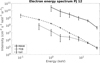 |
Fig. 8 Energy spectra retrieved from UVS data acquired during PJ 12 (April 1, 2018). The black solid curve was obtained from the MAW spot profile using the UVS narrow slit, while the dotted and dashed lines come from the TEB spot and the tail, respectively. |
6 Conclusions
We analyzed the FUV observations of the IFP performed by Juno from August 2016 to January 2025, which includes nearly 70 orbits of the spacecraft around Jupiter. We selected the data corresponding to when the footprint was near the planetary limb as observed by the UVS instrument in order to inspect the vertical profile of the H2 auroral emission generated by the electron precipitation associated with the moon-magnetosphere interaction. We used Juno high-resolution observations of the IFP recorded by Juno (Hue et al. 2023; Moirano et al. 2024) and the JRM33 magnetic field model (Connerney et al. 2022; Wilson et al. 2023) to precisely locate the source region of the emission and extract the vertical profile associated with various features of the footprint: the MAW and TEB spots and the tail. The profile was fit with the vertical profile of the emission rate modeled with TransPlanet (Benmahi et al. 2024a) in order to retrieve the energy spectrum of the precipitating electrons, which was compared with the particle measurement performed by JADE (Szalay et al. 2020b) corresponding to the various features of the IFP.
The altitude of the IFP emission shows significant variability: the peak emission of the MAW spot occurs mostly between 250 and 700 km, while the tail emission peaks between 400 and 950 km. These values are smaller than what has been reported based on HST observations (Bonfond et al. 2009; Bonfond 2010). A possible explanation for this discrepancy lies in the different methods used to determine the IFP position between HST and Juno-UVS (see Section 5.1). To verify the reliability of our analysis, we estimated the vertical profile of the hydrocarbon color ratio. This boundary is expected to be at around 300400 km, which is in agreement with our results in Fig. 3. The agreement between our results and JADE measurements serves as an additional retrospective validation, as the altitude of the emission depends on the energy spectrum of the precipitating electrons. Alternatively, the discrepancy may originate in the different torus conditions at different times. On one hand, Schlegel & Saur (2023) reported a torus density of ∼2000 cm−3 when using HST data from 2005 to 2007; in the same period, the IFP peak emission was detected at ∼900 km (Bonfond et al. 2009).
On the other hand, the torus density in the period 2016-2022 was estimated to be ~3000 cm−3, and the peak emission altitude of the IFP we retrieved in this study is ∼500-600 km. Qualitatively, we inferred from the model by Damiano et al. (2019) that a high plasma density in the Io torus produces a high-energy precipitation, which generates auroral emission that peaks at a low altitude. This appears to be consistent with the present and past observations of the UV vertical profile of the IFP, although a proper quantitative analysis will require ad hoc modeling efforts. We also measured the altitude of the TEB spot, which is about 300 km deeper than the MAW spot and consistent with previous findings (Bonfond 2010).
The altitude of the MAW spot and the tail appear to be modulated in longitude, while the altitude of the tail may also be affected by the magnetic mirror ratio. The longitude modulation appears to be in phase with the longitudinal asymmetry in the Io torus. This indicates that the torus morphology possibly affects the transmission of the Alfvén waves generated by the Io-magnetosphere coupling and thus the efficiency of the electron acceleration caused by the wave-particle interaction. The correlation between longitudinal modulation of the peak emission altitude and the Io torus density is qualitatively consistent with the model by Damiano et al. (2019) that we used to interpret the emission altitude in relation to HST observations. The negative correlation of the tail altitude with the magnetic mirror ratio (that is, larger ratios correspond to deeper emissions) suggests a higher acceleration efficiency in regions where the magnetic field is more intense at the acceleration region (~1 RJ from the Jovian 1-bar level). The mirror ratio particularly affects the energy spectrum above 1 keV, as shown by the correlation of the intensity at various energies with the mirror ratio.
We compared the energy spectra derived from Juno-UVS observations and the TransPlanet code with the electron measurements by Juno-JADE. We were able to compare spectra of the tail at different distances from the MAW spot as well as data corresponding to the MAW spot itself. We found a remarkable agreement between our results and JADE data, particularly for data acquired in the same orbit and at the same location. The spectrum of the MAW spot appears to be enhanced at energies greater than 1 keV compared to the tail spectrum, which is consistent with its deeper location. We also compared the spectra of the tail and the TEB. The latter appears depleted at low energy, while both features show similar intensities at energies > 10 keV.
This work shows that the FUV observations of the aurora can be effectively used to estimate the energy distribution of the precipitating electrons associated with the aurora, which represent a powerful tool for remote sensing of the MIT coupling. When H2 is excited below 200-300 km, our analysis is limited by the strong absorption of FUV light by hydrocarbons across the whole spectral range of UVS. In particular, the assumption that the 155-162 nm band is not absorbed is not valid below those altitudes. Therefore, below 300 km, even if the emission is not completely absorbed, we cannot quantitatively compare directly particle measurements with the UV retrieval obtained from TransPlanet, and only a lower limit on the precipitating electron intensity can be estimated.
Data availability
Juno-UVS calibrated data used in this study can be retrieved from NASA’s Planetary Data System at pds-atmospheres.nmsu.edu/data_and_services/atmospheres_data/JUNO/uvs.html under “Jupiter Data” → “Calibrated Data” → “Data Files”. The hyperspectral cubes can be found on Dataverse (Moirano 2025).
Acknowledgements
This work was supported by the Fonds de la Recherche Scientifique - FNRS under Grant(s) No. T003524F. B. Bonfond is a Research Associate of the Fonds de la Recherche Scientifique - FNRS. V. Hue and B. Ben-mahi acknowledge support from the French government under the France 2030 investment plan, as part of the Initiative d’Excellence d’Aix-Marseille Université - A*MIDEX AMX-22-CPJ-04, as well as financial support from CNES for the Juno mission. This publication benefits from the support of the French Community of Belgium in the context of the FRIA Doctoral Grant awarded to L.A. Head. T. Greathouse, G. Gladstone, R. Giles and M. Versteeg were supported by NASA’s New Frontiers Program for Juno. J.R. Szalay acknowledges NASA Juno contract NNM06AA75C and NASA NFDAP Grants 80NSSC21K0823, 80NSSC23K0276, and 80NSSC23K0665.
References
- Acton, C. H. 1996, Planet. Space Sci., 44, 65 [Google Scholar]
- Acton, C., Bachman, N., Semenov, B., & Wright, E. 2018, Planet. Space Sci., 150, 9 [Google Scholar]
- Acuña, M. H., Neubauer, F. M., & Ness, N. F. 1981, J. Geophys. Res., 86, 8513 [Google Scholar]
- Adriani, A., Filacchione, G., Di Iorio, T., et al. 2017, Space Sci. Rev., 213, 393 [NASA ADS] [CrossRef] [Google Scholar]
- Atreya, S. K., Mahaffy, P. R., Niemann, H. B., Wong, M. H., & Owen, T. C. 2003, Planet. Space Sci., 51, 105 [NASA ADS] [CrossRef] [Google Scholar]
- Badman, S. V., Branduardi-Raymont, G., Galand, M., et al. 2015, Space Sci. Rev., 187, 99 [Google Scholar]
- Bagenal, F., & Dols, V. 2020, J. Geophys. Res. Space Phys., 125 [Google Scholar]
- Belcher, J. W., Goertz, C. K., Sullivan, J. D., & Acuña, M. H. 1981, J. Geophys. Res.: Space Phys., 86, 8508 [Google Scholar]
- Benmahi, B., Bonfond, B., Benne, B., et al. 2024a, A&A, 685, A26 [Google Scholar]
- Benmahi, B., Bonfond, B., Benne, B., et al. 2024b, A&A, 691, A91 [NASA ADS] [CrossRef] [EDP Sciences] [Google Scholar]
- Bolton, S. J., Lunine, J., Stevenson, D., et al. 2017, Space Sci. Rev., 213, 5 [CrossRef] [Google Scholar]
- Bonfond, B. 2010, J. Geophys. Res.: Space Phys., 115 [Google Scholar]
- Bonfond, B., Grodent, D., Gérard, J.-C., et al. 2008, Geophys. Res. Lett., 35, L05107 [Google Scholar]
- Bonfond, B., Grodent, D., Gérard, J.-C., et al. 2009, J. Geophys. Res., 114 [Google Scholar]
- Bonfond, B., Saur, J., Grodent, D., et al. 2017, J. Geophys. Res. Space Phys., 122, 7985 [Google Scholar]
- Clarke, J. T., Ajello, J., Ballester, G., et al. 2002, Nature, 415, 997 [NASA ADS] [CrossRef] [Google Scholar]
- Connerney, J. E. P., Baron, R., Satoh, T., & Owen, T. 1993, Science, 262, 1035 [NASA ADS] [CrossRef] [Google Scholar]
- Connerney, J. E. P., Timmins, S., Herceg, M., & Joergensen, J. L. 2020, J. Geophys. Res.: Space Phys., 125, e2020JA028138 [CrossRef] [Google Scholar]
- Connerney, J. E. P., Timmins, S., Oliversen, R. J., et al. 2022, J. Geophys. Res.: Planets, 127, e2021JE007055 [NASA ADS] [CrossRef] [Google Scholar]
- Coumans, V., Gérard, J.-C., Hubert, B., & Evans, D. S. 2002, J. Geophys. Res.: Space Phys., 107, SIA5 [Google Scholar]
- Cowles, M. K., & Carlin, B. P. 1996, J. Am. Statist. Assoc., 91, 883 [Google Scholar]
- Damiano, P. A., Delamere, P. A., Stauffer, B., Ng, C.-S., & Johnson, J. R. 2019, Geophys. Res. Lett., 46, 3043 [Google Scholar]
- Drossart, P., Maillard, J., Caldwell, J., et al. 1989, Nature, 340, 539 [NASA ADS] [CrossRef] [Google Scholar]
- Ezekiel, M. 1930, Methods Of Correlation And Regression Analysis (New York: John Wiley & Sons Inc.) [Google Scholar]
- Gershman, D. J., Connerney, J. E. P., Kotsiaros, S., et al. 2019, Geophys. Res. Lett., 46, 7157 [Google Scholar]
- Gladstone, G. R., Waite, J. H., Grodent, D., et al. 2002, Nature, 415, 1000 [Google Scholar]
- Gladstone, G. R., Stern, S. A., Slater, D. C., et al. 2007, Science, 318, 229 [Google Scholar]
- Gladstone, G. R., Persyn, S. C., Eterno, J. S., et al. 2017a, Space Sci. Rev., 213, 447 [Google Scholar]
- Gladstone, G. R., Versteeg, M. H., Greathouse, T. K., et al. 2017b, Geophys. Res. Lett., 44, 7668 [NASA ADS] [CrossRef] [Google Scholar]
- Greathouse, T. K., Gladstone, G. R., Davis, M. W., et al. 2013, in SPIE Optical Engineering + Applications, eds. O. H. Siegmund, San Diego, California, United States, 88590T [Google Scholar]
- Grodent, D. 2015, Space Sci. Rev., 187, 23 [CrossRef] [Google Scholar]
- Grodent, D., Waite Jr., J. H., & Gérard, J.-C. 2001, J. Geophys. Res.: Space Phys., 106, 12933 [Google Scholar]
- Grodent, D., Gérard, J.-C., Radioti, A., Bonfond, B., & Saglam, A. 2008, J. Geophys. Res.: Space Phys., 113 [Google Scholar]
- Gustin, J., Gérard, J. C., Grodent, D., et al. 2013, J. Mol. Spectrosc., 291, 108 [NASA ADS] [CrossRef] [Google Scholar]
- Gustin, J., Grodent, D., Ray, L. C., et al. 2016, Icarus, 268, 215 [NASA ADS] [CrossRef] [Google Scholar]
- Haario, H., Saksman, E., & Tamminen, J. 2001, Bernoulli, 7, 223 [CrossRef] [Google Scholar]
- Haario, H., Laine, M., Mira, A., & Saksman, E. 2006, Stat. Comput., 16, 339 [Google Scholar]
- Head, L. A., Grodent, D., Bonfond, B., et al. 2024, A&A, 688, A205 [NASA ADS] [CrossRef] [EDP Sciences] [Google Scholar]
- Hess, S. L. G., Delamere, P., Dols, V., Bonfond, B., & Swift, D. 2010, J. Geophys. Res., 115 [Google Scholar]
- Hess, S. L. G., Delamere, P. A., Bagenal, F., Schneider, N., & Steffl, A. J. 2011, J. Geophys. Res., 116 [Google Scholar]
- Hess, S. L. G., Bonfond, B., Chantry, V., et al. 2013, Planet. Space Sci., 88, 76 [NASA ADS] [CrossRef] [Google Scholar]
- Hue, V., Randall Gladstone, G., Greathouse, T. K., et al. 2019, AJ, 157, 90 [NASA ADS] [CrossRef] [Google Scholar]
- Hue, V., Giles, R. S., Gladstone, G. R., et al. 2021, J. Astron. Telesc. Instrum. Syst., 7, 044003 [Google Scholar]
- Hue, V., Gladstone, G. R., Louis, C. K., et al. 2023, J. Geophys. Res.: Space Phys., e2023JA031363 [Google Scholar]
- Jones, S. T., & Su, Y.-J. 2008, J. Geophys. Res.: Space Phys., 113 [Google Scholar]
- Kurth, W. S., Imai, M., Hospodarsky, G. B., et al. 2017, Geophys. Res. Lett., 44, 7114 [Google Scholar]
- Laine, M. 2020, https://doi.org/10.5281/zenodo.4105825 [Google Scholar]
- Mauk, B. H., Haggerty, D. K., Paranicas, C., et al. 2017, Nature, 549, 66 [NASA ADS] [CrossRef] [Google Scholar]
- Mauk, B. H., Clark, G., Gladstone, G. R., et al. 2020, J. Geophys. Res.: Space Phys., 125 [Google Scholar]
- McComas, D. J., Alexander, N., Allegrini, F., et al. 2017, Space Sci. Rev., 213, 547 [Google Scholar]
- Migliorini, A., Dinelli, B. M., Castagnoli, C., et al. 2023, J. Geophys. Res.: Planets, 128, e2022JE007509 [Google Scholar]
- Moirano, A. 2025, Dataset of “The vertical profile of the northern Io footprint auroral emission in the far-ultraviolet from Juno”, https://dataverse.uliege.be/dataset.xhtml?persistentId=doi:10.58119/ULG/IJNANS [Google Scholar]
- Moirano, A., Caruso, A., Mura, A., et al. 2025, A&A, 699, A53 [NASA ADS] [CrossRef] [EDP Sciences] [Google Scholar]
- Moirano, A., Mura, A., Adriani, A., et al. 2021, J. Geophys. Res.: Space Phys., 126, e2021JA029450 [Google Scholar]
- Moirano, A., Mura, A., Bonfond, B., et al. 2023, J. Geophys. Res.: Space Phys., 128, e2023JA031288 [Google Scholar]
- Moirano, A., Mura, A., Hue, V., et al. 2024, J. Geophys. Res.: Planets, 129, e2023JE008130 [NASA ADS] [CrossRef] [Google Scholar]
- Morgenthaler, J. P., Schmidt, C. A., Vogt, M. F., Schneider, N. M., & Marconi, M. 2024, J. Geophys. Res.: Space Phys., 129, e2023JA032081 [Google Scholar]
- Moses, J. I., Fouchet, T., Bézard, B., et al. 2005, J. Geophys. Res.: Planets, 110 [Google Scholar]
- Mura, A., Adriani, A., Connerney, J. E. P., et al. 2018, Science, 361, 774 [Google Scholar]
- Mura, A., Moirano, A., Hue, V., et al. 2025, Planet. Sci. J., 6, 49 [Google Scholar]
- Neubauer, F. M. 1980, J. Geophys. Res., 85, A3 [Google Scholar]
- O’Donoghue, J., Moore, L., Bhakyapaibul, T., et al. 2021, Nature, 596, 54 [CrossRef] [Google Scholar]
- Phipps, P. H., Withers, P., Vogt, M. F., et al. 2020, J. Geophys. Res. Space Physics, 125 [Google Scholar]
- Prangé, R., Rego, D., Southwood, D., et al. 1996, Nature, 379, 323 [CrossRef] [Google Scholar]
- Press, W. H., ed. 2007, Numerical Recipes: The Art of Scientific Computing, 3rd edn. (Cambridge: Cambridge University Press) [Google Scholar]
- Rabia, J., Hue, V., Louis, C. K., et al. 2025, Nat. Commun., 16, 7791 [Google Scholar]
- Roberts, K., Moore, L., O’Donoghue, J., et al. 2025, Planet. Sci. J., 6, 92 [Google Scholar]
- Salveter, A., Saur, J., Clark, G., & Mauk, B. H. 2022, J. Geophys. Res.: Space Phys., 127, e2021JA030224 [CrossRef] [Google Scholar]
- Schlegel, S., & Saur, J. 2023, J. Geophys. Res.: Space Phys., 128, e2023JA031511 [Google Scholar]
- Seidelmann, P. K., & Divine, N. 1977, Geophys. Res. Lett., 4, 65 [Google Scholar]
- Sinclair, J. A., Moses, J. I., Hue, V., et al. 2019, Icarus, 328, 176 [Google Scholar]
- Sinclair, J. A., Greathouse, T. K., Giles, R. S., et al. 2020, Planet. Sci. J., 1, 85 [NASA ADS] [CrossRef] [Google Scholar]
- Sinclair, J., West, R., Barbara, J., et al. 2023, Icarus, 406, 115740 [Google Scholar]
- Steffl, A., Delamere, P., & Bagenal, F. 2006, Icarus, 180, 124 [Google Scholar]
- Steffl, A., Delamere, P., & Bagenal, F. 2008, Icarus, 194, 153 [Google Scholar]
- Sulaiman, A. H., Hospodarsky, G. B., Elliott, S. S., et al. 2020, Geophys. Res. Lett., 47, e2020GL088432 [Google Scholar]
- Szalay, J. R., Allegrini, F., Bagenal, F., et al. 2017, Geophys. Res. Lett., 44, 7122 [Google Scholar]
- Szalay, J. R., Bonfond, B., Allegrini, F., et al. 2018, J. Geophys. Re.: Planets, 123, 3061 [Google Scholar]
- Szalay, J. R., Allegrini, F., Bagenal, F., et al. 2020a, Geophys. Res. Lett., 47, e2019GL086527 [Google Scholar]
- Szalay, J. R., Allegrini, F., Bagenal, F., et al. 2020b, Geophys. Res. Lett., 47, e2020GL089267 [Google Scholar]
- Sánchez-López, A., López-Puertas, M., García-Comas, M., et al. 2022, A&A, 662, A91 [NASA ADS] [CrossRef] [EDP Sciences] [Google Scholar]
- Trafton, L., Carr, J., Lester, D., & Harvey, P. 1989, NASA Special Publication, 494 [Google Scholar]
- Wilson, R. J., Vogt, M. F., Provan, G., et al. 2023, Space Sci. Rev., 219, 15 [NASA ADS] [CrossRef] [Google Scholar]
- Yelle, R. V., Young, L. A., Vervack Jr., R. J., et al. 1996, J. Geophys. Res.: Planets, 101, 2149 [Google Scholar]
- Yung, Y. L., Gladstone, G. R., Chang, K. M., Ajello, J. M., & Srivastava, S. K. 1982, ApJ, 254, L65 [NASA ADS] [CrossRef] [Google Scholar]
The 1-bar pressure level is commonly assumed as the reference surface.
Mcmcstat, v2.1, Zenodo, doi: 10.5281∕zenodo.4105825, as developed on GitHub.
All Figures
|
Fig. 1 Example of the typical observation geometry used to inspect the vertical profile of the IFP using Juno-UVS on February 22, 2022, corresponding to Juno’s 40th perijove. On the right, the blue ribbon represents the Io curtain, which is a 2D approximation of the source location of the auroral emission. Details on the IFP curtain are given in Sect. 3.1. Juno flies north-to-south along the dashed line while spinning around its spin axis. The green lines show the projection of the dog-bone shaped slit at 01:28:37.200 UTC. The xyz axes show the coordinate system of the Io curtain: x is along the IFP tail, z is along the magnetic field, and y is orthogonal to x and z, pointing poleward. The inset panel at the top of the right image shows the definitions of the angles used to select the observations at limb: α is the “heading angle” with respect to the direction of the IFP in Jupiter’s frame, β is the “pitch angle” with respect to the magnetic field, and γ is the “emission angle” with respect to the normal to the Io curtain. The left panel shows the vertical emission profile of the IFP in the 155-162 nm band, acquired between 01:21:35 and 01:44:15 UTC, as a function of the Alfvén-tail angle and altitude. The orange hatched area highlights the emission we excluded for the retrieval of the energy distribution of the precipitating electrons, as the instrumental pulse height distribution suggests an unreliable UVS calibration (only when using the wide slit). |
| In the text | |
|
Fig. 2 Volume emission rate corresponding to the average brightness of the Io tail between 3 and 10 degrees, extracted from the observations during PJ 40 (see Fig. 1) using Eq. (5). The black solid line is the extracted profile with the associated uncertainty (gray area). The green line is the fit using a Chapman function Eq. (9) (Bonfond 2010), and the red line is the fit using the linear combination in Eq. (6) computed from TransPlanet. The thin black lines show the individual volume emission rates obtained from mono-energetic electron precipitations with an energy of 0.05, 0.1, 0.4, 1, 2, 4, 8, 16, and 32 keV (from high to low altitudes). The profile below 300 km was excluded, as the volume emission rates generated by precipitations with energy ≳50 keV peak below that altitude and undersample the profile at a spatial resolution of ~ 100 km. |
| In the text | |
|
Fig. 3 Color ratio obtained from the vertical brightness profile of the IFP between 3 and 10 degrees with Eq. (8). The black lines are the orbit-by-orbit color ratios with their respective uncertainty (gray areas). The red solid curve is the average color ratio, and the red dashed lines are the 1σ boundary of its uncertainty. The data below 100 km were excluded due to poor S/N. |
| In the text | |
|
Fig. 4 Altitude of the peak emission of the MAW spot (black squares), the IFP tail (green diamonds), and the TEB spot (orange circles) as a function of longitude (panel a) and the magnetic mirror ratio (panel b). The double longitude labels indicate the footprint (top) and moon longitudes (bottom), respectively. The data points are obtained from Juno-UVS, and the error bars are 1σ. For the MAW spot data, the solid black lines are a sinusoidal fit in panel a and a linear fit in panels b, respectively. The green dashed lines are the same type of fit, but for the tail data. The thin black lines connecting MAW and TEB tail points link data from the same Juno orbit (note that the MAW spot around 360 degrees is associated with the TEB spot near 0 degrees). The gray, green, and orange bars attached to the y axis show the average altitude of the three features and their respective standard deviations. |
| In the text | |
|
Fig. 5 Retrieval obtained from UVS data (solid black line) and JADE electron measurements (gray dotted line) during PJ 40. JADE data were acquired at an Alfvén tail angle of 10 degrees, while the vertical profile used in the retrieval was obtained by averaging the IFP brightness between 5 and 15 degrees. The green line is the linear fit to the UVS retrieval. |
| In the text | |
|
Fig. 6 Electron energy flux retrieved from UVS data (solid black lines) and JADE electron measurements (gray dotted lines). JADE data in panel a were acquired during the MAW crossing of PJ 12 (April 1, 2018), while the vertical profile used in the retrieval was obtained by averaging the MAW brightness of PJ 12 and PJ 40 (the latter occurred on February 25, 2022) between −0.5 and 0.5 degrees, using the data from the narrow slit of UVS. The green dashed line is the linear fit to the UVS retrievals. The retrievals with 1σ uncertainty larger than the retrieved intensity were omitted. Panel b shows a comparison among data collected between 3 and 10 degrees. Panel c shows a comparison among data between 10 and 20 degrees. |
| In the text | |
|
Fig. 7 Correlation between the magnetic mirror ratio and intensity for energies of 0.1, 0.4, 1, 2,4, 8, 16, and 32 keV obtained using the IFP tail profile (∆λAlfvén = 3-10 degrees). The error bars are 1σ. |
| In the text | |
|
Fig. 8 Energy spectra retrieved from UVS data acquired during PJ 12 (April 1, 2018). The black solid curve was obtained from the MAW spot profile using the UVS narrow slit, while the dotted and dashed lines come from the TEB spot and the tail, respectively. |
| In the text | |
Current usage metrics show cumulative count of Article Views (full-text article views including HTML views, PDF and ePub downloads, according to the available data) and Abstracts Views on Vision4Press platform.
Data correspond to usage on the plateform after 2015. The current usage metrics is available 48-96 hours after online publication and is updated daily on week days.
Initial download of the metrics may take a while.