| Issue |
A&A
Volume 706, February 2026
|
|
|---|---|---|
| Article Number | A359 | |
| Number of page(s) | 14 | |
| Section | Extragalactic astronomy | |
| DOI | https://doi.org/10.1051/0004-6361/202557527 | |
| Published online | 20 February 2026 | |
A supermassive black hole under the radar: Repeating X-ray variability in a Seyfert galaxy
1
Dipartimento di Fisica, Università degli Studi di Roma “Tor Vergata” via della Ricerca Scientifica 1 I-00133 Rome, Italy
2
INAF – Osservatorio Astronomico di Roma via Frascati 33 I-00078 Monte Porzio Catone (RM), Italy
3
Dipartimento di Fisica, Università degli Studi di Roma “La Sapienza” piazzale Aldo Moro 5 I-00185 Rome, Italy
4
Center for Astrophysics | Harvard & Smithsonian 60 Garden Street Cambridge MA 02138, USA
5
Centro de Astrobiología (CAB), CSIC-INTA Camino Bajo del Castillo s/n 28692 Villanueva de la Cañada Madrid, Spain
6
INFN – Roma Tor Vergata via della Ricerca Scientifica 1 I-00133 Rome, Italy
★ Corresponding author: This email address is being protected from spambots. You need JavaScript enabled to view it.
Received:
2
October
2025
Accepted:
14
January
2026
Abstract
In the last few years, short-term X-ray variability (of the order of hours) has been detected in a few supermassive black holes (SMBHs). Given the limited size of the sample, every new addition can bring invaluable information. Within the context of an automated search for X-ray sources showing flux variability in the Chandra archive, we identified peculiar variability patterns in 2MASX J12571076+2724177 (J1257), a SMBH in the Coma cluster, during observations performed in 2020. We investigated the long-term evolution of the flux, together with the evolution of the spectral parameters, throughout the Chandra and XMM-Newton observations, which cover a time span of approximately 20 years. We found that J1257 has repeatedly shown peculiar variability over the last 20 years, on typical timescales of ≃20 − 30 ks. From our spectral analysis, we found hints of a softer-when-brighter behaviour and of two well-separated flux states. We suggest that J1257 might represent a new addition to the ever-growing list of known relatively low-mass SMBHs (M ≃ 106 − 107 M⊙) showing extreme, possibly quasi-periodic X-ray variability on short timescales. The available dataset does not allow for a definitive classification of the nature of the variability. However, given the observed properties, it could either represent a quasi-periodic oscillation at a particularly low frequency or be associated with quasi-periodic eruptions in an active galactic nucleus with peculiar spectral properties.
Key words: galaxies: individual: 2MASX J12571076+2724177 / galaxies: Seyfert / X-rays: galaxies
These authors contributed equally.
© The Authors 2026
 Open Access article, published by EDP Sciences, under the terms of the Creative Commons Attribution License (https://creativecommons.org/licenses/by/4.0), which permits unrestricted use, distribution, and reproduction in any medium, provided the original work is properly cited.
This article is published in open access under the Subscribe to Open model. This email address is being protected from spambots. You need JavaScript enabled to view it. to support open access publication.
1. Introduction
The study of supermassive black holes (SMBHs) has recently been revolutionised by the detection of different types of (extreme) X-ray variability phenomena. A few SMBHs have shown quasi-periodic oscillations (QPOs; for the original definition and a more recent review, see van der Klis 1989b; Ingram & Motta 2019) at frequencies as low as a few times 10−4 Hz in their X-ray flux (see e.g. Smith et al. 2021; Zhang et al. 2023). They were first detected in (Galactic) X-ray binaries (Motch et al. 1983), and different models have been proposed to describe how QPOs are produced. The general consensus is that they arise from instabilities in the accretion process and/or geometrical changes of the accretion disk along the line of sight (see e.g. Stella & Vietri 1998; Stella et al. 1999; Tagger & Pellat 1999; Ingram et al. 2009). In the case of accreting black holes in Galactic X-ray binaries with QPOs at frequencies ≳1 Hz, it has been proposed that the QPO frequency can be used as an independent tool to estimate the mass of the accreting black hole, with νQPO ∝ 1/MBH (see e.g. Abramowicz et al. 1988; Remillard & McClintock 2006; Motta et al. 2018). Later it was suggested that this relation can be extended to the case of candidate intermediate-mass black holes in ultraluminous X-ray sources (Casella et al. 2008) and SMBHs (see e.g. Zhou et al. 2015; Smith et al. 2018, 2021) showing (sub-)millihertz QPOs1.
González-Martín & Vaughan (2012) analysed the time variability of a sample of 104 active galactic nuclei (AGNs) and confirmed only the QPO detected in the source RE J1034+396, suggesting that most previous detections of QPOs in SMBHs were unreliable. Later, Zhang et al. (2023) reached a similar conclusion by analysing AGN data with (tentative) QPOs using Gaussian processes, again confirming the presence of QPOs only in the source RE J1034+396 (Gierliński et al. 2008). Thanks to its high significance and the high number of observations showing QPOs, RE J1034+396 has been extensively studied in the last few years (see e.g. Xia et al. 2024, 2025). It should be noted that the (re)analysis by Zhang et al. (2023) did not include sources such as 2XMM J123103.2+110648 (Lin et al. 2013), whose QPO has a highly significant detection (∼5σ). At the same time, since their work, other (highly) significant QPOs have been reported, such as Mrk 142 (Zhong et al. 2024) and 1ES 1927+654 (Masterson et al. 2025). The latter is an AGN that exhibited extreme variability in the recent past (Ricci et al. 2021; Masterson et al. 2022).
While QPOs are detected in X-ray binaries and SMBHs alike, in recent years a dozen SMBHs have shown other unique X-ray phenomena, such as quasi-periodic eruptions (QPEs). These high-amplitude, soft X-ray flares typically last 1–10 h and recur quasi-periodically, every few hundred hours. QPEs shine at X-ray luminosities of ≃1042 − 1043 erg s−1 and show a thermal spectrum with typical temperatures kT ≃ 100–200 eV (Miniutti et al. 2019; Giustini et al. 2020; Arcodia et al. 2021; Chakraborty et al. 2021; Quintin et al. 2023; Arcodia et al. 2024; Nicholl et al. 2024; Chakraborty et al. 2025; Arcodia et al. 2025; Hernández-García et al. 2025). The origin of QPEs is still debated.
Another phenomenon unique to SMBHs is the occurrence of tidal disruption events (TDEs; see Rees 1988; Komossa 2015; Gezari 2021), during which a star in the proximity of the SMBH gets ripped by the tidal forces of the latter. A link between QPEs and TDEs is emerging from various lines of evidence, including host properties (Wevers et al. 2024), long-term X-ray variability (e.g. Shu et al. 2018; Miniutti et al. 2023a; Chakraborty et al. 2021), and the detection of QPEs in optically selected, spectroscopically confirmed TDEs (see e.g. Quintin et al. 2023; Nicholl et al. 2024; Chakraborty et al. 2025). At the same time, models invoking the repeated interaction between the SMBH accretion disk and a stellar-mass compact object orbiting the SMBH itself are gaining significant traction (e.g. Linial & Metzger 2023; Franchini et al. 2023). In these systems, known as extreme-mass-ratio inspirals (EMRIs; see e.g. Amaro-Seoane et al. 2015; Amaro-Seoane 2018), the compact object is inspiralling towards the SMBH due to a loss of energy through gravitational waves. QPEs might therefore represent the electromagnetic counterparts or precursors of some of the most promising sources of gravitational waves in the 0.1–100 mHz range, targeted by future space-based interferometric detectors such as LISA (Laser Interferometer Space Antenna; see e.g. Amaro-Seoane et al. 2017; Colpi et al. 2024; Kejriwal et al. 2024; Lui et al. 2025).
In this paper we report on the discovery of repeating X-ray variability in the Seyfert galaxy 2MASX J12571076+2724177 (J1257 hereafter). We identified this source within the framework of the CATS at BAR project (Israel et al. 2016, see also Esposito et al. 2013a,b, 2015; Sidoli et al. 2016, 2017; Bartlett et al. 2017), the goal of which is to find new variable X-ray sources in the Chandra archive. J1257 is located in the Coma cluster, at a redshift z = 0.02068 (Ahn et al. 2012). This source is also present in the sample of local AGNs showing broad-Hα variability studied by Liu et al. (2021). Following Eq. (6) of Xiao et al. (2011), which combines the measured luminosity and the broad-Hα line width of an AGN to estimate its virial mass, Liu et al. (2021) derived a mass log MBH/M⊙ ∼ 6.3, which places J1257 in the low-mass tail of the SMBH population.
The article is structured as follows: In Sect. 2 we describe the observation analysed in this paper and the data reduction process. In Sect. 3 we present the results of our timing and spectral analysis. We discuss possible interpretations for our results in Sect. 4 and draw our conclusions in Sect. 5.
2. Observations and data reduction
The field of J1257 has been observed 23 times with relatively deep, pointed X-ray observations from XMM-Newton (Jansen et al. 2001) and Chandra (Weisskopf et al. 2000). We discarded those observations in which J1257 falls in a chip gap or (in the case of XMM-Newton) the background level is too high. We list the remaining 17 observations (8 from Chandra, 9 from XMM-Newton) that we analysed in this work in Table 1, where we also report the net exposure time after data reduction and flare filtering. Swift (Burrows et al. 2005) also observed J1257 field 4 times, with 2 observations in 2017 and 2 observations in 2022. While in 2017 Swift’s total observing time amounts to ∼120 s, in 2022 Swift observed J1257 for a total of ∼1500 s. Given the short exposure times, we did not consider these observations for this work. We also checked the eROSITA’s archive, but no data are available for J1257, as its location is not within the footprint of the eROSITA-DE Data Release 1. To extract the source events we centred the Chandra and XMM-Newton source regions at the Gaia coordinates ( ,
,  , J2000; Gaia Collaboration 2020).
Log of the XMM-Newton and Chandra observations analysed in this work.
2.1. Chandra
We downloaded the Chandra J1257 observations from the Chandra Search & Retrieval2 (ChaSeR). For the data reduction and the extraction of source events, light curves, and energy spectra, we used the Chandra Interactive Analysis of Observations (CIAO) software v4.16.0 (Fruscione et al. 2006) and v4.11.3 of the calibration database. We reprocessed the observations with the task chandra_repro. All observations were performed in VFAINT mode. Therefore, we set the checkvfpha flag to yes. For all the observations except ObsID 12887, we used a circular source extraction region of radius 4″, while to estimate the background contribution, we used a nearby circular region with a radius of 60″, free of other X-ray sources. During observation 12887, the source is off-axis and appears elliptical. Therefore, for this observation, we considered a 7″× 5″ elliptical source extraction region. For both timing and spectral analysis, we only considered events in the 0.5–7 keV band. We generated source and background energy spectra, together with spectral redistribution matrices and ancillary response files, with the task specextract and verified that the source contribution to the total spectrum was at least 95%. We discarded observation 23361 for spectral analysis due to its poor statistics (72 detected photons), but retained it for timing analysis to study the source variability. We then extracted source events and background-corrected light curves for timing analysis using the tasks dmcopy and dmextract, respectively. Applying the barycentric correction to the Chandra data would lead to a change in the photon time of arrivals of ≲500 s (see e.g. Backer & Hellings 1986), that is, ≲2 − 2.5% of the timescale of the possible modulation of J1257, comparable with our uncertainty on the estimated period. For this reason, and since we are not interested in high-precision timing analysis, we did not barycentre the data.
2.2. XMM-Newton
For each XMM-Newton observation, we considered data from both the EPIC pn (Strüder et al. 2001) and EPIC MOS (Turner et al. 2001) cameras. Due to the source falling in a chip gap or the presence of high background in one or two cameras, simultaneous data from all three cameras are available only for two observations (ObsIDs 0124710101 and 0652310801). In Table 1 we report the details of the analysed cameras for each observation. To prepare the raw XMM-Newton data for both timing and spectral analysis, we used SAS (Gabriel et al. 2004) v21.0.0 with the latest XMM-Newton calibrations and applied standard data reduction procedures. EPIC pn and EPIC MOS data were reduced using the epproc and emproc tasks, respectively. We selected only the events with PATTERN ≤ 4 from the EPIC pn data and events with PATTERN ≤ 12 from the EPIC MOS data. We extracted the high-energy (E > 10 keV) light curves of the entire field of view to verify the presence of high-background particle flares. We filtered out time intervals in which the pn (MOS) background count rate was higher than 0.4 (0.35) cts/s using the task tabgtigen. For observations 0652310701, 0652310401, 0691610201, and 0691610301, given the higher background level, for the EPIC pn data we chose a threshold of 0.5, 0.5, 0.45, and 0.45 cts/s, respectively.
We considered events in the 0.3–10 keV band for both our timing and spectral analysis. We extracted source events from a circular region with a radius of 15″ centred at the Gaia coordinates. The source always falls near a chip border or in a corner of the chip; therefore, for background extraction, we considered a nearby circular region with a radius of 40″ in the same CCD and free of other X-ray sources. To correct for the background and for the vignetting given by the off-axis position of the source, we produced background-subtracted light curves using the task epiclccorr. Again, given the timescales of the variability and the maximum amplitude of the correction to the photon time of arrivals, the events were not barycentred. We used the tasks rmfgen and arfgen to create response matrices and ancillary files, respectively. Spectra have been re-binned to have at least 1 count per energy bin.
3. Data analysis and results
In the following, to compute the source luminosity, we converted J1257 redshift in distances assuming a standard flat Λ cold dark matter cosmology (ΩM = 0.3, ΩΛ = 0.7, H0 = 70 km s−1 Mpc−1). Using the NASA Extragalactic Database (NED) Cosmology Calculator3, we found that J1257 is located at a distance d ≃ 90 Mpc, which is the value we use throughout the paper. Unless otherwise specified, the reported errors correspond to 1σ (68.3%) confidence ranges.
3.1. X-ray timing analysis
We analysed the light curves of the observations reported in Table 1 using the XRONOS task lcurve4. We considered only events in the 0.3–10 keV and the 0.5–7 keV bands for XMM-Newton and Chandra’s data, respectively. Most of the timing analysis relies upon Chandra’s 2020 observations, which provide the best coverage of the possible recurrent X-ray variability. We report in this section a selection of light curves as exemplary of J1257 phenomenology. The light curves of the observations not discussed in detail in this section are shown in Appendix A, where one can see that a certain degree of variability is almost always present.
3.1.1. Recurrent modulating behaviour
In Fig. 1 we show the light curve in the 0.5–7 keV band of the Chandra ObsIDs 22648, 22649, and 23182, performed within 2 days in 2020. In the following, we refer to these observations as dataset C1. A modulation on the timescale of a few tens of kiloseconds is clearly visible. To estimate the period of the modulation, we fitted the C1 light curve with a sinusoid function, plus a constant to model the mean flux level. We obtained a best-fit period of P = 25.4 ± 0.4 ks, with χ2/d.o.f. = 147/64. The overall bad quality of the fit is probably driven by the presence of a peak in the last 10 ks of the light curve. The peak appears to happen where one would expect a minimum of the modulation. As one can see from Figs. 4 and A.5, J1257 showed at least twice a flare-like event when the flux is low (see Sect. 3.1.2). A similar event could have happened during the last 10 ks of the C1 light curve. We discuss in more detail the implications of this in Sect. 4.2, where we consider the possibility that this source represents a QPE candidate. Here, we note that if we add a Gaussian component to model the flare, the fit significantly improves, with χ2/d.o.f. = 75/61.
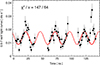 |
Fig. 1. Chandra light curve (black points) in the 0.5–7 keV band of ObsIDs 22648, 22649, and 23182. The bin time is 1500 s. The best-fit sinusoidal is shown in red. The dotted line shows the model’s extrapolation during time intervals with no data. |
In Fig. 2, we show the Lomb-Scargle periodograms (LSPs; Lomb 1976; Scargle 1982) of the C1 dataset. The two LSPs were computed with the version implemented in the Stingray and hendrics Python packages (Huppenkothen et al. 2019b,a; Bachetti 2018; Bachetti et al. 2024); they are based on data from ObsIDs 22648 and 22649 (top panel) and from the whole C1 dataset (bottom panel), and both show a peak at a frequency of ≃3.3 × 10⁻⁵ Hz (≃30 ks). The LSP of the whole C1 dataset shows a broad peak, implying that the modulation is quasi-coherent in nature. Estimating the significance of this peak is tricky. At such low frequencies, one cannot use the standard white noise assumption and compute a frequency-independent threshold (see van der Klis 1989a; Israel & Stella 1996). At the same time, it is difficult to verify the presence of red noise in the LSPs in Fig. 2. When trying to add a power-law component to model it, the parameters are not constrained, likely because the red noise dominates only in the very first bins. Therefore, we lack the necessary statistics to test and quantify the significance of such a component. Finally, we note that we cannot exclude that red noise is the actual origin of the observed possible modulation. However, the presence of a peak in both LSPs would be hard to explain in this case.
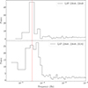 |
Fig. 2. LSPs of the C1 dataset. Top panel: LSP of observations 22648 and 22649. Bottom panel: LSP of the whole C1 dataset. The LSPs have been re-binned with a logarithmic factor of 1.14. The dashed red lines show the frequency of the peak found in the top LSP. At frequencies higher than ν ≃ 0.01 Hz, white noise dominates. Therefore, for visual purposes, we show the LSPs only up to 0.01 Hz. |
Figure 3 shows the 0.5–7 keV, 0.5–2 keV, and 2–7 keV folded light curve of all the Chandra’s C1 observations, phase-folded at the 25.4 ks period derived from the sinusoid fit of C1. In each panel, we also show the value of the semi-amplitude A of the modulation, derived from fitting the data with the function C + Asin[2π(x − x0)/P]. C is the normalised mean flux level and P the period of the modulation, both fixed to 1, while x0 is the phase of the modulation. The amplitude Asoft = (31 ± 6)% is larger in the soft band than in the hard band Ahard = (18 ± 5)%, although we must note that the amplitudes in the two bands are consistent within 3σ. The folded profile, especially in the whole 0.5–7 keV band, appears not strictly sinusoidal. Given the short exposure times compared to the length of the modulation, it is difficult to assess whether the flux goes to background level for a prolonged time, as expected for QPEs, or if the flux keeps oscillating, like in a QPO.
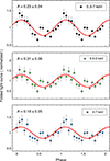 |
Fig. 3. Phase-folded profile of the Chandra C1 light curve. Top panel: Folded light curve in the whole 0.5–7 keV band. Middle panel: Folded light curve in the soft 0.5–2 keV band. Bottom panel: Folded light curve in the hard 2–7 keV band. The input period in the three panels is the same as that of the best-fit sinusoid shown in Fig. 1 (P = 25.4 ± 0.4 ks). A is the semi-amplitude of the modulation. Two cycles are shown in each panel for clarity. |
From a visual inspection of the light curves reported in Appendix A, it is interesting to note that J1257 has shown a similar variability behaviour on other occasions. Throughout 2020, J1257 flux is characterised by a modulating behaviour. For example, during ObsID 22930 (Fig. A.10) one can see two peaks separated by ≃20 ks. During ObsID 0124710101, two flares on top of a steady rise in the flux are also present (Fig. A.1). However, the short duration of the exposures prevents us from performing a detailed analysis of the observed variability.
Finally, we must note that adding the other Chandra observations performed in 2020 (i.e. ObsIDs 22930, 23361, 24853, and 24854) to construct the folded profile progressively diminishes the amplitude of the modulation. The trend continues if we add the older Chandra and XMM-Newton observations. However, this is not surprising and should not be directly considered as an indication of the absence of a real signal. Given the present uncertainty on the period of the possible modulation, we cannot perform a phase connection between observations that were performed months (or even years) before or after the C1 observations. Additionally, if the modulation is quasi-periodic in nature, the period could change significantly among the different epochs, contributing to the loss of amplitude in the folded profile.
3.1.2. Flare-like behaviour
J1257 showed (at least twice) a flaring-like behaviour, in which the count rate suddenly increased by a factor of 5, that is, ObsID 12887 and ObsID 0691610201. The light curve of ObsID 12887 is shown in Fig. A.5. Here, we focus on ObsID 0691610201, which has a higher statistic and allows for a better study of the energy-dependent emission. In the upper panel Fig. 4, we present the XMM-Newton light curve from ObsID 0691610201 in the soft (0.3–1 keV, black points) and hard (1–10 keV, red points) band, together with the hardness ratio (hard/soft) in the lower panel. We tried different energy cuts. Based on the shape of the energy spectrum (see e.g. Fig. 5), we selected a soft band from 0.3 keV to 0.6 keV and a hard band from 1.5 keV to 10 keV or from 2 keV to 10 keV. These choices did not change our results. Therefore, we opted for the cut at 1 keV between the two bands to have a similar number of photons and similar statistics.
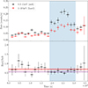 |
Fig. 4. Light curve of J1257 during the XMM-Newton observation 0691610201. Top panel: Light curve in the soft (0.3–1 keV) and hard (1–10 keV) band. Bottom panel: Hardness ratio of the hard count rate over the soft count rate. The red (dashed purple) line shows the result of the fit of the hardness ratio with a constant outside (within) the high-flux phase (highlighted in blue). The corresponding shaded region shows the 1σ confidence interval. The bin time in both panels is 1500 s. |
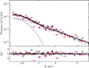 |
Fig. 5. X-ray spectrum (upper panel) and residuals (lower panel) of the J1257, taken with XMM-Newton in June 2000 (ObsID 0124710101). We show data from EPIC/pn (in black), EPIC/MOS1 (in red), and EPIC/MOS2 (in magenta). The best-fitting model is shown with a solid line; the two components, black body and power-law, are shown with the dotted black lines. |
We identified a low-flux state and a high-flux state (highlighted in blue in Fig. 4). After the first ≃18 ks, during which the count rate has a mean value of ≃0.05 counts/s, it rapidly increases of a factor of ∼5 in about 5 ks. After a decrease in the following 5 − 6 ks, this high-flux state ends, but right after it, the count rate seems to rise again. Unfortunately, this rise coincides with the end of the observation. Therefore, we cannot verify whether J1257 is showing the same modulation we detected in the previously shown Chandra observations or a different kind of variability. It is interesting to note, however, that the flare during ObsID 0691610201 has a similar duration (∼10 ks) and peak/out-of-peak flux ratio in the 0.5–7 keV band (∼5) of the flare detected at the end of ObsID 23182, shown in Fig. 1. These similarities could suggest that the two flares are produced by the same mechanism.
To model the evolution of the hardness ratio, we considered the values outside (within) the high-flux state and fitted the hardness ratio with a constant. The result of our fit is shown by the red (purple) solid (dashed) line in Fig. 4. The flux seems to get softer during the high-flux state, but the values of the hardness ratio outside (HRlow = 0.69 ± 0.05) and during (HRhigh = 0.55 ± 0.02) this phase are consistent within 3σ. Therefore, we cannot claim any significant change in the hardness ratio during the observation. We studied the hardness ratio for all the XMM-Newton and Chandra observations reported in Table 1. For the XMM-Newton observations, we used the same 0.3–1/1–10 keV bands, while for Chandra observations we used a soft 0.5–2 keV band and a hard 2–7 keV to meet our requirement of an equal number of photons in the two bands. As for ObsID 0691610201, we always found that a constant is sufficient to model the evolution of the hardness ratio.
3.2. X-ray spectral analysis
The X-ray spectra were analysed with the spectral fitting package XSPEC (Arnaud 1996) version 12.12.1. The spectra were re-binned to have at least 1 count per energy bin, and the modified Cash statistic (W-stat; Cash 1979) was adopted. All X-ray spectra were corrected for foreground interstellar absorption adopting the model TBABS, with NH fixed to the Galactic value 8.4 × 1019 cm−2 (HI4PI Collaboration 2016), using abundances from Wilms et al. (2000), with the photoelectric absorption cross-sections from Verner et al. (1996). All reported uncertainties correspond to 1σ, all reported fluxes and luminosities are corrected for absorption.
J1257 shows significant variability in its spectral behaviour (see Table 2): while a simple power-law model can reproduce satisfactorily the X-ray spectrum of the source in most observations, in some epochs the quality of the fit is significantly improved by the addition of a thermal component and/or a layer of intrinsic absorption (in excess of the Galactic one). We modelled the thermal component with a simple blackbody profile, with temperatures of about kT ∼ 110 eV. This thermal component is mostly detected in observations taken before 2012, as in the latest Chandra observations, the loss of effective area in the soft band (below ≈1 keV; see Plucinsky et al. 2018, 2022) prevents us from constraining its presence. The layer of intrinsic neutral absorption improves the quality of the fit in the most recent observations (from 2012 and in 2020), and it is characterised by a column density in the (0.1 − 2)×1022 cm−2 range. The photon index Γ varies significantly too, spanning a wide range of values, from Γ = 0.8 to Γ = 2.
X-ray spectral parameters of the source in the different epochs.
This spectral evolution is associated with significant long-term variability in the source’s flux. As reported in Fig. 6, the source’s flux varies by a factor of about 3 in timescales of days, both in the soft (0.3–2 keV) and hard (2–10 keV) band. We inspected the correlation between the spectral shape and the flux state of the source and, as highlighted in Fig. 7, J1257 appears to exhibit two distinct behaviours. When the source’s flux is below ≈3 × 10⁻¹³ erg/s/cm2, it shows the full range of spectral steepness described above. When instead the source flux is above the ≈3 × 10⁻¹³ erg/s/cm2 threshold, it seems to exhibit a softer-when-brighter behaviour. However, the heterogeneity of the available dataset (e.g. the limited effective area in the soft X-ray regime of Chandra in the more recent observations, the presence of a poorly constrained local absorber, and the possibility that some spectral changes are linked to the short-term variability) limits a more in-depth analysis of this feature.
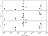 |
Fig. 6. X-ray-unabsorbed flux in the soft 0.3–2 keV band (upper panel), in the hard 2–10 keV band (middle panel), and the photon index (Γ; lower panel) in each epoch. |
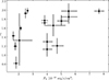 |
Fig. 7. Spectral photon index (Γ) versus X-ray-unabsorbed flux in the 0.3–10 keV band. |
The X-ray spectral properties of the source are listed in Tab. 2. An exemplary spectrum (re-binned for graphical purposes) is shown in Fig. 5, and the rest of the spectra are reported in Appendix B. A visual inspection of the reported spectra highlights the extreme variability in the spectral shape of J1257, corroborating the conclusion that the variations in the photon index of the power-law component, reported in Tab. 2, are intrinsic and not driven by external factors, such as un-modelled absorption components.
4. Discussion
To exclude the possibility that we had detected an extra-nuclear source, we cross-matched J1257 coordinates, as derived by the CIAO source detection tool wavdetect5, with those of the central SMBH as reported in the 2MASS catalogue (Skrutskie et al. 2006). Our analysis confirms that the source showing the possible modulation is the central SMBH. Optical observations of J1257 reveal the presence of a broad Hα emission line (FWHM of ∼2000 − 3000 km s−1) and a Hβ emission line with a FWHM of ∼1000 km s−1, supporting a classification as an intermediate-type Seyfert galaxy (Véron-Cetty & Véron 2010; Toba et al. 2014; Liu et al. 2021; Negus et al. 2024).
Our analysis shows that J1257 possesses peculiar X-ray variability. A repeated modulation, and possibly a flare-like behaviour, is present on the timescales of ≃20 − 30 ks. Unfortunately, although J1257 has been observed multiple times by both Chandra and XMM-Newton, most observations do not last long enough for a definitive classification of this variability. The long-term light curve shows that the source flux can change up to a factor of 3 in a few days, while the spectral analysis reveals that J1257 shows hints of a softer-when-brighter behaviour.
In this section we discuss the most plausible origins of this repeated variability in light of our findings.
4.1. Quasi-periodic modulation candidate
Looking at Fig. 1 and Fig. 2, it is tempting to classify the modulation as a QPO. The modulation seems to be present throughout 2020, as shown by the phase-folded light curve in Fig. 3 and the light curves of ObsIDs 22930, 23361, 24853, and 24854 shown in Appendix A. Although J1257 has been observed multiple times by both Chandra and XMM-Newton, most observations do not last long enough to appreciate a modulation on the timescales of 20–30 ks. Even in the best dataset (C1), we only detect a few cycles of the putative modulation, which is not enough for a firm detection. Therefore, we will limit our discussion to a simple scenario6. Given the uncertainties on the timescale of the modulation, in this section we consider a frequency range of 33 − 50 μHz, which corresponds to the aforementioned 20–30 ks range.
If the variability is indeed caused by a QPO, its centroid frequency can be associated with a fundamental frequency of the accretion disk at the innermost stable circular orbit (ISCO), that is, the minimal radius at which stable circular motion is still possible (see e.g. Jefremov et al. 2015). In this case, the QPO is related to the Keplerian orbital frequency (νϕ), the vertical epicyclic frequency (νθ), or the Lense-Thirring frequency (νLT) of the matter falling onto the SMBH (see e.g. Stella & Vietri 1998; Stella et al. 1999). The three frequencies can be linked to the mass MBH, the radius of the ISCO RISCO, and the dimensionless spin parameter a* of J1257 using the expressions derived by Kato (1990):
![Mathematical equation: $$ \begin{aligned} \nu _\phi =\frac{c^3}{2\pi GM_{\rm BH}}\left[\frac{1}{R_{\rm ISCO}^{3/2}+a_*}\right] \end{aligned} $$](/articles/aa/full_html/2026/02/aa57527-25/aa57527-25-eq26.gif) (1)
(1)
![Mathematical equation: $$ \begin{aligned} \nu _\theta = \nu _\phi \left[1-\frac{4a_*}{R_{\rm ISCO}^{3/2}}+\frac{3a_*^2}{R_{\rm ISCO}^2}\right]^{1/2} \end{aligned} $$](/articles/aa/full_html/2026/02/aa57527-25/aa57527-25-eq27.gif) (2)
(2)
 (3)
(3)
where c is the speed of light and G is the gravitational constant.
As already mentioned in Sect. 1, Liu et al. (2021) derived a mass ∼106.3 M⊙ for J1257, in line with the other SMBHs showing (candidate) QPOs (see e.g. Fig. 5 of Yan et al. 2024). Using this mass estimate and the equations above, testing for −1 ≤ a* ≤ 1, we find that in this scenario the observed frequency range is consistent only with the Lense-Thirring frequency of Eq. (3). However, when compared to other SMBHs showing (candidate) QPOs, it is hard to reconcile the mass of J1257 with the observed timescales of the modulation. By looking again at Fig. 5 of Yan et al. (2024), QPO frequencies of ≃33 − 50 μHz would be extremely low for a SMBH with a mass ∼106.3 M⊙ such as J1257.
4.2. J1257 as a possible QPE candidate
The Chandra light curve in Fig. 1 comprises three main X-ray flares that are close to symmetric, separated by similar time intervals of 51.3 ks and 50.0 ks, and followed by a shorter-duration and higher amplitude burst towards the end of the third observation. The interpretation in terms of a sinusoidal modulation with period of ≃25.4 ks (as derived from our fit in Fig. 1) in which some of the peaks fall within the gaps is not unique. Although the nature of the light curve prevents us from firmly assessing the significance of the putative periodicity, it is worth briefly exploring further possible interpretations. Here, we consider the possibility that the observed variability might be associated with QPEs. This suggestion must be considered as speculative at this stage and would need to be confronted against future, uninterrupted X-ray exposures.
A model in which the sinusoidal modulation is replaced by three Gaussian functions, and the last shorter duration flare is also described with the same function representing QPEs, is shown in the upper panel of Fig. 8. The double QPE structure seen in the third observation is possibly repeated in the first two as well, as hinted by the rapid rise in count rate following the main flares. In fact, adding two Gaussian functions with all parameters fixed to those of the last flare (except centroid) to account for the rise towards the end of the first and second observation returns a statistical result of χ2/d.o.f. = 65/53 as shown in the lower panel of Fig. 8. In this framework, the X-ray light curve could be consistent with the typical QPE one, in which longer and shorter recurrence times (as well as stronger and weaker QPEs) alternate (for one representative example see Miniutti et al. 2023b).
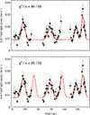 |
Fig. 8. Chandra light curve in the 0.5–7 keV band of ObsIDs 22648, 22649, and 23182, as shown in Fig. 1. The upper and lower panels show in red the best-fitting model 1 and model 2, respectively (see text for details). The model extrapolation within the gaps is shown as a dotted line. |
An interpretation of the X-ray variability in terms of QPEs appears therefore speculative – mostly due to the limited number of observed cycles – but plausible. It is then interesting to consider whether the derived timing parameters (recurrence time and QPE duration) are in line with the overall observed QPE population. To be conservative, we considered the largest possible range in recurrence time between peaks (Trec) and burst duration (Tdur) derived from the single- and double-peak QPE models fitted on the C1 dataset. We infer Trec = 13.1–51.3 ks and Tdur = 9.5-19.5 ks in J1257. These estimates allow us to place J1257 onto the Tdur–Trec plane of the current QPE population (see e.g. Fig. 8 of Arcodia et al. 2025). The location of J1257 in the QPE Tdur–Trec plane is shown in Fig. 9 as a purple area and appears to be consistent with J1257 being part of the QPE family. We note that the Tdur–Trec linear relation (see the best-fitting model in Fig. 9, dashed line) is empirical only and suggests a roughly constant duty cycle for QPEs. The relation has only been studied in the context of EMRI-based QPE models and suggests that QPE emission is dominated by the interaction between the accretion disk and debris that are ablated from an orbiting star at each star-disk collision rather than by the star-disk collision itself (Linial et al. 2025; Mummery 2025). Here, we simply consider it as an indication that the timing properties of the X-ray flares in J1257 are roughly consistent with the overall QPE population.
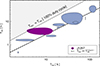 |
Fig. 9. Location of J1257 (purple region) on the Tdur–Trec plane defined by the current QPE population (light blue regions). The grey area represents events with Tdur ≥ Trec that cannot be classified as well-isolated QPEs. We point out that QPEs with long recurrence times and short durations, which would populate the lower-right corner of the plane, are extremely difficult to detect; therefore, the clear correlation seen in the QPE timing plane could be affected, at least partly, by an observational bias. QPE data are taken from Arcodia et al. (2025). The dashed line is a best-fitting relation of the form |

On the other hand, the spectral properties of J1257 are very distinct from those of X-ray QPEs. The latter are thermal-like, soft X-ray flares with typical temperatures of kT ∼ 100 − 200 eV, therefore contributing very marginally above 2 keV. All sources observed thus far exhibit a clear counter-clockwise pattern in the L − T plane during the QPE evolution (see e.g. Fig. 18 in Miniutti et al. 2023b). Conversely, the X-ray flaring activity in J1257 appears to be almost achromatic with only a slightly higher relative amplitude in the soft X-ray band, as shown in Fig. 3.
Besides, and this is the most relevant difference, QPEs are detected above a quiescent X-ray emission that is fully consistent with a post-TDE, compact accretion disk with little to no contribution above ∼2 keV. Instead, the X-ray spectrum of J1257 is clearly that of a standard unobscured type-1 AGN comprising a hard X-ray power law continuum and a soft excess (although the spectral variability of the target is extreme for AGNs; see Fig. 6). The detection of broad optical emission lines confirms the presence of an active nucleus capable of sustaining a mature broad-line region, in contrast with the TDE case. Such differences imply a different accretion flow structure and geometry, which might have an impact on the QPE spectral shape and evolution. No specific model for QPEs in AGNs has been presented thus far, so it is not possible to assess whether the distinct spectral evolution of the flares in J1257 are consistent with QPEs occurring in AGNs (or following a TDE in an AGN), which might be different from that of typical post-TDE QPEs.
We conclude that the X-ray variability pattern in J1257 is reminiscent of QPEs in terms of timing properties but that the flares’ X-ray spectral shape and evolution are not consistent with the current QPE population, preventing us from classifying J1257 as a bona fide QPE source. Theoretical studies of the observational properties of QPE emission in AGNs for the different QPE models proposed so far are needed to make progress, along with uninterrupted X-ray observations that will deliver higher-quality time-resolved spectral data and shed light on the recurrence pattern, if any.
5. Conclusions
We have reported on the timing and spectral analysis of Chandra and XMM-Newton data of J1257, an intermediate-type Seyfert galaxy at z = 0.02. Prompted by the detection of a repeated modulation at timescales of ≃20–30 ks, we found that J1257 has also shown long-term X-ray variability coupled with a complex spectral evolution in the last 20 years, reported here for the first time. Whatever the origin, the results we present in this paper suggest that J1257 is a new specimen of the growing class of SMBHs that show repeated X-ray variability. In particular, it could be either a QPO candidate with a particularly long period or a QPE candidate with an unusually hard spectrum, making J1257 a particularly interesting source. If confirmed, given the possible connection of these phenomena with EMRIs, J1257 could also represent a source of interest for future missions such as LISA with the aim of obtaining a deeper comprehension of the SMBH phenomenology. Due to the limited number of observed cycles, the modulation’s statistical significance cannot be estimated robustly, and both the confirmation of its presence and a detailed characterisation of its spectral-timing properties must await longer, uninterrupted future X-ray observations.
Acknowledgments
We acknowledge the use of the following software: scipy (Virtanen et al. 2020), SAS (Gabriel et al. 2004), CIAO (Fruscione et al. 2006), Stingray (Huppenkothen et al. 2019b,a; Bachetti et al. 2024), hendrics (Bachetti 2018). MI is supported by the AASS Ph.D. joint research programme between the University of Rome “Sapienza” and the University of Rome “Tor Vergata”, with the collaboration of the National Institute of Astrophysics (INAF). GM thanks the Spanish MICIU/AEI/10.13039/501100011033 grants n. PID2020-115325GB-C31 and n. PID2023-147338NB-C21 for support. RA acknowledges financial support from INAF through the grant “INAF-Astronomy Fellowships in Italy 2022 – (GOG)”.
References
- Abramowicz, M. A., Czerny, B., Lasota, J. P., & Szuszkiewicz, E. 1988, ApJ, 332, 646 [Google Scholar]
- Ahn, C. P., Alexandroff, R., Allende Prieto, C., et al. 2012, ApJS, 203, 21 [Google Scholar]
- Amaro-Seoane, P. 2018, Liv. Rev. Relativity, 21, 4 [Google Scholar]
- Amaro-Seoane, P., Gair, J. R., Pound, A., Hughes, S. A., & Sopuerta, C. F. 2015, J. Phys. Conf. Ser., 610, 012002 [Google Scholar]
- Amaro-Seoane, P., Audley, H., Babak, S., et al. 2017, ArXiv e-prints [arXiv:1702.00786] [Google Scholar]
- Arcodia, R., Merloni, A., Nandra, K., et al. 2021, Nature, 592, 704 [NASA ADS] [CrossRef] [Google Scholar]
- Arcodia, R., Liu, Z., Merloni, A., et al. 2024, A&A, 684, A64 [NASA ADS] [CrossRef] [EDP Sciences] [Google Scholar]
- Arcodia, R., Baldini, P., Merloni, A., et al. 2025, ApJ, 989, 13 [Google Scholar]
- Arnaud, K. A. 1996, ASP Conf. Ser., 101, 17 [Google Scholar]
- Bachetti, M. 2018, Astrophysics Source Code Library [record ascl:1805.019] [Google Scholar]
- Bachetti, M., Huppenkothen, D., Stevens, A., et al. 2024, J. Open Source Software, 9, 7389 [Google Scholar]
- Backer, D. C., & Hellings, R. W. 1986, ARA&A, 24, 537 [Google Scholar]
- Bartlett, E. S., Coe, M. J., Israel, G. L., et al. 2017, MNRAS, 466, 4659 [NASA ADS] [Google Scholar]
- Burrows, D. N., Hill, J. E., Nousek, J. A., et al. 2005, Space Sci. Rev., 120, 165 [Google Scholar]
- Casella, P., Ponti, G., Patruno, A., et al. 2008, MNRAS, 387, 1707 [NASA ADS] [CrossRef] [Google Scholar]
- Cash, W. 1979, ApJ, 228, 939 [Google Scholar]
- Chakraborty, J., Kara, E., Masterson, M., et al. 2021, ApJ, 921, L40 [NASA ADS] [CrossRef] [Google Scholar]
- Chakraborty, J., Kara, E., Arcodia, R., et al. 2025, ApJ, 983, L39 [Google Scholar]
- Colpi, M., Danzmann, K., Hewitson, M., et al. 2024, ArXiv e-prints [arXiv:2402.07571] [Google Scholar]
- Esposito, P., Israel, G. L., Sidoli, L., et al. 2013a, MNRAS, 436, 3380 [NASA ADS] [CrossRef] [Google Scholar]
- Esposito, P., Israel, G. L., Sidoli, L., et al. 2013b, MNRAS, 433, 3464 [NASA ADS] [CrossRef] [Google Scholar]
- Esposito, P., Israel, G. L., de Martino, D., et al. 2015, MNRAS, 450, 1705 [Google Scholar]
- Franchini, A., Bonetti, M., Lupi, A., et al. 2023, A&A, 675, A100 [NASA ADS] [CrossRef] [EDP Sciences] [Google Scholar]
- Fruscione, A., McDowell, J. C., Allen, G. E., et al. 2006, SPIE Conf. Ser., 6270, 62701V [Google Scholar]
- Gabriel, C., Denby, M., Fyfe, D. J., et al. 2004, ASP Conf. Ser., 314, 759 [Google Scholar]
- Gaia Collaboration 2020, VizieR On-line Data Catalog: I/350 [Google Scholar]
- Gezari, S. 2021, ARA&A, 59, 21 [NASA ADS] [CrossRef] [Google Scholar]
- Gierliński, M., Middleton, M., Ward, M., & Done, C. 2008, Nature, 455, 369 [CrossRef] [Google Scholar]
- Giustini, M., Miniutti, G., & Saxton, R. D. 2020, A&A, 636, L2 [NASA ADS] [CrossRef] [EDP Sciences] [Google Scholar]
- González-Martín, O., & Vaughan, S. 2012, A&A, 544, A80 [NASA ADS] [CrossRef] [EDP Sciences] [Google Scholar]
- Hernández-García, L., Chakraborty, J., Sánchez-Sáez, P., et al. 2025, Nat. Astron., 9, 895 [Google Scholar]
- HI4PI Collaboration (Ben Bekhti, N., et al.) 2016, A&A, 594, A116 [NASA ADS] [CrossRef] [EDP Sciences] [Google Scholar]
- Huppenkothen, D., Bachetti, M., Stevens, A., et al. 2019a, J. Open Source Software, 4, 1393 [NASA ADS] [CrossRef] [Google Scholar]
- Huppenkothen, D., Bachetti, M., Stevens, A. L., et al. 2019b, ApJ, 881, 39 [Google Scholar]
- Imbrogno, M., Motta, S. E., Amato, R., et al. 2024, A&A, 689, A284 [NASA ADS] [CrossRef] [EDP Sciences] [Google Scholar]
- Ingram, A. R., & Motta, S. E. 2019, New Astron. Rev., 85, 101524 [Google Scholar]
- Ingram, A., Done, C., & Fragile, P. C. 2009, MNRAS, 397, L101 [Google Scholar]
- Israel, G. L., & Stella, L. 1996, ApJ, 468, 369 [Google Scholar]
- Israel, G. L., Esposito, P., Rodríguez Castillo, G. A., & Sidoli, L. 2016, MNRAS, 462, 4371 [Google Scholar]
- Jansen, F., Lumb, D., Altieri, B., et al. 2001, A&A, 365, L1 [NASA ADS] [CrossRef] [EDP Sciences] [Google Scholar]
- Jefremov, P. I., Tsupko, O. Y., & Bisnovatyi-Kogan, G. S. 2015, Phys. Rev. D, 91, 124030 [NASA ADS] [CrossRef] [Google Scholar]
- Kato, S. 1990, PASJ, 42, 99 [NASA ADS] [Google Scholar]
- Kejriwal, S., Witzany, V., Zajaček, M., Pasham, D. R., & Chua, A. J. K. 2024, MNRAS, 532, 2143 [Google Scholar]
- Komossa, S. 2015, J. High Energy Astrophys., 7, 148 [Google Scholar]
- Lin, D., Irwin, J. A., Godet, O., Webb, N. A., & Barret, D. 2013, ApJ, 776, L10 [NASA ADS] [CrossRef] [Google Scholar]
- Linial, I., & Metzger, B. D. 2023, ApJ, 957, 34 [NASA ADS] [CrossRef] [Google Scholar]
- Linial, I., Metzger, B. D., & Quataert, E. 2025, ApJ, 991, 147 [Google Scholar]
- Liu, W.-J., Lira, P., Yao, S., et al. 2021, ApJ, 915, 63 [NASA ADS] [CrossRef] [Google Scholar]
- Lomb, N. R. 1976, Ap&SS, 39, 447 [Google Scholar]
- Lui, L., Torres-Orjuela, A., Chowdhury, R. K., & Dai, L. 2025, ArXiv e-prints [arXiv:2508.07961] [Google Scholar]
- Lyu, M., Méndez, M., Zhang, G., & Keek, L. 2015, MNRAS, 454, 541 [NASA ADS] [CrossRef] [Google Scholar]
- Masterson, M., Kara, E., Ricci, C., et al. 2022, ApJ, 934, 35 [NASA ADS] [CrossRef] [Google Scholar]
- Masterson, M., Kara, E., Panagiotou, C., et al. 2025, Nature, 638, 370 [Google Scholar]
- Miniutti, G., Saxton, R. D., Giustini, M., et al. 2019, Nature, 573, 381 [Google Scholar]
- Miniutti, G., Giustini, M., Arcodia, R., et al. 2023a, A&A, 674, L1 [NASA ADS] [CrossRef] [EDP Sciences] [Google Scholar]
- Miniutti, G., Giustini, M., Arcodia, R., et al. 2023b, A&A, 670, A93 [NASA ADS] [CrossRef] [EDP Sciences] [Google Scholar]
- Morgan, E. H., Remillard, R. A., & Greiner, J. 1997, ApJ, 482, 993 [NASA ADS] [CrossRef] [Google Scholar]
- Motch, C., Ricketts, M. J., Page, C. G., Ilovaisky, S. A., & Chevalier, C. 1983, A&A, 119, 171 [Google Scholar]
- Motta, S. E., Franchini, A., Lodato, G., & Mastroserio, G. 2018, MNRAS, 473, 431 [NASA ADS] [CrossRef] [Google Scholar]
- Mummery, A. 2025, ArXiv e-prints [arXiv:2504.21456] [Google Scholar]
- Negus, J., Comerford, J. M., & Sánchez, F. M. 2024, ApJ, 971, 92 [Google Scholar]
- Nicholl, M., Pasham, D. R., Mummery, A., et al. 2024, Nature, 634, 804 [CrossRef] [Google Scholar]
- Pasham, D. R., Tombesi, F., Suková, P., et al. 2024, Sci. Adv., 10, eadj8898 [Google Scholar]
- Plucinsky, P. P., Bogdan, A., Marshall, H. L., & Tice, N. W. 2018, SPIE Conf. Ser., 10699, 106996B [NASA ADS] [Google Scholar]
- Plucinsky, P. P., Bogdan, A., & Marshall, H. L. 2022, SPIE Conf. Ser., 12181, 121816X [Google Scholar]
- Quintin, E., Webb, N. A., Guillot, S., et al. 2023, A&A, 675, A152 [NASA ADS] [CrossRef] [EDP Sciences] [Google Scholar]
- Rees, M. J. 1988, Nature, 333, 523 [Google Scholar]
- Remillard, R. A., & McClintock, J. E. 2006, ARA&A, 44, 49 [Google Scholar]
- Ricci, C., Loewenstein, M., Kara, E., et al. 2021, ApJS, 255, 7 [NASA ADS] [CrossRef] [Google Scholar]
- Scargle, J. D. 1982, ApJ, 263, 835 [Google Scholar]
- Shu, X. W., Wang, S. S., Dou, L. M., et al. 2018, ApJ, 857, L16 [NASA ADS] [CrossRef] [Google Scholar]
- Sidoli, L., Esposito, P., Motta, S. E., Israel, G. L., & Rodríguez Castillo, G. A. 2016, MNRAS, 460, 3637 [NASA ADS] [CrossRef] [Google Scholar]
- Sidoli, L., Israel, G. L., Esposito, P., Rodríguez Castillo, G. A., & Postnov, K. 2017, MNRAS, 469, 3056 [CrossRef] [Google Scholar]
- Skrutskie, M. F., Cutri, R. M., Stiening, R., et al. 2006, AJ, 131, 1163 [NASA ADS] [CrossRef] [Google Scholar]
- Smith, K. L., Mushotzky, R. F., Boyd, P. T., & Wagoner, R. V. 2018, ApJ, 860, L10 [NASA ADS] [CrossRef] [Google Scholar]
- Smith, K. L., Tandon, C. R., & Wagoner, R. V. 2021, ApJ, 906, 92 [NASA ADS] [CrossRef] [Google Scholar]
- Stella, L., & Vietri, M. 1998, ApJ, 492, L59 [NASA ADS] [CrossRef] [Google Scholar]
- Stella, L., Vietri, M., & Morsink, S. M. 1999, ApJ, 524, L63 [CrossRef] [Google Scholar]
- Strüder, L., Briel, U., Dennerl, K., et al. 2001, A&A, 365, L18 [Google Scholar]
- Tagger, M., & Pellat, R. 1999, A&A, 349, 1003 [NASA ADS] [Google Scholar]
- Toba, Y., Oyabu, S., Matsuhara, H., et al. 2014, ApJ, 788, 45 [Google Scholar]
- Turner, M. J. L., Abbey, A., Arnaud, M., et al. 2001, A&A, 365, L27 [CrossRef] [EDP Sciences] [Google Scholar]
- van der Klis, M. 1989a, NATO Advanced Study Institute (ASI) Ser. C, 262, 27 [Google Scholar]
- van der Klis, M. 1989b, ARA&A, 27, 517 [NASA ADS] [CrossRef] [Google Scholar]
- Verner, D. A., Ferland, G. J., Korista, K. T., & Yakovlev, D. G. 1996, ApJ, 465, 487 [Google Scholar]
- Véron-Cetty, M. P., & Véron, P. 2010, A&A, 518, A10 [Google Scholar]
- Vikhlinin, A., Churazov, E., Gilfanov, M., et al. 1994, ApJ, 424, 395 [NASA ADS] [CrossRef] [Google Scholar]
- Virtanen, P., Gommers, R., Oliphant, T. E., et al. 2020, NatMe, 17, 261 [NASA ADS] [Google Scholar]
- Weisskopf, M. C., Tananbaum, H. D., Van Speybroeck, L. P., & O’Dell, S. L. 2000, SPIE Conf. Ser., 4012, 2 [Google Scholar]
- Wevers, T., French, K. D., Zabludoff, A. I., et al. 2024, ApJ, 970, L23 [NASA ADS] [CrossRef] [Google Scholar]
- Wilms, J., Allen, A., & McCray, R. 2000, ApJ, 542, 914 [Google Scholar]
- Xia, R., Liu, H., & Xue, Y. 2024, ApJ, 961, L32 [Google Scholar]
- Xia, R., Liu, H., & Xue, Y. 2025, ArXiv e-prints [arXiv:2503.05158] [Google Scholar]
- Xiao, T., Barth, A. J., Greene, J. E., et al. 2011, ApJ, 739, 28 [NASA ADS] [CrossRef] [Google Scholar]
- Yan, Y. K., Zhang, P., Liu, Q. Z., et al. 2024, A&A, 691, A7 [NASA ADS] [CrossRef] [EDP Sciences] [Google Scholar]
- Zhang, H., Yang, S., & Dai, B. 2023, ApJ, 946, 52 [Google Scholar]
- Zhong, X.-G., Wang, J.-C., Chen, Y.-Y., & Yu, X.-L. 2024, Res. Astron. Astrophys., 24, 065015 [Google Scholar]
- Zhou, X.-L., Yuan, W., Pan, H.-W., & Liu, Z. 2015, ApJ, 798, L5 [Google Scholar]
A note of warning is needed. Tempting as it is, one should use these relations with care and always verify the results with independent estimates, since (sub-)millihertz QPOs are also detected in X-ray binaries that host both stellar-mass (MBH ≲ 10 − 20 M⊙) black holes (see e.g. Vikhlinin et al. 1994; Morgan et al. 1997) and neutron stars (see e.g. Lyu et al. 2015; Sidoli et al. 2016; Imbrogno et al. 2024).
For a list of possible, more complicated models explaining QPOs in AGNs, see e.g. Table 1 of Pasham et al. (2024).
Appendix A: Light curves
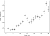 |
Fig. A.1. XMM-Newton light curve in the 0.3–10 keV band during ObsID 0124710101. |
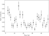 |
Fig. A.2. XMM-Newton light curve in the 0.3–10 keV band during ObsID 0403150201. |
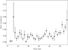 |
Fig. A.3. XMM-Newton light curve in the 0.3–10 keV band during ObsID 0403150101. |
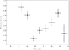 |
Fig. A.4. XMM-Newton light curve in the 0.3–10 keV band during ObsID 0652310401. |
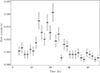 |
Fig. A.5. Chandra light curve in the 0.5–7 keV band duèring ObsID 12887. |
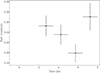 |
Fig. A.6. XMM-Newton light curve in the 0.3–10 keV band during ObsID 0652310801. |
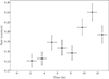 |
Fig. A.7. XMM-Newton light curve in the 0.3–10 keV band during ObsID 0652310901. |
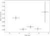 |
Fig. A.8. XMM-Newton light curve in the 0.3–10 keV band during ObsID 0652311001. |
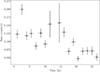 |
Fig. A.9. XMM-Newton light curve in the 0.3–10 keV band during ObsID 0691610301. |
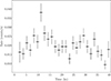 |
Fig. A.10. Chandra light curve in the 0.5–7 keV band during ObsID 22930. |
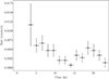 |
Fig. A.11. Chandra light curve in the 0.5–7 keV band during ObsID 23361. |
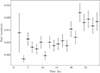 |
Fig. A.12. Chandra light curve in the 0.5–7 keV band during ObsID 24853. |
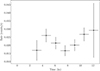 |
Fig. A.13. Chandra light curve in the 0.5–7 keV band during ObsID 24854. |
Appendix B: Spectra
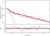 |
Fig. B.1. XMM-Newton spectrum during ObsID 0403150201. |
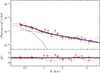 |
Fig. B.2. XMM-Newton spectrum during ObsID 0403150101. |
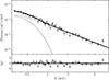 |
Fig. B.3. XMM-Newton spectrum during ObsID 0652310401. |
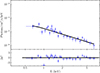 |
Fig. B.4. Chandra spectrum during ObsID 12887. |
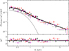 |
Fig. B.5. XMM-Newton spectrum during ObsID 0652310801. |
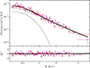 |
Fig. B.6. XMM-Newton spectrum during ObsID 0652310901. |
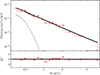 |
Fig. B.7. XMM-Newton spectrum during ObsID 0652311001. |
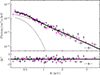 |
Fig. B.8. XMM-Newton spectrum during ObsID 0691610201. |
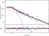 |
Fig. B.9. XMM-Newton spectrum during ObsID 0691610301. |
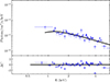 |
Fig. B.10. Chandra spectrum during ObsID 22648. |
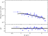 |
Fig. B.11. Chandra spectrum during ObsID 22649. |
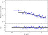 |
Fig. B.12. Chandra spectrum during ObsID 23182. |
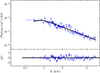 |
Fig. B.13. Chandra spectrum during ObsID 22930. |
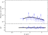 |
Fig. B.14. Chandra spectrum during ObsID 23361. |
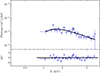 |
Fig. B.15. Chandra spectrum during ObsID 24853. |
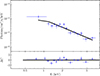 |
Fig. B.16. Chandra spectrum during ObsID 24854. |
All Tables
All Figures
|
Fig. 1. Chandra light curve (black points) in the 0.5–7 keV band of ObsIDs 22648, 22649, and 23182. The bin time is 1500 s. The best-fit sinusoidal is shown in red. The dotted line shows the model’s extrapolation during time intervals with no data. |
| In the text | |
|
Fig. 2. LSPs of the C1 dataset. Top panel: LSP of observations 22648 and 22649. Bottom panel: LSP of the whole C1 dataset. The LSPs have been re-binned with a logarithmic factor of 1.14. The dashed red lines show the frequency of the peak found in the top LSP. At frequencies higher than ν ≃ 0.01 Hz, white noise dominates. Therefore, for visual purposes, we show the LSPs only up to 0.01 Hz. |
| In the text | |
|
Fig. 3. Phase-folded profile of the Chandra C1 light curve. Top panel: Folded light curve in the whole 0.5–7 keV band. Middle panel: Folded light curve in the soft 0.5–2 keV band. Bottom panel: Folded light curve in the hard 2–7 keV band. The input period in the three panels is the same as that of the best-fit sinusoid shown in Fig. 1 (P = 25.4 ± 0.4 ks). A is the semi-amplitude of the modulation. Two cycles are shown in each panel for clarity. |
| In the text | |
|
Fig. 4. Light curve of J1257 during the XMM-Newton observation 0691610201. Top panel: Light curve in the soft (0.3–1 keV) and hard (1–10 keV) band. Bottom panel: Hardness ratio of the hard count rate over the soft count rate. The red (dashed purple) line shows the result of the fit of the hardness ratio with a constant outside (within) the high-flux phase (highlighted in blue). The corresponding shaded region shows the 1σ confidence interval. The bin time in both panels is 1500 s. |
| In the text | |
|
Fig. 5. X-ray spectrum (upper panel) and residuals (lower panel) of the J1257, taken with XMM-Newton in June 2000 (ObsID 0124710101). We show data from EPIC/pn (in black), EPIC/MOS1 (in red), and EPIC/MOS2 (in magenta). The best-fitting model is shown with a solid line; the two components, black body and power-law, are shown with the dotted black lines. |
| In the text | |
|
Fig. 6. X-ray-unabsorbed flux in the soft 0.3–2 keV band (upper panel), in the hard 2–10 keV band (middle panel), and the photon index (Γ; lower panel) in each epoch. |
| In the text | |
|
Fig. 7. Spectral photon index (Γ) versus X-ray-unabsorbed flux in the 0.3–10 keV band. |
| In the text | |
|
Fig. 8. Chandra light curve in the 0.5–7 keV band of ObsIDs 22648, 22649, and 23182, as shown in Fig. 1. The upper and lower panels show in red the best-fitting model 1 and model 2, respectively (see text for details). The model extrapolation within the gaps is shown as a dotted line. |
| In the text | |
|
Fig. 9. Location of J1257 (purple region) on the Tdur–Trec plane defined by the current QPE population (light blue regions). The grey area represents events with Tdur ≥ Trec that cannot be classified as well-isolated QPEs. We point out that QPEs with long recurrence times and short durations, which would populate the lower-right corner of the plane, are extremely difficult to detect; therefore, the clear correlation seen in the QPE timing plane could be affected, at least partly, by an observational bias. QPE data are taken from Arcodia et al. (2025). The dashed line is a best-fitting relation of the form |
| In the text | |
|
Fig. A.1. XMM-Newton light curve in the 0.3–10 keV band during ObsID 0124710101. |
| In the text | |
|
Fig. A.2. XMM-Newton light curve in the 0.3–10 keV band during ObsID 0403150201. |
| In the text | |
|
Fig. A.3. XMM-Newton light curve in the 0.3–10 keV band during ObsID 0403150101. |
| In the text | |
|
Fig. A.4. XMM-Newton light curve in the 0.3–10 keV band during ObsID 0652310401. |
| In the text | |
|
Fig. A.5. Chandra light curve in the 0.5–7 keV band duèring ObsID 12887. |
| In the text | |
|
Fig. A.6. XMM-Newton light curve in the 0.3–10 keV band during ObsID 0652310801. |
| In the text | |
|
Fig. A.7. XMM-Newton light curve in the 0.3–10 keV band during ObsID 0652310901. |
| In the text | |
|
Fig. A.8. XMM-Newton light curve in the 0.3–10 keV band during ObsID 0652311001. |
| In the text | |
|
Fig. A.9. XMM-Newton light curve in the 0.3–10 keV band during ObsID 0691610301. |
| In the text | |
|
Fig. A.10. Chandra light curve in the 0.5–7 keV band during ObsID 22930. |
| In the text | |
|
Fig. A.11. Chandra light curve in the 0.5–7 keV band during ObsID 23361. |
| In the text | |
|
Fig. A.12. Chandra light curve in the 0.5–7 keV band during ObsID 24853. |
| In the text | |
|
Fig. A.13. Chandra light curve in the 0.5–7 keV band during ObsID 24854. |
| In the text | |
|
Fig. B.1. XMM-Newton spectrum during ObsID 0403150201. |
| In the text | |
|
Fig. B.2. XMM-Newton spectrum during ObsID 0403150101. |
| In the text | |
|
Fig. B.3. XMM-Newton spectrum during ObsID 0652310401. |
| In the text | |
|
Fig. B.4. Chandra spectrum during ObsID 12887. |
| In the text | |
|
Fig. B.5. XMM-Newton spectrum during ObsID 0652310801. |
| In the text | |
|
Fig. B.6. XMM-Newton spectrum during ObsID 0652310901. |
| In the text | |
|
Fig. B.7. XMM-Newton spectrum during ObsID 0652311001. |
| In the text | |
|
Fig. B.8. XMM-Newton spectrum during ObsID 0691610201. |
| In the text | |
|
Fig. B.9. XMM-Newton spectrum during ObsID 0691610301. |
| In the text | |
|
Fig. B.10. Chandra spectrum during ObsID 22648. |
| In the text | |
|
Fig. B.11. Chandra spectrum during ObsID 22649. |
| In the text | |
|
Fig. B.12. Chandra spectrum during ObsID 23182. |
| In the text | |
|
Fig. B.13. Chandra spectrum during ObsID 22930. |
| In the text | |
|
Fig. B.14. Chandra spectrum during ObsID 23361. |
| In the text | |
|
Fig. B.15. Chandra spectrum during ObsID 24853. |
| In the text | |
|
Fig. B.16. Chandra spectrum during ObsID 24854. |
| In the text | |
Current usage metrics show cumulative count of Article Views (full-text article views including HTML views, PDF and ePub downloads, according to the available data) and Abstracts Views on Vision4Press platform.
Data correspond to usage on the plateform after 2015. The current usage metrics is available 48-96 hours after online publication and is updated daily on week days.
Initial download of the metrics may take a while.