| Issue |
A&A
Volume 706, February 2026
|
|
|---|---|---|
| Article Number | A62 | |
| Number of page(s) | 20 | |
| Section | Galactic structure, stellar clusters and populations | |
| DOI | https://doi.org/10.1051/0004-6361/202557529 | |
| Published online | 02 February 2026 | |
Stellar masses and mass ratios for Gaia open cluster members
1
Departament de Física Quàntica i Astrofísica (FQA), Universitat de Barcelona (UB),
C Martí i Franquès, 1,
08028
Barcelona,
Spain
2
Institut de Ciències del Cosmos (ICCUB), Universitat de Barcelona (UB),
C Martí i Franquès, 1,
08028
Barcelona,
Spain
3
Institut d’Estudis Espacials de Catalunya (IEEC),
Edifici RDIT, Campus UPC,
08860
Castelldefels (Barcelona),
Spain
4
Astrophysics Division, Shanghai Astronomical Observatory, Chinese Academy of Sciences,
80 Nandan Road,
Shanghai
200030,
China
5
School of Astronomy and Space Science, University of Chinese Academy of Sciences,
No. 19A, Yuquan Road,
Beijing
100049,
China
6
Universidade da Coruña (UDC), Department of Computer Science and Information Technologies,
Campus de Elviña s/n,
15071,
A Coruña,
Galiza,
Spain
★ Corresponding author: This email address is being protected from spambots. You need JavaScript enabled to view it.
Received:
2
October
2025
Accepted:
5
December
2025
Abstract
Context. Unresolved binaries in star clusters can bias stellar and cluster mass estimates. A proper treatment is therefore essential for studying the cluster dynamics and evolution.
Aims. We develop a fast and robust framework for jointly deriving stellar masses and multiplicity statistics of member stars, together with optimal cluster parameters.
Methods. We used Gaia DR3 parallaxes together with multi-band photometry of open cluster (OC) members to infer stellar masses and binary mass ratios through simulation-based inference (SBI), while iteratively fitting the cluster parameters. The validation of our SBI framework on simulated clusters demonstrates that the inclusion of infrared photometry significantly improves the detection of low mass-ratio binaries. The minimum mass-ratio threshold for reliably identifying unresolved binaries depends on the cluster properties and the available photometry, but typically lies below q = 0.5.
Results. Applying our method to 42 well-populated OCs, we derived a catalogue of stellar masses and mass ratios for 27 201 stars achieving typical uncertainties of 0.08 in q and 0.01 M⊙ in the primary stellar mass. We analysed the archetype OCs M67 and NGC 2360 in detail, including mass segregation and mass-ratio distribution, and derived multiplicity fractions for the rest of the sample. We find evidence that the high mass ratio (q ≥ 0.6) binary fraction is strongly correlated with the age and weakly anti-correlated with the cluster metallicity. Furthermore, the variation in the binary fraction with stellar mass in OCs strongly agrees with the observed dependence for field stars with masses higher than ≳0.6 M⊙.
Conclusions. Our work paves a path for future population-level investigations of multiplicity statistics and precision stellar masses in extended OC samples.
Key words: methods: data analysis / methods: statistical / binaries: general / open clusters and associations: general / solar neighborhood
© The Authors 2026
 Open Access article, published by EDP Sciences, under the terms of the Creative Commons Attribution License (https://creativecommons.org/licenses/by/4.0), which permits unrestricted use, distribution, and reproduction in any medium, provided the original work is properly cited.
This article is published in open access under the Subscribe to Open model. This email address is being protected from spambots. You need JavaScript enabled to view it. to support open access publication.
1 Introduction
Star clusters serve as natural laboratories for studying stellar evolution and dynamics because they consist of coeval stellar populations with very similar chemical properties (e.g. Janes & Adler 1982; Kalirai & Richer 2010; Kamdar et al. 2019; Castro-Ginard et al. 2021). They are also considered the progenitors of most stars in the Milky Way (MW) disc (Lada & Lada 2003; Krumholz et al. 2019). On the other hand, multiplicity is widely recognised as a ubiquitous feature among the Galactic field stellar population (Offner et al. 2023), with about 50% solar-type stars observed as part of multiple systems (e.g. Fuhrmann et al. 2017; Moe & Di Stefano 2017). The study of multiplicity in open clusters (OCs) can therefore provide valuable insights into the origin and evolution of binary star systems (e.g. Ebrahimi et al. 2022; Cordoni et al. 2023). Moreover, diverse stellar environments in clusters can help us understand how binary system statistics such as the multiplicity fraction and the mass ratio (q) distribution evolve (Cournoyer-Cloutier et al. 2021; Guszejnov et al. 2023; Pavlík et al. 2025), in addition to providing crucial insights about linking the formation mechanisms of these systems with their observed present-day properties in the Galactic field (Goodwin & Kroupa 2005; Parker et al. 2009).
Historically, unresolved binaries have been linked to increased scatter along the main sequence (MS) in colourmagnitude diagrams (CMDs; Schlesinger 1975). van de Kamp (1968) and Bettis (1977) were among the first to discuss their prevalence in OCs. Classical studies such as those of Duquennoy & Mayor (1991); Raghavan et al. (2010); Moe & Di Stefano (2017) provided baseline statistics for binary fractions in the field. In parallel, efforts using photometric methods in globular clusters (Ivanova et al. 2005; Milone et al. 2012) and N-body simulations (Heggie 1975; Portegies Zwart et al. 2001; Hurley et al. 2007; Kaczmarek et al. 2011) showed that binary fractions evolve dynamically over time due to mass segregation, tidal stripping, and stellar exchange encounters. These effects can alter the binary population along with the present-day mass function, making simple corrections for unresolved systems often insufficient when estimating OC mass distributions and total masses (Rastello et al. 2020).
With its unprecedented precision, the Gaia mission (Gaia Collaboration 2016) has revolutionised our ability to detect multiplicity signatures through photometry, astrometry, and spectroscopy (Gaia Collaboration 2018, 2023a; Belokurov et al. 2020; Castro-Ginard et al. 2024; Li et al. 2025). This opens new avenues for studying unresolved binaries in OCs across the Milky Way, where detection methods previously relied on timeconsuming spectroscopic (Torres 2020; Torres et al. 2021) or eclipsing binary surveys (Mermilliod et al. 1992; Mazur et al. 1995; Brewer et al. 2016; Brogaard et al. 2021).
The effect of binaries on the dynamics of OCs has intensively been studied using N-body simulations in the past 50 years (Heggie 1975; Hurley et al. 2005; Marks et al. 2011; Geller et al. 2013, 2015). For example, Parker et al. (2009) predicted that wide binaries are destroyed after a few crossing times. This prediction was later corroborated with Hubble data for globular clusters (Milone et al. 2012) and with Gaia DR2 data for OCs (Deacon & Kraus 2020). The advent of Gaia has already allowed several in-depth studies of binaries in individual OCs to be conducted using multi-band photometry (e.g. Cohen et al. 2020; Li et al. 2020; Malofeeva et al. 2022, 2023; Childs et al. 2024). Larger samples (∼200) of OCs with binary statistics are also starting to be assembled (e.g. Donada et al. 2023; Jiang et al. 2024). Mostly, however, the modelling does not allow for precise determinations of individual mass-ratios. In this paper, we attempt to obtain precise individual stellar masses and mass-ratios of unresolved binaries in OCs using a self-consistent (although still unavoidably model-dependent) way.
Our paper is structured as follows: in Sect. 2 we summarise the data along with the selection of the OC sample used in this study. Section 3 describes the method we employed to simultaneously infer individual stellar masses, mass ratios of unresolved binaries, and cluster parameters such as age, distance, and interstellar extinction. In Sect. 4, we test our method on simulated star clusters and proceed to present the results for the selected Gaia DR3 OCs in Sect. 5 (the science results are presented in Sect. 5). We provide a comparison with the literature in Sect. 6 and discuss the results in a broader context in Sect. 7. Our conclusions are presented in Sect. 8.
2 Data
We made use of multi-band photometry1 from the Two Micron All Sky Survey (2MASS; Skrutskie et al. 2006), the Wide-field Infrared Survey Explorer (WISE; Wright et al. 2010), and Gaia along with Gaia DR3 parallax measurements of stars in OCs. To maximise homogeneity, we used the OC membership lists provided by Hunt & Reffert (2024, hereafter HR24) for 7167 cluster or moving group candidates, 3530 of which were classified as reliable clusters2 by the authors. We also included two objects, UPK 303 and UPK 612 (classified as moving groups by HR24), due to their very well-defined CMDs. Further, only OCs3 within 2 kpc from the Sun were considered in order to limit the impact of parallax uncertainties and interstellar extinction.
Although several previous studies have estimated the ages, distances, and line-of-sight extinctions of clusters (e.g. Bossini et al. 2019; Cantat-Gaudin et al. 2020; Dias et al. 2021; Hunt & Reffert 2023; Cavallo et al. 2024), we found that many of these solutions do not optimally reproduce the observed CMDs, which renders them unsuitable for a robust characterisation of unresolved binaries. Hence, we re-estimated the cluster parameters (see Sect. 3.5) while using spectroscopically derived metallic-ities compiled by Joshi et al. (2024). In addition, we selected OCs with well-defined densely populated main sequences and no evidence of differential extinction in their CMDs. This yielded 144 candidates. We classified these OCs into three categories, poor, good, and very good, based on the reliability of the cluster parameters inferred by our method. Of the 144 candidates, 42 (∼32%) fall into the very good category and are the focus of this study (see Sect. 5).
3 Method
Our pipeline consisted of the following: (i) we employed simulation-based inference (SBI, e.g. Greenberg et al. 2019; Papamakarios et al. 2021; Cranmer et al. 2020) to infer the stellar parameters (Sects. 3.1 and 3.2), (ii) we estimated the cluster parameters through an iterative procedure (Sects. 3.3 and 3.5), and (iii) we used the observed mass dependence of the binary fraction (Sect. 3.4) to refine the joint mass-q posterior. We show a schematic diagram for our method in Fig. 1.
3.1 Simulation-based inference of stellar parameters
We inferred the posterior distribution of astrophysical parameters for each star from its observed multi-band photometry provided by Gaia, 2MASS, and WISE, in addition to the Gaia parallax (ϖ). The parameters included the primary mass (MA), metallicity ([Fe/H])4, age (log10(Age [yr])), mass ratio (q), distance modulus (μ), and line-of-sight extinction at 550 nm (AV). We adopted a similar method as proposed by Wallace (2024) and employed SBI, which avoids the need for an explicit likelihood function. In particular, we applied a neural posterior estimation (NPE; e.g. Papamakarios & Murray 2016), in which a neural network was trained on simulated data to parametrise a density estimator that approximates the posterior distribution. This approach is significantly faster than traditional inference methods and can be efficiently scaled over a large sample, making it particularly useful for homogeneous studies of OC members.
3.2 Simulated training dataset
In order to test the effect of systematic uncertainties in stellar evolutionary models, we tested two sets of stellar models, namely the PARSEC (Bressan et al. 2012) and the MIST (Dotter 2016; Choi et al. 2016) libraries. Owing to notable differences in the predicted photometry of low-mass stars between the two sets of isochrones (e.g. Choi et al. 2016), however, we adopted the PARSEC isochrones to facilitate a direct comparison with previous studies, although our approach is readily applicable to any theoretical stellar model. We simulated the corresponding observables of about two million stars that broadly resemble a typical Galactic cluster population, with the prior distributions taken from Table 1. We adopted these broad priors to include almost all physically plausible combinations of the respective parameters so that our method can be applied to novel data without introducing significant systematic biases. The apparent magnitudes were obtained by assigning a distance, d (pc), and a line-of-sight extinction, AV (mag), and we used the extinction coefficients5 for the Gaia, 2MASS (following Danielski et al. 2018), and WISE passbands (Yuan et al. 2013). The true parallax, w, was computed as the inverse of the simulated distances. While simulating the training dataset, we occasionally generated unphysical stars (e.g. stars that were too massive for the simulated age) or very faint stars (i.e. G ≳ 21 mag), which are mostly not detected by Gaia. These stars were therefore subsequently removed from the training data. Moreover, as shown in Table 1, we used a lower limit of 0.1 M⊙ on the stellar mass for our simulations. When the stellar mass of the companion was lower than this threshold, the system was therefore treated as a single star. This resulted in an excess of simulated systems with a mass ratio q = 0. Figure E.5 shows the resulting distribution of the astrophysical parameters of the simulated unresolved binaries and single stars.
Since SBI requires the training data to closely resemble the real data (Kelly et al. 2025), we incorporated observational uncertainties by directly injecting noise into the simulated observables instead of treating the uncertainties as separate variables during training. This approach helped us to avoid assuming that the mean values of the simulated observables are representative of the true ones. We used a method similar to that described by Wallace (2024) to simulate the uncertainties in the photometric magnitudes and parallaxes by interpolating their observed dependence on the apparent magnitudes in the real data (e.g. Fabricius et al. 2021).
We note that the colour deviation between the observed Gaia CMDs of OCs and the theoretical isochrones (e.g. Wang et al. 2025) has been studied frequently, especially in the low-mass regime (M ~ 0.3-0.6M⊙). This might affect our results for a few OCs in the mass range we are interested in, and we discuss this in Sects. 5 and 7.
These simulations were then used to train the neural network and obtain the posterior distributions using SBI6 provided the photometric and parallax measurements of the HR24 cluster members. Multi-band photometry from the three surveys is not available for each cluster member, however, and we therefore derived three posteriors, each corresponding to different subsets based on the availability of photometric measurements (see Fig. A.1). After multiple attempts, we found that 20 000 posterior samples7 for each star worked best in the current scenario.
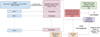 |
Fig. 1 Schematic diagram showing the workflow with which we obtained the joint-posterior distribution of the stellar mass and mass ratio while iteratively updating the cluster parameters until convergence. |
Prior distributions for the model parameters we used to generate the simulated training dataset.
3.3 Applying cluster parameter priors
As shown in Fig. 1, we incorporated the cluster parameter information by assigning weights to SBI posterior samples of cluster members while assuming a Gaussian distribution in log(Age), distance, [Fe/H], and AV. These Gaussian distributions were truncated at ±5σ, which led to some photometric outliers whose posteriors were inconsistent with the assumed cluster parameters. In this entire procedure, the resulting weight assigned to each posterior sample was approximated by a multiplication of the individual weights corresponding to each Gaussian prior. Although this is not ideal because the derived cluster parameters are expected to be correlated, and the correct procedure would involve sampling from the conditional posterior while keeping the cluster parameters fixed, we do not adopt this approach for the following reasons: (a) we wished to simultaneously infer the log(Age), distance, and AV without any prior information, (b) the availability of the computational resources required for the traditional Markov chain Monte Carlo (MCMC) method used in such a sampling is limited, and (c) as shown in Appendix C, our method of assigning weights to posterior samples does not significantly affect the results.
Figure 2 illustrates the use of prior information about the cluster parameters in the inference of masses and mass ratios of the cluster members. The resulting modes of the weighted posterior distributions recover the underlying simulated masses and mass ratios with high precision, in contrast to the case where the cluster parameter information is not incorporated. For the weighted posteriors, only 175 out of the 20 000 samples had a non-zero weight. This is slightly below the typical valid sample rate of about 4%.
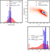 |
Fig. 2 Corner plots of SBI posteriors for a simulated low-mass binary star (MA ~ 0.76 M⊙, q ~ 0.85, d = 1 kpc, AV ~ 0.48 mag, log(Age) [dex] = 9.5, and [Fe/H] [dex] = 0.0) with typical Gaia DR3 and 2MASS/WISE uncertainties for two cases: without (red) and with (blue) prior information about the cluster parameters to obtain the weighted posterior distribution. |
3.4 Mass-ratio prior
After applying the cluster parameter priors, we also used the empirical findings that the binary fraction increases monotonically with the primary stellar mass (Moe & Di Stefano 2017, Offner et al. 2023). We introduced a suitable prior on the joint MA–q posterior distribution by assigning weights to different regions of the mass-ratio posterior based on the empirical probability of a star to be in a binary system. In other words, q posterior samples indicative of binary systems were given higher weights when the corresponding primary star was more likely to have a companion, and lower weights otherwise. To do this, we required an analytical fit to the observed dependence of the binary fraction on the stellar mass and a lower limit on a mass ratio below which all posterior samples were considered to correspond to a single star, and vice versa.
We used the following equation provided by Arenou (2011), which roughly fits the observed variation of the binary fraction with respect to the MA:
 (1)
(1)
where  denotes the observed binary fraction of stars with a particular mass MA in the Galactic field. Secondly, the limiting value of the mass ratio, qlim, was estimated using the minimum value of the stellar mass used in the simulations, that is, 0.1 M⊙ (Sect. 3.2). Since any binary companion with a mass lower than this value is considered a dark component by the SBI, this set a value of qlim for each mass:
  , which is not only intrinsic to our simulations, but also holds physical meaning (in which case it corresponds to
  , where 0.075 M⊙ represents the usual stellar mass limit). This method of using a qlim based on stellar models/simulations has also been used before by Liu et al. (2025).
With the two ingredients, we constructed the qprior as
 (2)
(2)
As illustrated in Sect. 3.3 and Fig. 2, we adopted the mode of the weighted posterior distribution as the estimate of the recovered model parameters. Unlike other summary statistics such as the mean or median, the mode can be ambiguous, with multiple, infinitely many, or even undefined values. To obtain a well-defined estimate of the mass ratio for the binary classification, we used the fraction of weighted posterior samples corresponding to the binary star case as a guess for computing the mode. This fraction can be interpreted as the probability, Pb, that a given star is an unresolved binary. We set qmode to a value greater than qlim when Pb > 0.5 (i.e. the star is more likely to be an unresolved binary), and to 0.0 otherwise. For the remaining parameters, we adopted the global mode, which is defined as the highest weighted bin by applying the Sturges (Sturges 1926) or Freedman-Diaconis (Freedman & Diaconis 1981) binning rule to their respective posterior distributions.
3.5 Estimating cluster parameters. An iterative method
Our approach of deriving the optimal cluster parameters was to iteratively select subsets of stars in the cluster CMD that were best suited for estimating specific cluster parameters while refining the weights of their posteriors at each step until convergence is achieved. As a result of the challenges in accurately determining the metallicity from photometry and in order to limit degeneracy among the inferred parameters, we used the spectroscopic metallicity estimates of OCs (see Sect. 2) while keeping them fixed throughout the iterative fitting loop. For brevity, we detail the entire procedure in Appendix B and only describe below that we were able to recover the optimal cluster parameters for the well-known cluster M67 in Fig. 3. We iterated through the first loop until convergence8, where the initial guess was taken as the mean of the relevant unweighted SBI posteriors of all the stars in the M67 membership list. Figure 3 shows that the initial guess significantly underestimated the age due to the presence of blue stragglers. However, our automated selection of stars based on their evolutionary phase selected only the main-sequence turnoff (MSTO) stars, while specifically removing the blue stragglers, which resulted in a significant improvement of the estimated cluster age within the first few iterations. Other parameters such as the distance and AV were also improved, until they all converged after 45 iterations.
The convergence of the estimated parameters in the first loop was followed by a subsequent run of the method, in which the values of the final iteration were used as the initial guess and qprior was applied.
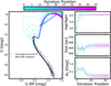 |
Fig. 3 Convergence of the iterative fitting loop (see Fig. 1) for M67 (NGC 2682). Left panel: PARSEC isochrone fits to the observed CMD for each iteration. Right panels: variation in the cluster parameters in the iterations before they converged in the first round at the 45th iteration. |
4 Performance for simulated clusters
4.1 Cluster simulations
We tested the performance of our method on simulated star clusters with controlled binary properties and typical Gaia DR3-like uncertainties. Using PARSEC isochrones 1.2S, we simulated coeval chemically homogeneous stellar populations of 500 cluster members with primary masses randomly sampled from a Kroupa IMF (with a lower mass bound of 0.1 M⊙; Kroupa 2001). The probability of a star being in a binary system was governed by Eq. (1), and the corresponding secondary masses of these systems were simulated by randomly sampling mass ratios from a uniform distribution between  and 1.0. The combined flux of each binary system was used to compute the absolute magnitude before we placed the simulated star cluster at a particular distance with an associated line-of-sight extinction to obtain the desired observables for each star. We emphasise that even though we simulated typical Gaia DR3-like uncertainties in the observables, these simulated clusters still represented an idealised scenario because we did not model stellar rotation and differential extinction, both of which affect the position of a star in the CMD (Platais et al. 2012). Moreover, we did not try to model potential systematic errors in the synthetic photometry of PARSEC models either (e.g. Brandner et al. 2023).
4.2 Joint MA-q posteriors for the simulated clusters
As an example, we show in Fig. 4 the recovered values of the masses and mass ratios of individual stars in a simulated cluster based on multi-band photometry along with the Gaia parallax for two cases: a) before (top, shaded) and b) after (bottom) applying Gaussian priors in cluster parameters. The one-to-one comparison plots are significantly improved when we used the cluster parameter information to obtain the weighted MA and q posteriors, and the precision, depicted by the colour of each point, is also improved by almost an order of magnitude. This shows that incorporating this information for the host cluster not only helps us to reduce the degeneracies, but also constrains the location of the single star MS on the CMD. The top panel of this figure indicates that when stars are treated as part of the field, the masses and mass ratios are significantly uncertain. In contrast, the bottom panel shows that the masses of stars are reliably predicted across a wide range of evolutionary phases by the mode of the posterior distribution weighted by the cluster parameter priors. We cannot satisfactorily recover the mass ratios for stars not on the MS or fainter than G = 19 mag (indicated by small black points in the plot), however, because the light ratio in the case of a MS giant binary system is low or the uncertainties in the observables for faint stars are high (see Appendix D). The box in the bottom right panel of Fig. 4 shows a few simulated binary systems with relatively low mass ratios that are predicted to be single stars. This is also the case for the stars that were simulated to be single, but were predicted to be unresolved binaries with intermediate mass ratios. Thus, this depicts the limited mass-ratio sensitivity of our method and that we can reliably predict the mass ratios for only certain unresolved binaries with qtrue above a certain threshold, say qthresh. We computed this optimal qthresh using the receiver operating characteristic curve (ROC), assuming that we can only detect binaries with q > 0.2, and we indicate this by the black dashed line in the figure. This mass-ratio threshold, qthresh, therefore depends on the cluster parameters and the observables used to obtain the posteriors9. A detailed analysis of the completeness and contamination for a sample of simulated clusters is provided in Appendix D.2, along with the efficacy of our iterative approach in Appendix D.1. Further, we investigate the variation in q residuals and uncertainties with magnitude and the simulated mass ratio in Appendix D.3.
5 Results for Gaia DR3 clusters
We applied our method of obtaining the joint posterior distributions of six astrophysical model parameters for each subset of the member stars described in Fig. A.1 of 42 OCs with decent-quality CMDs for which our method was able to predict good cluster parameters that were well suited for characterising unresolved binaries. The membership lists of the 42 OCs comprise 28 073 stars, and posterior samples could not be obtained for 58 of these (because the GBP flux is overestimated in faint sources; Riello et al. 2021), while 814 were flagged as photometric outliers (Sect. 3.3). The typical statistical uncertainties for the remaining 27 201 members are 0.08 in q and 0.01 M⊙ in MA. Since each cluster has a different range of inferred stellar masses and mass ratios (see Table F.1), it is difficult to homogenise the analysis and perform a population study for several clusters. Therefore, we provide a case study of two clusters, NGC 2360 and NGC 2682 (M67), before we compare our results with the literature. A more detailed analysis of the MA-q distribution in cluster population is planned for a future study. The complete versions of Tables F.1 and F.2 that contain the inferred parameters for the 42 OCs and the results for individual member stars are available via the CDS.
5.1 Examples: NGC 2360 and NGC 2682
Figure 5 shows the CMDs of the two clusters with each star coloured by masses (top left) and mass ratios (bottom left), along with their corresponding uncertainties (right panels). The solid black line is the PARSEC 1.2S isochrone corresponding to the estimated cluster parameters (provided on top of each subplot). For NGC 2360, most of the stars that are classified as photometric outliers (shown by red crosses) are likely field star interlopers, while for M67, these are mostly white dwarfs (WDs), blue stragglers, WD-MS binaries, or faint stars with poor GBP photometry. Since modelling all these stellar populations in our simulation dataset is beyond the scope of this work, we only used the q estimates of the MS stars in the grey shaded region. Notably, the uncertainties in the mass ratios increase significantly for stars close to the MSTO, which can be attributed to the increasing difficulty in distinguishing the single star and binary sequences with increasing primary mass where the two sequences intersect near the MSTO (Hurley & Tout 1998; see also Fig. D.3).
Through comparison with the simulated clusters, we obtained the mass-ratio threshold when we used at least either the 2MASS or WISE photometry along with Gaia, qthresh;Gaia+ as 0.34 and 0.25 for NGC 2360 and M67 , respectively. On the other hand, the threshold for Gaia photometry alone, qthresh;Gaia, is similar for both clusters (0.55 and 0.56, respectively). This demonstrates that using multi-band photometry (especially in the near-/mid-infrared) lowers the detection threshold of unresolved binaries, although the degree of improvement in the detection capability varies across clusters.
Figure 6 plots the variation in the binary fraction with MA and the radial distance (adopted from HR24) from the centre. The binary fraction in NGC 2360 increases monotonically for stars with masses higher than ~0.6 M⊙, similar to the trend observed in the Galactic field star population (Offner et al. 2023). In contrast, M67 shows noticeable dips in the binary fraction at about 0.6 and 0.9 M⊙. This variation was also observed in previous studies, such as Childs & Geller (2025). While these fluctuations may not be statistically significant (only at the ~1.5σ level), their origin is likely related to the previously observed gaps in the MS of OCs (Balaguer-Núñez et al. 2005). The right panel of Fig. 6 shows the declining binary fractions with increasing radial distance from the cluster centre. This trend has been reported in several clusters (Dalessandro et al. 2011; Giesers et al. 2019; Zwicker et al. 2024) and is an expected consequence of mass segregation (binaries tend to be more massive than single stars).
To compare the mass-ratio distributions of the two clusters, we only considered the primary masses in the common mass range of 0.49-1.2 M⊙ (shaded area in Fig. 6) and plot their massratio distributions in Fig. 7. The grey shaded regions represent the mass-ratio bins below qthresh;Gaia and are likely to be incomplete. The two distributions are very similar (all bins with q > 0.4 are compatible within 1σ) and exhibit a slight deficiency in the equal-mass binaries. This contrasts with observational studies of field binaries, which typically report an excess of equal-mass twin systems (q ≈ 1; Lucy & Ricco 1979; Tokovinin 2000; El-Badry et al. 2019; Offner et al. 2023). Fig. D.3 shows that this discrepancy likely arises because the mode of the q posterior distribution, truncated at q = 1.0, is systematically biased towards lower values. Furthermore, the degeneracy between MA and q for high mass-ratio systems (see Fig. 1 of Wallace 2024) can also introduce additional biases in our q estimates. Since we did not impose any prior on the mass function that might partially alleviate this degeneracy, the apparent suppression of equal-mass binaries in our results is most likely a methodological artefact and not a physical effect. We discuss some implications of this in Sect. 7 and Appendix D.3. The binary fractions for q ≥ qthresh;Gaia+ and qthresh;Gaia obtained as nbinaries(q ≥ qthresh)/nMS for the two clusters are shown in the red and the blue boxes, respectively, where the uncertainties are estimated as Poisson errors, that is,  , with nMS denoting the number of MS stars in a particular mass bin.
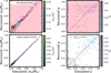 |
Fig. 4 Recovered masses and mass ratios of stars in a simulated solar metallicity cluster (d = 1 kpc, AV ~ 0.1 mag, and log(Age) = 9.5 dex). The modes of the unweighted (top) and weighted (bottom), using cluster parameter information, MA and q posteriors are shown with respect to the simulated parameters. The colour of each data point represents the (fractional) uncertainty in the corresponding (MA) q, and the black data points correspond to stars that are not on the MS or have G ≥ 19 mag. The dashed line in the bottom right panel indicates the qthresh (see text for details) above which we can reliably predict the mass ratio of an unresolved binary in this cluster. |
5.2 Unresolved binary fractions of the 42 OCs
Since our 42 analysed clusters have significantly different massratio thresholds that range from 0.2 to 0.56, we only considered binaries with mass ratios greater than 0.6 in order to minimise the incompleteness effects in studying the dependence of the binary fractions on the fundamental cluster parameters such as age, metallicity, and distance. Figure 8 shows these trends where the data points are coloured according to the mean mass of the MS cluster members. The corresponding Kendall correlation matrix is shown in Fig. E.2. The high mass-ratio binary fraction is correlated with the cluster ages, but correlates only weakly and is anti-correlated with distance and metallicity. The correlation with the cluster age can be interpreted as a result of mass segregation and selective mass loss in the form of low-mass stars, which are less likely to host binary companions (Moe & Di Stefano 2017; Winters et al. 2019), thereby resulting in an increase in the fraction of stars in binary systems over time. The trend with the distance is also expected because more close binaries remain unresolved by Gaia at larger distances (e.g. Donada et al. 2023). This is also consistent with the fact that we can only observe the brighter portion of the MS of distant clusters, thus mirroring the observed trend of increasing binary fraction with the mass of the primary star (Figs. 9, and E.2). Furthermore, the high mass-ratio binary fraction weakly declines with the cluster metallicity, which agrees with the literature (e.g. Gao et al. 2017; Moe et al. 2019; Donada et al. 2023) but might also be explained by the apparent weak anti-correlation in metallicity with the distance for our sample of OCs (see Fig. E.2). Therefore, a wider coverage in metallicity is required for clusters at similar ages and distances to corroborate this correlation.
Another trend that is widely studied, especially in the case of field star population, is the variation in the binary fraction with the primary stellar mass (e.g. Li et al. 2022; Offner et al. 2023). We explore this in Fig. 9 by plotting the unresolved binary fraction for all detected and for only high mass-ratio binaries (q ≥ 0.6) in red and blue, respectively, where each mass bin contains about 1400 MS stars. We also overplot the fit proposed by Arenou (2011, our Eq. (1)) to the observed trend in the field star population. The fit for the Galactic field agrees well with our results for all detected binaries in OCs, specifically for stars with masses higher than 0.6 M⊙ (unshaded region in the plot). In addition, the high mass-ratio binary fraction increases monotonically with the stellar mass for a similar mass range. However, the apparent decline in the binary fraction for 0.5-0.6 M⊙10 and an excess of binaries for lower stellar masses in both cases might be due to the well-known deviations of theoretical isochrones with observations at the low-mass regime (e.g. Bell et al. 2014; Fritzewski et al. 2019; Brandner et al. 2023; Wang et al. 2025). In these cases, the modelled isochrone tends to be bluer (redder) than the observations, thereby resulting in a higher (lower) inferred binary fraction among low-mass stars (this is the case for NGC 2287 and NGC 3532 in particular). As mentioned in Sects. 3.2 and 4, we did not model this effect in our simulations, and therefore, the binary fraction estimates in this mass regime might be biased. Future improvements to the synthetic photometry through either empirical corrections or better low-mass stellar models are necessary to mitigate this discrepancy and improve the reliability of the binary identification in the low-mass regime.
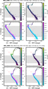 |
Fig. 5 Colour-magnitude diagrams of NGC 2360 (top) and NGC 2682 (M67; bottom). For each cluster, the CMDs are coloured by the primary masses and mass ratios (left) and the corresponding uncertainties (right). The identified photometric outliers are shown by red crosses, and the grey shaded region encloses the MS stars with G ≤ 19 mag. The inferred cluster parameters, along with the spectroscopic metallicity, are listed at the top of each panel. |
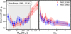 |
Fig. 6 Variation in the unresolved binary fraction with the primary mass (left) and with the radial distance (adopted from HR24) from the cluster centre in units of rc (right). The grey shaded region enclosed by the dashed vertical lines indicates the mass range in common between the two clusters. |
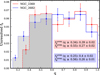 |
Fig. 7 q distributions of the detected unresolved binaries (in the mass range of 0.49-1.2 M⊙) in NGC 2360 and NGC 2682 (M67) shown by red and blue lines, respectively. The grey shaded region indicates the mass-ratio bins below qthresh;Gaia, and the estimated binary fractions for the two mass-ratio thresholds, i.e. qthresh;Gaia and qthresh;Gaia+, are reported along with the Poisson uncertainties. |
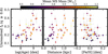 |
Fig. 8 Dependence of the unresolved binary fraction with a high mass ratio (q ≥ 0.6), fb, with the cluster-wide parameters, i.e. log(Age) (left), distance (middle), and [Fe/H] (right) for the 42 OCs. The data points are coloured by the mean mass of MS primary stars. The grey error bars represent the Poisson uncertainties in the binary fractions and 1σ errors in the cluster parameters. |
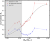 |
Fig. 9 Variation in the unresolved binary fraction with the mass of the primary star for all detected binaries (red) and for high mass-ratio binaries alone (q ≥ 0.6; blue). The fit provided by Arenou (2011), our Eq. (1), to the observed variation in the field is overplotted by the dashed black line. The shaded region corresponds to the masses ≤0.6M⊙, wherein the binary fractions are expected to be spuriously inflated due to colour deviations of the observed Gaia DR3 photometry from the PARSEC isochrones. |
6 Comparison with the literature
6.1 Stellar masses
Figure 10 compares the total mass of unresolved binary systems with the stellar masses provided by HR24, Khalatyan et al. (2024), and Almeida et al. (2023, hereafter AMD23). HR24 and Khalatyan et al. (2024) used general-purpose approaches that did not take the stellar multiplicity into account. HR24 used the G magnitude, along with the GBP – GRP colour indices for old clusters, to estimate stellar masses from PARSEC isochrones after previously determining age, distance, and extinction, and assuming solar metallicity. Khalatyan et al. (2024) trained the extreme gradient-boosted tree system, xgboost (Chen & Guestrin 2016), on ground-based spectroscopic surveys (Queiroz et al. 2023) to predict stellar masses of all ∼220 million Gaia DR3 stars with low-resolution BP/RP spectra (De Angeli et al. 2023), most of which are field stars. In contrast, AMD23 specifically focused on OCs including unresolved binaries: they estimated the individual stellar masses in a Monte Carlo framework while comparing observed and simulated clusters, where the synthetic photometry was generated from PARSEC stellar models. Figure 10 shows that our masses for the single-star systems agree well with the literature, with the total mass of binary systems lying within the region enclosed by blue (dashed) and red (solid) lines, indicating q = 1 and q = 0, respectively. The exception is the case of BH 99 stellar masses reported by AMD23 in panel (c) of the figure, shown by the pink data points. No such discrepancy is detected for the BH 99 cluster members in comparison with HR24 and Khalatyan et al. (2024), and we therefore conclude that this is the result of an inconsistency in the AMD23 masses for this cluster, and consequently its mass ratios. We therefore removed it from the subsequent analysis. The comparison of the total stellar masses with AMD23 in panel (d) shows that the two studies agree in general, with a median fractional absolute difference of  .
.
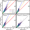 |
Fig. 10 Comparison of the total mass of unresolved binaries with the stellar masses of the cluster members provided in the literature. (a) HR24; (b) Khalatyan et al. (2024); (c and d) Individual and total stellar masses i.e. including the masses of companions provided by AMD23. The red (solid), orange (dash-dotted) and the blue (dashed) lines indicate the q = 0, q = 0.5 and q = 1 relations, respectively. The dashed black line in panel (d) is the one-to-one line, and the pink circles in panel (c) are the inconsistent AMD23 stellar masses reported for BH 99 members (see text for details). |
6.2 Binary mass ratios and binary fractions
Figure 11 compares our predicted mass ratios with those by AMD23 and Childs & Geller (2025, hereafter Childs25) for 30 (8342 members) and 7 (4890 members) overlapping OCs, respectively. The common low mass ratio (q ≤ 0.5) region is shaded grey because the reliability of comparisons between different studies diminishes in this low-q regime (e.g. Childs25 found that their mass ratios are only reliable for q > 0.5). Our predictions and previous studies agree well, with a few ambiguously classified binaries and singles compared to AMD23, and our mass ratios are typically higher by 0.1 than those of Childs25. While AMD23 only relied on the Gaia DR2 photometry, we used the multi-band photometry including the near-and mid-infrared, which led to a better identification of lower-q unresolved binaries. The differences in our comparison with Childs25 are correlated with offsets in the metallicity (our study adopted spectroscopic [Fe/H] values from the literature, whereas Childs25 inferred [Fe/H] from cluster CMDs) and derived extinctions. Figure D.4 shows that an offset of about 0.1 dex in [Fe/H] and 0.1 mag in AV can result in significant differences in the predicted mass ratios. A different photometric survey of Pan-STARRS1 used by Childs25, in contrast to the WISE survey we used might also contribute to minor differences in the predicted mass ratios. Nevertheless, we show that our predicted mass ratios agree well when compared to the direct observations of SB2 binaries in M67 and NGC 2516 in Fig. E.3, taken from Geller et al. (2021) and Lipartito et al. (2021), respectively (cross-matched within 0.5"), where our mass-ratio predictions are slightly underestimated by a median absolute offset of 0.049 for M67 members.
The comparison of the recovered high-q unresolved binary fractions with a few previous studies (Donada et al. 2023; Cordoni et al. 2023; AMD23; Childs25) is shown in Fig. 12, considering the overlapping stellar mass range, wherever these data are available. Our binary fractions are in general slightly higher (by a factor of ~1.4) than those of other studies, which, except for Childs25, only used the Gaia photometry. A wider wavelength range while including infrared photometry along with the measurements in the optical band has been shown to result in a better detection rate of unresolved binaries in comparison to optical photometry (e.g. Steele et al. 2011; Malofeeva et al. 2022). However, binary fractions larger than those reported by Childs25 might arise from differences in the membership lists and the slightly higher mass ratios predicted by our method than in BASE-9 (Robinson et al. 2016), which was used by Childs25.
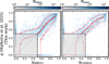 |
Fig. 11 Comparison of the predicted mass ratios with estimates by AMD23 (left) and Childs25 (right). The shaded region indicates the low-q region, and the solid and dashed red lines denote the running median and the 16th to 84th percentiles, respectively. |
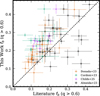 |
Fig. 12 Comparison of high mass-ratio (q > 0.6) binary fractions with the literature while using the same mass range, when available. |
6.3 Fundamental cluster parameters
Finally, we compare our inferred cluster parameters (log(Age), distance, and AV) with some well-known cluster census studies (Bossini et al. 2019; Cantat-Gaudin et al. 2020; Dias et al. 2021; Hunt & Reffert 2023; Cavallo et al. 2024) in Fig. 13. Our results broadly agree overall with previous studies, with a few deviations in the ages of young OCs and in the distance estimates of OCs that lie farther away. Only the AV values display larger offsets relative to the estimates of Hunt & Reffert (2023) and Cavallo et al. (2024). We attribute this to the inclusion of infrared photometry in our analysis, which helps to partially break the age-extinction degeneracy, which is a common limitation in isochrone fitting methods. The typical offsets in comparison to Bossini et al. (2019); Cantat-Gaudin et al. (2020); Dias et al. (2021) are  for log(Age),
  for the distance, and
  for AV. The ages of some well-known young OCs, such as Blanco 1, are slightly overestimated by 0.20.4 dex, but we show in Fig. D.4 that this offset in the OC age does not significantly affect our inferred primary stellar masses and mass ratios.
7 Discussion
We have introduced a new, fast strategy for characterising unresolved binaries in OCs using Simulation-Based Inference (SBI) while simultaneously fitting for the fundamental cluster parameters. We successfully applied our method to a sample of 42 OCs yielding typical uncertainties of 0.08 in q and 0.01 M⊙ (or 1%) in MA. The principal objectives of this study were to (i) explore the trends of binary fraction variation in different clusters, (ii) compare the binary stellar population in the OCs with that in the Galactic field, and (iii) provide a critical assessment of the performance and limitations of our method. We expand on our findings and place them in a broader context in the following sections.
7.1 Binary fraction trends. Dependence on age and [Fe/H]
The dependence of the binary fraction in the Galactic field and in open clusters on age and metallicity has been explored extensively in previous studies (e.g., El-Badry & Rix 2019; Niu et al. 2020; Hwang et al. 2021; Donada et al. 2023; Pang et al. 2023; Alexander & Albrow 2025). Figure 8 shows that the fraction of unresolved binaries in OCs with a high mass ratio tends to increase with age. This trend has been reported before (Jadhav et al. 2021; Donada et al. 2023; Childs & Geller 2025), specifically, for cluster cores by Cordoni et al. (2023), whose findings also reflect the effects of mass segregation. While Niu et al. (2020) did not identify a clear correlation, they suggested that clusters with larger evolutionary parameters might exhibit higher binary fractions. Conversely, Pang et al. (2023) and Thompson et al. (2021) reported a declining trend in the overall binary fraction with cluster age. Specifically, Pang et al. (2023), selected binaries with q > 0.4 and used a ridge-line method, based on which, they noted a modest increase for older clusters beyond 100 Myr, whereas Thompson et al. (2021), based on a sample of only eight OCs, reported that the binary fraction decreased during the first 200 Myr and became constant for older OCs. Based on a probabilistic generative modelling approach, Alexander & Albrow (2025) reported a decline in the binary fraction with cluster age. The N-body simulations by Portegies Zwart et al. (2001) and Fregeau et al. (2009) suggested, however, that the initial decrease arises from the destruction of soft binaries, while a subsequent increase in binary fraction occurs due to the preferential evaporation of low-mass single stars. Considering that most of the clusters in our sample are older than 100 Myr, the observed increase in high mass-ratio binary fraction is likely a consequence of the latter process while confirming the early-phase decline in binary fraction predicted by simulations would require a larger sample of younger OCs.
With regard to the metallicity dependence of binary fraction, previous studies (Grether & Lineweaver 2007; Yuan et al. 2015; Badenes et al. 2018; Moe et al. 2019; Mazzola et al. 2020) have reported an anti-correlation for close binaries in the field star population. El-Badry & Rix (2019) further found that this anticorrelation only emerges for binaries with separations ≲200 AU. While studying wide binaries using metallicities from LAMOST and Gaia astrometry, Hwang et al. (2021) observed that the fraction of wide binaries first increases with metallicity and peaks close to [Fe/H] ~ 0 dex, along with a sharp decline for higher metallicities. Since the wide binary population is rare in large OCs (Scally et al. 1999; Parker et al. 2009; Deacon & Kraus 2020; Rozner & Perets 2023; Cournoyer-Cloutier et al. 2024), we can expect differences in their results and in the right panel of Fig. 8. Given that OCs probe a smaller metallicity range than field stars (Spina et al. 2022), previous studies (e.g. Donada et al. 2023; Cordoni et al. 2023; Childs et al. 2024) only reported a weak or absent correlation with the metallicity. Similar conclusions were also drawn for globular clusters (Milone et al. 2012; Ji & Bregman 2015). Although a declining trend of the binary fraction with OC metallicity is observed in Fig. 8, sample selection effects (see Fig. E.2) make it difficult to robustly establish this dependence. A larger sample including metal-poor OCs would be useful to constrain this correlation better.
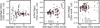 |
Fig. 13 Comparison of the cluster parameters with the literature. The coloured data points denote the estimates from Bossini et al. 2019; Cantat-Gaudin et al. 2020; Dias et al. 2021, and the grey circles indicate the parameters inferred by Hunt & Reffert 2023 and Cavallo et al. 2024. The dashed red line indicates the line of ideal agreement. |
7.2 Binary fractions in OCs distinct from those in the Galactic field?
Binary fractions of main-sequence stars, particularly FGK-type stars, have been found to be broadly consistent with those observed in OCs (Bouvier et al. 1997; Patience et al. 2002; Deacon & Kraus 2020; Torres et al. 2021). Recent studies (Jadhav et al. 2021; Cordoni et al. 2023; Childs25) have investigated the dependence of multiplicity on the primary mass using Gaia DR2/DR3 OC data. Cordoni et al. (2023) reported that the binary fraction distribution of 72 out of 78 OCs was relatively flat with stellar mass. In contrast, Jadhav et al. (2021) and Childs25 reported a strong positive correlation between the binary fraction and primary mass for stars ≳0.7 M⊙, while lowermass stars exhibit a declining trend, which Childs25 attributed to an increased field star contamination. In Fig. 9, we combined all members of our 42 OCs to examine the global distribution of binary stars with the primary stellar mass. For stars with masses higher than 0.6 M⊙, the observed distribution agrees well with trends in the field population, whereas a higher multiplicity rate is observed among the lower masses. We attribute this primarily to the known discrepancies in PARSEC isochrones in the low-mass regime (Wang et al. 2025), where bluer isochrones can artificially increase the inferred unresolved binary fraction, while significant field star contamination is unlikely given our adopted G-band magnitude cut of ≲19 mag. Nevertheless, other explanations for the observed excess in low-mass binaries are also possible. One is that low-mass stars preferentially occur in high mass-ratio systems (e.g. Goodwin 2013), though opposing evidence has been reported (Duchêne & Kraus 2013). Another possibility, supported by N-body simulations (e.g. Portegies Zwart et al. 2001; de la Fuente Marcos & de la Fuente Marcos 2010), is the preferential loss of single low-mass stars, which can produce an apparent increase in the cluster binary fraction both with age (Fig. 8, Sect. 7.1) and within the low-mass bin dominated by M-type stars. Resolving these effects in detail will require improved theoretical isochrone models in the low-mass regime and larger samples of OCs.
In summary, taking into account the evidence that most stars in the Galaxy form in compact aggregates (Lada & Lada 2003; Quintana et al. 2025), even though most of them dissolve very quickly (Lamers et al. 2005; Anders et al. 2021), our analysis suggests that there are similarities among the binary stellar populations in OCs and the Galactic field. The literature shows, however, that the differences in the separation distributions cannot be explained without the production of wide binaries in isolated star formation (Parker et al. 2009) or a huge contribution from small clusters, in which wide binaries have been shown to have higher survival rates through N-body simulations (Rozner & Perets 2023).
7.3 Method performance and scope
Our predicted primary stellar masses agree very well with previous studies and depict that, as expected, a significant fraction of the 200 million stars analysed by Khalatyan et al. (2024) are unresolved binaries. Depending on the light ratio, treating a binary system as a single star can strongly bias the derived stellar parameters, in particular, stellar masses (e.g. El-Badry et al. 2018; Anders et al. 2022 Appendix D; AMD23). This highlights the importance of accounting for the presence of binary companions in future analyses to obtain more accurate stellar parameters. Figure E.1 serves as one such illustration in which the assumption of only single stars can lead to a markedly different interpretation of the dynamical state of a cluster.
With respect to computational cost, our method, once trained, is very fast compared to previous MCMC methods employed by AMD23 and Childs25. Using SBI, we were able to obtain 20 000 posterior samples for model parameters within 2 to 3 seconds on a single core for one star, while each iteration in the cluster parameter estimation loop takes about 8 seconds for a cluster with about 1800 member stars running on seven cores. Moreover, as shown in depth in Sect. 4 and Appendix D, our method produces competitive estimates for masses and mass ratios while inferring well-fitted isochrones to the observed CMD.
Nevertheless, there are still some limitations to our method. (i) The cluster parameter fitting iterative loop can struggle to estimate the parameters of young OCs and those affected by differential extinction, (ii) the degeneracy in MA and q along with the mode of q posterior biased towards lower values in the high-q regime can result in some underestimated mass ratios of nearly equal-mass binaries, (iii) systematics in the stellar models (specifically for low-mass stars) likely result in an unreliable characterisation of low-mass binaries, and (iv) triple and higher-order systems are not taken into account. We plan to implement future improvements in our iterative cluster parameter fitting loop to also include some of the other clusters that were classified as good or poor in the study of characterisation of unresolved binaries. The mass-q degeneracy can probably be addressed by adding a prior on the mass function in OCs. However, we refrain from applying such a prior in this first study because of the limited understanding of how the mass-function prior might influence the estimated total OC mass, which is beyond the scope of this work.
8 Conclusions
We have outlined a new and efficient method for detecting and characterising unresolved binaries in open clusters while simultaneously deriving optimal cluster parameters. The method combines multi-band photometry from Gaia, 2MASS, and WISE with Gaia parallaxes to infer posterior distributions of primary mass, mass ratio, metallicity, age, distance, and line-of-sight extinction for individual stars using Simulation-Based Inference (SBI). Using an iterative framework to select member stars by their evolutionary phases, we robustly estimated the global cluster parameters while keeping the metallicity fixed to a spectroscopic estimate obtained from the literature.
From custom cluster simulations, we found that we reliably detected unresolved binaries in OCs above mass-ratio thresholds ranging from qthresh ~ 0.2-0.56, depending on the cluster properties and the set of available observables. Analysing two example OCs, NGC 2360 and NGC 2682 (M67), we found that the binary fraction in NGC 2360 increases monotonically for masses ≳0.6 M⊙, whereas M67 exhibits a number of dips, most likely due to gaps in the MS. We confirmed that both clusters show higher binary fractions in the cluster cores.
With this paper, we publish the results for 42 OCs for which our method works most successfully (OCs with clean and well-fitted CMDs suitable for studying their binary stellar populations) and provide a catalogue of individual stellar masses and mass ratios for 27 201 member stars with typical uncertainties of 0.08 in q and 0.01 M⊙ in MA. An overall analysis of the variation of the unresolved binary fraction with cluster-wide parameters revealed a positive correlation with cluster age and mean primary mass of MS stars and a weak anti-correlation with the cluster metallicity. The dependence of binary fractions on the primary stellar mass, when collating all cluster member stars, demonstrates a similar variation as observed in the Galactic field for stars with masses higher than ≳0.6 M⊙, while lower masses are likely affected by discrepancies in the stellar models we use.
Data availability
Online versions of Tables F.1 and F.2 containing the cluster parameters for the 42 clusters and the results for individual cluster members, respectively, are available at the CDS via https://cdsarc.cds.unistra.fr/viz-bin/cat/J/A+A/706/A62.
Acknowledgements
We thank the anonymous referee for constructive feedback that improved the manuscript. The authors acknowledge all members of the GaiaUB group for insightful discussions throughout the course of this project. This work was (partially) supported by the Spanish MICIN/AEI/10.13039/501100011033 and by “ERDF A way of making Europe” by the European Union through grant PID2021-122842OB-C21 and PID2024-157964OB-C21, and the Institute of Cosmos Sciences University of Barcelona (ICCUB, Unidad de Excelencia María de Maeztu) through grant CEX2024-001451-M and the project 2021-SGR-00679 GRC de l’Agència de Gestió d’Ajuts Universitaris i de Recerca (Generalitat de Catalunya).. This research was partially funded by the Horizon Europe HORIZON-CL4-2023-SPACE-01-71 SPACIOUS project funded under Grant Agreement no. 101135205. FA acknowledges financial support from MCIN/AEI/10.13039/501100011033 through grant RYC2021-03163 8-I, co-funded by European Union NextGenerationEU/PRTR. S. Q. acknowledges support from the National Natural Science Foundation of China (NSFC) through grants 12090040 and 12090042. This work has made use of data from the European Space Agency (ESA) mission Gaia (https://www.cosmos.esa.int/gaia), processed by the Gaia Data Processing and Analysis Consortium (DPAC, https://www.cosmos.esa.int/web/gaia/dpac/consortium). Funding for the DPAC has been provided by national institutions, in particular the institutions participating in the Gaia Multilateral Agreement. This research makes use of public auxiliary data provided by ESA/Gaia/DPAC/CU5 and prepared by Carine Babusiaux.
References
- Alexander, J. S., & Albrow, M. D. 2025, MNRAS, 536, 471 [Google Scholar]
- Allison, R. J., Goodwin, S. P., Parker, R. J., et al. 2009, MNRAS, 395, 1449 [Google Scholar]
- Almeida, A., Monteiro, H., & Dias, W. S. 2023, MNRAS, 525, 2315 [NASA ADS] [CrossRef] [Google Scholar]
- Anders, F., Cantat-Gaudin, T., Quadrino-Lodoso, I., et al. 2021, A&A, 645, L2 [NASA ADS] [CrossRef] [EDP Sciences] [Google Scholar]
- Anders, F., Khalatyan, A., Queiroz, A. B. A., et al. 2022, A&A, 658, A91 [NASA ADS] [CrossRef] [EDP Sciences] [Google Scholar]
- Arenou, F. 2011, in American Institute of Physics Conference Series, 1346, International Workshop on Double and Multiple Stars: Dynamics, Physics, and Instrumentation, eds. J. A. Docobo, V. S. Tamazian, & Y. Y. Balega, 107 [Google Scholar]
- Badenes, C., Mazzola, C., Thompson, T. A., et al. 2018, ApJ, 854, 147 [NASA ADS] [CrossRef] [Google Scholar]
- Balaguer-Núñez, L., Jordi, C., & Galadí-Enríquez, D. 2005, A&A, 437, 457 [NASA ADS] [CrossRef] [EDP Sciences] [Google Scholar]
- Bell, C. P. M., Rees, J. M., Naylor, T., et al. 2014, MNRAS, 445, 3496 [NASA ADS] [CrossRef] [Google Scholar]
- Belokurov, V., Penoyre, Z., Oh, S., et al. 2020, MNRAS, 496, 1922 [Google Scholar]
- Bettis, C. 1977, ApJ, 214, 106 [Google Scholar]
- Bossini, D., Vallenari, A., Bragaglia, A., et al. 2019, A&A, 623, A108 [NASA ADS] [CrossRef] [EDP Sciences] [Google Scholar]
- Bouvier, J., Rigaut, F., & Nadeau, D. 1997, A&A, 323, 139 [NASA ADS] [Google Scholar]
- Brandner, W., Calissendorff, P., & Kopytova, T. 2023, AJ, 165, 108 [NASA ADS] [CrossRef] [Google Scholar]
- Bressan, A., Marigo, P., Girardi, L., et al. 2012, MNRAS, 427, 127 [NASA ADS] [CrossRef] [Google Scholar]
- Brewer, L. N., Sandquist, E. L., Mathieu, R. D., et al. 2016, AJ, 151, 66 [NASA ADS] [CrossRef] [Google Scholar]
- Brogaard, K., Grundahl, F., Sandquist, E. L., et al. 2021, A&A, 649, A178 [NASA ADS] [CrossRef] [EDP Sciences] [Google Scholar]
- Cantat-Gaudin, T., Anders, F., Castro-Ginard, A., et al. 2020, A&A, 640, A1 [NASA ADS] [CrossRef] [EDP Sciences] [Google Scholar]
- Castro-Ginard, A., McMillan, P. J., Luri, X., et al. 2021, A&A, 652, A162 [NASA ADS] [CrossRef] [EDP Sciences] [Google Scholar]
- Castro-Ginard, A., Penoyre, Z., Casey, A. R., et al. 2024, A&A, 688, A1 [NASA ADS] [CrossRef] [EDP Sciences] [Google Scholar]
- Cavallo, L., Spina, L., Carraro, G., et al. 2024, AJ, 167, 12 [NASA ADS] [CrossRef] [Google Scholar]
- Chen, T., & Guestrin, C. 2016, in Proceedings of the 22nd ACM SIGKDD International Conference on Knowledge Discovery and Data Mining, KDD ’16 (ACM), 785 [Google Scholar]
- Childs, A. C., & Geller, A. M. 2025, ApJ, 989, 104 [Google Scholar]
- Childs, A. C., Geller, A. M., von Hippel, T., Motherway, E., & Zwicker, C. 2024, ApJ, 962, 41 [Google Scholar]
- Choi, J., Dotter, A., Conroy, C., et al. 2016, ApJ, 823, 102 [Google Scholar]
- Cohen, R. E., Geller, A. M., & von Hippel, T. 2020, AJ, 159, 11 [Google Scholar]
- Cordoni, G., Milone, A. P., Marino, A. F., et al. 2023, A&A, 672, A29 [NASA ADS] [CrossRef] [EDP Sciences] [Google Scholar]
- Cournoyer-Cloutier, C., Tran, A., Lewis, S., et al. 2021, MNRAS, 501, 4464 [NASA ADS] [CrossRef] [Google Scholar]
- Cournoyer-Cloutier, C., Sills, A., Harris, W. E., et al. 2024, ApJ, 977, 203 [Google Scholar]
- Cranmer, K., Brehmer, J., & Louppe, G. 2020, PNAS, 117, 30055 [NASA ADS] [CrossRef] [Google Scholar]
- Dalessandro, E., Lanzoni, B., Beccari, G., et al. 2011, ApJ, 743, 11 [Google Scholar]
- Danielski, C., Babusiaux, C., Ruiz-Dern, L., Sartoretti, P., & Arenou, F. 2018, A&A, 614, A19 [NASA ADS] [CrossRef] [EDP Sciences] [Google Scholar]
- De Angeli, F., Weiler, M., Montegriffo, P., et al. 2023, A&A, 674, A2 [NASA ADS] [CrossRef] [EDP Sciences] [Google Scholar]
- de la Fuente Marcos, R., & de la Fuente Marcos, C. 2010, ApJ, 719, 104 [CrossRef] [Google Scholar]
- Deacon, N. R., & Kraus, A. L. 2020, MNRAS, 496, 5176 [NASA ADS] [CrossRef] [Google Scholar]
- Dias, W. S., Monteiro, H., Moitinho, A., et al. 2021, MNRAS, 504, 356 [NASA ADS] [CrossRef] [Google Scholar]
- Donada, J., Anders, F., Jordi, C., et al. 2023, A&A, 675, A89 [NASA ADS] [CrossRef] [EDP Sciences] [Google Scholar]
- Dotter, A. 2016, ApJS, 222, 8 [Google Scholar]
- Duchêne, G., & Kraus, A. 2013, ARA&A, 51, 269 [Google Scholar]
- Duquennoy, A., & Mayor, M. 1991, A&A, 248, 485 [NASA ADS] [Google Scholar]
- Ebrahimi, H., Sollima, A., & Haghi, H. 2022, MNRAS, 516, 5637 [NASA ADS] [CrossRef] [Google Scholar]
- El-Badry, K., & Rix, H.-W. 2019, MNRAS, 482, L139 [NASA ADS] [Google Scholar]
- El-Badry, K., Rix, H.-W., Ting, Y.-S., et al. 2018, MNRAS, 473, 5043 [Google Scholar]
- El-Badry, K., Rix, H.-W., Tian, H., Duchêne, G., & Moe, M. 2019, MNRAS, 489, 5822 [NASA ADS] [CrossRef] [Google Scholar]
- Fabricius, C., Luri, X., Arenou, F., et al. 2021, A&A, 649, A5 [NASA ADS] [CrossRef] [EDP Sciences] [Google Scholar]
- Freedman, D. A., & Diaconis, P. 1981, Zeitsch. Wahrscheinlich. Verwandte Gebiete, 57, 453 [Google Scholar]
- Fregeau, J. M., Ivanova, N., & Rasio, F. A. 2009, ApJ, 707, 1533 [NASA ADS] [CrossRef] [Google Scholar]
- Fritzewski, D. J., Barnes, S. A., James, D. J., et al. 2019, A&A, 622, A110 [NASA ADS] [CrossRef] [EDP Sciences] [Google Scholar]
- Fuhrmann, K., Chini, R., Kaderhandt, L., & Chen, Z. 2017, ApJ, 836, 139 [Google Scholar]
- Gaia Collaboration (Prusti, T., et al.) 2016, A&A, 595, A1 [NASA ADS] [CrossRef] [EDP Sciences] [Google Scholar]
- Gaia Collaboration (Babusiaux, C., et al.) 2018, A&A, 616, A10 [NASA ADS] [CrossRef] [EDP Sciences] [Google Scholar]
- Gaia Collaboration (Arenou, F., et al.) 2023a, A&A, 674, A34 [CrossRef] [EDP Sciences] [Google Scholar]
- Gaia Collaboration, Vallenari, A., Brown, A. G. A., et al. 2023b, A&A, 674, A1 [NASA ADS] [CrossRef] [EDP Sciences] [Google Scholar]
- Gao, S., Zhao, H., Yang, H., & Gao, R. 2017, MNRAS, 469, L68 [NASA ADS] [CrossRef] [Google Scholar]
- Geller, A. M., de Grijs, R., Li, C., & Hurley, J. R. 2013, ApJ, 779, 30 [NASA ADS] [CrossRef] [Google Scholar]
- Geller, A. M., de Grijs, R., Li, C., & Hurley, J. R. 2015, ApJ, 805, 11 [Google Scholar]
- Geller, A. M., Mathieu, R. D., Latham, D. W., et al. 2021, AJ, 161, 190 [NASA ADS] [CrossRef] [Google Scholar]
- Giesers, B., Kamann, S., Dreizler, S., et al. 2019, A&A, 632, A3 [NASA ADS] [CrossRef] [EDP Sciences] [Google Scholar]
- Goodwin, S. P. 2013, MNRAS, 430, L6 [NASA ADS] [Google Scholar]
- Goodwin, S. P., & Kroupa, P. 2005, A&A, 439, 565 [NASA ADS] [CrossRef] [EDP Sciences] [Google Scholar]
- Greenberg, D., Nonnenmacher, M., & Macke, J. 2019, in Proceedings of Machine Learning Research, 97, Proceedings of the 36th International Conference on Machine Learning, eds. K. Chaudhuri & R. Salakhutdinov (PMLR), 2404 [Google Scholar]
- Grether, D., & Lineweaver, C. H. 2007, ApJ, 669, 1220 [Google Scholar]
- Guszejnov, D., Raju, A. N., Offner, S. S. R., et al. 2023, MNRAS, 518, 4693 [Google Scholar]
- Heggie, D. C. 1975, MNRAS, 173, 729 [NASA ADS] [CrossRef] [Google Scholar]
- Hunt, E. L., & Reffert, S. 2023, A&A, 673, A114 [NASA ADS] [CrossRef] [EDP Sciences] [Google Scholar]
- Hunt, E. L., & Reffert, S. 2024, A&A, 686, A42 [NASA ADS] [CrossRef] [EDP Sciences] [Google Scholar]
- Hurley, J., & Tout, C. A. 1998, MNRAS, 300, 977 [CrossRef] [Google Scholar]
- Hurley, J. R., Pols, O. R., Aarseth, S. J., & Tout, C. A. 2005, MNRAS, 363, 293 [NASA ADS] [CrossRef] [Google Scholar]
- Hurley, J. R., Aarseth, S. J., & Shara, M. M. 2007, ApJ, 665, 707 [NASA ADS] [CrossRef] [Google Scholar]
- Hwang, H.-C., Ting, Y.-S., Schlaufman, K. C., Zakamska, N. L., & Wyse, R. F. G. 2021, MNRAS, 501, 4329 [NASA ADS] [CrossRef] [Google Scholar]
- Ivanova, N., Belczynski, K., Fregeau, J. M., & Rasio, F. A. 2005, MNRAS, 358, 572 [NASA ADS] [CrossRef] [Google Scholar]
- Jadhav, V. V., Roy, K., Joshi, N., & Subramaniam, A. 2021, AJ, 162, 264 [NASA ADS] [CrossRef] [Google Scholar]
- Janes, K., & Adler, D. 1982, ApJS, 49, 425 [Google Scholar]
- Ji, J., & Bregman, J. N. 2015, ApJ, 807, 32 [Google Scholar]
- Jiang, Y., Zhong, J., Qin, S., et al. 2024, ApJ, 971, 71 [NASA ADS] [CrossRef] [Google Scholar]
- Joshi, Y. C., Deepak, & Malhotra, S. 2024, Front. Astron. Space Sci., 11, 1348321 [NASA ADS] [CrossRef] [Google Scholar]
- Kaczmarek, T., Olczak, C., & Pfalzner, S. 2011, A&A, 528, A144 [NASA ADS] [CrossRef] [EDP Sciences] [Google Scholar]
- Kalirai, J. S., & Richer, H. B. 2010, Philos. Trans. Roy. Soc. Lond. Ser. A, 368, 755 [Google Scholar]
- Kamdar, H., Conroy, C., Ting, Y.-S., et al. 2019, ApJ, 884, L42 [NASA ADS] [CrossRef] [Google Scholar]
- Kelly, R. P., Warne, D. J., Frazier, D. T., et al. 2025, arXiv e-prints [arXiv:2503.12315] [Google Scholar]
- Khalatyan, A., Anders, F., Chiappini, C., et al. 2024, A&A, 691, A98 [NASA ADS] [CrossRef] [EDP Sciences] [Google Scholar]
- Kroupa, P. 2001, MNRAS, 322, 231 [NASA ADS] [CrossRef] [Google Scholar]
- Krumholz, M. R., McKee, C. F., & Bland -Hawthorn, J. 2019, ARA&A, 57, 227 [Google Scholar]
- Kruskal, J. B. 1956, Proc. Am. Math. Soc., 7, 48 [CrossRef] [Google Scholar]
- Lada, C. J., & Lada, E. A. 2003, ARA&A, 41, 57 [Google Scholar]
- Lamers, H. J. G. L. M., Gieles, M., Bastian, N., et al. 2005, A&A, 441, 117 [NASA ADS] [CrossRef] [EDP Sciences] [Google Scholar]
- Li, L., Shao, Z., Li, Z.-Z., et al. 2020, ApJ, 901, 49 [Google Scholar]
- Li, J., Li, J., Liu, C., et al. 2022, ApJ, 933, 119 [Google Scholar]
- Li, J., Rix, H.-W., Ting, Y.-S., et al. 2025, A&A, 704, A126 [NASA ADS] [CrossRef] [EDP Sciences] [Google Scholar]
- Lipartito, I., Bailey, III, J. I., Brandt, T. D., et al. 2021, AJ, 162, 285 [Google Scholar]
- Liu, R., Shao, Z., & Li, L. 2025, AJ, 169, 116 [Google Scholar]
- Lucy, L. B., & Ricco, E. 1979, AJ, 84, 401 [NASA ADS] [CrossRef] [Google Scholar]
- Malofeeva, A. A., Seleznev, A. F., & Carraro, G. 2022, AJ, 163, 113 [NASA ADS] [CrossRef] [Google Scholar]
- Malofeeva, A. A., Mikhnevich, V. O., Carraro, G., & Seleznev, A. F. 2023, AJ, 165, 45 [NASA ADS] [CrossRef] [Google Scholar]
- Marks, M., Kroupa, P., & Oh, S. 2011, MNRAS, 417, 1684 [NASA ADS] [CrossRef] [Google Scholar]
- Mazur, B., Krzeminski, W., & Kaluzny, J. 1995, MNRAS, 273, 59 [Google Scholar]
- Mazzola, C. N., Badenes, C., Moe, M., et al. 2020, MNRAS, 499, 1607 [CrossRef] [Google Scholar]
- Mermilliod, J. C., Rosvick, J. M., Duquennoy, A., & Mayor, M. 1992, A&A, 265, 513 [NASA ADS] [Google Scholar]
- Milone, A. P., Piotto, G., Bedin, L. R., et al. 2012, A&A, 540, A16 [NASA ADS] [CrossRef] [EDP Sciences] [Google Scholar]
- Moe, M., & Di Stefano, R. 2017, ApJS, 230, 15 [Google Scholar]
- Moe, M., Kratter, K. M., & Badenes, C. 2019, ApJ, 875, 61 [NASA ADS] [CrossRef] [Google Scholar]
- Niu, H., Wang, J., & Fu, J. 2020, ApJ, 903, 93 [Google Scholar]
- Offner, S. S. R., Moe, M., Kratter, K. M., et al. 2023, in Astronomical Society of the Pacific Conference Series, 534, Protostars and Planets VII, eds. S. Inutsuka, Y. Aikawa, T. Muto, K. Tomida, & M. Tamura, 275 [Google Scholar]
- Pang, X., Wang, Y., Tang, S.-Y., et al. 2023, AJ, 166, 110 [NASA ADS] [CrossRef] [Google Scholar]
- Papamakarios, G., & Murray, I. 2016, in Advances in Neural Information Processing Systems, 29, eds. D. Lee, M. Sugiyama, U. Luxburg, I. Guyon, & R. Garnett (Curran Associates, Inc.) [Google Scholar]
- Papamakarios, G., Nalisnick, E., Rezende, D. J., Mohamed, S., & Lakshmi-narayanan, B. 2021, J. Mach. Learn. Res., 22, 1 [Google Scholar]
- Parker, R. J., Goodwin, S. P., Kroupa, P., & Kouwenhoven, M. B. N. 2009, MNRAS, 397, 1577 [NASA ADS] [CrossRef] [Google Scholar]
- Patience, J., Ghez, A. M., Reid, I. N., & Matthews, K. 2002, AJ, 123, 1570 [NASA ADS] [CrossRef] [Google Scholar]
- Pavlík, V., Davies, M. B., Leitinger, E. I., et al. 2025, A&A, 703, A157 [NASA ADS] [CrossRef] [EDP Sciences] [Google Scholar]
- Platais, I., Melo, C., Quinn, S. N., et al. 2012, ApJ, 751, L8 [NASA ADS] [CrossRef] [Google Scholar]
- Portegies Zwart, S. F., McMillan, S. L. W., Hut, P., & Makino, J. 2001, MNRAS, 321, 199 [Google Scholar]
- Prim, R. C. 1957, Bell Syst. Tech. J., 36, 1389 [NASA ADS] [CrossRef] [Google Scholar]
- Queiroz, A. B. A., Anders, F., Chiappini, C., et al. 2023, A&A, 673, A155 [NASA ADS] [CrossRef] [EDP Sciences] [Google Scholar]
- Quintana, A. L., Hunt, E. L., & Parul, H. 2025, A&A, 701, L2 [NASA ADS] [CrossRef] [EDP Sciences] [Google Scholar]
- Raghavan, D., McAlister, H. A., Henry, T. J., et al. 2010, ApJS, 190, 1 [Google Scholar]
- Rastello, S., Carraro, G., & Capuzzo-Dolcetta, R. 2020, ApJ, 896, 152 [NASA ADS] [CrossRef] [Google Scholar]
- Riello, M., De Angeli, F., Evans, D. W., et al. 2021, A&A, 649, A3 [NASA ADS] [CrossRef] [EDP Sciences] [Google Scholar]
- Robinson, E., von Hippel, T., Stein, N., et al. 2016, BASE-9: Bayesian Analysis for Stellar Evolution with nine variables, Astrophysics Source Code Library [record ascl:1608.007] [Google Scholar]
- Rottensteiner, A., & Meingast, S. 2024, A&A, 690, A16 [NASA ADS] [CrossRef] [EDP Sciences] [Google Scholar]
- Rozner, M., & Perets, H. B. 2023, ApJ, 955, 134 [Google Scholar]
- Scally, A., Clarke, C., & McCaughrean, M. J. 1999, MNRAS, 306, 253 [Google Scholar]
- Schlesinger, B. M. 1975, AJ, 80, 1071 [Google Scholar]
- Skrutskie, M. F., Cutri, R. M., Stiening, R., et al. 2006, AJ, 131, 1163 [NASA ADS] [CrossRef] [Google Scholar]
- Soubiran, C., Cantat-Gaudin, T., Romero-Gómez, M., et al. 2018, A&A, 619, A155 [NASA ADS] [CrossRef] [EDP Sciences] [Google Scholar]
- Spina, L., Magrini, L., & Cunha, K. 2022, Universe, 8, 87 [NASA ADS] [CrossRef] [Google Scholar]
- Steele, P. R., Burleigh, M. R., Dobbie, P. D., et al. 2011, MNRAS, 416, 2768 [NASA ADS] [CrossRef] [Google Scholar]
- Sturges, H. A. 1926, J. Am. Statist. Assoc., 21, 65 [CrossRef] [Google Scholar]
- Thompson, B. A., Frinchaboy, P. M., Spoo, T., & Donor, J. 2021, AJ, 161, 160 [NASA ADS] [CrossRef] [Google Scholar]
- Tokovinin, A. A. 2000, A&A, 360, 997 [NASA ADS] [Google Scholar]
- Torres, G. 2020, ApJ, 901, 91 [Google Scholar]
- Torres, G., Latham, D. W., & Quinn, S. N. 2021, ApJ, 921, 117 [Google Scholar]
- van de Kamp, P. 1968, Leaflet Astron. Soc. Pac., 10, 153 [Google Scholar]
- Wallace, A. L. 2024, MNRAS, 527, 8718 [Google Scholar]
- Wang, F., Fang, M., Fu, X., et al. 2025, ApJ, 979, 92 [Google Scholar]
- Winters, J. G., Henry, T. J., Jao, W.-C., et al. 2019, AJ, 157, 216 [NASA ADS] [CrossRef] [Google Scholar]
- Wright, E. L., Eisenhardt, P. R. M., Mainzer, A. K., et al. 2010, AJ, 140, 1868 [Google Scholar]
- Yuan, H. B., Liu, X. W., & Xiang, M. S. 2013, MNRAS, 430, 2188 [NASA ADS] [CrossRef] [Google Scholar]
- Yuan, H., Liu, X., Xiang, M., et al. 2015, ApJ, 799, 135 [NASA ADS] [CrossRef] [Google Scholar]
- Zwicker, C., Geller, A. M., Childs, A. C., Motherway, E., & von Hippel, T. 2024, ApJ, 967, 44 [Google Scholar]
The multi-band photometric observations are compiled by crossmatching Gaia sources with the 2MASS and WISE catalogues, the details of which are presented in Appendix A.
CST > 5.0; class_50 > 0.5; kind = “o”.
Even though our sample contains two moving groups classified by HR24, we use the term “OCs” in a broader sense.
We assume [M/H] = [Fe/H] throughout this study, which is reasonable for OCs in the solar vicinity.
When the posterior sampling with the full set of available observables failed, we used progressively fewer passbands while only employing Gaia photometry in the last attempt.
Neither the parameters nor the corresponding uncertainties changed by more than 0.1% throughout the last five iterations.
Although it will also depend on MA, we opted to keep things simple.
We note that 90% of the OCs in our sample have their lightest stars (with G ≤ 19 mag) lighter than 0.5M⊙.
Appendix A Cross-match with 2MASS and WISE catalogues
We use the DPAC crossmatch catalogues for 2MASS and allWISE to retrieve the corresponding photometry information for the HR24 OC member stars from the respective survey catalogues. This is accomplished by crossmatching the Gaia source_id column with the crossmatch catalogues and using the corresponding clean_tmass_psc_xsc_oid and allwise_oid columns in the DPAC curated catalogues11 for 2MASS and WISE surveys respectively. Due to different spatial resolutions of the three surveys, it is necessary to filter out the crossmatched sources that might be affected by blending issues due to presence of close neighbours, which might have been unresolved due to poorer effective spatial resolution of one survey. We apply the following quality cuts to only select the crossmatched stars in 2MASS and WISE having good photometry: For 2MASS, the photometric quality flag (ph_qual) is set to "AAA" and "AA**" for WISE since only W1 and W2 are the photometric bands of interest. Additionally, for both 2MASS and WISE, the number_of_mates parameter is set to 0.
Figure A.1 shows the distribution of the apparent G magnitude of the members of the analysed 42 clusters (see Sect. 5) with different coloured histograms representing three subsets of stars based on the availability of good photometry. Therefore, most stars brighter than G ≲ 17 mag have good photometry available from either of the infrared surveys, with Gaia being the dominant source of photometry for fainter stars. We derive one SBI posterior for each subset of member stars.
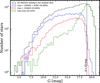 |
Fig. A.1 G mag distribution of HR24 member stars of 42 OCs divided into different sets based on the availability of good photometry (see text for more details) from 2MASS and WISE. The dashed vertical line marks G = 19 mag, beyond which very few stars have good photometric measurements. |
Appendix B Estimation of cluster parameters
We adopt an iterative procedure to estimate the cluster parameters as follows:
We adopt the metallicity estimate from the literature, while for the rest of the parameters we take the mean value of the posterior samples of each star obtained using SBI (Fig. 1) with the resulting mean being considered as the initial guess for that parameter. These cluster parameter priors are then used to assign weights to each posterior sample.
We only select the stars with at least 2% valid samples (samples within 5σ from the mean cluster parameter prior) while keeping the metallicity fixed and do the following:
- (a)
log(Age): Since the age of a cluster is best estimated by the stars near the MSTO, especially for old OCs, we used at least 5 stars near the MSTO and computed the weighted mean and standard deviation (weighted by the individual errors; Soubiran et al. 2018) of their weighted log(Age) modes as the corresponding value for the next iteration. At each iteration, these stars are selected as being the nearest neighbours to the MSTO stars in the theoretical PARSEC isochrones. This is implemented by using the "label" provided with the PARSEC 1.2S isochrones that (approximately) denotes the evolutionary stage of each star. We assign these labels from the theoretical isochrones to the stars in the observed CMD using a nearest-neighbour algorithm and remove any star labelled as a MS or a pre-MS star while estimating the cluster age. Though this selection might not be completely accurate for the first few iterations, it improves significantly during the first 10 iterations (Fig. 3). To also account for the case of young clusters with no or very few evolved stars, we do a check at the 10th iteration if that is the case and proceed to use stars in the upper and lower MS to automate the selection of suitable stars to estimate its age. We only use a vary small fraction of stars in the intermediate portion of the MS (MG ~ 3.0 – 8.0 mag) due to a largely indiscernible nature of isochrones in that region where the cluster ages in range ∼100 – 500 Myr (Rotten-steiner & Meingast 2024) are highly degenerate. We test the robustness of this selection method in Appendix D.1.
- (a)
Distance and extinction: The distance and extinction priors for the next iteration are computed as the weighted mean and standard deviation of the weighted modes of the individual parameter values of each star brighter than G = 18 mag. After 10 iterations we do not include stars significantly displaced from the single star sequence for extinction estimation due to systematically overestimated extinctions for unresolved binaries.
- (a)
At each step, the error in the computed cluster parameter is bounded by a lower value of 0.05 dex for log(Age) and [Fe/H], 0.05 mag for AV and 2% for distance. Although decreasing the lower bound of errors does not lead to significant improvements in the accuracy of the cluster parameters, it results in a large number of stars being classified as outliers due to the absence of a posterior sample within the 5σ of the mean cluster parameter. However, this uncertainty likely represents only a lower bound, as systematic errors arising from the PARSEC stellar models and related factors are expected to dominate the uncertainties in our inferred cluster parameters.
The method is considered to be converged if all the 6 metrics viz., the mean log(Age), distance, and extinction of the OC and their corresponding errors do not change by more than 0.1% in the last 5 iterations. For some OCs, there can be instances where this criteria is not met even though the corresponding isochrones do not visually change over a large number of iterations. To address this, we limit the number of iterations in each round to 50.
We show this automated selection of different stars based on their evolutionary phases for estimation of the cluster parameters at the 1st, 10th, and 45th (i.e. convergence for the first round) in Fig. B.1 for M67 (see also Fig. 3). Furthermore, we test the feasibility of this method on simulated clusters in Fig. D.1.
Appendix C Comparison with conditional sampling of model parameter posteriors with fixed cluster parameters
The SBI package also comes along with a method to sample conditional distributions, i.e. one can provide conditions on a subset of model parameters while sampling the posterior distributions of the rest. However, as previously mentioned in Sect. 3.3, one of the main disadvantages of this method is that it is computationally very expensive along with the limitation that one can only provide delta functions as conditions, thereby rendering this method worthwhile only when the cluster parameters are known a priori with a very high degree of accuracy. Although we see some improvement in the overall accuracy of the masses and mass-ratio estimates in Fig. C.1, we have noted in Fig. 4 that our method can produce satisfactory results at a much lower computational cost without a priori knowledge about the cluster parameters.
Appendix D Performance for simulated clusters: Additional analysis
Appendix D.1 Performance of the iterative cluster parameter estimation method
In this section we test the viability of the iterative cluster parameter estimation method described in Sect. 3.5 for simulated clusters. As mentioned earlier, we kept the metallicity [Fe/H] constant, in this case the true value of the simulated cluster, while iterating through other parameters. We show the comparison of the recovered with the simulated parameters for 24 simulated solar metallicity clusters at 1 kpc in Fig. D.1 wherein one can observe that the method works well for a wide range of cluster parameters. The predicted log(Age) is within ±0.05-0.1 dex of the simulated age of the clusters. On the other hand, the predicted distance is mostly accurate within ±20 pc (2%), whereas the line-of-sight extinction AV is predicted with an accuracy of about 0.08 mag. These are similar to the typical offsets reported in Sect. 6.3 compared to the cluster parameters provided in the literature.
Appendix D.2 Detection efficiency and false positive rate of unresolved binaries above qthresh
In Fig. 4, we observed that our method can lead to a few stars being misclassified as binaries or singles. To see if this false classification is the case for specific stars in the CMD, we consider different bins in the G magnitude, each containing almost similar number of stars. In each bin, we computed the fraction of stars that are falsely predicted as binaries or singles, that is, ffb and ffs, respectively as
 (D.1)
(D.1)
where predicted binaries are stars with  while false binaries are the subset of predicted binaries with qtrue < qthresh and similarly for false singles and true binaries. Figure D.2 shows these fractions for the case of 24 simulated solar metallicity clusters placed at 1 kpc, named as "log(Age)_V", in each G magnitude bin. The gray coloured bins indicate where there were no predicted or true binaries. As one can see, ffb and ffs are mostly lower than 0.2 with a higher false classification rate for stars near the MSTO and those with G mag fainter than 19 mag. This is expected because: a) the single and binary sequences become nearly indistinguishable near the MSTO, and b) there are high uncertainties in the observables for very faint stars, especially the parallax, which becomes significantly uncertain for G ≳ 18 mag (Gaia Collaboration et al. 2023b).
Appendix D.3 q residuals and uncertainties
We assess the recovery of binary mass ratios for correctly identified unresolved binaries in simulated clusters described in Appendix D.5. Figure D.3 shows the residuals in q (defined as recovered minus simulated) and the predicted uncertainties as functions of absolute G magnitude and simulated mass ratio. The solid and dashed lines represent the median and percentile trends, respectively. The median residuals remain negligible across a broad range of magnitudes and mass ratios but increase for both bright and faint MS stars. Moreover, systems with very high simulated mass ratios tend to show systematically underestimated recovered values. This arises because using the mode of a q posterior truncated at q = 1.0 as the summary statistic inherently biases the estimates toward lower values. A similar underestimation is seen for very low-mass stars (upper left), which in our simulations preferentially exhibit high q values due to the imposed lower-mass limit of 0.1 M⊙. Moreover, an additional bias may also arise from the MA - q degeneracy at high mass ratios, which remains unaddressed in the absence of a mass-function prior (see Sect. 5).
Larger residuals for bright MS stars that are closer to the MSTO are also associated with higher predicted uncertainties. This behaviour is expected (and reassuring), as it reflects the intrinsic limitation of the method—near the MSTO, the single and binary-star sequences become nearly indistinguishable, naturally leading to higher uncertainties (see also Fig. D.2). Furthermore, broad or multimodal posteriors for a minority of MSTO stars are an expected consequence of the photometric degeneracies, not a prior-driven artefact.
Appendix D.4 Required accuracy on the cluster parameters to obtain reliable mass ratios
We test how inaccuracies in the inferred cluster parameters affect the predictions of mass ratios and stellar masses in Fig. D.4 for a 3.5 Gyr solar metallicity simulated cluster at 1 kpc with a low line-of-sight extinction. We use the mean absolute error (MAE) as the metric to evaluate the overall accuracy. As shown, the offsets provided in Appendix D.1 are well within the limits wherein the MAE of the mass ratios and the stellar mass estimations do not change significantly had the cluster parameters been estimated perfectly.
Appendix D.5 Can we reliably predict the underlying variation of binary fraction with stellar mass?
Figure 9 shows good agreement of the recovered binary fractions for different stellar masses with the variation observed in the Galactic field population. However, it remains to be verified that this is not due to the mass-ratio prior, which was motivated by a similar variation (Sect. 3.4), dominating the results. To do such a test, we simulate 42 clusters with similar cluster parameters as the selected clusters in our sample with 2000 members, each with no dependence of the binary fraction and mass ratio on the stellar mass, while computing the optimal qthresh for each cluster. In Fig. D.5, we show that we can reliably predict the underlying binary fraction versus mass variation for masses ≳ 0.34 M⊙, with differences seen only for masses lower than the mass range (≲ 0.6 M⊙) which is known to depict discrepancies in the PARSEC isochrones compared to the observed photometry. Hence, our method is capable of recovering the underlying variation in the binary fraction with stellar mass, even when the simulated distribution is independent of mass, demonstrating that the mass-ratio prior does not influence the results in the relevant mass range of ≳0.6 M⊙.
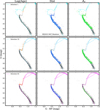 |
Fig. B.1 Selection of different subsets of stars based on their evolutionary phases for the estimation of M67’s log(Age) (orange stars), distance (blue stars) and AV (green stars), at three different iteration steps of the first loop (see Sect. 3.5). |
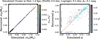 |
Fig. C.1 Same as Fig. 4 but using conditional sampling of the mass-q posteriors while keeping the cluster parameters fixed. |
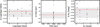 |
Fig. D.1 Recovery of cluster parameters for 24 simulated clusters of solar metallicity placed at 1 kpc. The region between the 16th and the 84th percentiles is enclosed by the gray shaded area. |
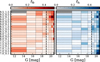 |
Fig. D.2 Left : Fraction of falsely predicted binaries defined in Eq. D.1 in each G mag bin for 24 simulated solar metallicity clusters placed at 1 kpc. The clusters are labelled as "log(Age)_AV". Right : Similar to left but for fraction of falsely predicted singles. Gray coloured bins indicate zero predicted or true binaries. The bold vertical dashed line indicates G = 19 mag. |
Appendix E Additional figures
In Fig. E.1, we study the signature of mass segregation in NGC 2360 and NGC 2682 and how the inclusion of masses of binary companions affects our conclusion about the mass segregation effect in OCs. We adopt the methodology described by Allison et al. (2009), constructing a Minimum Spanning Tree (MST; e.g. Kruskal 1956; Prim 1957) to quantify the degree of mass segregation. Comparing the length of the MST of the most massive stars in a cluster to the one corresponding to a random spatial distribution, we can compute their ratio as ΛMSR for different numbers of stars used to construct the tree, NMST. We refer the reader to Allison et al. (2009) for further details about the method. In Fig. E.1, we use the total mass of the binary system, MA(1 + q), and only the primary mass, MA, to construct the MST in the left and right panels of the figure, respectively. We find that accounting for the companion mass significantly alters the inferred degree of mass segregation, particularly in the case of M67. While considering the total mass of unresolved binaries, the cluster is observed to be mass segregated up to approximately the 350 most massive systems. In contrast, using only the primary mass results in the conclusion of a weak mass segregation signature in M67 among only the ∼20 most massive stars.
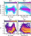 |
Fig. D.3 Dependence of the q residuals (top) and predicted uncertainties (bottom) on the absolute G magnitude (left) and simulated q (right). The solid and dashed lines denote the median and 16th-84th percentile ranges, respectively. The shaded region indicates qpred > 1, values that are unphysical for a binary and therefore not permitted within our framework. |
Appendix F Published tables
Inferred cluster parameters (extract).
Preview of the final table containing cluster members’ source IDs, posterior type used, weighted mode of MA and q, used in estimating which cluster parameters, probability of being single, number of valid samples, and mass ratio threshold applied.
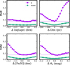 |
Fig. D.4 Mean Absolute Error (MAE) in stellar masses and mass ratios for varying offsets in the mean cluster priors from the true values in case of a solar metallicity cluster simulated at 1 kpc with age 3.5 Gyr and 0.1 AV. The dashed line indicates the MAE in q estimates for an ideal scenario of perfect inference of cluster parameters. |
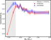 |
Fig. D.5 Reliability of the recovered variation of binary fraction w.r.t MA. We do this test to verify that the observed agreement in Fig. 9 is not dominated by our mass-ratio prior for masses ≳0.6 M⊙. |
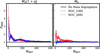 |
Fig. E.1 Effect of mass-segregation shown by mass-segregation ratio (ΛMSR) as a function of the number of stars used to construct the MST (NMST). Left : The total mass of the binary system is considered while constructing the MST. Right : Only the primary mass is used. The solid black line indicates the case of no mass segregation. |
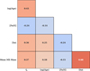 |
Fig. E.2 Kendall correlation matrix for the estimated fb (q ≥ 0.6), the cluster parameters viz., log(Age), distance and [Fe/H] along with the mean mass of the MS stars. Also see Fig. 8. |
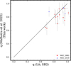 |
Fig. E.3 Comparison of the recovered mass ratios with the corresponding estimates for double-lined spectroscopic binaries (SB2) in M67 (red circles) and NGC 2516 (blue triangles) provided by Geller et al. (2021) and Lipartito et al. (2021) respectively. |
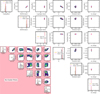 |
Fig. E.4 Complete version of Fig. 2 where the unweighted posteriors corresponding to the case of not using the cluster parameter information are shown in the lower shaded plot. The weighted modes estimated for each astrophysical parameter are indicated by the pink dotted lines. |
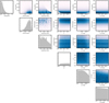 |
Fig. E.5 Distribution of model parameters of 2 million simulated single stars and unresolved binary systems. |
All Tables
Prior distributions for the model parameters we used to generate the simulated training dataset.
Preview of the final table containing cluster members’ source IDs, posterior type used, weighted mode of MA and q, used in estimating which cluster parameters, probability of being single, number of valid samples, and mass ratio threshold applied.
All Figures
|
Fig. 1 Schematic diagram showing the workflow with which we obtained the joint-posterior distribution of the stellar mass and mass ratio while iteratively updating the cluster parameters until convergence. |
| In the text | |
|
Fig. 2 Corner plots of SBI posteriors for a simulated low-mass binary star (MA ~ 0.76 M⊙, q ~ 0.85, d = 1 kpc, AV ~ 0.48 mag, log(Age) [dex] = 9.5, and [Fe/H] [dex] = 0.0) with typical Gaia DR3 and 2MASS/WISE uncertainties for two cases: without (red) and with (blue) prior information about the cluster parameters to obtain the weighted posterior distribution. |
| In the text | |
|
Fig. 3 Convergence of the iterative fitting loop (see Fig. 1) for M67 (NGC 2682). Left panel: PARSEC isochrone fits to the observed CMD for each iteration. Right panels: variation in the cluster parameters in the iterations before they converged in the first round at the 45th iteration. |
| In the text | |
|
Fig. 4 Recovered masses and mass ratios of stars in a simulated solar metallicity cluster (d = 1 kpc, AV ~ 0.1 mag, and log(Age) = 9.5 dex). The modes of the unweighted (top) and weighted (bottom), using cluster parameter information, MA and q posteriors are shown with respect to the simulated parameters. The colour of each data point represents the (fractional) uncertainty in the corresponding (MA) q, and the black data points correspond to stars that are not on the MS or have G ≥ 19 mag. The dashed line in the bottom right panel indicates the qthresh (see text for details) above which we can reliably predict the mass ratio of an unresolved binary in this cluster. |
| In the text | |
|
Fig. 5 Colour-magnitude diagrams of NGC 2360 (top) and NGC 2682 (M67; bottom). For each cluster, the CMDs are coloured by the primary masses and mass ratios (left) and the corresponding uncertainties (right). The identified photometric outliers are shown by red crosses, and the grey shaded region encloses the MS stars with G ≤ 19 mag. The inferred cluster parameters, along with the spectroscopic metallicity, are listed at the top of each panel. |
| In the text | |
|
Fig. 6 Variation in the unresolved binary fraction with the primary mass (left) and with the radial distance (adopted from HR24) from the cluster centre in units of rc (right). The grey shaded region enclosed by the dashed vertical lines indicates the mass range in common between the two clusters. |
| In the text | |
|
Fig. 7 q distributions of the detected unresolved binaries (in the mass range of 0.49-1.2 M⊙) in NGC 2360 and NGC 2682 (M67) shown by red and blue lines, respectively. The grey shaded region indicates the mass-ratio bins below qthresh;Gaia, and the estimated binary fractions for the two mass-ratio thresholds, i.e. qthresh;Gaia and qthresh;Gaia+, are reported along with the Poisson uncertainties. |
| In the text | |
|
Fig. 8 Dependence of the unresolved binary fraction with a high mass ratio (q ≥ 0.6), fb, with the cluster-wide parameters, i.e. log(Age) (left), distance (middle), and [Fe/H] (right) for the 42 OCs. The data points are coloured by the mean mass of MS primary stars. The grey error bars represent the Poisson uncertainties in the binary fractions and 1σ errors in the cluster parameters. |
| In the text | |
|
Fig. 9 Variation in the unresolved binary fraction with the mass of the primary star for all detected binaries (red) and for high mass-ratio binaries alone (q ≥ 0.6; blue). The fit provided by Arenou (2011), our Eq. (1), to the observed variation in the field is overplotted by the dashed black line. The shaded region corresponds to the masses ≤0.6M⊙, wherein the binary fractions are expected to be spuriously inflated due to colour deviations of the observed Gaia DR3 photometry from the PARSEC isochrones. |
| In the text | |
|
Fig. 10 Comparison of the total mass of unresolved binaries with the stellar masses of the cluster members provided in the literature. (a) HR24; (b) Khalatyan et al. (2024); (c and d) Individual and total stellar masses i.e. including the masses of companions provided by AMD23. The red (solid), orange (dash-dotted) and the blue (dashed) lines indicate the q = 0, q = 0.5 and q = 1 relations, respectively. The dashed black line in panel (d) is the one-to-one line, and the pink circles in panel (c) are the inconsistent AMD23 stellar masses reported for BH 99 members (see text for details). |
| In the text | |
|
Fig. 11 Comparison of the predicted mass ratios with estimates by AMD23 (left) and Childs25 (right). The shaded region indicates the low-q region, and the solid and dashed red lines denote the running median and the 16th to 84th percentiles, respectively. |
| In the text | |
|
Fig. 12 Comparison of high mass-ratio (q > 0.6) binary fractions with the literature while using the same mass range, when available. |
| In the text | |
|
Fig. 13 Comparison of the cluster parameters with the literature. The coloured data points denote the estimates from Bossini et al. 2019; Cantat-Gaudin et al. 2020; Dias et al. 2021, and the grey circles indicate the parameters inferred by Hunt & Reffert 2023 and Cavallo et al. 2024. The dashed red line indicates the line of ideal agreement. |
| In the text | |
|
Fig. A.1 G mag distribution of HR24 member stars of 42 OCs divided into different sets based on the availability of good photometry (see text for more details) from 2MASS and WISE. The dashed vertical line marks G = 19 mag, beyond which very few stars have good photometric measurements. |
| In the text | |
|
Fig. B.1 Selection of different subsets of stars based on their evolutionary phases for the estimation of M67’s log(Age) (orange stars), distance (blue stars) and AV (green stars), at three different iteration steps of the first loop (see Sect. 3.5). |
| In the text | |
|
Fig. C.1 Same as Fig. 4 but using conditional sampling of the mass-q posteriors while keeping the cluster parameters fixed. |
| In the text | |
|
Fig. D.1 Recovery of cluster parameters for 24 simulated clusters of solar metallicity placed at 1 kpc. The region between the 16th and the 84th percentiles is enclosed by the gray shaded area. |
| In the text | |
|
Fig. D.2 Left : Fraction of falsely predicted binaries defined in Eq. D.1 in each G mag bin for 24 simulated solar metallicity clusters placed at 1 kpc. The clusters are labelled as "log(Age)_AV". Right : Similar to left but for fraction of falsely predicted singles. Gray coloured bins indicate zero predicted or true binaries. The bold vertical dashed line indicates G = 19 mag. |
| In the text | |
|
Fig. D.3 Dependence of the q residuals (top) and predicted uncertainties (bottom) on the absolute G magnitude (left) and simulated q (right). The solid and dashed lines denote the median and 16th-84th percentile ranges, respectively. The shaded region indicates qpred > 1, values that are unphysical for a binary and therefore not permitted within our framework. |
| In the text | |
|
Fig. D.4 Mean Absolute Error (MAE) in stellar masses and mass ratios for varying offsets in the mean cluster priors from the true values in case of a solar metallicity cluster simulated at 1 kpc with age 3.5 Gyr and 0.1 AV. The dashed line indicates the MAE in q estimates for an ideal scenario of perfect inference of cluster parameters. |
| In the text | |
|
Fig. D.5 Reliability of the recovered variation of binary fraction w.r.t MA. We do this test to verify that the observed agreement in Fig. 9 is not dominated by our mass-ratio prior for masses ≳0.6 M⊙. |
| In the text | |
|
Fig. E.1 Effect of mass-segregation shown by mass-segregation ratio (ΛMSR) as a function of the number of stars used to construct the MST (NMST). Left : The total mass of the binary system is considered while constructing the MST. Right : Only the primary mass is used. The solid black line indicates the case of no mass segregation. |
| In the text | |
|
Fig. E.2 Kendall correlation matrix for the estimated fb (q ≥ 0.6), the cluster parameters viz., log(Age), distance and [Fe/H] along with the mean mass of the MS stars. Also see Fig. 8. |
| In the text | |
|
Fig. E.3 Comparison of the recovered mass ratios with the corresponding estimates for double-lined spectroscopic binaries (SB2) in M67 (red circles) and NGC 2516 (blue triangles) provided by Geller et al. (2021) and Lipartito et al. (2021) respectively. |
| In the text | |
|
Fig. E.4 Complete version of Fig. 2 where the unweighted posteriors corresponding to the case of not using the cluster parameter information are shown in the lower shaded plot. The weighted modes estimated for each astrophysical parameter are indicated by the pink dotted lines. |
| In the text | |
|
Fig. E.5 Distribution of model parameters of 2 million simulated single stars and unresolved binary systems. |
| In the text | |
Current usage metrics show cumulative count of Article Views (full-text article views including HTML views, PDF and ePub downloads, according to the available data) and Abstracts Views on Vision4Press platform.
Data correspond to usage on the plateform after 2015. The current usage metrics is available 48-96 hours after online publication and is updated daily on week days.
Initial download of the metrics may take a while.