| Issue |
A&A
Volume 706, February 2026
|
|
|---|---|---|
| Article Number | A14 | |
| Number of page(s) | 12 | |
| Section | Stellar structure and evolution | |
| DOI | https://doi.org/10.1051/0004-6361/202557568 | |
| Published online | 27 January 2026 | |
The evolutionary history of ultra-compact accreting binaries
I. Chemical abundances and the formation channel of the eclipsing AM CVn system ZTF J225237.05−051917.4 from HST spectroscopy
1
Hamburg Observatory, University of Hamburg Gojenbergsweg 112 21029 Hamburg, Germany
2
European Southern Observatory Karl-Schwarzschild-Strasse 2 85748 Garching bei München, Germany
3
Department of Physics and Astronomy, Texas Tech University 2500 Broadway Lubbock TX 79409, USA
4
Department of Physics, University of Warwick Coventry CV4 7AL, UK
5
Institut für Theoretische Physik und Astrophysik, University of Kiel 24098 Kiel, Germany
6
São Paulo State University (UNESP), School of Engineering and Sciences Guaratinguetá, Brazil
7
The Observatories of the Carnegie Institution for Science Pasadena CA 91101, USA
8
Department of Physics, University of California Santa Barbara CA 93106, USA
9
Departamento de Física, Universidad Técnica Federico Santa María Av. España 1680 Valparaíso, Chile
10
Institute of Science and Technology Austria Am Campus 1 3400 Klosterneuburg, Austria
11
Anton Pannekoek Institute for Astronomy, University of Amsterdam 1090 GE Amsterdam, The Netherlands
12
American Association of Variable Star Observers (AAVSO), 185 Alewife Brook Pkwy Suite 410 Cambridge MA 02138, USA
13
Observadores de Supernovas (ObSN), Observatorio Cerro del Viento, MPC I84, Pl. Fernández Pirfano 3-5A Badajoz 06010, Spain
14
Silesian University of Technology Akademicka 16 Gliwice, Poland
15
INAF - Osservatorio Astronomico di Capodimonte Salita Moiariello 16 80131 Naples, Italy
16
Observadores de Supernovas (ObSN), Observatorio Estelia, MPC Y90, C/ Ladines 12 Ladines Asturias 33993, Spain
17
Observadores de Supernovas (ObSN), Observatorio Uraniborg C/ Antequera 8 41400 Écija Sevilla, Spain
18
Homer L. Dodge Department of Physics and Astronomy, University of Oklahoma 440 W. Brooks Street Norman OK 73019, USA
19
JILA, University of Colorado and National Institute of Standards and Technology 440 UCB Boulder CO 80309-0440, USA
20
Department of Astrophysics/IMAPP, Radboud University PO Box 9010 6500 GL Nijmegen, The Netherlands
21
Department of Astronomy, University of Cape Town Private Bag X3 Rondebosch 7701, South Africa
22
South African Astronomical Observatory PO Box 9 Observatory 7935, South Africa
23
Vereniging Voor Sterrenkunde (VVS) Zeeweg 96 8200 Brugge, Belgium
24
Groupe Européen d’Observations Stellaires (GEOS) 23 Parc de Levesville 28300 Bailleau l’Eveque, France
25
Bundesdeutsche Arbeitsgemeinschaft für Veränderliche Sterne (BAV) Munsterdamm 90 12169 Berlin, Germany
26
School of Physics and Astronomy, University of Southampton Highfield Southampton SO17 1BJ, UK
27
Observadores de Supernovas (ObSN), Observatorio Carpe Noctem, MPC I72 Paseo de la Maliciosa 11 Collado Mediano Madrid 28027, Spain
28
Observadores de Supernovas (ObSN), Observatorio de Sencelles, MPC K14 Camí de Sonfred 1 Sencelles Islas Baleares 07140, Spain
29
American Association of Variable Star Observers (AAVSO) 5 Inverness Way Hillsborough CA 94010, USA
30
Observadores de Supernovas (ObSN), Observatorio Montcabrer, MPC 213 C/ Jaume Balmes 24 Cabrils Barcelona 08348, Spain
31
Dipartimento di Fisica, Università di Pisa 56127 Pisa, Italy
32
Armagh Observatory & Planetarium College Hill Armagh BT61 9DG, UK
33
Observadores de Supernovas (ObSN), Observatorio de Masquefa, MPC 232 Av. Can Marcet 41 Masquefa Barcelona 08783, Spain
34
Instituto de Astrofísica de Canarias E-38205 La Laguna Tenerife, Spain
35
Departamento de Astrofísica, Universidad de La Laguna E-38206 La Laguna Tenerife, Spain
36
Observadores de Supernovas (ObSN), Cal Maciarol mòdul 8 Observatory, MPC A02, Masia Cal Maciarol Camí de l’Observatori s/n Áger Lleida 25691, Spain
37
Department of Astrophysics and Planetary Science, Villanova University Villanova PA 19085, USA
38
Department of Astronomy, University of Washington Seattle WA 98195, USA
39
Instituto de Astronomía, Universidad Nacional Autónoma de México Ciudad Universitaria 04510 CDMX, México.
★ Corresponding author: This email address is being protected from spambots. You need JavaScript enabled to view it.
Received:
6
October
2025
Accepted:
29
November
2025
Abstract
Context. AM Canum Venaticorum (AM CVn) stars are ultra-compact binary systems composed of a white dwarf primary accreting from a hydrogen-deficient donor. They play a crucial role in astrophysics as potential progenitors of Type Ia supernovae and as laboratories for gravitational wave studies. However, their formation and evolutionary history remain incomplete. Three formation channels have been discussed in the literature: the white dwarf, He-star, and cataclysmic variable channels.
Aims. The chemical composition of the accretor atmosphere reflects the material transferred from the donor. In this work we took the first accurate measurements of the fundamental parameters of the accreting white dwarf in ZTF J225237.05−051917.4, including the abundances of key elements such as carbon, nitrogen, and silicon, by analysing ultraviolet spectra obtained with the Hubble Space Telescope (HST). These measurements provide new insight into the evolutionary history of the system and, together with existing optical observations, establish it as a benchmark to develop our pipeline, paving the way for its application to a larger sample of AM CVn systems.
Methods. We determined the binary parameters through photometric analysis and constrained the atmospheric parameters of the white dwarf accretor, including its effective temperature, surface gravity, and chemical abundances, by fitting the HST ultraviolet spectrum with synthetic spectral models. We then inferred the system’s formation channel by comparing the results with theoretical evolutionary models.
Results. According to our measurements, the accretor’s effective temperature (Teff) is 23 300 ± 600 K and the surface gravity (log g) is 8.4 ± 0.3, which imply an accretor mass (MWD) of 0.86 ± 0.16 M⊙. We find a high nitrogen-to-carbon abundance ratio by mass of > 153.
Conclusions. The accretor is significantly hotter than previous estimates based on simplified blackbody fits to the spectral energy distribution, underscoring the importance of detailed spectral modelling for accurately determining system parameters. Our results show that ultraviolet spectroscopy is well suited to constraining the formation channels of AM CVn systems. Of the three proposed formation channels, the He-star channel can be excluded given the high nitrogen-to-carbon ratio. Our results are consistent with both the white dwarf and cataclysmic variable channels.
Key words: stars: atmospheres / binaries: eclipsing / binaries: spectroscopic / novae / cataclysmic variables / white dwarfs
© The Authors 2026
 Open Access article, published by EDP Sciences, under the terms of the Creative Commons Attribution License (https://creativecommons.org/licenses/by/4.0), which permits unrestricted use, distribution, and reproduction in any medium, provided the original work is properly cited.
This article is published in open access under the Subscribe to Open model. This email address is being protected from spambots. You need JavaScript enabled to view it. to support open access publication.
1. Introduction
AM Canum Venaticorum (AM CVn) stars are ultra-compact accreting binaries composed of a white dwarf (WD) primary and a hydrogen-deficient donor. Depending on their evolutionary history, donor stars can be WDs or semi-degenerate He stars. These systems are crucial in several areas of astrophysics: (1) they serve as probes of stellar evolution, representing the final stages of close binary evolution; (2) they are potential progenitors of Type Ia supernovae; and (3) they act as laboratories for gravitational wave (GW) astrophysics. The number of known AM CVn systems has increased significantly, from a few dozen in the early 2000s to more than one hundred today, mainly thanks to large surveys (Roelofs et al. 2007; Solheim 2010; Ramsay et al. 2018; Pichardo Marcano et al. 2021; Green et al. 2025). With ongoing and upcoming surveys, including the BlackGEM project (Groot et al. 2024), the Gravitational-wave Optical Transient Observer (GOTO; Steeghs et al. 2022), the Sloan Digital Sky Survey – V (SDSS; Kollmeier et al. 2025), and the Legacy Survey of Space and Time (LSST; Ivezić et al. 2019), many more are expected to be discovered. With the growing sample, it is timely to develop a more detailed understanding of these systems.
An AM CVn system descends from binary main-sequence stars, in which the more massive component evolves first off the main sequence and enters the giant phase. This leads to a binary interaction event, which can proceed through either stable Roche-lobe overflow or a common envelope phase (Brown et al. 2016; Li et al. 2023). This interaction episode leaves behind a more compact binary with a WD primary. Three widely accepted evolutionary channels can follow: (i) In the WD channel, the secondary evolves off the main sequence and the system undergoes a second interaction, leading to a double WD binary. GW radiation then shrinks the orbit to periods as short as five minutes, after which stable mass transfer begins (Paczyński 1967; Webbink 1984; Nelemans et al. 2001; Deloye et al. 2007; Wong & Bildsten 2021; Chen et al. 2022). (ii) The He-star channel also involves a second interaction episode but leaves behind a semi-degenerate, helium-rich donor. In this case, the initially non-degenerate donor, being less compact, causes mass transfer at longer orbital periods, typically around 15 minutes (Savonije et al. 1986; Iben & Tutukov 1987; Yungelson 2008; Bauer & Kupfer 2021). (iii) The cataclysmic variable (CV) channel differs from the other two as this scenario originates in a CV system and involves only one interaction phase. The helium core of the donor is exposed once its outer layers are stripped through stable mass transfer, during which the accreted material transitions from hydrogen-rich to helium-rich (Tutukov et al. 1985; Podsiadlowski et al. 2003; Goliasch & Nelson 2015; Liu et al. 2021; Belloni & Schreiber 2023; Sarkar et al. 2023).
A possible final fate of an AM CVn system is the explosive event of a Type Ia supernova, one of the most important classes of astronomical transients. In the so-called ‘double-detonation’ scenario, a surface helium detonation occurs on a WD after it has accreted sufficient material from a helium-rich donor (Nomoto 1982; Bildsten et al. 2007; Fink et al. 2010; Shen et al. 2018b,a; Wang 2018; Wong & Bildsten 2023; Rajamuthukumar et al. 2025). When this helium layer reaches a critical mass, it ignites and can trigger a secondary detonation in the carbon–oxygen (CO) core of the WD, resulting in a thermonuclear explosion. This scenario is particularly relevant for sub-Chandrasekhar mass WDs, as it does not require the WD to exceed the Chandrasekhar limit. A double-shell morphology of a supernova remnant was recently reported by Das et al. (2025), providing observational evidence of the existence of this explosion mechanism in nature.
Owing to their compact orbits and relatively small distances to Earth, AM CVn systems are among the strongest sources of GWs in the millihertz band, the operating range of the forthcoming Laser Interferometer Space Antenna (LISA) and TianQin missions (Amaro-Seoane et al. 2023; Luo et al. 2016). Many AM CVn binaries will be detectable within weeks to months of the launch of LISA and will serve as verification sources for instrument calibration and early science (Nelemans et al. 2004; Kremer et al. 2017; Kupfer et al. 2018). Kupfer et al. (2024) identified 40 Galactic binaries likely to be detected by LISA, including 18 verification sources1. Among these, 16 AM CVn systems are expected to be detected after 48 months, and 2 may be resolved within just two months. With the anticipated launch of LISA in the 2030s, detailed electromagnetic characterisation of these systems is essential. Such efforts will improve the interpretation of GW sources, enable multi-messenger studies, and enhance the calibration of GW observatories. Systems that are not individually resolved will still contribute to the Galactic confusion foreground, produced by compact binaries in the Milky Way, which can limit sensitivity to weak signals (Breivik et al. 2020; Korol et al. 2022; Littenberg & Lali 2025).
A critical question in the study of AM CVn systems is the relative contribution of their formation channels. This constrains binary population synthesis predictions of their space densities and period distributions. One possible way to distinguish between the channels is through the chemical composition of the donor (Nelemans et al. 2010). While in a few cases there are indications that the donor is detectable in the infrared (Green et al. 2020; Rivera Sandoval et al. 2021), donors are more commonly intrinsically faint and challenging to observe directly. Their composition can therefore be inferred from the surface abundances of the accreting WD, which trace the material stripped from the donor. This indirect approach enables reconstruction of the evolutionary history of the system. In particular, the N/O and N/C ratios vary strongly due to different levels of CNO and He burning. The key diagnostic is the N/C ratio, which differs by more than an order of magnitude, from N/C ≲ 10 for systems with a He-star donor to N/C ≳ 100 for both the WD and CV channels. Models of the CV channel have traditionally struggled to reproduce the observed systems, as they predict a modest amount of residual hydrogen (Schenker et al. 2002; Podsiadlowski et al. 2003). Recent studies, however, suggest that modifications such as enhanced magnetic braking may resolve these difficulties, potentially allowing donors to retain hydrogen at levels below current detection thresholds (Belloni & Schreiber 2023; Sarkar et al. 2023).
High-quality ultraviolet (UV) spectroscopy is essential for stellar atmosphere analysis of compact accreting binaries. Optical observations alone are insufficient, as the accretion disc dominates the system flux and outshines the WD in the optical and (near-)infrared band. Moreover, absorption features of key elements such as silicon, nitrogen, carbon, and oxygen are primarily detectable in the UV. Space-based spectroscopy is therefore the only means of accurately determining the system parameters, such as effective temperature (Teff), surface gravity (log g), and elemental abundances. The only currently operational telescope capable of such observations is the Hubble Space Telescope (HST). In response to this need, a large HST Treasury observing campaign (PI: A. F. Pala) was carried out, targeting 31 accreting WD binaries, including 12 AM CVn systems.
We used one of these 12 as a benchmark target: the eclipsing system ZTF J225237.05−051917.4 (hereafter ZTF J2252−05), which has an orbital period of 37.4 min. This system was discovered by van Roestel et al. (2022), who carried out optical follow-up. Observations from the Zwicky Transient Facility (ZTF; Bellm et al. 2019), together with high-speed photometry with Chimera on the Hale Telescope, enabled precise measurements of the orbital period (Porb) and mass ratio (q). In addition, optical spectroscopy obtained with the Low Resolution Imaging Spectrometer (LRIS) on the Keck I telescope revealed a helium-dominated atmosphere with no detectable hydrogen features. Unlike other AM CVn systems, ZTF J2252−05 has a highly comprehensive observational dataset. It is therefore well suited to serve as a foundation for developing a pipeline to constrain the physical parameters of such systems spectroscopically.
This paper is structured as follows. Section 2 presents the observational data, including ground-based photometry in addition to the HST observations, and describes the structure and processing of the time-resolved UV spectroscopy. Section 3 details the methods used for light curve and spectral modelling. The results of the spectral analysis are given in Sect. 4, and the evolutionary history is discussed in Sect. 5. Section 6 summarises our findings and outlines the steps required to build the first statistically significant spectroscopic sample of AM CVn stars to study their evolution.
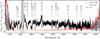 |
Fig. 1. Average HST/COS spectrum of ZTF J2252−05 covering 900–2050 Å. Masked regions include areas of low sensitivity (< 1100 and > 1850 Å; grey) and geocoronal Lyα at 1215 Å (shaded). Night-only data were used to reduce airglow contamination. The error of the averaged flux is shown in red. |
2. Observations
ZTF J2252−05 was observed using the Cosmic Origins Spectrograph (COS) on board HST on 2022 November 17 with a total exposure time of 11 564 s over five spacecraft orbits. The G140L grating was used with a central wavelength of 800 Å, covering 900–2150 Å at R ≃ 3000. It was observed as part of a large HST Treasury programme (Cycle 29; ID: 16659 and 17401; PI: A. F. Pala), which includes 31 accreting WDs, among them 12 AM CVn systems (11 of which have been observed at the time of writing). The observational information of the AM CVn targets is summarised in Table 1. Orbital periods Porb (excluding ZTF J2252−05) are adopted from Green et al. (2025). A comprehensive discussion of the AM CVn sample, together with the broader set of accreting binaries in the programme, will be presented in future work.
AM CVn targets observed in HST programme 16659 and 17401.
2.1. Ultraviolet observations
The COS-averaged UV spectrum of ZTF J2252−05 is shown in Fig. 1. The usable wavelength range extends from 1100 to 1800 Å, where the noise level is sufficiently low (S/N ≳ 4 on the pseudo-continuum). The Geocoronal Lyα contaminated region (1196–1225 Å) is masked. To recover the photospheric O I absorption line at 1304 Å, we used only night-time HST data, when the Sun was below the Earth limb and geocoronal airglow was minimal. The average spectrum is then obtained by patching the clean O I region into the full spectrum, to preserve high S/N elsewhere.
The data were obtained in TIME-TAG mode, which also allows us to extract the light curve, following a method similar to that described in Pala et al. (2022). By plotting photon positions in the cross-dispersion direction (YFULL) against their corresponding wavelengths, we defined a rectangular region centred on the target spectrum. Two parallel background regions, one on each side of the target spectrum, are also selected for calibration. Photon events were binned into 3 s intervals. The source signal was extracted by counting events within the rectangular aperture corresponding to the target, and corrected for background counts measured in adjacent regions to produce the light curve (Fig. 2).
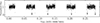 |
Fig. 2. Normalised UV light curve of ZTF J2252−05, extracted from time-resolved COS observations. The total exposure time was 11 563 s, covering five eclipses. The gaps correspond to intervals when the target was behind the Earth and not visible to HST. |
2.2. Brightness monitoring
Due to the intrinsic variability of accreting binary systems, observations of accreting WDs are only safe during quiescence. Observing the target during a disc outburst, when the system brightness increases by a factor of 2–8, could exceed the COS safety thresholds and pose a risk to the detectors. In addition, during an outburst, the disc dominates the emission, which prevents the detection of the WD. Following the procedure described in previous works (Pala et al. 2017; Tovmassian et al. 2025), we therefore conducted a photometric monitoring campaign in the weeks preceding the scheduled HST observations to ensure both safety and scientific return. Photometry was obtained using the robotic ground-based telescopes of the Las Cumbres Observatory (LCO; Brown et al. 2013), complemented by coordinated observations from citizen scientists affiliated with the American Association of Variable Star Observers (AAVSO) and the Observadores de Supernovas (ObSN) group. Figure 3 shows the brightness of ZTF J2252−05 in the weeks around the HST visit, remaining stable at V ≈ 19 mag and indicating that the system was in quiescence.
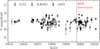 |
Fig. 3. Photometric monitoring of ZTF J2252−05, including observations from LCO, AAVSO, and ObSN. The vertical dashed line highlights the time of the HST observations (2022 November 17). Fluctuations can occur during monitoring, as a single exposure may coincide with, or partially cover, an eclipse (≃1.5 min) of the WD. |
3. Methods
3.1. Light curve analysis
The light curve analysis of ZTF J2252−05 provides a baseline for understanding the system and serves as a reference for the subsequent spectral analysis by constraining the binary parameters. Geocoronal Lyα and O I, together with strong disc emission features (N V and Si IV) that do not originate from the WD, were masked. We modelled the eclipsing UV light curve with the LCURVE software package (Copperwheat et al. 2010). The best-fitting model is shown in Fig. 4, and the key corresponding parameters are listed in Table 3. We adopted the binary parameters, such as Porb and q, from van Roestel et al. (2022), who derived them from high-time-resolution optical photometry. The donor radius, Rdonor, was determined from q under the assumption of Roche-lobe filling (Eggleton 1983). We modelled the individual components of the system, namely the WD, the accretion disc, and the bright spot (the region where the accreting material impacts the outer edge of the disc), following the approach of Green et al. (2018). The free parameters of the model are the inclination, WD radius, component temperatures (WD, donor, disc, and bright spot), and the reference epoch T0, defined as the mid-eclipse time.
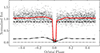 |
Fig. 4. Fitted UV light curve of ZTF J2252−05. The black points show the light curve binned into 3 s intervals. The best-fit model (red) includes contributions from the accreting WD (dashed line), the bright spot (dash-dotted line), and the accretion disc (dotted line). The residuals are shown below the light curve. |
This allows us to estimate the relative contributions of the components to the total flux. The model indicates that the accreting WD contributes 84% of the UV flux, the bright spot 16%, and the disc less than 0.1%. The disc contribution is therefore negligible and excluded from the subsequent spectral analysis. In the optical, the bright spot becomes increasingly relevant towards shorter wavelengths, contributing 3%, 5%, and 7% in the i, r, and g bands, respectively (van Roestel et al. 2022). This trend reflects its high temperature (> 14 000 K), in contrast to the cooler disc (∼5000 K), which dominates the optical flux but has no significant impact in the UV.
3.2. Spectral analysis
3.2.1. Interstellar medium contamination
Extinction and absorption features from the interstellar medium (ISM) must be accounted for in the analysis of stellar atmospheres. ZTF J2252−05 is located at Galactic coordinates (l, b) = (76.96° , − 46.67° ) with a distance of  pc. The distance was reported by van Roestel et al. (2022), based on the Gaia DR3 parallax (Gaia Collaboration & Brown 2021) and a prior constructed from the Galactic WD distribution (Kupfer et al. 2018). The extinction is AV = 0.149 ± 0.007 from the 3D Galactic dust maps (G-Tomo; Lallement et al. 2022; Vergely et al. 2022), which for RV = 3.1 returns E(B − V) = 0.048 ± 0.002. We then reddened our model accordingly following the wavelength-dependent extinction law from Cardelli et al. (1989).
To assess possible contamination by interstellar metal lines, we compared the spectrum of ZTF J2252−05 with that of a target, WD 2253−062 (RA: 22:55:47.52, Dec: −06 : 00 : 50.67; (l, b) = (65.21° , − 55.34° ); d = 67.8 pc). Located only 63′ away from ZTF J2252−05, it is the closest WD on the sky with a pristine hydrogen atmosphere and archival HST observations. It was observed with COS/G130M for an exposure of 2000 s (Cycle 25, ID: 15073; PI: B. Gänsicke). As shown in Fig. 5, the spectra of ZTF J2252−05 and WD 2253−062 both exhibit absorption lines from oxygen and carbon. The prominent C II 1335 Å and O I 1304 Å lines, which are also present in WD 2253−062, indicate an interstellar origin. Therefore, these lines were excluded from the following spectral analysis.
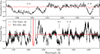 |
Fig. 5. Spectral comparison of ZTF J2252−05 (black) and WD 2253−062 (red). Bottom: Spectrum of WD 2253−062 obtained with the G130M grating, degraded to match the resolution of the ZTF J2252−05 observation with the G140L grating. Top: Zoomed-in view of the potential ISM-contaminated regions around O I 1304 and C II 1335 Å. Both spectra were continuum-normalised. |
Metal absorption lines used in the spectral fitting.
Given the importance of carbon and oxygen as tracers of nuclear burning, we examined the alternative ionisation stages. For oxygen, reliable diagnostic lines are not available within the observed wavelength: the O Iλ1026 Å line lies in the noisy far-UV region, and the broad geocoronal Lyα emission saturates the potential ionised λ1217 Å oxygen feature. As a result, we cannot place a meaningful constraint on the oxygen abundance. For carbon, we can estimate an upper limit of its abundance from the theoretical C I feature near 1280 Å (Sect. 3.3). However, even though ZTF J2252−05 is angularly close to WD 2253−062, it is eight times farther away. Additional ISM contamination cannot be ruled out, and the constraints on carbon from C I are consequently only upper limits.
3.2.2. Spectral fitting
We employed the hydrogen-deficient stellar atmosphere models described by Koester (2010). This framework enables us to vary the abundance of individual elements, denoted Xi, which we defined as the base-10 logarithmic number ratio relative to helium, that is, Xi = log(Ni/NHe), where N denotes the particle number. The chemical profile, denoted {Xi}, therefore represents the atmospheric abundances of all identified elements. Based on the absence of hydrogen lines in the optical spectra (van Roestel et al. 2022) and the lack of an identifiable Lyα broad absorption feature in the UV (Fig. 1), we adopted a conservative lower limit for the hydrogen abundance of XH = −9. By generating grids with different Teff, log g, and {Xi}, we constrained the overall atmospheric properties. The model spectra provide the Eddington flux at the stellar surface, Hλ. To compare the model with the observed flux, Fobs, λ, we applied the scaling
 (1)
(1)
where R is the WD radius and d is the distance to the system. The radius was computed using the mass–radius relation of the Montréal WD cooling models2, based on the evolutionary models of Bédard et al. (2020). A 16% bright-spot flux contribution was estimated from the light curve fit (Sect. 3.1). As no model for the bright-spot emission is available, this contribution was included in the spectral modelling as a secondary flat continuum component in Fλ. We also included the radial velocity vrad as a free parameter to account for wavelength shifts from the WD reflex motion, averaged over the HST exposure time. We describe below the procedure used to measure the atmospheric parameters of the accreting WD in ZTF J2252−05 by fitting its averaged UV spectrum. All spectral fits were carried out using the Markov chain Monte Carlo method, implemented via the emcee Python package (Foreman-Mackey et al. 2013; Hogg & Foreman-Mackey 2018). An overview of the methodology is also presented in the flowchart shown in Fig. 6.
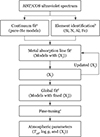 |
Fig. 6. Flowchart of the spectral fitting procedure. Superscripts in the step titles correspond to the steps described in Sect. 3.2.2. |
(a) Continuum fit. We performed the initial fit on the spectrum’s continuum using a grid of pure-helium (DB-type) WD atmosphere models, with Teff from 10 000 to 30 000 K in steps of 500 K, and log g from 7.5 to 9.5 dex in steps of 0.2 dex. Extinction was treated following the approach described in Sect. 3.2.1. This step provided a zeroth-degree estimate of Teff, which was then used as the starting point for the forthcoming spectral fits.
(b) Element identification. As shown in Fig. 1, the elements with absorption lines suitable for reliable fitting are Si, N, Al, and Fe. The absence of a prominent carbon feature suggests a low abundance. An attempt to constrain its upper limit is presented in Sect. 3.3 and is not included in the fitting process.
(c) Individual abundance estimation. Due to computational limitations, we did not vary Teff, log g, and abundances simultaneously. At the early stages, log g was fixed to the value derived from the continuum fit, and model grids were used to explore combinations of Teff and abundances. For example, Si lines were fitted using grids with varying Teff and XSi while holding log g constant. In each iteration, the updated {Xi} from the previous step served as the background, gradually narrowing the parameter space. To minimise blending effects, we restricted the fits for each element to wavelength regions with relatively isolated absorption lines. The fitted lines are listed in Table 2. This iterative procedure forms the basis for determining the complete chemical profile of ZTF J2252−05.
(d) Global fit. Using the chemical profile estimated from the previous step, we constrained Teff and log g by fitting the full spectrum with grids of models at fixed metal abundances. We masked regions affected by geocoronal Lyα contamination and by potential accretion disc emission features (N V and Si IV). The λ1175 Å, λ1549 Å, and λ1640 Å lines, which likely originated from the disc or from veiling gas, were not included in the fit3.
(e) Fine-tuning. Due to line blending, neighbouring absorption lines can influence one another, causing the atmospheric parameters estimated from the global fit (i.e. Teff and log g) to differ slightly from those obtained through initial individual abundance estimations. To resolve this inconsistency, we repeated the individual abundance fitting using the globally determined Teff and log g. The resulting updated chemical profile was then incorporated into a new global fit. This process was iterated until all parameters converge, completing the fitting procedure.
3.2.3. Uncertainty estimation
During the spectral fitting process, the distance and extinction were fixed, and their associated systematic uncertainties were not initially considered. Interstellar extinction affects the slope of the spectral continuum, thereby influencing the measurement of Teff. As shown in Eq. (1), the distance influences the overall flux level quadratically, which in turn affects the measurement of log g. To estimate the systematic uncertainties on the atmospheric parameters, we followed a Monte Carlo approach to independently assess the influence of varying Teff and log g. For extinction, we drew random values from a Gaussian distribution defined by the measured AV and its uncertainty to perform spectral fitting using χ2 minimisation over 5000 iterations. The resulting posterior distributions reflect the systematic uncertainty due to extinction. A similar procedure is repeated for the uncertainty in the distance. These systematic uncertainties are then combined in quadrature with the statistical uncertainties obtained from the Markov chain Monte Carlo analysis. The final atmospheric parameters and uncertainties are listed in Table 3.
System parameters of ZTF J2252−05.
3.3. Carbon and hydrogen abundance constrain
As discussed in Sect. 3.2.1, the C II 1335 Å line is affected by interstellar absorption. No other carbon feature in the observed spectrum is strong enough for a reliable abundance fit, suggesting a carbon-poor atmosphere. However, given the critical role of carbon in nuclear burning and as a tracer of evolutionary channels (Nelemans et al. 2010; Toloza et al. 2023), we attempted to place an upper limit on its abundance using the relatively uncontaminated spectral region near the theoretical C I line at 1280 Å. We simulated a grid of models based on the best-fit spectrum with varying carbon abundances. These were then compared with the observed spectrum of ZTF J2252−05 to determine an upper limit on the carbon abundance. Hydrogen is also a key diagnostic for identifying systems that evolved through the CV channel (Podsiadlowski et al. 2003; Belloni & Schreiber 2023). To test for its presence, we carried out a similar exercise for hydrogen by increasing its abundance stepwise from a conservative lower limit.
4. Results
Figure 7 shows the individual atmospheric models fitted for the identified elements (Si, N, Al, and Fe). These abundances are included in the global fit over the studied wavelength range, and the resulting best-fit stellar atmosphere model is shown in Fig. 8. The parameters derived from the spectral fits are listed in Table 3.
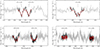 |
Fig. 7. Spectral fits for the individual elements Si, N, Fe, and Al (clockwise from the top left). This corresponds to step (c) described in Sect. 3.2.2. The identified absorption lines (black) are compared with the best-fitting models (red); spectral regions not included in the fit are shown in grey. |
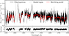 |
Fig. 8. Best-fitting atmospheric model for ZTF J2252−05, computed with the hydrogen-deficient code of Koester (2010) and using the parameters listed in Table 3. The bright spot contribution is included as an additional constant term in Fλ; it accounts for about 16% of the total flux. The model includes Si, N, Al, and Fe. Geocoronal lines, ISM-contaminated regions, potential disc emission, and possible veiling absorption are masked. The residuals are shown below the spectrum. |
The synthetic spectra with varying carbon abundances, based on the best-fit model, are shown in Fig. 9 (left panel). The colour bar indicates the carbon abundance, ranging from XC = −3.0 to XC = −8.0 in steps of 0.5. By comparing the models with the expected C I absorption feature near 1280 Å, we derived an upper limit of XC < −5.00.
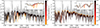 |
Fig. 9. Synthetic spectra with varying carbon (left) and hydrogen (right) abundances overplotted on the observed spectrum (grey). Inset panels highlight the diagnostic regions. Left: Carbon abundances ranging from −8.0 to −3.0. The absence of C I lines near 1280 Å indicates XC < −5.0. Right: Hydrogen abundances from −9.5 to −3.0. Lyα is outshone by geocoronal emission, and no clear hydrogen diagnostic lines are present, leaving the hydrogen abundance unconstrained. |
We fixed a conservative hydrogen abundance of XH = −9 in the global spectral fit, as no hydrogen features were detected in the optical spectroscopic analysis of ZTF J2252−05 (van Roestel et al. 2022). In the UV, the Lyα line at 1215 Å is the most prominent feature but is completely outshone by geocoronal emission. Figure 9 (right panel) shows models with hydrogen abundances ranging from XH = −9.5 to XH = −3.0 in steps of 0.5. Variations in XH primarily affect the continuum, leading to degeneracies with surface gravity. No isolated hydrogen absorption line was available for a reliable estimate of XH, and the hydrogen abundance therefore remains unconstrained.
For the primary WD, the spectral fit yields an effective temperature of Teff = 23 300 ± 600 K and a surface gravity of log g = 8.4 ± 0.3. Using the mass–radius relation from Bédard et al. (2020), we derive a mass of MWD = 0.86 ± 0.16 M⊙ and a radius of RWD = 0.0095 ± 0.0018 R⊙. For the donor star, we adopted a mass ratio of q = 0.034 ± 0.006 from the photometric analysis of van Roestel et al. (2022), which implies a donor radius of Rdonor = 0.049 ± 0.004 R⊙ under the assumption of a Roche-lobe-filling configuration. This yields a donor mass of Mdonor = 0.029 ± 0.008 M⊙, from which we calculated an orbital separation of a = 0.36 ± 0.02 R⊙.
5. Discussion
5.1. Formation channel identification
5.1.1. Chemical abundances
In Sect. 1 we outlined the three main evolutionary channels for AM CVn systems: the WD, the semi-degenerate He-star, and the CV channel. Nelemans et al. (2010) proposed a method for inferring the likely formation pathway based on the observed chemical abundances in the accreting WD’s atmosphere originating from its donor. Their approach combines stellar evolution models (Eggleton & Kiseleva-Eggleton 2002) with magnetic braking prescriptions (Rappaport et al. 1983; Podsiadlowski et al. 2002), showing that the chemical signature of the accreted material traces the evolutionary state of the donor star.
The detection of hydrogen in the spectrum was long regarded as strong evidence for the CV channel (e.g. Podsiadlowski et al. 2003; Solheim 2010), but Belloni & Schreiber (2023) show that this channel can also produce AM CVn systems with undetectable hydrogen abundances (XH ≲ −6). Abundances of elements heavier than helium are likely to be similar between the WD and CV channels (Nelemans et al. 2010). However, distinguishing the He-star channel from other channels is still possible with a detailed assessment of the atmospheric metal abundances. In particular, when material is processed through the CNO cycle, the ratios of carbon, nitrogen, and oxygen evolve in characteristic patterns. Helium burning leads first to the production of carbon, followed by oxygen, effectively enhancing their abundances relative to that of nitrogen. This makes the nitrogen-to-carbon abundance ratio N/C a useful diagnostic: systems formed via the WD or CV channel tend to show a high N/C, while those from the He-star channel show lower values due to ongoing helium burning. Figure 10 illustrates this diagnostic using model predictions of the N/C evolution for various binary configurations.
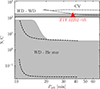 |
Fig. 10. Derived limit N/C > 153 (red triangle) compared with evolutionary models. WD and He-star channel models are taken from Nelemans et al. (2010). WD donor tracks with progenitor masses of 1.0, 1.5, and 2.0 M⊙ (from top to bottom) are shown as solid lines. The possible He-star donor region is indicated by the shaded area, with two examples for initial orbital periods of 20 and 60 min (upper and lower dashed lines). The CV-channel model (dashed line) is calculated using the system parameters listed in Table 3. |
From our spectrum, we estimate log(N/He) = − 2.58 and log(C/He) < − 5.00 (by particle number). Converting these results to a mass ratio using the atomic masses of nitrogen and carbon (mN = 14.007 u and mC = 12.011 u; 1 u = 1.6605 × 10⁻²⁴ g), we obtain a lower limit of N/C > 153. This value is compared with theoretical predictions in Fig. 10; we see that ZTF J2252−05 is well above the range spanned by the He-star models and strongly supporting a WD or CV formation scenario.
5.1.2. Stellar evolutionary models
We compared our estimated parameters with theoretical AM CVn evolutionary models computed using the stellar evolution software Modules for Experiments in Stellar Astrophysics (MESA; Paxton et al. 2011, 2013, 2015, 2018, 2019). In Fig. 11 we present the evolution of Rdonor and Mdonor for the three proposed AM CVn formation channels.
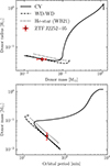 |
Fig. 11. Comparison of the measured donor properties and the theoretical evolutionary tracks computed with MESA. Top: Donor radius (Rdonor) as a function of donor mass (Mdonor). Bottom: Corresponding relation between Mdonor and the orbital period. The CV channel (solid line) and the adiabatic WD channel (dashed line) reproduce the spectroscopically derived parameters. An example He-star channel track (dotted line) from Wong & Bildsten (2021), labelled ‘WD21’, is included for reference. |
The model for the CV channel was computed following Belloni & Schreiber (2023). We ran a grid of models varying the initial Mdonor and the initial Porb, assuming an initial MWD of 0.86 M⊙. Depending on the mass transfer rate, the WD mass can increase, and we adopted the mass growth criteria from Wolf et al. (2013). The value of Mdonor is varied between 1.0 and 1.5 M⊙ in steps of 0.1 M⊙, and the value of Porb between 0.2 and 2.0 days in steps of 0.2 days. The grid is then refined around the region where models reproduce the properties derived from the observational data.
The adiabatic WD channel models were produced following Wong & Bildsten (2021). For each value of central specific entropies Sc, we rapidly reduced the mass of a 0.15 M⊙ He WD (taken from Wong & Bildsten 2023) via a high mass-loss rate to ensure adiabatic evolution, and measured its radius at various points. In this channel, the evolution is governed directly by the donor’s Sc, which sets the mass–radius relation (Deloye et al. 2007), whereas in the CV channel the donor entropy is fixed by the helium core mass at the onset of mass transfer (Belloni & Schreiber 2023). From the adiabatic mass–radius relation, we numerically integrated the orbital evolution equations assuming fully conservative mass transfer and angular momentum loss driven solely by GW radiation (e.g. Bauer & Kupfer 2021). The resulting mass transfer rate is then applied to a CO WD accretor with an initial mass between 0.65 and 0.85 M⊙ to model its accretion-induced reheating and subsequent cooling. The evolution of Teff with Porb is shown in Fig. 12.
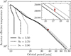 |
Fig. 12. Comparison of the estimated WD effective temperature (Teff) and theoretical WD channel models with varying central entropy (SC). |
The CV and WD–WD evolutionary models reproduce our spectroscopically derived parameters within their uncertainties, indicating consistency between theoretical predictions and observations. Although it is unlikely that this system formed through the He-star channel, for completeness, we present the corresponding donor parameters using models from Wong & Bildsten (2021). This model assumes an adiabatic evolution after the mass of the He-star donor decreases to 0.2 M⊙. As the donor masses of all three tracks overlap considerably within the typical AM CVn Porb range of 5–70 min, identifying the formation channel based on this criterion alone remains challenging. However, this method becomes more promising for systems with shorter Porb, such as ES Cet, KIC 4547333, and HP Lib (see Table 1). Therefore, chemical analysis remains a crucial tool for constraining the formation pathway.
5.2. Comparison with optical results
The mass and radius derived from our spectral fit of the primary WD are consistent with the values reported by van Roestel et al. (2022), who obtained MWD = 0.76 ± 0.05 M⊙ and RWD = 0.010 ± 0.001 R⊙. In contrast, the effective temperature inferred from our fit is significantly higher than their reported value of Teff = 15 200 ± 900 K. A similar exercise by Macrie et al. (2024) yielded Teff = 15 560 ± 460 K. This discrepancy likely reflects differences in the modelling. The earlier studies employed a simplified blackbody fit and adopted a lower extinction value of E(B − V) = 0.01 from Green et al. (2019). This interstellar dust map does not account for sources within 400 pc and likely underestimates the total extinction. Whereas our ISM model, based on the more recent 3D dust map from Lallement et al. (2022), yields E(B − V) = 0.048 and enables a more accurate spectral modelling.
6. Summary and conclusion
We analysed HST/COS time-tagged UV spectroscopy of the AM CVn system ZTF J2252−05. This system was selected as a benchmark target to demonstrate the feasibility of reconstructing the evolutionary history of AM CVn systems through detailed atmospheric spectral fit. By combining updated astrometry from Gaia DR3 (Gaia Collaboration & Brown 2021), extinction corrections from 3D dust maps (Lallement et al. 2022), and published photometry and light curve modelling (van Roestel et al. 2022), we constrained the parameters of the accreting WD using hydrogen-deficient atmospheric models with realistic chemical compositions, applied in this context for the first time.
For the accretor, we determined an effective temperature of 23 300 ± 600 K, a surface gravity of 8.4 ± 0.3, a mass of 0.86 ± 0.16 M⊙, and a radius of 0.0095 ± 0.0018 R⊙. These results highlight the importance of UV spectroscopy for characterising ultra-compact binaries. The derived mass is consistent with that from van Roestel et al. (2022) and supports the view that accretors in AM CVn binaries are generally more massive than typical single WDs (≈0.6 M⊙), more in line with the masses of accretors in CVs (Zorotovic et al. 2011; Pala et al. 2022). The measured Teff is higher than that reported by van Roestel et al. (2022), partly because the extinction was underestimated with the data then available, and further indicates that spectral energy distribution fits with simplified blackbody models may misjudge the accretor temperature, highlighting the need for detailed atmospheric modelling.
We identified absorption features of the accreting WD from Si, N, Al, and Fe, and measured their atmospheric abundances. We also placed an upper limit on the abundance of C, which plays a key role in thermonuclear processes and serves as a tracer of the formation channel. From the measured abundances, we estimated a nitrogen-to-carbon mass ratio (N/C) of > 153. Regarding the three proposed AM CVn formation channels, our results strongly disfavour the He-star channel, while the WD and CV channels remain viable. The presence of hydrogen below the detection limit cannot be excluded, leaving these two channels indistinguishable.
We have developed and validated a robust pipeline for spectral modelling of mass-transferring, hydrogen-deficient ultra-compact binaries. Our results show that atmospheric abundance analysis provides meaningful constraints on the evolutionary origins of individual systems. With this methodology now tested and validated on ZTF J2252−05, we are well positioned to apply the same approach to a larger sample of AM CVn systems. This paves the way towards constructing the first statistically significant spectroscopic population with well-characterised formation channels, placing AM CVn stars within the broader landscape of accreting compact binaries.
Acknowledgments
We thank Lars Bildsten for valuable insights and discussions. We acknowledge with thanks the variable star observations from the AAVSO International Database contributed by observers worldwide and used in this research. We thank the members of the Spanish Observers of Supernovae (ObSN) group for their valuable photometric contributions. This research was supported by Deutsche Forschungsgemeinschaft (DFG, German Research Foundation) under Germany’s Excellence Strategy – EXC 2121 “Quantum Universe” – 390833306. Co-funded by the European Union (ERC, CompactBINARIES, 101078773). Views and opinions expressed are however those of the author(s) only and do not necessarily reflect those of the European Union or the European Research Council. Neither the European Union nor the granting authority can be held responsible for them. DB acknowledges support from the São Paulo Research Foundation (FAPESP), Brazil, Process Numbers #2024/03736-2 and #2025/00817-4. MRS is supported by Fondecyt (grant 1221059). MJG acknowledges support from the European Research Council through ERC Advanced Grant No. 101054731, from the National Aeronautics and Space Administration under grants 80NSSC24K0436, 80NSSC22K0479, and 80NSSC24K0380, and from the National Science Foundation under grant AST-2205736. PJG is supported by NRF SARChI grant 111692. PR-G acknowledges support by the Agencia Estatal de Investigación del Ministerio de Ciencia e Innovación (MCIN/AEI) and the European Regional Development Fund (ERDF) under grant PID2021–124879NB–I00. DS is supported by the UK Science and Technology Facilities Council (STFC, grant numbers ST/T007184/1, ST/T003103/1, and ST/T000406/1). OT acknowledges Proyectos Internos USM 2025, PI-LII-2025-03. GT was supported by grants IN109723 from the Programa de Apoyo a Proyectos de Investigación e Innovación Tecnológica (PAPIIT). This project has received funding from the European Research Council (ERC) under the European Union’s Horizon 2020 research and innovation programme (Grant agreement No. 101020057).
References
- Amaro-Seoane, P., Andrews, J., Arca Sedda, M., et al. 2023, Liv. Rev. Rel., 26, 2 [NASA ADS] [CrossRef] [Google Scholar]
- Bauer, E. B., & Kupfer, T. 2021, ApJ, 922, 245 [NASA ADS] [CrossRef] [Google Scholar]
- Bédard, A., Bergeron, P., Brassard, P., & Fontaine, G. 2020, ApJ, 901, 93 [Google Scholar]
- Bellm, E. C., Kulkarni, S. R., Graham, M. J., et al. 2019, PASP, 131, 018002 [Google Scholar]
- Belloni, D., & Schreiber, M. R. 2023, A&A, 678, A34 [NASA ADS] [CrossRef] [EDP Sciences] [Google Scholar]
- Bildsten, L., Shen, K. J., Weinberg, N. N., & Nelemans, G. 2007, ApJ, 662, L95 [Google Scholar]
- Breivik, K., Coughlin, S., Zevin, M., et al. 2020, ApJ, 898, 71 [Google Scholar]
- Brown, T. M., Baliber, N., Bianco, F. B., et al. 2013, PASP, 125, 1031 [Google Scholar]
- Brown, W. R., Kilic, M., Kenyon, S. J., & Gianninas, A. 2016, ApJ, 824, 46 [NASA ADS] [CrossRef] [Google Scholar]
- Cardelli, J. A., Clayton, G. C., & Mathis, J. S. 1989, ApJ, 345, 245 [Google Scholar]
- Chen, H.-L., Chen, X., & Han, Z. 2022, ApJ, 935, 9 [NASA ADS] [CrossRef] [Google Scholar]
- Copperwheat, C. M., Marsh, T. R., Dhillon, V. S., et al. 2010, MNRAS, 402, 1824 [Google Scholar]
- Das, P., Seitenzahl, I. R., Ruiter, A. J., et al. 2025, Nat. Astron. [Google Scholar]
- Deloye, C. J., Taam, R. E., Winisdoerffer, C., & Chabrier, G. 2007, MNRAS, 381, 525 [CrossRef] [Google Scholar]
- Eggleton, P. P. 1983, ApJ, 268, 368 [Google Scholar]
- Eggleton, P. P., & Kiseleva-Eggleton, L. 2002, ApJ, 575, 461 [Google Scholar]
- Fink, M., Röpke, F. K., Hillebrandt, W., et al. 2010, A&A, 514, A53 [NASA ADS] [CrossRef] [EDP Sciences] [Google Scholar]
- Foreman-Mackey, D., Hogg, D. W., Lang, D., & Goodman, J. 2013, PASP, 125, 306 [Google Scholar]
- Gaia Collaboration, A., Brown, A. G. A., et al. 2021, A&A, 649, A1 [NASA ADS] [CrossRef] [EDP Sciences] [Google Scholar]
- Goliasch, J., & Nelson, L. 2015, ApJ, 809, 80 [Google Scholar]
- Green, M. J., Marsh, T. R., Steeghs, D. T. H., et al. 2018, MNRAS, 476, 1663 [NASA ADS] [CrossRef] [Google Scholar]
- Green, G. M., Schlafly, E., Zucker, C., Speagle, J. S., & Finkbeiner, D. 2019, ApJ, 887, 93 [NASA ADS] [CrossRef] [Google Scholar]
- Green, M. J., Marsh, T. R., Carter, P. J., et al. 2020, MNRAS, 496, 1243 [NASA ADS] [CrossRef] [Google Scholar]
- Green, M. J., van Roestel, J., & Wong, T. L. S. 2025, A&A, 700, A107 [NASA ADS] [CrossRef] [EDP Sciences] [Google Scholar]
- Groot, P. J., Bloemen, S., Vreeswijk, P. M., et al. 2024, PASP, 136, 115003 [NASA ADS] [CrossRef] [Google Scholar]
- Hogg, D. W., & Foreman-Mackey, D. 2018, ApJS, 236, 11 [NASA ADS] [CrossRef] [Google Scholar]
- Horne, K., Marsh, T. R., Cheng, F. H., Hubeny, I., & Lanz, T. 1994, ApJ, 426, 294 [Google Scholar]
- Iben, I., Jr, & Tutukov, A. V. 1987, ApJ, 313, 727 [NASA ADS] [CrossRef] [Google Scholar]
- Ivezić, Ž., Kahn, S. M., Tyson, J. A., et al. 2019, ApJ, 873, 111 [Google Scholar]
- Koester, D. 2010, Mem. Soc. Astron. It., 81, 921 [NASA ADS] [Google Scholar]
- Kollmeier, J. A., Rix, H. W., Aerts, C., et al. 2025, arXiv e-prints [arXiv:2507.06989] [Google Scholar]
- Korol, V., Hallakoun, N., Toonen, S., & Karnesis, N. 2022, MNRAS, 511, 5936 [NASA ADS] [CrossRef] [Google Scholar]
- Kremer, K., Breivik, K., Larson, S. L., & Kalogera, V. 2017, ApJ, 846, 95 [NASA ADS] [CrossRef] [Google Scholar]
- Kupfer, T., Korol, V., Shah, S., et al. 2018, MNRAS, 480, 302 [NASA ADS] [CrossRef] [Google Scholar]
- Kupfer, T., Korol, V., Littenberg, T. B., et al. 2024, ApJ, 963, 100 [NASA ADS] [CrossRef] [Google Scholar]
- Lallement, R., Vergely, J. L., Babusiaux, C., & Cox, N. L. J. 2022, A&A, 661, A147 [NASA ADS] [CrossRef] [EDP Sciences] [Google Scholar]
- Li, Z., Chen, X., Ge, H., Chen, H.-L., & Han, Z. 2023, A&A, 669, A82 [NASA ADS] [CrossRef] [EDP Sciences] [Google Scholar]
- Littenberg, T. B., & Lali, A. K. 2025, ApJ, 994, 152 [Google Scholar]
- Liu, W.-M., Jiang, L., & Chen, W.-C. 2021, ApJ, 910, 22 [NASA ADS] [CrossRef] [Google Scholar]
- Luo, J., Chen, L.-S., Duan, H.-Z., et al. 2016, Class. Quant. Grav., 33, 035010 [NASA ADS] [CrossRef] [Google Scholar]
- Macrie, C. W., Rivera Sandoval, L., Cavecchi, Y., Wong, T. L. S., & Pichardo Marcano, M. 2024, Res. Notes Am. Astron. Soc., 8, 299 [Google Scholar]
- Nelemans, G., Steeghs, D., & Groot, P. J. 2001, MNRAS, 326, 621 [Google Scholar]
- Nelemans, G., Yungelson, L. R., & Portegies Zwart, S. F. 2004, MNRAS, 349, 181 [NASA ADS] [CrossRef] [Google Scholar]
- Nelemans, G., Yungelson, L. R., van der Sluys, M. V., & Tout, C. A. 2010, MNRAS, 401, 1347 [NASA ADS] [CrossRef] [Google Scholar]
- Nomoto, K. 1982, ApJ, 253, 798 [Google Scholar]
- Paczyński, B. 1967, Acta Astron., 17, 287 [NASA ADS] [Google Scholar]
- Pala, A. F., Gänsicke, B. T., Townsley, D., et al. 2017, MNRAS, 466, 2855 [NASA ADS] [CrossRef] [Google Scholar]
- Pala, A. F., Gänsicke, B. T., Belloni, D., et al. 2022, MNRAS, 510, 6110 [NASA ADS] [CrossRef] [Google Scholar]
- Paxton, B., Bildsten, L., Dotter, A., et al. 2011, ApJS, 192, 3 [Google Scholar]
- Paxton, B., Cantiello, M., Arras, P., et al. 2013, ApJS, 208, 4 [Google Scholar]
- Paxton, B., Marchant, P., Schwab, J., et al. 2015, ApJS, 220, 15 [Google Scholar]
- Paxton, B., Schwab, J., Bauer, E. B., et al. 2018, ApJS, 234, 34 [NASA ADS] [CrossRef] [Google Scholar]
- Paxton, B., Smolec, R., Schwab, J., et al. 2019, ApJS, 243, 10 [Google Scholar]
- Pichardo Marcano, M., Rivera Sandoval, L. E., Maccarone, T. J., & Scaringi, S. 2021, MNRAS, 508, 3275 [Google Scholar]
- Podsiadlowski, P., Rappaport, S., & Pfahl, E. D. 2002, ApJ, 565, 1107 [NASA ADS] [CrossRef] [Google Scholar]
- Podsiadlowski, P., Han, Z., & Rappaport, S. 2003, MNRAS, 340, 1214 [NASA ADS] [CrossRef] [Google Scholar]
- Rajamuthukumar, A. S., Bauer, E. B., Justham, S., et al. 2025, A&A, 704, A82 [NASA ADS] [CrossRef] [EDP Sciences] [Google Scholar]
- Ramsay, G., Green, M. J., Marsh, T. R., et al. 2018, A&A, 620, A141 [NASA ADS] [CrossRef] [EDP Sciences] [Google Scholar]
- Rappaport, S., Verbunt, F., & Joss, P. C. 1983, ApJ, 275, 713 [Google Scholar]
- Rivera Sandoval, L. E., Maccarone, T. J., Cavecchi, Y., Britt, C., & Zurek, D. 2021, MNRAS, 505, 215 [Google Scholar]
- Roelofs, G. H. A., Nelemans, G., & Groot, P. J. 2007, MNRAS, 382, 685 [Google Scholar]
- Sarkar, A., Ge, H., & Tout, C. A. 2023, MNRAS, 520, 3187 [NASA ADS] [CrossRef] [Google Scholar]
- Savonije, G. J., de Kool, M., & van den Heuvel, E. P. J. 1986, A&A, 155, 51 [NASA ADS] [Google Scholar]
- Schenker, K., King, A. R., Kolb, U., Wynn, G. A., & Zhang, Z. 2002, MNRAS, 337, 1105 [NASA ADS] [CrossRef] [Google Scholar]
- Shen, K. J., Boubert, D., Gänsicke, B. T., et al. 2018a, ApJ, 865, 15 [Google Scholar]
- Shen, K. J., Kasen, D., Miles, B. J., & Townsley, D. M. 2018b, ApJ, 854, 52 [Google Scholar]
- Solheim, J. E. 2010, PASP, 122, 1133 [NASA ADS] [CrossRef] [Google Scholar]
- Steeghs, D., Galloway, D. K., Ackley, K., et al. 2022, MNRAS, 511, 2405 [NASA ADS] [CrossRef] [Google Scholar]
- Toloza, O., Gänsicke, B. T., Guzmán-Rincón, L. M., et al. 2023, MNRAS, 523, 305 [CrossRef] [Google Scholar]
- Tovmassian, G., Belloni, D., Pala, A. F., et al. 2025, A&A, 703, A119 [NASA ADS] [CrossRef] [EDP Sciences] [Google Scholar]
- Tutukov, A. V., Fedorova, A. V., Ergma, E. V., & Yungelson, L. R. 1985, Sov. Astron. Lett., 11, 52 [NASA ADS] [Google Scholar]
- van Roestel, J., Kupfer, T., Green, M. J., et al. 2022, MNRAS, 512, 5440 [NASA ADS] [CrossRef] [Google Scholar]
- Vergely, J. L., Lallement, R., & Cox, N. L. J. 2022, A&A, 664, A174 [NASA ADS] [CrossRef] [EDP Sciences] [Google Scholar]
- Wang, B. 2018, Res. Astron. Astrophys., 18, 049 [Google Scholar]
- Webbink, R. F. 1984, ApJ, 277, 355 [NASA ADS] [CrossRef] [Google Scholar]
- Wolf, W. M., Bildsten, L., Brooks, J., & Paxton, B. 2013, ApJ, 777, 136 [Google Scholar]
- Wong, T. L. S., & Bildsten, L. 2021, ApJ, 923, 125 [NASA ADS] [CrossRef] [Google Scholar]
- Wong, T. L. S., & Bildsten, L. 2023, ApJ, 951, 28 [NASA ADS] [CrossRef] [Google Scholar]
- Yungelson, L. R. 2008, Astron. Lett., 34, 620 [Google Scholar]
- Zorotovic, M., Schreiber, M. R., & Gänsicke, B. T. 2011, A&A, 536, A42 [NASA ADS] [CrossRef] [EDP Sciences] [Google Scholar]
Kupfer et al. (2024) define a detectable binary as one that can be identified by LISA within 48 months of operation, and a verification source as one detected within the first three months. Detectability is assessed from the shape and confidence of the recovered posterior distributions of the binary parameters.
In eclipsing accreting binaries, the line of sight can intercept veiling material extending above the disc, giving rise to additional absorption features. An example is the eclipsing system OY Car, where Horne et al. (1994) reported a blend of Fe II features. Samples of eclipsing CVs exhibiting similar behaviour were also discussed by Pala et al. (2017, 2022).
All Tables
All Figures
|
Fig. 1. Average HST/COS spectrum of ZTF J2252−05 covering 900–2050 Å. Masked regions include areas of low sensitivity (< 1100 and > 1850 Å; grey) and geocoronal Lyα at 1215 Å (shaded). Night-only data were used to reduce airglow contamination. The error of the averaged flux is shown in red. |
| In the text | |
|
Fig. 2. Normalised UV light curve of ZTF J2252−05, extracted from time-resolved COS observations. The total exposure time was 11 563 s, covering five eclipses. The gaps correspond to intervals when the target was behind the Earth and not visible to HST. |
| In the text | |
|
Fig. 3. Photometric monitoring of ZTF J2252−05, including observations from LCO, AAVSO, and ObSN. The vertical dashed line highlights the time of the HST observations (2022 November 17). Fluctuations can occur during monitoring, as a single exposure may coincide with, or partially cover, an eclipse (≃1.5 min) of the WD. |
| In the text | |
|
Fig. 4. Fitted UV light curve of ZTF J2252−05. The black points show the light curve binned into 3 s intervals. The best-fit model (red) includes contributions from the accreting WD (dashed line), the bright spot (dash-dotted line), and the accretion disc (dotted line). The residuals are shown below the light curve. |
| In the text | |
|
Fig. 5. Spectral comparison of ZTF J2252−05 (black) and WD 2253−062 (red). Bottom: Spectrum of WD 2253−062 obtained with the G130M grating, degraded to match the resolution of the ZTF J2252−05 observation with the G140L grating. Top: Zoomed-in view of the potential ISM-contaminated regions around O I 1304 and C II 1335 Å. Both spectra were continuum-normalised. |
| In the text | |
|
Fig. 6. Flowchart of the spectral fitting procedure. Superscripts in the step titles correspond to the steps described in Sect. 3.2.2. |
| In the text | |
|
Fig. 7. Spectral fits for the individual elements Si, N, Fe, and Al (clockwise from the top left). This corresponds to step (c) described in Sect. 3.2.2. The identified absorption lines (black) are compared with the best-fitting models (red); spectral regions not included in the fit are shown in grey. |
| In the text | |
|
Fig. 8. Best-fitting atmospheric model for ZTF J2252−05, computed with the hydrogen-deficient code of Koester (2010) and using the parameters listed in Table 3. The bright spot contribution is included as an additional constant term in Fλ; it accounts for about 16% of the total flux. The model includes Si, N, Al, and Fe. Geocoronal lines, ISM-contaminated regions, potential disc emission, and possible veiling absorption are masked. The residuals are shown below the spectrum. |
| In the text | |
|
Fig. 9. Synthetic spectra with varying carbon (left) and hydrogen (right) abundances overplotted on the observed spectrum (grey). Inset panels highlight the diagnostic regions. Left: Carbon abundances ranging from −8.0 to −3.0. The absence of C I lines near 1280 Å indicates XC < −5.0. Right: Hydrogen abundances from −9.5 to −3.0. Lyα is outshone by geocoronal emission, and no clear hydrogen diagnostic lines are present, leaving the hydrogen abundance unconstrained. |
| In the text | |
|
Fig. 10. Derived limit N/C > 153 (red triangle) compared with evolutionary models. WD and He-star channel models are taken from Nelemans et al. (2010). WD donor tracks with progenitor masses of 1.0, 1.5, and 2.0 M⊙ (from top to bottom) are shown as solid lines. The possible He-star donor region is indicated by the shaded area, with two examples for initial orbital periods of 20 and 60 min (upper and lower dashed lines). The CV-channel model (dashed line) is calculated using the system parameters listed in Table 3. |
| In the text | |
|
Fig. 11. Comparison of the measured donor properties and the theoretical evolutionary tracks computed with MESA. Top: Donor radius (Rdonor) as a function of donor mass (Mdonor). Bottom: Corresponding relation between Mdonor and the orbital period. The CV channel (solid line) and the adiabatic WD channel (dashed line) reproduce the spectroscopically derived parameters. An example He-star channel track (dotted line) from Wong & Bildsten (2021), labelled ‘WD21’, is included for reference. |
| In the text | |
|
Fig. 12. Comparison of the estimated WD effective temperature (Teff) and theoretical WD channel models with varying central entropy (SC). |
| In the text | |
Current usage metrics show cumulative count of Article Views (full-text article views including HTML views, PDF and ePub downloads, according to the available data) and Abstracts Views on Vision4Press platform.
Data correspond to usage on the plateform after 2015. The current usage metrics is available 48-96 hours after online publication and is updated daily on week days.
Initial download of the metrics may take a while.