| Issue |
A&A
Volume 706, February 2026
|
|
|---|---|---|
| Article Number | A225 | |
| Number of page(s) | 11 | |
| Section | Stellar structure and evolution | |
| DOI | https://doi.org/10.1051/0004-6361/202558020 | |
| Published online | 10 February 2026 | |
Cepheid Metallicity in the Leavitt Law (C–MetaLL) survey
VII. High-resolution IGRINS spectroscopy of 23 classical Cepheids: Validating NIR abundances
1
INAF-Osservatorio Astrofisico di Catania Via S.Sofia 78 95123 Catania, Italy
2
Inter-University Center for Astronomy and Astrophysics (IUCAA) Post Bag 4 Ganeshkhind Pune 411 007, India
3
INAF-Osservatorio Astronomico di Capodimonte Salita Moiariello 16 80131 Naples, Italy
4
European Southern Observatory Karl-Schwarzschild-Strasse 2 85748 Garching bei München, Germany
5
Istituto Nazionale di Fisica Nucleare (INFN)-Sez. di Napoli Via Cinthia 80126 Napoli, Italy
6
Scuola Superiore Meridionale Largo San Marcellino10 I-80138 Napoli, Italy
7
Department of Astronomy, School of Science, The University of Tokyo, 7-3-1 Hongo Bunkyo-ku Tokyo 113-0033, Japan
8
Laboratory of Infrared High-Resolution spectroscopy (LiH), Koyama Astronomical Observatory, Kyoto Sangyo University, Motoyama, Kamigamo, Kita-ku Kyoto 603-8555, Japan
9
Università di Salerno, Dipartimento di Fisica “E.R. Caianiello” Via Giovanni Paolo II 132 84084 Fisciano SA, Italy
10
INAF – Osservatorio Astronomico di Roma Via Frascati 33 I-00078 Monte Porzio Catone, Italy
11
Korea Astronomy and Space Science Institute, Daedeokdae-ro 776 Yuseong-gu Daejeon 34055, Republic of Korea
★ Corresponding author: This email address is being protected from spambots. You need JavaScript enabled to view it.
Received:
7
November
2025
Accepted:
18
December
2025
Abstract
Context. Classical Cepheids are fundamental primary distance indicators and crucial tracers of the young stellar population in the Milky Way and nearby galaxies. While most chemical abundance studies of Cepheids have been carried out in the optical domain, near-infrared (NIR) spectroscopy offers unique advantages in terms of reduced extinction and access to new elemental tracers.
Aims. Our goal is to validate NIR abundance determinations against well-established optical results and to explore the diagnostic power of previously unexplored NIR lines. NIR spectroscopy is far less hampered by interstellar extinction than optical observations, which allows us to probe Cepheids at larger distances and in highly obscured regions of the Galaxy. Moreover, the H and K bands provide access to diagnostic lines of elements (e.g., P, K, and Yb) that are not available in the optical domain.
Methods. We acquired high-resolution (R ≈ 45 000) spectra of 21 Galactic and 2 Large Magellanic Cloud (LMC) classical Cepheids with the high-resolution Immersion Grating Infrared Spectrometer (IGRINS) in the H and K bands. Effective temperatures were derived from a photometric approach and line-depth ratios, and the gravities and microturbulent velocities were estimated using empirical calibrations and statistical constraints. The abundances of 16 elements were determined through a full spectral synthesis in local thermodynamic equilibrium. We performed an extensive error analysis and compared our results with previous optical studies of the same stars.
Results. Our NIR abundances and the optical literature values agree very well (Δ[Fe/H] ≤ 0.02 dex and σ ≈ 0.07 dex), which confirms the reliability of IGRINS-based measurements. The derived abundance gradients in the Galactic disk are fully consistent with previous optical determinations, with slopes of −0.06, −0.05, and −0.05 dex kpc−1 for Fe, Mg, and Si, respectively. We provide homogeneous determinations of P, K, and Yb abundances from NIR lines for classical Cepheids for the first time, and we report trends that are consistent with Galactic chemical evolution models. Moreover, the two LMC Cepheids included in our sample that were previously analyzed in the optical provide a direct benchmark that confirms the accuracy of NIR abundance determinations in extragalactic metal-poor environments.
Conclusions. Our study demonstrates that high-resolution NIR spectroscopy of Cepheids yields robust abundances that are fully compatible with optical results and provides access to additional elements of nucleosynthetic interest. These results pave the way for future large-scale NIR surveys of Cepheids with facilities such as MOONS, ELT, and JWST, which are crucial for tracing the chemical evolution of the Milky Way and nearby galaxies in heavily obscured regions.
Key words: stars: abundances / stars: distances / stars: fundamental parameters / stars: variables: Cepheids / infrared: stars
© The Authors 2026
 Open Access article, published by EDP Sciences, under the terms of the Creative Commons Attribution License (https://creativecommons.org/licenses/by/4.0), which permits unrestricted use, distribution, and reproduction in any medium, provided the original work is properly cited.
This article is published in open access under the Subscribe to Open model. This email address is being protected from spambots. You need JavaScript enabled to view it. to support open access publication.
1. Introduction
A detailed understanding of classical Cepheids (Cepheids hereafter) is crucial in several astrophysical contexts. First, they are the most important primary distance indicators in the extragalactic distance scale owing to the Leavitt law (Leavitt & Pickering 1912), which establishes a period-luminosity (PL) relation. When they are calibrated using independent geometric distances, for instance, trigonometric parallaxes, eclipsing binaries, or water masers, these relations form the first step of the cosmic distance ladder. This primary rung supports the calibration of secondary distance indicators, such as Type Ia supernovae, which enables distance measurements to galaxies in the Hubble flow (see, e.g. Freedman et al. 2011; Riess et al. 2016, 2021).
Cepheids are also excellent tracers of young stellar populations. They enable detailed studies of metallicity gradients along the disk and spiral arms of the Milky Way (MW; see, e.g., Andrievsky et al. 2002; Luck & Lambert 2011; Pedicelli et al. 2009; Genovali et al. 2015; Lemasle et al. 2018; Luck 2018; Ripepi et al. 2022a; da Silva et al. 2023; Trentin et al. 2023, 2024, and reference therein) and investigations into the three-dimensional geometry, age, and kinematics of the Galactic disk and the Magellanic Clouds (e.g., Chen et al. 2019; Skowron et al. 2019; Subramanian & Subramaniam 2015; Ripepi et al. 2017; De Somma et al. 2021; Poggio et al. 2021; Lemasle et al. 2022; Ripepi et al. 2022b; Drimmel et al. 2025; De Somma et al. 2025). Moreover, from theoretical studies of their stellar pulsation, independent constraints on the stellar masses can be derived (see, e.g., Marconi et al. 2020, and reference therein).
While most chemical abundance studies of Cepheids have been performed in the optical, near-infrared (NIR) spectroscopy offers distinct advantages. The significantly reduced interstellar extinction in the NIR (e.g., the K-band absorption is roughly ten times lower than in the V band; Cardelli et al. 1989) makes it possible to observe Cepheids in highly obscured regions, such as the inner Galactic disk or dust-embedded star-forming complexes. Furthermore, the NIR spectral window provides access to unique diagnostic lines of elements such as phosphorus (P), potassium (K), and ytterbium (Yb), which are challenging to measure in the optical. High-resolution spectrographs such as the Immersion GRating INfrared Spectrometer (IGRINS), which cover the H and K bands simultaneously, allow precise atmospheric and abundance analyses for Cepheids in regions in which optical observations are not possible.
We present high-resolution IGRINS spectra of 23 classical Cepheids and perform the first homogeneous abundance analysis of P, K and Yb in the NIR for this sample. The targets of this proposal are composed of 21 well-known Galactic Cepheids and two Large Magellanic Cloud (LMC) Cepheids. The former are part of the sample observed photometrically by the Hubble Space Telescope (HST) and used in the local calibration (using the Gaia mission parallaxes) of the period–Wesenheit1 relation in the F160W, F555W, F814W bands (see Riess et al. 2021; Bhardwaj et al. 2023). The two LMC Cepheids were included as a first-step test of the reliability of NIR-based abundance measurements in extragalactic low-metallicity environments. Twelve stars from the full sample (reported in Sect. 5) were also observed by us in the optical bands with the 3.6 m Canada-France-Hawaii Telescope (CFHT; see Bhardwaj et al. 2023 and below) to allow for a direct cross-validation of the NIR-optical results on the same objects.
In this respect, this work can be regarded as a pilot project that demonstrates the potential of high-resolution NIR spectroscopy of Cepheids for distance-scale applications and as tracers of young stellar populations. While previous NIR studies of Cepheids have been carried out, such as those by Inno et al. (2019, R ≈ 3000, covering up to the K band) and Matsunaga et al. (2023, R ≈ 28 000, limited to the J and H bands), none has reached the spectral resolution and simultaneous H–K coverage provided by IGRINS (R ≈ 45 000). For the first time, high-resolution spectra of classical Cepheids in the full H and K bands allow us detailed abundance determinations and robust comparisons with optical results. In the context of the C-MetaLL project2 (Cepheid – Metallicity in the Leavitt Law; see Ripepi et al. 2021; Trentin et al. 2023; Bhardwaj et al. 2024; Trentin et al. 2024; Ripepi et al. 2025, for details), we aim to measure chemical abundances for a large number of Galactic classical Cepheids (DCEPs) using HiRes spectroscopy, and specifically, to extend the iron abundance range into the metal-poor regime, in particular, [Fe/H] < −0.4 dex. The most metal-poor Cepheids are located at large galactocentric radii, often in regions in which interstellar extinction significantly dims these objects in the optical, while they are still bright in the NIR regime and within reach of instruments such as IGRINS.
The structure of the paper is the following: We present in Sect. 2 our data and observations, and in Sects. 3 and 4, we describe the data analysis and abundance estimation, respectively. The results of our analysis are presented in Sect. 5. They demonstrate that NIR spectroscopy can complement and extend optical studies in tracing Galactic chemical evolution and are discussed in Sect. 6. We conclude in Sect. 7.
2. Observations and data analysis
We present high-resolution NIR spectroscopic observations of 23 classical Cepheids, 21 of which are located in the Milky Way, and 2 lie in the Large Magellanic Cloud. The targets are listed in Table 1, together with the observation log. All data were acquired using the IGRINS instrument (see Yuk et al. 2010; Gully-Santiago et al. 2012; Moon et al. 2012; Park et al. 2014; Jeong et al. 2014, for a detailed description), which is mounted on the Gemini South telescope3.
Logbook for our sample of classical Cepheids.
The IGRINS is a compact high-resolution spectrograph that employs a silicon immersion grating for primary dispersion, coupled with individual volume-phase holographic (VPH) gratings as cross-dispersers in separate optical arms. This configuration enables the simultaneous coverage of the H (1.49–1.80 μm) and K (1.96–2.46 μm) bands across a continuous wavelength range of 1.49–2.46 μm in a single exposure and achieves a spectral resolution of R = 45 000. The absence of moving cryogenic components ensures consistent spectral formatting and instrumental stability in all observations (Mace et al. 2016, 2018).
The data were reduced using the IGRINS pipeline package (PLP; Lee et al. 2017), which includes flat-fielding, sky subtraction, wavelength calibration (via OH airglow lines and Th-Ar arcs), and optimal extraction of 1D spectra. The final signal-to-noise ratios (S/N) ranged from 80 to 160 per pixel across the sample as assessed in continuum regions free of telluric or stellar absorption features.
Telluric contamination was rigorously mitigated using observations of A0V standard stars obtained at airmasses that closely matched (±0.1) to those of the target Cepheids.
3. Atmospheric parameters
The effective temperatures (Teff) for our sample of classical Cepheids were derived through two independent methods: A photometric approach leveraging the intrinsic stellar variability, and a spectroscopic technique based on line-depth ratios (LDRs) of selected absorption features.
The photometric method relies on phase-resolved photometry from the GaiaBP and RP bands, calibrated against established color–temperature relations for Cepheids from Mucciarelli et al. (2021). The E(B − V) values were taken from the literature (Trentin et al. 2024). Based on the light curves in the BP and RP bands, we estimated the phase-dependent de-reddened color and calculated the temperature. The spectroscopic method is based on the LDR calibrations of Kovtyukh et al. (2022) and Afşar et al. (2023), which exploit the temperature sensitivity of line pairs (e.g., Ti/Fe blends versus V I lines) in the H and K bands. This technique provides direct reddening-insensitive Teff measurements tied to the stellar atmosphere.
The two temperature sets are compiled in Table 2, with uncertainties of 50–300 K (spectroscopic) and 50–190 K (photometric). Figure 1 shows that the methods agree across the sample, with a mean residual ΔTeff = −90 ± 200 K (photometric minus spectroscopic) and no systematic trends. Considering that the spectroscopic method is less affected by extinction uncertainties, we used the spectroscopically derived Teff values for our subsequent chemical and dynamical analyses. This agreement confirms that line-depth ratios (LDRs) reliably trace Cepheid temperatures in the near-infrared.
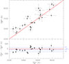 |
Fig. 1. Upper panel: comparison between effective temperatures derived from spectroscopy and photometry. The solid red solid represents the bisecting line. Bottom panel: residuals, computed as |

Derived atmospheric parameters for the sample of classical Cepheids.
To further validate our adopted temperatures, we compared our spectroscopic Teff estimates with values from optical spectroscopic studies for a subset of stars in common with the works by Kovtyukh et al. (2005), Luck (2018), and Luck & Andrievsky (2004). For each comparison, we selected the literature value corresponding to the pulsation phase closest to our observation, taking into account differences in period and epoch definitions among the various datasets. The comparison is shown in Fig. 2, where we plot the temperature differences (this work minus the literature) for each star. The agreement is generally good across the sample, which confirms the reliability of our spectroscopic determinations. The only noticeable deviation is derived for X Pup, which shows a larger discrepancy, but still within ∼2σ from literature values. This offset may stem from residual uncertainties in the phase alignment between our observations and those from the literature, as small shifts in pulsation phase can significantly affect Teff estimates in Cepheids.
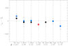 |
Fig. 2. Comparison between the effective temperatures derived in this work (via LDRs) and those from optical spectroscopic studies available in the literature for selected Cepheids. The plot shows the difference |

The determination of surface gravity (log g) and microturbulent velocity (ξ) in our NIR analysis presents specific challenges. In the optical domain, log g is typically constrained by enforcing ionization equilibrium between Fe I and Fe II lines. The NIR spectral window lacks suitable Fe II lines, however, making this direct method unfeasible. Similarly, a reliable spectroscopic determination of ξ from NIR spectra is compromised by the prevalence of saturated lines, which weakens the sensitivity of the line strength to the microturbulence parameter.
To overcome these limitations, we adopted well-established empirical and statistical approaches. For log g, we used the calibrated relation from Elgueta (2021) and Matsunaga et al. (2023),
 (1)
(1)
This relation is based on a large sample of well-characterised Cepheids from Luck (2018) and shows minimal dispersion (0.108 dex), providing a robust and consistent estimate. For the microturbulence, we employed a statistical constraint derived from the full C-MetaLL sample of 538 spectra of classical Cepheids analyzed so far by us (Ripepi et al. 2021; Trentin et al. 2023, 2024). The distribution of ξ measurements was fit with a Gaussian profile, which yielded a characteristic value of ξ = 3.3 ± 0.6 km s−1 (see Fig. 3), which we adopted for all stars in the sample.
 |
Fig. 3. Distribution of microturbulence velocities for the sample of 538 classical Cepheids from the C-MetaLL survey. The Gaussian fit to the distribution yields ξ = 3.3 ± 0.6 km s−1, as labeled. |
To assess the effect of this assumption, we recalculated the iron abundances for two representative stars (SV Vul and X Pup) using alternative values of ξ equal to 2.3 and 4.3 km s−1. Figure 4 shows that the resulting abundance differences are always below 0.1 dex and fall within the typical uncertainties of our measurements. This confirms that adopting a fixed microturbulent velocity does not significantly affect our abundance results and supports the validity of our approach in the context of NIR analyses.
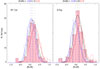 |
Fig. 4. Effect of microturbulent velocity on the derived FeI abundances for two representative stars in the sample, SV Vul and X Pup. Each panel shows the abundance distributions obtained by adopting three different values of ξ: 3.3 km s−1 (pink histogram with the black Gaussian fit), 2.3 km s−1 (red), and 4.3 km s−1 (blue). In all cases, the resulting differences are smaller than 0.1 dex and lie within the typical abundance uncertainties, supporting the robustness of using a fixed ξ in our analysis. |
We acknowledge that these indirect approaches are a limitation of NIR-based analyses compared to the more direct methods available in the optical. The consistency of our final atmospheric parameters and the resulting abundances with extensive optical studies (see Sect. 5) validates our method, however. The excellent agreement in the derived abundance gradients and individual element trends demonstrates that these adopted values for log g and ξ do not introduce significant systematic biases and are appropriate for a homogeneous NIR abundance analysis of Cepheids.
Finally, we determined the spectral broadening (vbroad) through synthetic spectral fitting of multiple Fe I features. The synthetic spectra were convolved with Gaussian profiles of varying widths and compared to the observed line shapes. The resulting atmospheric parameters (Teff, log g, vbroad) for all program stars are compiled in Table 2.
4. Abundances
To mitigate spectral line blending and broadening effects, we employed spectral synthesis techniques. Synthetic spectra were generated through a three-step process:
-
Atmospheric modeling: Plane-parallel local thermodynamic equilibrium (LTE) atmospheric structures were computed using ATLAS9 (Kurucz 1993), initialized with stellar parameters from Table 2.
-
Spectral synthesis: Synthetic spectra were generated with SYNTHE (Kurucz & Avrett 1981). The line lists and atomic parameters we adopted mainly originate from Castelli & Hubrig (2004), which provides updated oscillator strengths (log gf) and damping constants for the compilation of Kurucz (1995). These were supplemented with data from VALD3 (Piskunov et al. 1995) and cross-verified against the APOGEE DR16 line list (Smith et al. 2021). This multi-source approach ensured completeness for NIR diagnostics and consistency in damping treatments. Finally, the spectral lines we selected together with their atomic parameters are provided in Table 3, available in electronic form at the CDS.
-
Broadening convolution: Synthetic spectra were convolved with Gaussian kernels to match instrumental resolution (R ∼ 45 000) and velocity broadening (including rotational and macroturbulent velocities), optimized by fitting unblended metal lines.
The abundances were derived for 16 elements (C, N, Na, Mg, Al, Si, P, S, K, Ca, Ti, Mn, Fe, Ni, Ce, and Yb) using a χ2 minimization. In particular, the spectra were divided into 25–50 Å intervals, and the abundance solutions were obtained by minimizing
![Mathematical equation: $$ \begin{aligned} \chi ^2 = \sum _{i = 1}^{n} { w}_i^2\left[ F_{\text{ obs}}(\lambda _i) - F_{\text{ synth}},(\lambda _i, A) \right]^2, \end{aligned} $$](/articles/aa/full_html/2026/02/aa58020-25/aa58020-25-eq8.gif)
where A is the elemental abundance and wi = 1/σi are the weights associated with the Fobs(λi) (i.e., signal-to-noise ratio S/N). The IDL implementation of the AMOEBA algorithm (Press et al. 1992) performed the optimization. The final abundances represent the median of all valid solutions per element.
The uncertainties were estimated via Monte Carlo simulation, perturbing the continuum placement (±0.5%) and atmospheric parameters within the errors (Teff ± 150 K, log g ± 0.15 dex). The 1σ dispersion of the resulting abundance distributions defined our reported errors. These simulations indicate a typical uncertainty contribution of ± 0.1 dex. Then, the total errors were evaluated by summing the value obtained by the error propagation and the standard deviations obtained from the average abundances in quadrature. For elements with only one measurable spectral line (e.g., phosphorus), we were unable to estimate the dispersion from multiple lines. In these cases, we conservatively adopted the maximum uncertainty derived from the error propagation on the stellar parameters, which amounts to ≈0.15 dex. The final list of LTE abundances for all stars is provided in Table 4, available in electronic form at the CDS. All abundances are referred to the solar value (Grevesse et al. 2011).
Our abundance analysis was based on the assumption of local thermodynamic equilibrium (LTE). While non-LTE (NLTE) effects can impact certain elements, particularly in the infrared (IR) domain, this assumption remains justified for our study based on several lines of evidence. The Cepheids in our sample span effective temperatures of Teff ≈ 4800 – 6200 K and metallicities −0.4 ≤ [Fe/H] ≤ 0.3 dex, which is well within the stellar parameter range explored in recent NLTE studies of cool giants.
In particular, Amarsi et al. (2020) and Lind et al. (2022) showed that NLTE corrections for elements such as Si, Ca, Ti, and Fe are negligible (≤0.05 dex) in this regime. For Na, Mg, and Al (elements for which we used NIR transitions partially in common with the lines analyzed in Lind et al. (2022)), the reported NLTE–LTE abundance differences for solar metallicity stars and mild subgiants mostly remain below 0.1 dex. Stronger NLTE effects (up to ≈0.3 dex) are found for some Al lines beyond 2.1 μm, which we flagged as less reliable. Similarly, Korotin et al. (2020) quantified NLTE corrections for a set of IR transitions in Na, Mg, Al, S, and K for stars with metallicities similar to our targets. They reported typical corrections of ≤0.07 dex for all elements except K, for which NLTE effects can reach ≈0.2 dex.
Based on these findings, and because our analysis is based on differential abundances with respect to the Sun, the systematic impact of NLTE effects on our overall abundance patterns and Galactic gradients is expected to be limited. This is also supported by the strong agreement found between our IGRINS-based abundances and those derived from optical often NLTE-corrected analyses (see Sect. 5).
We therefore conclude that the LTE approximation, while not perfect, remains appropriate within the scope and precision of our analysis. A more detailed NLTE treatment will be explored in a forthcoming paper. Figure 5 shows a representative example of our observed (black) and best-fit synthetic (red) spectrum that illustrates some of the identified lines in the range λ 22 450–22 750 Å.
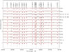 |
Fig. 5. Representative subsample of 13 observed spectra (black) in the region between λ = 22 450 and 22 750 Å. The best-fitting synthetic spectra are overplotted in red. The spectra are ordered from top to bottom by decreasing effective temperature (see Table 2). The main spectral lines are identified at the top and are highlighted with dotted vertical black lines. |
5. Results
We present the chemical abundance results derived from the high-resolution IGRINS spectra of 23 classical Cepheids. The analysis focused on elements that are commonly studied in the optical domain (e.g., Fe, Mg, and Si), which enable a direct comparisons, and on species that are primarily accessible in the NIR (e.g., P, K, and Yb).
Figure 6 shows the radial Galactocentric gradients. The distances were estimated following the procedure described by Gaia Collaboration (2023) and Ripepi et al. (2022a) and used in other works of the C-MetaLL project. We calculated the apparent Wesenheit magnitude W = G − 1.90 × (GBP − GRP) using the Gaia photometry (Ripepi et al. 2019) and the absolute W magnitude from the PWZ relation W = ( − 5.988 ± 0.018)−(3.176 ± 0.044)(log P − 1)−(0.520 ± 0.09)[Fe/H] (Ripepi et al. 2022a). From these two relations, we obtained the distance modulus and then the distance. The new measurements broadly follow the trends established by previous optical studies, which confirms the negative abundance gradients across the Galactic disk. In particular, the slopes derived by Trentin et al. (2024) for [Fe/H], [Mg/H], and [Si/H] are −0.064, −0.055, and −0.049 dex kpc−1, respectively, and our data are fully consistent with these values. Although the radial coverage is comparable to that of previous studies, our analysis provides an independent validation of these trends based on near-infrared H- and K-band spectroscopy with IGRINS. This supports the reliability of abundance determinations in different spectral ranges.
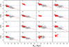 |
Fig. 6. Radial abundance gradients of selected elements in the Galactic disk. The red points represent the Galactic Cepheid abundances we derived from IGRINS H–K spectra, and the gray points correspond to optical measurements from the C-MetaLL sample. The solid red lines indicate the linear fits adopted from Trentin et al. (2024). |
The chemical abundance patterns of our stellar sample are also presented in Fig. 7, where we plot [X/Fe] ratios against metallicity [Fe/H]. The gray points, taken from the C-MetaLL sample, provide a valuable baseline for comparison and establish the general chemical evolution trends in the stellar population.
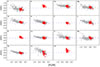 |
Fig. 7. Chemical element abundances (in their [X/Fe] form) plotted against the iron abundance [Fe/H]. The horizontal dashed line at [X/Fe] = 0 indicates the solar abundance ratio. The colors are the same as in Fig. 6. |
Our analysis reveals several key features. The overall trend shows the characteristic decline in [X/Fe] with increasing [Fe/H], consistent with the established scenario of Galactic chemical evolution where Type Ia supernovae begin to contribute significantly to iron production after the initial enrichment by core-collapse supernovae (SNeII). The red points, representing our specific measurements, agree very well with the C-MetaLL trends, which validates our analysis method.
Notably, the spread in [X/Fe] ratios at low metallicities in our data and the C-MetaLL sample reflects the inhomogeneous nature of chemical enrichment in the early Galaxy. The consistency between our results and the optical measurements strengthens the interpretation that these patterns represent genuine features of Galactic chemical evolution and are not analysis artifacts.
To further assess the reliability of our abundance determinations based on NIR spectra, we compared our results with independent measurements available in the literature for the same stars. Figure 8 presents a direct comparison for 12 stars between the abundances derived in this work and those published by Bhardwaj et al. (2023, Fe only) and Trentin et al. (2024, 11 chemical species) based on optical high-resolution spectra obtained with the Echelle SpectroPolarimetric Device for the Observation of Stars (ESPaDOnS4), mounted at the CFHT. ESPaDOnS operates with a spectral resolution of R = 81 000 and covers the wavelength range from 3700 to 10 500 Å.
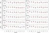 |
Fig. 8. Differences between elemental species (on the x-axis) derived in this work from near-infrared IGRINS spectra (black dots) and those published by T24 using optical high-resolution spectra obtained with ESPaDOnS at the CFHT (red dots). On the y-axis, the difference is expressed in the [X/H] form. Each panel corresponds to a star in common in the two samples. |
The two datasets agree very well in general, with a mean absolute scatter of ≈0.07 dex that is consistent with the typical measurement uncertainties. For iron, we find a negligible median offset of less than 0.02 dex, and the dispersion remains within 0.06 dex. The α-elements magnesium, silicon, and calcium also agree well, with mean differences of 0.05 dex or less and no significant systematic trends. These results confirm that the abundances derived from IGRINS H- and K-band spectra are fully compatible with those obtained from optical spectroscopy, thereby validating the reliability of our near-infrared line selection, model atmospheres, and analysis procedures. This agreement is particularly encouraging for future large-scale abundance studies in the NIR domain, especially where optical data may be inaccessible.
We complemented the comparison shown in Fig. 8 by comparing our abundance determinations with those available in the literature outside the C-MetaLL project. We retrieved abundances from different sources, which implemented independent analyses (e.g., Luck et al. 2011; Luck & Lambert 2011; Genovali et al. 2014, 2015). Figure 9 shows this comparison. These literature studies differ in terms of spectroscopic resolution, wavelength coverage, line selection, and analysis techniques. Despite this methodological diversity, our results agree at 1σ with the published values. Most data points lie close to the null difference line, without significant systematic offsets. This confirms the reliability of our IGRINS-based near-infrared abundance measurements. This agreement, even in an inhomogeneous comparison, reinforces the robustness of our results and their compatibility with optical literature data.
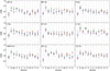 |
Fig. 9. Comparison between elemental abundances derived in this work from IGRINS near-infrared spectra (black circles) and values available in the literature for the same stars. The red asterisks correspond to Luck et al. (2011), blue diamonds to Luck & Lambert (2011), orange squares to Genovali et al. (2014), and green triangles to Genovali et al. (2015). The dashed horizontal blue line marks the null difference. |
In Fig. 10 we compare the nitrogen abundances we derived with near-infrared IGRINS spectra with those published by Luck et al. (2011) for a subset of 18 stars in common. Despite the differences in wavelength domain, instrumentation, and line selection (our abundances are based on the spectral line N I 15852.287 Å and those of Luck et al. (2011) were derived from optical atomic lines), the agreement between the two datasets is remarkably good. The median difference is only +0.03 dex, with a standard deviation of 0.07 dex, well within the expected combined uncertainties. Most points lie close to the one-to-one relation, and no significant trend with abundance level is observed. This level of consistency confirms that reliable nitrogen abundances can be obtained from near-infrared spectra and further supports the robustness of the methodology adopted in this work.
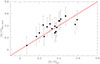 |
Fig. 10. Comparison between nitrogen abundances derived in this work from IGRINS near-infrared spectra (y-axis) with those published by Luck et al. (2011) (x-axis) from optical spectroscopy for 18 stars in common. The solid red line indicates the one-to-one relation. |
6. Discussion
Our study demonstrates that near-infrared spectroscopy with IGRINS provides reliable chemical abundances for well-studied elements and species that are largely inaccessible in the optical domain. The derived α-element gradients (Mg, Si, Ca, and Ti) confirm the well-established negative slopes across the Galactic disk that agrees very well with optical studies. These gradients are a fundamental prediction of inside-out galaxy formation models (e.g. Spitoni et al. 2019; Grisoni et al. 2018), in which the inner disk forms stars more rapidly and efficiently, which leads to earlier and more pronounced enrichment by SNeII. The consistency of our NIR-based gradients with those from optical studies and with chemo-dynamical models provides an independent validation of these theoretical frameworks. It also underscores that NIR spectroscopy is a powerful and reliable tool for probing Galactic chemical evolution, even in regions in which optical data are limited by extinction.
In addition to the α-elements, our IGRINS spectra enable the study of potassium, which occupies an intermediate position between the light α-elements and the heavier neutron-capture species. The [K/H] abundances derived from the NIR lines are mildly correlated with [Fe/H], consistent with the behavior expected for an element that is mainly produced in massive stars and is released into the interstellar medium by SNeII. The lack of significant deviations from the solar-scaled trend suggests that Cepheids accurately trace the present-day potassium content of the Galactic thin disk. This behavior supports theoretical predictions that K nucleosynthesis is sensitive to the progenitor mass and explosion energy, with possible contributions from explosive burning in oxygen- and neon-rich layers (e.g. Kobayashi et al. 2011). Our results identify potassium as a valuable diagnostic element that bridges the information provided by α-elements and heavier r- and s-process tracers such as Yb.
A key advancement of this work is the first homogeneous determination of phosphorus and ytterbium abundances in Cepheids from NIR lines. Our phosphorus measurements, obtained from the P I line at 16482.92 Å in the H band, are consistent with the method of recent high-resolution NIR studies. The work on K giants by Nandakumar et al. (2022), who also used IGRINS, revealed a clear decreasing trend of [P/Fe] with increasing [Fe/H] for disk stars. This behavior is similar to that of α-elements such as Mg and Si and supports a primary nucleosynthetic origin in SNeII that is likely associated with the α-rich freeze-out process (Timmes et al. 1995; Cescutti et al. 2012). Recent calibrations of YJ-band P lines in Cepheids (Elgueta et al. 2024) further highlight the potential of NIR diagnostics for this element. The successful measurement of phosphorus in our Cepheid sample, despite challenges such as telluric contamination and line blending, validates the use of this infrared feature for reliable abundance determinations in luminous pulsating stars.
Ytterbium exhibits a more complex behavior. The derived [Yb/Fe] ratios indicate a dominant r-process contribution (≈60%), as suggested by their similarity to the [Eu/Fe] trend (Montelius et al. 2022). The relatively high [Yb/H] values observed in some disk stars imply a non-negligible s-process component from asymptotic giant branch stars, however. This dual origin makes Yb a powerful diagnostic for disentangling the relative contributions of rapid (neutron star mergers or core-collapse SNe) and slow (AGB) neutron-capture processes to the chemical enrichment of the young Galactic disk. The agreement between our Cepheid Yb abundances and those measured in K giants (Montelius et al. 2022) confirms that NIR lines can reliably trace this complex element in different stellar populations.
By combining the classical α-elements, which trace the yields of core-collapse supernovae, with P (a specific SNeII product), K (a transitional element with explosive nucleosynthetic origin), and Yb (a mixed r- and s-process tracer), our NIR study provides a holistic view of nucleosynthesis in the Galactic disk. The fact that the chemical patterns of Cepheids, which are representatives of the young stellar population, are consistent with those of older K giants suggests that the main production channels for these elements have remained relatively stable throughout the recent history of the disk. Subtle differences in the [Yb/Fe] trend at high metallicity might offer future constraints on the delay-time distribution of r-process events, however.
Finally, the IGRINS observations of the two Cepheids in the LMC, OGLE LMC-CEP-0512 and OGLE LMC-CEP-0992, represent the first high-resolution NIR spectroscopic analysis of these fundamental variables in an external galaxy. These two stars were also analyzed in the optical by Romaniello et al. (2022), allowing for a direct and robust comparison between NIR and optical abundance determinations. The [Fe/H] values we derived (−0.39 and −0.31 dex, respectively) are fully consistent with their optical metallicities, which provides a strong validation of the reliability of NIR-based abundance measurements in low-metallicity extragalactic environments.
7. Conclusions
We presented a detailed chemical analysis of 23 classical Cepheids observed in the H and K bands with the high-resolution spectrograph IGRINS. From these data, we derived atmospheric parameters and abundances for 16 chemical species. The effective temperatures obtained from near-infrared line-depth ratios agree very well with photometric estimates and confirm the reliability of this method for pulsating variable stars.
The abundances derived from the near-infrared spectra are fully consistent with those obtained from optical high-resolution studies, with negligible offsets and dispersions within the observational uncertainties. The α-elements (Mg, Si, Ca, and Ti) display negative radial gradients across the Galactic disk that are consistent with previous optical results and with chemo-dynamical models predicting an inside-out formation of the Milky Way. This agreement validates the use of near-infrared spectroscopy as a robust tool for tracing the chemical structure of the Galaxy, even in regions in which optical observations are hampered by extinction.
A main outcome of this work is the first homogeneous determination of phosphorus, potassium, and ytterbium abundances in Cepheids from near-infrared spectra. The behaviors of phosphorus and potassium are compatible with production in massive stars and SNeII, while ytterbium traces a combination of r- and s-process enrichment, as expected for neutron-capture elements in the Galactic disk. The ability to measure these elements, which are poorly accessible in the optical range, highlights the unique diagnostic potential of high-resolution NIR spectroscopy.
Overall, our analysis demonstrates that IGRINS is a powerful and reliable instrument for abundance studies in Cepheids. Near-infrared spectroscopy not only confirms large-scale chemical trends previously established in the optical, but also extends these studies to additional nucleosynthetic tracers and to highly obscured regions of the Milky Way and nearby galaxies. This capability paves the way for future large-scale NIR surveys with facilities such as MOONS, ELT, and JWST, which will be essential for mapping the chemo-dynamical evolution of our Galaxy fully.
Data availability
Tables 3 and 4 are available at the CDS via https://cdsarc.cds.unistra.fr/viz-bin/cat/J/A+A/706/A225
Acknowledgments
We acknowledge the suggestions of the anonymous referee; her/his comments helped us to improve the manuscript. We acknowledge the financial support from INAF (Large Grant MOVIE, PI: Marconi). We acknowledge funding from INAF GO-GTO grant 2023 “C-MetaLL – Cepheid metallicity in the Leavitt law” (P.I. V. Ripepi) and Project PRIN MUR 2022 (code 2022ARWP9C) “Early Formation and Evolution of Bulge and HalO (EFEBHO)”, PI: Marconi, M., funded by European Union – Next Generation EU. A.B. thanks the funding from the Anusandhan National Research Foundation (ANRF) under the Prime Minister Early Career Research Grant scheme (ANRF/ECRG/2024/000675/PMS). G.D.S. acknowledges support from the INAF–ASTROFIT fellowship, from Gaia DPAC through INAF and ASI (PI: M. G. Lattanzi), and from INFN (Naples Section) through the QGSKY and Moonlight2 initiatives. This research has made use of the SIMBAD database operated at CDS, Strasbourg, France. This work has made use of data from the European Space Agency (ESA) mission Gaia (https://www.cosmos.esa.int/gaia), processed by the Gaia Data Processing and Analysis Consortium (DPAC, https://www.cosmos.esa.int/web/gaia/dpac/consortium). Funding for the DPAC has been provided by national institutions, in particular, the institutions participating in the Gaia Multilateral Agreement. This research was supported by the Munich Institute for Astro-, Particle and BioPhysics (MIAPbP), which is funded by the Deutsche Forschungsgemeinschaft (DFG, German Research Foundation) under Germanys Excellence Strategy – EXC-2094 – 390783311. This research was supported by the International Space Science Institute (ISSI) in Bern/Beijing through ISSI/ISSI-BJ International Team project ID #24-603 – “EXPANDING Universe” (EXploiting Precision AstroNomical Distance INdicators in the Gaia Universe).
References
- Afşar, M., Bozkurt, Z., Topcu, G. B., et al. 2023, ApJ, 949, 86 [CrossRef] [Google Scholar]
- Amarsi, A. M., Lind, K., Osorio, Y., et al. 2020, A&A, 642, A62 [EDP Sciences] [Google Scholar]
- Andrievsky, S. M., Kovtyukh, V. V., Luck, R. E., et al. 2002, A&A, 392, 491 [NASA ADS] [CrossRef] [EDP Sciences] [Google Scholar]
- Bhardwaj, A., Riess, A. G., Catanzaro, G., et al. 2023, ApJ, 955, L13 [NASA ADS] [CrossRef] [Google Scholar]
- Bhardwaj, A., Ripepi, V., Testa, V., et al. 2024, A&A, 683, A234 [NASA ADS] [CrossRef] [EDP Sciences] [Google Scholar]
- Castelli, F., & Hubrig, S. 2004, A&A, 425, 263 [NASA ADS] [CrossRef] [EDP Sciences] [Google Scholar]
- Cardelli, J. A., Clayton, G. C., & Mathis, J. S. 1989, ApJ, 345, 245 [Google Scholar]
- Cescutti, G., Matteucci, F., Caffau, E., & François, P. 2012, A&A, 540, A33 [NASA ADS] [CrossRef] [EDP Sciences] [Google Scholar]
- Chen, X., Wang, S., Deng, L., et al. 2019, Nat. Astron., 3, 320 [NASA ADS] [CrossRef] [Google Scholar]
- da Silva, R., D’Orazi, V., Palla, M., et al. 2023, A&A, 678, A195 [NASA ADS] [CrossRef] [EDP Sciences] [Google Scholar]
- De Somma, G., Marconi, M., Cassisi, S., et al. 2021, MNRAS, 508, 1473 [NASA ADS] [CrossRef] [Google Scholar]
- De Somma, G., Marconi, M., Ripepi, V., et al. 2025, ApJ, 984, L60 [Google Scholar]
- Drimmel, R., Khanna, S., Poggio, E., & Skowron, D. M. 2025, A&A, 698, A230 [NASA ADS] [CrossRef] [EDP Sciences] [Google Scholar]
- Elgueta, S. S. 2021, Ph.D. Thesis, Instituto de Estudios Astrofisicos / Millennium Institute of Astrophysics [Google Scholar]
- Elgueta, S. S., Matsunaga, N., Jian, M., et al. 2024, MNRAS, 532, 3694 [NASA ADS] [CrossRef] [Google Scholar]
- Freedman, W. L., Madore, B. F., Scowcroft, V., et al. 2011, AJ, 142, 192 [CrossRef] [Google Scholar]
- Gaia Collaboration (Drimmel, R., et al.) 2023, A&A, 674, A37 [CrossRef] [EDP Sciences] [Google Scholar]
- Genovali, K., Lemasle, B., Bono, G., et al. 2014, A&A, 566, A37 [NASA ADS] [CrossRef] [EDP Sciences] [Google Scholar]
- Genovali, K., Lemasle, B., da Silva, R., et al. 2015, A&A, 580, A17 [NASA ADS] [CrossRef] [EDP Sciences] [Google Scholar]
- Grevesse, N., Asplund, M., Sauval, A., & Scott, P. 2011, Can. J. Phys., 89, 327 [NASA ADS] [CrossRef] [Google Scholar]
- Grisoni, V., Spitoni, E., & Matteucci, F. 2018, MNRAS, 481, 2570 [NASA ADS] [Google Scholar]
- Gully-Santiago, M., Wang, W., Deen, C., & Jaffe, D. 2012, SPIE Conf. Ser., 8450, 84502S [NASA ADS] [Google Scholar]
- Inno, L., Urbaneja, M. A., Matsunaga, N., et al. 2019, MNRAS, 482, 83 [Google Scholar]
- Jeong, U., Chun, M.-Y., Oh, J. S., et al. 2014, SPIE Conf. Ser., 9154, 91541X [NASA ADS] [Google Scholar]
- Kobayashi, C., Karakas, A. I., & Umeda, H. 2011, MNRAS, 414, 3231 [Google Scholar]
- Korotin, S. A., Andrievsky, S. M., Caffau, E., Bonifacio, P., & Oliva, E. 2020, MNRAS, 496, 2462 [NASA ADS] [CrossRef] [Google Scholar]
- Kovtyukh, V. V., Andrievsky, S. M., Belik, S. I., & Luck, R. E. 2005, AJ, 129, 433 [Google Scholar]
- Kovtyukh, V., Lemasle, B., Bono, G., et al. 2022, MNRAS, 510, 1894 [Google Scholar]
- Kurucz, R. 1995, Atomic Line List [Google Scholar]
- Kurucz, R. L. 1993, International Astronomical Union Colloquium (Cambridge: Cambridge University Press), 138, 87 [Google Scholar]
- Kurucz, R. L., & Avrett, E. H. 1981, SAO Special Report, 391 [Google Scholar]
- Leavitt, H. S., & Pickering, E. C. 1912, Harvard College Observatory Circular, 173, 1 [Google Scholar]
- Lee, J. J., Gullikson, K., & Kaplan, K. 2017, https://doi.org/10.5281/zenodo.845059 [Google Scholar]
- Lemasle, B., Hajdu, G., Kovtyukh, V., et al. 2018, A&A, 618, A160 [NASA ADS] [CrossRef] [EDP Sciences] [Google Scholar]
- Lemasle, B., Lala, H. N., Kovtyukh, V., et al. 2022, A&A, 668, A40 [NASA ADS] [CrossRef] [EDP Sciences] [Google Scholar]
- Lind, K., Nordlander, T., Wehrhahn, A., et al. 2022, A&A, 665, A33 [NASA ADS] [CrossRef] [EDP Sciences] [Google Scholar]
- Luck, R. E. 2018, AJ, 156, 171 [Google Scholar]
- Luck, R. E., & Andrievsky, S. M. 2004, AJ, 128, 343 [Google Scholar]
- Luck, R. E., Andrievsky, S. M., Kovtyukh, V. V., Gieren, W., & Graczyk, D. 2011, AJ, 142, 51 [NASA ADS] [CrossRef] [Google Scholar]
- Luck, R. E., & Lambert, D. L. 2011, AJ, 142, 136 [Google Scholar]
- Mace, G., Kim, H., Jaffe, D. T., et al. 2016, SPIE Conf. Ser., 9908, 99080C [NASA ADS] [Google Scholar]
- Mace, G., Sokal, K., Lee, J.-J., et al. 2018, SPIE Conf. Ser., 10702, 107020Q [NASA ADS] [Google Scholar]
- Madore, B. F. 1982, ApJ, 253, 575 [NASA ADS] [CrossRef] [Google Scholar]
- Marconi, M., De Somma, G., Ripepi, V., et al. 2020, ApJ, 898, L7 [Google Scholar]
- Matsunaga, N., Taniguchi, D., Elgueta, S. S., et al. 2023, ApJ, 954, 198 [NASA ADS] [CrossRef] [Google Scholar]
- Montelius, M., Forsberg, R., Ryde, N., et al. 2022, A&A, 665, A135 [NASA ADS] [CrossRef] [EDP Sciences] [Google Scholar]
- Moon, B., Wang, W., Park, C., et al. 2012, SPIE Conf. Ser., 8450, 845048 [NASA ADS] [Google Scholar]
- Mucciarelli, A., Bellazzini, M., & Massari, D. 2021, A&A, 653, A90 [NASA ADS] [CrossRef] [EDP Sciences] [Google Scholar]
- Nandakumar, G., Ryde, N., Montelius, M., et al. 2022, A&A, 668, A88 [NASA ADS] [CrossRef] [EDP Sciences] [Google Scholar]
- Park, C., Jaffe, D. T., Yuk, I.-S., et al. 2014, SPIE Conf. Ser., 9147, 91471D [NASA ADS] [Google Scholar]
- Pedicelli, S., Bono, G., Lemasle, B., et al. 2009, A&A, 504, 81 [NASA ADS] [CrossRef] [EDP Sciences] [Google Scholar]
- Piskunov, N. E., Kupka, F., Ryabchikova, T. A., Weiss, W. W., & Jeffery, C. S. 1995, A&AS, 112, 525 [Google Scholar]
- Poggio, E., Drimmel, R., Cantat-Gaudin, T., et al. 2021, A&A, 651, A104 [NASA ADS] [CrossRef] [EDP Sciences] [Google Scholar]
- Press, W. H., Teukolsky, S. A., Vetterling, W. T., & Flannery, B. P. 1992, Numerical Recipes in C (Cambridge: Cambridge University Press) [Google Scholar]
- Riess, A. G., Macri, L. M., Hoffmann, S. L., et al. 2016, ApJ, 826, 56 [Google Scholar]
- Riess, A. G., Casertano, S., Yuan, W., et al. 2021, ApJ, 908, L6 [NASA ADS] [CrossRef] [Google Scholar]
- Ripepi, V., Cioni, M.-R. L., Moretti, M. I., et al. 2017, MNRAS, 472, 808 [Google Scholar]
- Ripepi, V., Molinaro, R., Musella, I., et al. 2019, A&A, 625, A14 [NASA ADS] [CrossRef] [EDP Sciences] [Google Scholar]
- Ripepi, V., Catanzaro, G., Molinaro, R., et al. 2021, MNRAS, 508, 4047 [NASA ADS] [CrossRef] [Google Scholar]
- Ripepi, V., Catanzaro, G., Clementini, G., et al. 2022a, A&A, 659, A167 [NASA ADS] [CrossRef] [EDP Sciences] [Google Scholar]
- Ripepi, V., Chemin, L., Molinaro, R., et al. 2022b, MNRAS, 512, 563 [NASA ADS] [CrossRef] [Google Scholar]
- Ripepi, V., Trentin, E., Catanzaro, G., et al. 2025, A&A, submitted [arXiv:2508.17447] [Google Scholar]
- Romaniello, M., Riess, A., Mancino, S., et al. 2022, A&A, 658, A29 [NASA ADS] [CrossRef] [EDP Sciences] [Google Scholar]
- Skowron, D. M., Skowron, J., Mróz, P., et al. 2019, Science, 365, 478 [Google Scholar]
- Smith, V. V., Allende Prieto, C., Beers, T. C., et al. 2021, ApJS, 257, 1 [CrossRef] [Google Scholar]
- Spitoni, E., Silva Aguirre, V., Matteucci, F., Calura, F., & Grisoni, V. 2019, A&A, 623, A60 [NASA ADS] [CrossRef] [EDP Sciences] [Google Scholar]
- Subramanian, S., & Subramaniam, A. 2015, A&A, 573, A135 [NASA ADS] [CrossRef] [EDP Sciences] [Google Scholar]
- Timmes, F. X., Woosley, S. E., & Weaver, T. A. 1995, ApJS, 98, 617 [NASA ADS] [CrossRef] [Google Scholar]
- Trentin, E., Ripepi, V., Catanzaro, G., et al. 2023, MNRAS, 519, 2331 [Google Scholar]
- Trentin, E., Catanzaro, G., Ripepi, V., et al. 2024, A&A, 690, A246 [NASA ADS] [CrossRef] [EDP Sciences] [Google Scholar]
- Yuk, I.-S., Jaffe, D. T., Barnes, S., et al. 2010, SPIE Conf. Ser., 7735, 77351M [NASA ADS] [Google Scholar]
The Wesenheit magnitude is reddening-free by construction, as long as the reddening law is known (Madore 1982).
PI: Bhardwaj, GS-2021-Q-218.
All Tables
All Figures
|
Fig. 1. Upper panel: comparison between effective temperatures derived from spectroscopy and photometry. The solid red solid represents the bisecting line. Bottom panel: residuals, computed as |
| In the text | |
|
Fig. 2. Comparison between the effective temperatures derived in this work (via LDRs) and those from optical spectroscopic studies available in the literature for selected Cepheids. The plot shows the difference |
| In the text | |
|
Fig. 3. Distribution of microturbulence velocities for the sample of 538 classical Cepheids from the C-MetaLL survey. The Gaussian fit to the distribution yields ξ = 3.3 ± 0.6 km s−1, as labeled. |
| In the text | |
|
Fig. 4. Effect of microturbulent velocity on the derived FeI abundances for two representative stars in the sample, SV Vul and X Pup. Each panel shows the abundance distributions obtained by adopting three different values of ξ: 3.3 km s−1 (pink histogram with the black Gaussian fit), 2.3 km s−1 (red), and 4.3 km s−1 (blue). In all cases, the resulting differences are smaller than 0.1 dex and lie within the typical abundance uncertainties, supporting the robustness of using a fixed ξ in our analysis. |
| In the text | |
|
Fig. 5. Representative subsample of 13 observed spectra (black) in the region between λ = 22 450 and 22 750 Å. The best-fitting synthetic spectra are overplotted in red. The spectra are ordered from top to bottom by decreasing effective temperature (see Table 2). The main spectral lines are identified at the top and are highlighted with dotted vertical black lines. |
| In the text | |
|
Fig. 6. Radial abundance gradients of selected elements in the Galactic disk. The red points represent the Galactic Cepheid abundances we derived from IGRINS H–K spectra, and the gray points correspond to optical measurements from the C-MetaLL sample. The solid red lines indicate the linear fits adopted from Trentin et al. (2024). |
| In the text | |
|
Fig. 7. Chemical element abundances (in their [X/Fe] form) plotted against the iron abundance [Fe/H]. The horizontal dashed line at [X/Fe] = 0 indicates the solar abundance ratio. The colors are the same as in Fig. 6. |
| In the text | |
|
Fig. 8. Differences between elemental species (on the x-axis) derived in this work from near-infrared IGRINS spectra (black dots) and those published by T24 using optical high-resolution spectra obtained with ESPaDOnS at the CFHT (red dots). On the y-axis, the difference is expressed in the [X/H] form. Each panel corresponds to a star in common in the two samples. |
| In the text | |
|
Fig. 9. Comparison between elemental abundances derived in this work from IGRINS near-infrared spectra (black circles) and values available in the literature for the same stars. The red asterisks correspond to Luck et al. (2011), blue diamonds to Luck & Lambert (2011), orange squares to Genovali et al. (2014), and green triangles to Genovali et al. (2015). The dashed horizontal blue line marks the null difference. |
| In the text | |
|
Fig. 10. Comparison between nitrogen abundances derived in this work from IGRINS near-infrared spectra (y-axis) with those published by Luck et al. (2011) (x-axis) from optical spectroscopy for 18 stars in common. The solid red line indicates the one-to-one relation. |
| In the text | |
Current usage metrics show cumulative count of Article Views (full-text article views including HTML views, PDF and ePub downloads, according to the available data) and Abstracts Views on Vision4Press platform.
Data correspond to usage on the plateform after 2015. The current usage metrics is available 48-96 hours after online publication and is updated daily on week days.
Initial download of the metrics may take a while.