| Issue |
A&A
Volume 706, February 2026
|
|
|---|---|---|
| Article Number | A340 | |
| Number of page(s) | 11 | |
| Section | Cosmology (including clusters of galaxies) | |
| DOI | https://doi.org/10.1051/0004-6361/202558400 | |
| Published online | 19 February 2026 | |
The AIDA-TNG project: 3D halo shapes
1
INAF-Osservatorio di Astrofisica e Scienza dello Spazio di Bologna Via Piero Gobetti 93/3 I-40129 Bologna, Italy
2
INFN – Sezione di Bologna Viale Berti Pichat 6/2 I-40127 Bologna, Italy
3
Dipartimento di Fisica e Astronomia “Augusto Righi”, Alma Mater Studiorum Università di Bologna Via Gobetti 93/2 I-40129 Bologna, Italy
4
Center for Particle Cosmology, University of Pennsylvania Philadelphia PA 19104, USA
5
Max-Planck-Institut für Astronomie Königstuhl 17 D-69117 Heidelberg, Germany
6
Department of Physics, Kavli Institute for Astrophysics and Space Research, Massachusetts Institute of Technology Cambridge MA 02139, USA
★ Corresponding author: This email address is being protected from spambots. You need JavaScript enabled to view it.
Received:
4
December
2025
Accepted:
8
January
2026
Abstract
Context. The shapes of dark matter halos can be used to constrain the fundamental properties of dark matter. In standard cold dark matter (CDM) cosmologies, halos are typically triaxial, with a preference for prolate configurations; however, including the full baryonic physics tends to make them more oblate.
Aims. We focus on the characterization of total matter 3D shapes in alternative dark matter models, such as self-interacting dark matter (SIDM) and warm dark matter (WDM). These scenarios predict different structural properties due to collisional effects or the suppression of small-scale power.
Methods. We measured the different halo component shapes – dark matter, stars, and gas – at various radii from the center in AIDA-TNG (Alternative Interacting Dark Matter and Astrophysics – TNG), which is a suite of high-resolution cosmological simulations built upon the IllustrisTNG framework. The intent was to systematically study how different dark matter models – specifically SIDM and WDM – affect galaxy formation and the structure of dark matter halos when realistic baryonic physics is included.
Results. SIDM models tend to produce rounder and more isotropic halos, especially in the inner regions, as a result of momentum exchange between dark matter particles. Group- and cluster-size WDM halos are also slightly more spherical than their CDM counterparts. In all cases, the inclusion of self-consistent baryonic physics makes the central regions of all halos rounder, while still revealing clear distinctions among the various dark matter models, notably the self-interacting ones.
Conclusions. The general framework presented in this work, based on the 3D halo shape, can be useful for interpreting multiwavelength data analyses of galaxies and clusters.
Key words: gravitation / hydrodynamics / methods: numerical / cosmology: theory / dark matter / large-scale structure of Universe
© The Authors 2026
 Open Access article, published by EDP Sciences, under the terms of the Creative Commons Attribution License (https://creativecommons.org/licenses/by/4.0), which permits unrestricted use, distribution, and reproduction in any medium, provided the original work is properly cited.
This article is published in open access under the Subscribe to Open model. This email address is being protected from spambots. You need JavaScript enabled to view it. to support open access publication.
1. Introduction
The Λ cold dark matter (CDM) model has become the standard paradigm for cosmic structure formation, successfully describing the hierarchical assembly of galaxies and clusters within dark matter (DM) halos (White & Rees 1978; Bond et al. 1991; Tormen et al. 1997; Tormen 1998). In this framework, DM halos arise from the nonlinear growth of primordial density fluctuations (Press & Schechter 1974; Bardeen et al. 1986; Sheth & Tormen 1999; Musso & Sheth 2021), observed in the cosmic microwave background (Planck Collaboration VI 2020), and provide the gravitational potential wells in which baryons condense to form galaxies (Kauffmann & White 1993; White et al. 1996; Bullock et al. 2001; Springel et al. 2005; Baugh 2006). DM constitutes roughly 85% of the total matter density, with baryons contributing the remaining 15%.
Despite its success on large scales, ΛCDM exhibits small-scale tensions, including discrepancies with respect to observational data in central halo densities, shapes, satellite distributions, and velocity anisotropies (Vogelsberger et al. 2012; Weinberg et al. 2015; Vogelsberger et al. 2016; Bullock & Boylan-Kolchin 2017; Zavala & Frenk 2019; Meneghetti et al. 2020). These tensions have motivated the exploration of alternative dark matter (ADM) scenarios, such as self-interacting dark matter (SIDM) and warm dark matter (WDM). SIDM introduces non-negligible particle scattering, which can isotropize orbits, reduce halo triaxiality, and produce cored central density profiles (Rocha et al. 2013; Zavala et al. 2013; Robertson et al. 2018; Vogelsberger et al. 2019; O’Neil et al. 2023). WDM suppresses small-scale power and delays halo formation, leading to less concentrated, more spherical halos compared to CDM (Lovell et al. 2012; Menci et al. 2012). In hierarchical models, the shape and structure of a DM halo can be affected by its assembly history (Jing & Suto 2002; Allgood et al. 2006; Rossi et al. 2011; Despali et al. 2013; Bonamigo et al. 2015; Musso & Sheth 2023; Nikakhtar et al. 2025). Therefore, understanding the effects of ADM models on halo assembly and morphology is critical for interpreting both simulations and observational data (Davé et al. 2001; Viel et al. 2005, 2012, 2013; Kaplinghat et al. 2016; Tulin & Yu 2018).
Hydrodynamical simulations demonstrate that baryonic physics significantly alters halo and subhalo internal structure (Despali & Vegetti 2017). The condensation of baryons into the central region of a halo increases its sphericity and oblateness; stellar and active galactic nucleus (AGN) feedback can partially counteract these effects by redistributing gas and energy (Gnedin et al. 2004; Bryan et al. 2013; Pillepich et al. 2018a; Chua et al. 2019). Halo shapes vary with radius: they are typically more triaxial in the inner regions and rounder near the virial radius (Despali et al. 2013, 2014, 2017). The velocity anisotropies of DM particles and halo stars also depend on the radius: they are nearly isotropic at small radii, increasingly radial at intermediate distances, and sometimes return to isotropy near the virial boundary (Wojtak et al. 2005; Ascasibar & Gottlöber 2008). Baryons reduce radial motions, increase tangential orbit fractions, and raise velocity dispersions, particularly in central regions.
Substructures and anisotropic accretion further influence halo morphology (Nipoti et al. 2018). The infall of massive satellites is typically directed along filaments, while smaller satellites are accreted from a broader range of angles, affecting halo triaxiality in the outskirts (Knebe et al. 2004; Libeskind et al. 2013a,b; Forero-Romero et al. 2014). The combined effects of baryons, substructure, and filamentary accretion produce complex, radially dependent halo shapes. Observational studies infer triaxial halo shapes through gravitational lensing, X-ray measurements, the Sunyaev-Zel’dovich effect, and the spatial distribution of satellites (De Filippis et al. 2005; Oguri et al. 2010; Sereno et al. 2013; Gonzalez et al. 2021). Typically, the observable is a projected 2D shape (Meneghetti et al. 2007b); we defer a detailed study of the inversion of this projection into 2D detectable quantities to a separate paper.
In this work we used the Alternative Interacting Dark Matter and Astrophysics in the TNG universe (AIDA-TNG) simulations (Despali et al. 2025b), a suite of high-resolution cosmological magnetohydrodynamical runs, to explore halos’ 3D shapes and internal properties across CDM, SIDM, and WDM scenarios. The AIDA-TNG simulations incorporate full baryonic physics, including gas cooling, star formation, and feedback processes, allowing us to quantify the interplay between baryons and DM microphysics (Vogelsberger et al. 2014a,b; Rodriguez-Gomez et al. 2016, 2017; Pillepich et al. 2018a; Vogelsberger et al. 2020). The reference dark matter-only (DMO) runs also allowed us to quantify the effects of baryonic physics implementations and possible impacts on DM particle properties. We focused on mass-selected halo samples across different DM models, without attempting direct halo matching, to provide a statistically representative assessment of how halo morphology responds to baryonic processes and ADM properties.
Specifically, we characterized 3D halo shapes using axis ratio parameters and investigated the radial dependence of these properties as a function of the velocity anisotropies of DM particles, gas, and halo stars. We examined the influence of substructure and halo mass on these trends. By comparing CDM, SIDM, and WDM runs, we connected simulation predictions to observable signatures, providing insights relevant for ongoing and upcoming surveys such as Euclid (Laureijs et al. 2011; Euclid Collaboration: Scaramella et al. 2022; Euclid Collaboration: Mellier et al. 2025), DESI (Dark Energy Spectroscopic Instrument)1 (DESI Collaboration 2022), and JWST2 (Mainieri et al. 2024). This study thus advances our understanding of the combined impact of baryons and DM physics on halo structure, with implications for both theoretical and observational aspects.
The structure of this paper is as follows. In Sect. 2 we describe the cosmological simulations employed in this study. In Sect. 3 we present the method used to measure axis ratios and discuss our results as a function of radius, taking the various DM models into consideration. In Sect. 4 we examine the misalignment of the various components, highlighting how it depends on DM particle models. In Sects. 5 and 6 we study the correlation between the major-to-minor axis ratio as a function of the host halo mass and the intermediate-to-minor axis ratio. We summarize and conclude in Sect. 7.
2. AIDA-TNG cosmological hydrodynamical simulations
The AIDA-TNG simulations (Despali et al. 2025a,b; Romanello et al. 2025) consist of three cosmological volumes of increasing resolution and decreasing size simulated in CDM and ADM models, with and without baryonic physics. This work utilizes the largest boxes, measuring 75 h−1 Mpc (110.7 Mpc) on a side (see Table 1 for more details). The uniqueness of the AIDA set lies in the fact that we can utilize the same cosmological volumes across multiple DM scenarios that encompass CDM, WDM, and SIDM. In particular, we made use of the WDM3 run, which corresponds to a particle mass of 3 keV, and two different self-interacting models, namely SIDM1 with a constant cross section equal to 1 cm2 g−1 and vSIDM with a scale-dependent cross section as described in Correa (2021). Moreover, we were able to rely on both a DMO and a full-physics (FP) version of each run in order to disentangle the effects, relative to a standard CDM run, of ADM and baryonic physics as described by the IllustrisTNG galaxy formation model (TNG hereafter; Weinberger et al. 2017; Pillepich et al. 2018a).
The AIDA-TNG runs used in this work.
All simulations started at redshift z = 127 and adopted the cosmological model from Planck Collaboration XXIV (2016): Ωm = 0.3089, ΩΛ = 0.6911, Ωb = 0.0486, H0 = 67.74 km s−1 Mpc, and σ8 = 0.8159. We generated the initial conditions via the N-GENIC code (Springel 2005) by applying the Zel’dovich approximation on a glass distribution of particles with a linear matter transfer function computed using the CAMB code (Lewis et al. 2000). The simulations were run from the same initial conditions as the corresponding runs of the original IllustrisTNG runs (Pillepich et al. 2018b).
Halos and subhalos were identified using a two-step procedure that combines a friends-of-friends (FOF) algorithm with the SUBFIND substructure finder (Davis et al. 1985; Springel et al. 2001; Dolag et al. 2009). In the first step, the FOF algorithm groups DM particles into halos using a standard linking length of b = 0.2 times the mean inter-particle separation, corresponding approximately to an overdensity of ∼200 times the mean cosmic density. This step provides a catalog of virialized structures, each potentially containing multiple gravitationally bound subhalos. In the second step, the SUBFIND algorithm is applied to each FOF group to identify locally overdense and self-bound substructures. The most massive of these is referred to as the “main,” or smooth, subhalo, and is typically associated with the central galaxy, while smaller subhalos correspond to orbiting satellites or infalling systems.
For each particle type – DM, gas, stars, and black holes – SUBFIND determines membership based on local density peaks and gravitational binding energy. The resulting catalogs provide the physical and structural properties (e.g., total mass, stellar mass, gas fraction, and potential minimum) for both the main halo and its substructures. In this work, we based our halo shape analysis on all particles within the virialized region of each FOF group, rather than limiting the study to the main SUBFIND halo, using the minimum of the gravitational potential as the halo center. This choice ensures that the inferred 3D shapes account for the full mass distribution, including substructures and diffuse components, which is essential when comparing different DM models such as CDM, SIDM, and WDM, where subhalo abundance and survival can vary significantly (e.g., Giocoli et al. 2008, 2010; Despali et al. 2022; Ragagnin et al. 2022; Euclid Collaboration: Giocoli et al. 2024; Euclid Collaboration: Ragagnin et al. 2025). For this work, we made use of the particle positions and halo catalogs from the z = 0 snapshot.
3. Global halo shapes
Numerous studies have demonstrated that the density distribution of DM halos is better described by triaxial ellipsoids rather than by assuming spherical symmetry (e.g., Allgood et al. 2006; Peter et al. 2013; Despali et al. 2013, 2017; Chua et al. 2019). This triaxial nature reflects the anisotropic collapse and hierarchical assembly of structures in the cosmic web, where halos accrete matter preferentially along filaments and experience repeated mergers that preserve memory of large-scale anisotropies. Departures from spherical symmetry are therefore a natural outcome of structure formation in a ΛCDM Universe (Sheth et al. 2001; Sheth & Tormen 2002; Musso & Sheth 2021) and can be further modified by baryonic processes and the small-scale properties of DM (Blumenthal et al. 1986; Borgani et al. 2006; Cusworth et al. 2014; Cui et al. 2016).
In Fig. 1 we show the particle distribution in the most massive halo identified at z = 0 in the CDM hydro simulation. While the stars and DM appear clumpy, distributed between the main halo and dense substructure components, the gas is considerably smoother. It is therefore clear that the triaxiality of these components differs significantly, reflecting their distinct dynamical and dissipative properties.
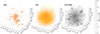 |
Fig. 1. 3D distribution of particles in stars (left), gas (center), and DM (right) of the most massive halo in the CDM simulation at z = 0 (M200 = 2.6 × 10¹⁴ h−1 M⊙). |
3.1. Shape parameters
We used the inertia tensor to determine the shapes of all halos in the simulation, as well as the shapes of their baryonic components: gas and star particles. Commonly, for a system of N particles with masses mi and position vectors xi measured with respect to the halo center, the mass-weighted tensor is defined as
 (1)
(1)
where ri denotes the ellipsoidal distance of each particle from the halo center:
 (2)
(2)
The weighting in the inertial tensor ensures convergence toward a self-consistent ellipsoidal shape (Jing & Suto 2002; Allgood et al. 2006; Zemp et al. 2011). Shape determination is performed iteratively: starting from a spherical volume, the tensor is computed, diagonalized, and the resulting axis ratios are used to redefine the ellipsoidal boundary, enclosing N particles – also updated at each step – until a 1% convergence on the axis ratios is achieved. The resulting axis ratios describe the flattening of the halo (Bardeen et al. 1986; Matarrese et al. 1991). If a ≥ b ≥ c, we define the ellipticity as
![Mathematical equation: $$ \begin{aligned} \epsilon = \dfrac{1-\left(\dfrac{c}{a}\right)^2}{2 \left[ 1 + \left(\dfrac{b}{a}\right)^2 + \left(\dfrac{c}{a}\right)^2 \right]}\,, \end{aligned} $$](/articles/aa/full_html/2026/02/aa58400-25/aa58400-25-eq4.gif) (3)
(3)
and the prolateness as
![Mathematical equation: $$ \begin{aligned} p = \dfrac{1-2 \left(\dfrac{b}{a}\right)^2 + \left(\dfrac{c}{a}\right)^2}{2 \left[ 1 + \left(\dfrac{b}{a}\right)^2 + \left(\dfrac{c}{a}\right)^2 \right]}. \end{aligned} $$](/articles/aa/full_html/2026/02/aa58400-25/aa58400-25-eq5.gif) (4)
(4)
Halos with p > 0 are considered prolate, and halos with p < 0 are oblate. In the limiting cases where p = ϵ and p = −ϵ, one obtains a prolate and an oblate spheroid, respectively. We can also quantify the degree of triaxiality using the parameter,
 (5)
(5)
where T = 0 corresponds to a perfectly oblate spheroid, T = 1 to a prolate spheroid, and intermediate values indicate triaxial configurations (Franx et al. 1991; Bett et al. 2007; Despali et al. 2013). Typically, halos with T < 0.33 are classified as oblate, those with T > 0.67 as prolate, and the rest as triaxial. These quantities provide self-consistent and reproducible measures of the intrinsic halo geometry, allowing for direct comparisons across simulations with different DM models and baryonic physics implementations. In the context of the AIDA-TNG simulations, we applied this method to quantify the 3D shapes of halos formed under CDM, WDM, and SIDM scenarios, and to investigate how baryonic feedback and DM microphysics jointly affect their morphological evolution.
We computed halo shapes, reading particle positions and accumulating them within 32 concentric radial bins, spaced logarithmically in the interval −2 ≤ log(r/R200)≤0, where R200 represents the radius enclosing 200 times the critical density of the universe. While Despali et al. (2022) restricted their shape measurements to the main smooth halo identified by SUBFIND, we included all particles bound within the virialized region, thereby capturing the full contribution from both the main halo and its substructures. Shape measurements are performed independently at each enclosed radius, allowing the ellipsoid’s axis ratios and orientation to vary freely. To ensure robust shape estimates and define the smallest radius at which we trust the measurements of the various components, a minimum of 64 DM particles per shell is required above 10 times the gravitational softening length of the simulation, following the convergence test done by Chua et al. (2019) – as for the TNG-2 run that has the same resolution as the AIDA-TNG simulations.
We also estimated the shape from the satellite distribution, using the stellar mass as a weight (we require satellites to have at least 32 DM and 10 star particles), without iteration in this case. We only did this on two scales – at R200 and R200/2 – and we only considered enclosed radial bins that have at least eight satellites when estimating the 3D shape.
3.2. Shapes in the CDM model
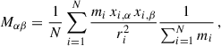
In Fig. 2 we present the median radial profiles of the intermediate-to-major (b/a, top panels) and minor-to-major (c/a, bottom panels) axis ratios for all mass components of halos at z = 0 in the CDM scenario. We considered four distinct mass bins. These profiles illustrate how the 3D morphology of halos varies from the virial radius down to the innermost regions, and how this behavior depends on the baryonic content and feedback processes. In the DMO run we recovered the expected dependence of the axis ratios on distance, with a higher triaxiality toward the halo center (e.g., Allgood et al. 2006; Despali et al. 2017; Chua et al. 2019). Across all mass ranges, the total matter distribution closely follows that of the DM from the virial radius down to approximately half this value, indicating that at these large scales the baryonic component follows the dominant DM potential. However, a mild deviation emerges at smaller radii: the DM becomes slightly more spherical than the total mass distribution. This difference reflects the influence of the dissipative baryonic component, which tends to settle into more compact structures within the central potential well, dominating the total density profile.
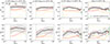 |
Fig. 2. Median profiles of minor-to-major (top) and intermediate-to-major (bottom) axis ratios for z = 0 halos in the CDM simulation in bins of increasing mass (from left to right). Solid black curves show the total axis ratios in the FP run, while solid red, dotted gold, and solid orange curves show the corresponding results for the DM, gas, and stars, respectively. Dashed red curves show halos in the same mass bins but for the DMO run. Green data points (shown only in some of the boxes) include the satellites and were weighted by stellar mass when computing the inertial mass tensor. The error bars bracket 25% and 75% of the distribution. The vertical bars display the resolution limit, which is equal to 10 times the softening length. The number of halos present in the four considered mass bins is 305, 78, 34, and 14, respectively. |
Star particles display more triaxial shapes than the DM at nearly all radii. This enhanced triaxiality likely originates from the complex assembly history of the stellar component, which includes contributions from in situ star formation as well as the accretion of satellite galaxies. The alignment of the stellar component with the underlying DM potential is therefore only partial, consistent with previous findings from hydrodynamical simulations (e.g., Tenneti et al. 2014; Chua et al. 2019). In addition is worth mentioning that baryons make halos rounder and more oblate, and strengthen the alignment between the stellar and DM components (Chua et al. 2022). These effects become more pronounced with increasing stellar-to-halo mass ratio, indicating that systems with higher baryon conversion efficiency experience a stronger modification of their inner potential. This trend agrees with our AIDA–TNG results, where the inner halo becomes progressively more spherical as the baryonic mass fractions increase, highlighting the central role of feedback-regulated galaxy formation in shaping the DM distribution. We discuss this in more detail in the next section.
It is worth noticing that the morphology of the gaseous component within DM halos reflects a complex interplay between gravitational dynamics and baryonic feedback. As shown in the top panels, the minor-to-major axis ratio c/a indicates that gas tends to concentrate toward the center in low-mass halos, resulting in a more oblate configuration. In contrast, in more massive systems, this central condensation is almost completely suppressed, most likely due to the impact of strong AGN feedback that counteracts cooling and prevents gas from accumulating efficiently in the central regions. This transition highlights the competing roles of radiative cooling and feedback in shaping the internal structure of halos across the mass spectrum. It is worth noting that, toward the center, the gas particles tend to follow the stellar shape, concentrated in the central galaxy.
Interestingly, the shapes derived from the spatial distribution of satellite galaxies – green data points with error bars – provide a good proxy for the global halo morphology. This result is particularly relevant for observations, as the spatial anisotropy of satellite systems can be directly measured in galaxy surveys (e.g., Brainerd 2005; Tempel et al. 2015). Therefore, the agreement between the satellite-based and total matter shapes suggests that observational measurements of satellite distributions can be used to constrain the intrinsic triaxiality of DM halos in the real Universe.
Overall, Fig. 2 demonstrates that halo shapes exhibit systematic and physically motivated variations with radius, component, and halo mass. While the anisotropic accretion of DM largely governs the outer regions, the central morphology is strongly modulated by baryonic physics – specifically, cooling, star formation, and feedback – which collectively determine how matter settles into equilibrium within the central potential well.
3.3. The effect of SIDM and WDM on shapes
As discussed by Despali et al. (2022) and Mastromarino et al. (2023), ADM models introduce additional modifications to the picture described above. Self-interactions are expected to lead to isotropic cores, enhancing sphericity within the central regions, while the smoother accretion histories of c halos may result in rounder outer profiles. These distinct morphological imprints provide a promising avenue for discriminating between DM scenarios, particularly when combined with observables sensitive to halo geometry and alignment. In the context of the AIDA-TNG simulations, the consistency of these trends across a wide range of masses and redshifts suggests that halo shape statistics can serve as a robust diagnostic for both baryonic feedback strength and the nature of DM.
In the top panels of Fig. 3, we compare the total minor-to-major axis ratio of the two self-interacting and WDM models with respect to the corresponding CDM reference hydro-run. This comparison offers valuable insights into how both microphysical and astrophysical processes contribute to the overall morphology of halos across different radial scales. As discussed in the previous section, halos are generally more triaxial and elongated in the inner regions, consistent with previous findings from large-volume cosmological runs (e.g., Allgood et al. 2006; Despali et al. 2017; Chua et al. 2019), and small-scale Milky Way-size halos (Chua et al. 2021).
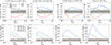 |
Fig. 3. Minor-to-major axis ratios for the DM models relative to the CDM value, for the same (z = 0) mass bins as in Fig. 2. Top and bottom panels display the results from FP and DMO runs, respectively. The dark and light gray shaded regions in all panels indicate 5% and 10% differences, respectively. In dashed red we display the case of the CDM DMO simulation |
In the bottom panels of Fig. 3, we display the relative differences of c/a but for the DMO runs. This can serve as a guide to better understand and quantify the effects of baryonic physics processes that additionally modify the radial profile of the 3D shape of halos of different masses. The changes introduced by ADM and baryons are qualitatively distinct.
Elastic scattering between DM particles transfers momentum and heat within the halo, leading to the formation of a central core and a substantial redistribution of momentum through particle scattering (e.g., Rocha et al. 2013; Spergel & Steinhardt 2000; Robertson et al. 2021). Consequently, SIDM halos are expected to be more spherical than their CDM counterparts, particularly within the inner ∼0.1 R200.
SIDM halos, for both constant and scale-dependent cross sections, are more spherical than CDM in the DMO run (bottom panels of Fig. 3). This trend, albeit diminished, persists when baryons are included, although the combined effect depends on the efficiency of feedback and the characteristic cross section of the interaction. In the top panels of Fig. 3, we see that the baryonic and feedback mechanisms influence and reduce the differences between CDM, SIDM, and vSIDM, especially in the central regions. In all panels, the WDM3 is relatively close, within 5%, to the CDM case. The small differences are due to the small-scale suppression, late forming, and less concentrated WDM halos. For the two highest-mass bins – the last two column subpanels – we can see that at 10% of the halo boundary radius, there is a clear difference between SIDM1 and vSIDM models: the halos in the former are more spherical than in the latter. However, at smaller radii, the behavior changes. While vSIDM halos remain more spherical than their CDM counterparts, SIDM1 halos exhibit shapes that are comparable to those in CDM. These trends are qualitatively similar in the DMO and FP runs, underlining that in the latter, the shape toward the center is more strongly influenced by baryonic physics mechanisms (Despali et al. 2022).
These systematic differences in halo morphology across models have direct observational implications. The 3D shape of DM halos affects gravitational lensing observables, such as the projected ellipticity of convergence maps and the azimuthal variation of weak-lensing shear profiles (e.g., Meneghetti et al. 2001, 2007a; Oguri et al. 2010; Bonamigo et al. 2015; Clampitt & Jain 2016; Despali et al. 2017). Furthermore, the internal alignment between baryonic and DM components influences galaxy–halo misalignment statistics (Piras et al. 2018; Xu et al. 2023a), which can be probed via intrinsic alignment measurements in weak-lensing surveys (Tenneti et al. 2015; Hildebrandt et al. 2017; Heymans et al. 2021; Dark Energy Survey and Kilo-Degree Survey Collaboration 2025). By linking the morphological differences observed in AIDA-TNG to these measurable quantities, we aim to provide a physically motivated framework for interpreting future constraints from high-precision lensing and clustering analyses, and to test the viability of ADM models in the era of Euclid and Rubin.
4. Misalignment angles between star, gas, and dark matter components
The spatial and dynamical alignment between the stellar, DM, and gas components provides an essential diagnostic of halos’ internal structure and assembly history. In ΛCDM cosmologies, the stellar and DM distributions are found to have similar orientations within the central regions, with typical misalignment angles of ∼15 – 30° depending on halo mass, morphology, and feedback strength (e.g., Bett et al. 2010; Velliscig et al. 2015; Chua et al. 2019; Despali et al. 2022). Recent work suggests that the accreted stellar mass fraction is a key factor in determining the misalignment (Xu et al. 2023b). The gas component, being more dynamically responsive to feedback and accretion processes, often shows larger offsets, particularly in systems with strong AGN activity or recent mergers.
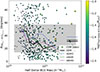 |
Fig. 4. Median misalignment angles, as a function of the rescaled radius, of DM (red) and gas (orange) with respect to the star particles (yellow), in the AIDA-TNG simulations. Dashed, dot-dashed, and dotted lines refer to SIDM1, vSIDM, and WDM3 simulations, respectively, and the four panels are for the same mass bins as in Fig. 2. The colored shaded regions bracket the central 50% (i.e., between 25% and 75%) of the CDM measurements. The four panels represent the four mass bins presented in Fig. 2 |
In the AIDA-TNG simulations, we computed the misalignment between components by measuring the angle between the major axes of the corresponding inertia tensors, derived for the stellar with respect to the DM and gas particle distributions. This was done because we used optically selected stellar components from photometric observations. This approach allowed us to quantify the 3D orientation of each component as a function of radius and halo mass. Results are displayed in Fig. 4.
A systematic difference emerges when comparing self-interacting with CDM models. SIDM halos tend to be more spherical in their inner regions, as frequent DM particle scatterings isotropize the velocity field and redistribute mass (e.g., Rocha et al. 2013; Elbert et al. 2015; Robertson et al. 2021). This enhanced isotropy reduces the coupling between the stellar and DM shapes, resulting in larger misalignment angles in the central regions compared to CDM, particularly in the SIDM1 model. For the same reason, the orientation of the stellar component – largely shaped by baryonic inflows and feedback – is less constrained by the underlying halo. It is worth underlining that the effect is stronger in more massive halos, as shown in the right panels of the figure. Large misalignment angles can also be due to the fact that when shapes are rounder the direction of the axes are less constrained. This is the case for the SIDM1 DM shapes at the high-mass end, as well as for the gas distribution in all mass bins.
The gas component displays a more complex behavior. In massive systems, where AGN feedback dominates, the gas can become uncorrelated with both the stellar and DM components. In contrast, in lower-mass halos, the gas orientation is less misaligned with respect to the overall potential. This results in a weak dependence of the gas–DM misalignment on halo mass but a dependence on the underlying DM model.
Overall, the misalignment statistics provide a complementary probe of the nature of DM and its correlation with the formation processes and assembly histories of halos (Donahue et al. 2016). While CDM predicts a tight alignment between stars and DM, SIDM models naturally produce larger orientation scatter and rounder central morphologies. Future comparisons with observational constraints from weak and strong lensing studies (e.g., Schaller et al. 2015a,b; Harvey et al. 2019, 2021b,a; Robertson et al. 2023) and from integral field spectroscopy of stellar kinematics may therefore help distinguish between these DM scenarios.
In this respect, in Fig. 5, we show the misalignment angle between the brightest central galaxy (BCG) and the host DM halo. We measure this angle between the major axis of the mass tensor ellipsoid, as measured at half-stellar mass and at the halo boundary radius, quantifying how well the central galaxy traces the shape of the host DM halo. The misalignment between the BCG (even when referring to a more general central galaxy) and its host DM halo provides a direct probe of the coupling between baryons and the underlying gravitational potential. In hierarchical structure formation, the major axes of halos and their central galaxies are expected to align along the dominant filamentary accretion direction in the formation phase (e.g., Tenneti et al. 2015; Chisari et al. 2017; Okabe et al. 2020). However, baryonic feedback processes, mergers, and DM self-interactions can perturb this alignment. From the figure, we see that CDM halos tend to be slightly more aligned than the SIDM ones, rounder inner halos, and larger angular offsets due to isotropization of the DM potential (e.g., Harvey et al. 2019; Robertson et al. 2021). The horizontal lines in the right part of the figure mark the median values, over the whole halo sample, of the misalignment angle for the different DM models; precisely equal to 31°, 38°, 34°, and 33° for CDM, SIDM1, vSIDM, and WDM3, respectively. The shaded gray region brackets 50% of the CDM data points. The misalignment is inversely related to the half-stellar mass, the host halo mass M200, and to the ratio between the half stellar mass radius and R200, highlighting that halos that form later have a smaller misalignment between the BCG and host DM halo. From an observational perspective, the distribution of BCG–halo misalignment angles is crucial for interpreting stacked weak-lensing ellipticities and intrinsic alignment statistics in upcoming wide-field weak lensing surveys.
 |
Fig. 5. Misalignment angle between the major axis of the BCG (estimated using the inner 50% of the star particles) and of its host DM halo (estimated from the total mass within R200), shown as a function of half stellar mass of the BCG. Symbol size and color are proportional to the ratio between the central galaxy and host halo sizes for the CDM runs. A dashed gray band encloses 50% of the data points. Black, blue, green, and purple lines show the running median for the CDM, SIDM1, vSIDM, and WDM3 cases, respectively. Horizontal lines on the right indicate the median value, over all half stellar mass values, for the corresponding DM model. |
5. Mass dependence of the minor-to-major axis ratio
The shape of DM halos encodes valuable information on their assembly history and the underlying physical processes that shape their evolution. In this section we present the minor-to-major axis ratio (c/a) of halos as a function of their virial mass, comparing results from the CDM DMO simulation and the FP AIDA-TNG runs.
In the DMO case, the median c/a ratio shows a clear mass dependence, with more massive halos being systematically less spherical. This trend reflects the stronger influence of anisotropic mass accretion and recent mergers in high-mass systems (Allgood et al. 2006; Despali et al. 2014; Bonamigo et al. 2015). Low-mass halos, which typically form earlier and have smoother accretions, have had more time to relax dynamically and therefore display rounder configurations. These results are shown in Fig. 6. Our measurements in the CDM DMO run are in good agreement with the relations derived by Despali et al. (2014) and Bonamigo et al. (2015), confirming that the AIDA-TNG suite reproduces the well-established shape–mass dependence found in previous cosmological simulations.
 |
Fig. 6. Minor-to-major axis ratios as a function of the halo mass (M200). Red data points display the median relation for the CDM DMO simulation at z = 0, while the corresponding solid error bars bracket 25 and 75% of the distribution at fixed halo mass. The connected black, blue, green, and magenta data points show the results for the FP runs in different DM models. To avoid overcrowding, they are displayed without the error bars. The left, central, and right panels show the measurements at the halo boundary radius R200, R200/2, and R200/10, respectively. The dot-dashed green curve shows the results from Despali et al. (2014), while the dotted red and black lines show the best-fit relation assuming the median value of the Bonamigo et al. (2015) model at (c/a)R200 ; this is repeated in all three panels as a guide. |
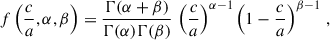
Following Bonamigo et al. (2015), the median relation can be computed from the probability density function for the Beta:
 (6)
(6)
where Γ(x) represents the gamma function3. Bonamigo et al. (2015), using the SBARBINE (Despali et al. 2016) and the Millennium XXL (Angulo et al. 2012) simulations, have shown that the free parameters α and β depend on the peak-height (ν) of the corresponding halo virial mass (Mvir) as follows:
 (7)
(7)
 (8)
(8)
 (9)
(9)
where m = −0.322 and q = 0.620. However, to improve the fit to our DMO and FP CDM simulations, we ran a Markov chain Monte Carlo analysis and let those parameters vary within the ranges [ − 2, −1] and [0, 1], respectively. When converting Mvir to M200, we assumed that halos are described by an NFW profile (Navarro et al. 1996, 1997) with mass and concentration related by the Ludlow et al. (2016) model4. The Bonamigo et al. (2015) model that best fits the DMO CDM simulation at z = 0, with c/a computed at the halo boundary radius (R200), is
 (10)
(10)
for the linear relation parameters in Eq. (9).
Black, blue, green, and magenta symbols (connected by lines), in Fig. 6 show the results of the CDM, SIDM1, vSIDM, and WDM3 hydro runs, respectively. When baryonic physics is included, the halo shapes become significantly rounder, particularly at low and intermediate masses, as well as in the central regions. The median c/a ratio in the FP AIDA-TNG run increases by approximately 15–20% compared to the DMO case, depending on the mass range considered. This sphericalization is a well-known outcome of baryonic condensation in the central regions of halos (e.g., Kazantzidis et al. 2004; Zemp et al. 2011, 2012; Despali et al. 2022). The effect is strongest in halos with M200 ≲ 1013 h−1 M⊙, where stellar and gaseous components dominate the inner potential, while for more massive halos the efficiency of AGN feedback limits baryonic contraction, thereby preserving a more triaxial configuration (Bryan et al. 2013; Butsky et al. 2016; Chua et al. 2019). The best-fit relation for the full-hydro CDM run at z = 0 for c/a measured at R200 is
 (11)
(11)
The comparison between the DMO and FP AIDA-TNG runs suggests that baryonic processes primarily shift the normalization of the c/a–M200 relation upward, rather than altering its slope. This indicates that while the cosmological assembly history drives the overall dependence of halo shape on mass, baryons impose an additional, approximately mass-independent sphericalization effect modulated by feedback strength. This trend is consistent with what has been reported in other large-volume hydrodynamical simulations, such as Illustris and TNG (Chua et al. 2019; Despali et al. 2022).
In addition to baryonic physics, the AIDA-TNG simulations provide an ideal test bed for exploring the impact of ADM models on halo shapes. In particular, the SIDM and WDM runs allow us to disentangle the structural effects of self-interactions and free-streaming suppression from those due to baryonic feedback. As can be seen from Fig. 6, the difference between the various DM models becomes more evident as we move closer to the halo center. In particular, the SIDM models move upward with respect to the CDM model; their halos tend to be more spherical.
In Fig. 7 we show the median minor-to-major axis ratio relation considering only star particles, at R200, R200/2, and R200/10 (left, middle, and right panels, respectively). We can see that star particles at R200 and R200/2 are typically 30% more triaxial than the whole matter, while at 10% of the halo boundary radius – close to the BCG – the star distribution is rounder (axis ratios are closer to unity). The arrows illustrate how much the c/a relation of the total matter must be shifted to describe the stellar minor-to-major axis ratios as a function of halo mass.
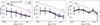 |
Fig. 7. Median minor-to-major axis ratios as a function of the halo mass (M200) considering only star particles for halos at z = 0. The connected black, blue, green, and magenta data points exhibit the results for the FP runs considering different DM models. Error bars bracket 25 and 75% of the distribution, displayed only for the CDM case. The left, central, and right panels show the measurements at the halo boundary radius (R200) and at 50% and 10% of its value, respectively. The dotted black curve shows the recalibrated Bonamigo et al. (2015) model for the (c/a)R200 as measured from all particles in the CDM run. The arrows in each panel indicate the percentage shift of the total-matter c/a relation required to match the minor-to-major axis ratios of the stellar component as a function of halo mass. |
6. Correlation between intermediate and minor axis ratios
The joint distribution of the minor-to-major (c/a) and intermediate-to-major (b/a) axis ratios provides deeper insight into the intrinsic triaxiality of DM halos. While the minor-to-major axis ratio quantifies the overall flattening of a halo, the intermediate-to-major axis ratio captures its degree of prolateness or oblateness. Their correlation thus encodes the balance between anisotropic accretion, mergers, and internal relaxation processes that shape halo morphology (Allgood et al. 2006; Despali et al. 2014; Bonamigo et al. 2015).
In Fig. 8 we show the median distribution of b/a versus c/a for the halos identified in the hydrodynamical and DMO AIDA-TNG runs, measured at R200, R200/2, and R200/10 from left to right. Previous works (Jing & Suto 2002; Rossi et al. 2011) suggested that this relation should be quite universal. We can see that while at R200 the different DM models align within a percent or so, moving toward small radii, the SIDM models deviate with respect to the reference CDM case, while WDM3 remains close to the latter.
 |
Fig. 8. Correlation between the intermediate-to-major and minor-to-major axis ratio for halos at z = 0 in the AIDA-TNG simulation. The left, central, and right panels refer to the correlation measured at the halo boundary radius R200, R200/2, and R200/10, respectively. Shaded contours in the background represent the joint distribution of b/a and c/a (as measured considering all particles within R200 and averaging over all hydrodynamic runs for the different DM models). The blue line shows the median b/a at fixed c/a, with error bars showing the range that encloses 25% of the distribution on either side of this median. The dotted black line shows the corresponding median in the DMO runs. The gray lines refer to the cases of halos with T = 1/3, 2/3, and 1 (top to bottom). The dashed gray line shows the case p = 0, the long-dashed gold curve shows the simplest prediction (for Gaussian initial conditions) described in the text, and the dotted red curve is the relation from Bonamigo et al. (2015). |
The inclusion of baryonic physics significantly alters this relation. In the hydrodynamical AIDA-TNG runs, halos shift toward higher c/a and b/a values, indicating a transition from prolate to more oblate or nearly spherical configurations: the condensation of baryons makes halos rounder and more oblate (Chua et al. 2022). Clearly, halos with c/a ≥ 2/3 lie on the p = 0 relation, whereas those with c/a ≤ 0.5 tend to be prolate rather than triaxial.
The simplest prediction for this relation, based on Gaussian random field statistics, has b/a = 2(c/a)/(1+c/a) (Jing & Suto 2002; Rossi et al. 2011). This tends to overpredict the value of b/a, especially when c/a is small. That is to say, final halo shapes are more prolate than this simplest prediction, suggesting that anisotropic infall along cosmic filaments tends to elongate the halo along the preferred mass accretion direction (e.g., Bett et al. 2007; Vera-Ciro et al. 2011; Bonamigo et al. 2015).
Following Bonamigo et al. (2015), we found that a two-parameter logistic function provides a good fit:
![Mathematical equation: $$ \begin{aligned} \dfrac{b}{a} = 1/\left\{ 1 + \exp {\left[-p_1 \left( \dfrac{c}{a} - p_0\right)\right]}\right\} \,. \end{aligned} $$](/articles/aa/full_html/2026/02/aa58400-25/aa58400-25-eq13.gif) (12)
(12)
In order to compute the best-fit parameters for p0 and p1, we binned all the corresponding DM models – for the DMO and FP runs – along c/a value in 12 bins from 0.1 to 1, computing the median b/a and two percentiles enclosing 25% and 75% of the distribution.
The values for p0 and p1 are reported in Table 2 along with the best-fit reduced chi-squared χν2. For the values computed at the halo boundary R200, the DMO relation is in excellent agreement with the relation reported by Bonamigo et al. (2015), shown here by the dotted red curve.
It is also worth noting that the majority of halos in the figure are triaxial. While the DMO systems are more prolate toward the center, clearly, in the FP AIDA-TNG runs, b/a shifts to larger values when c/a ≥ 0.5, indicating a transition from prolate to more oblate or axisymmetric, if not simply more spherical configurations. This effect is strongest for intermediate-mass systems (M200 ∼ 1012 − 13 h−1 M⊙), where baryonic condensation and feedback efficiently isotropize the potential (Kazantzidis et al. 2004; Butsky et al. 2016; Chua et al. 2019; Despali et al. 2022). Overall, the b/a–c/a relation provides a compact and physically intuitive diagnostic of the mechanisms shaping halo morphology. The comparison across the AIDA-TNG DM models indicates that baryonic physics mainly contribute to halo rounding, albeit through different channels: baryons through dissipative condensation and feedback-induced relaxation, and in addition, SIDM through collisions tend to thermalize the DM component, which is very evident moving toward the halo center. These differences offer an important observational test, as measurements of galaxy and cluster shapes from weak lensing or X-ray isophotes can constrain deviations from triaxiality, thereby providing indirect probes of the DM microphysics (Newman et al. 2013; Duffy et al. 2022; Harvey 2024), as we have shown in the two last sections.
7. Summary and conclusions
In this work we have presented the first analysis of 3D halo shapes, at z = 0, in the AIDA-TNG suite, a set of cosmological hydrodynamical simulations designed to explore how ADM models – CDM, WDM, and SIDM – affect the structure of halos in the presence of realistic baryonic physics. By comparing DMO and FP runs, we quantified how both microphysical interactions and baryonic feedback processes contribute to shaping the internal morphology and alignment of cosmic structures.
Our main results can be summarized as follows:
-
Halo shapes vary systematically with radius and components. The DM dominates and characterizes the overall morphology beyond ∼R200/2, while baryonic condensation and feedback mainly reshape the inner regions. Gas is generally smoother and more oblate, while stars have a more triaxial distribution.
-
Including baryonic physics makes halos significantly rounder than in the DMO case. The degree of sphericalization is largest in low- and intermediate-mass halos, where gas cooling and star formation deepen the potential well, while AGN feedback in massive systems prevents further condensation and maintains the residual triaxiality. In these systems, feedback primarily prevents the inflow of fresh gas rather than erasing the preexisting anisotropies.
-
SIDM models produce rounder, more isotropic inner halos than CDM models due to momentum transfer between DM particles, while WDM halos are both less concentrated and slightly more spherical. The inclusion of baryonic effects reduces but does not eliminate these morphological differences, suggesting that the combined effect of baryonic feedback and DM self-interactions shapes the inner halo structure in a nontrivial manner.
-
The orientation of stars, gas, and DM differs systematically across DM models and halo masses. In CDM, stars are typically aligned within 15–30° with the DM, while SIDM induces larger misalignment angles, especially in massive halos where isotropization weakens the coupling between components. Gas orientations are more sensitive to feedback, becoming uncorrelated with the potential in strongly AGN-dominated systems, and more sensitive to the considered DM model. In addition, we find median misalignments between the BCG and host DM halo – over all halo masses – of 31°, 38°, 34°, and 33° for CDM, SIDM1, vSIDM, and WDM3, respectively. CDM halos are slightly more aligned, while SIDM models show larger offsets due to isotropization of the DM potential. The misalignment decreases with stellar and halo mass, providing a key diagnostic for interpreting weak-lensing ellipticities and intrinsic alignments in upcoming surveys.
-
The minor-to-major axis ratio (c/a) decreases with increasing halo mass, confirming that more massive halos are more triaxial. Baryonic physics results in rounder configurations in which c/a is larger by a mass-independent factor, indicating a nearly mass-independent sphericalization effect. Our results reproduce and extend previous findings (e.g., Despali et al. 2014; Bonamigo et al. 2015) to ADM scenarios.
-
The relation between b/a and c/a follows a tight sequence, with halos being preferentially prolate in the DMO runs and more oblate in the FP case. This transition toward axisymmetry highlights the isotropizing influence of baryonic processes and, to a lesser degree, DM self-interactions. In the FP runs, the central regions tend to be progressively more oblate or spherical; the opposite is true for halos in the DMO simulations.
Overall, our study demonstrates that baryonic feedback remains the dominant driver of halo roundness and alignment in the AIDA-TNG simulations, while ADM physics introduces additional, model-dependent modifications that are most pronounced in the inner regions. The combination of these effects yields distinctive, testable predictions for the 3D morphology of galaxies and clusters. In a recent series of papers, Velmani & Paranjape (2024, 2025) explored physically motivated parameterizations of baryonic feedback and its back-reaction on the DM distribution. We hope our work motivates further studies along these lines that extend beyond the spherical approximation and consider ADM models.
In future work, we will extend our analysis to higher redshifts, exploring the redshift evolution of halo shapes, and link the intrinsic 3D geometry to 2D observable quantities such as weak-lensing ellipticities, X-ray isophotes, and satellite galaxy anisotropies. These comparisons will provide a powerful route to constrain both baryonic feedback efficiency and the fundamental nature of DM.
Acknowledgments
LM and CG acknowledge the financial contribution from the PRIN-MUR 2022 20227RNLY3 grant ‘The concordance cosmological model: stress-tests with galaxy clusters’ supported by Next Generation EU, and from the grant ASI n. 2024-10-HH.0 “Attività scientifiche per la missione Euclid – fase E”. GC thanks the support from INAF theory Grant 2022: Illuminating Dark Matter using Weak Lensing by Cluster Satellites. GD acknowledges the funding by the European Union – NextGenerationEU, in the framework of the HPC project – “National Centre for HPC, Big Data and Quantum Computing” (PNRR – M4C2 – I1.4 – CN00000013 – CUP J33C22001170001). RKS is grateful to the ISA Bologna for support and to the members of DIFA/INAF Bologna for their hospitality in the fall of 2025. We acknowledge the EuroHPC Joint Undertaking for awarding the AIDA-TNG project access to the EuroHPC supercomputer LUMI, hosted by CSC (Finland) and the LUMI consortium through a EuroHPC Extreme Scale Access call. GD acknowledges ISCRA and ICSC for awarding her access to the LEONARDO supercomputer, owned by the EuroHPC Joint Undertaking, hosted by CINECA (Italy).
References
- Allgood, B., Flores, R. A., Primack, J. R., et al. 2006, MNRAS, 367, 1781 [NASA ADS] [CrossRef] [Google Scholar]
- Angulo, R. E., Springel, V., White, S. D. M., et al. 2012, MNRAS, 426, 2046 [NASA ADS] [CrossRef] [Google Scholar]
- Ascasibar, Y., & Gottlöber, S. 2008, MNRAS, 386, 2022 [CrossRef] [Google Scholar]
- Bardeen, J. M., Bond, J. R., Kaiser, N., & Szalay, A. S. 1986, ApJ, 304, 15 [Google Scholar]
- Baugh, C. M. 2006, Rep. Progr. Phys., 69, 3101 [Google Scholar]
- Bett, P., Eke, V., Frenk, C. S., et al. 2007, MNRAS, 376, 215 [NASA ADS] [CrossRef] [Google Scholar]
- Bett, P., Eke, V., Frenk, C. S., Jenkins, A., & Okamoto, T. 2010, MNRAS, 404, 1137 [NASA ADS] [Google Scholar]
- Blumenthal, G. R., Faber, S. M., Flores, R., & Primack, J. R. 1986, ApJ, 301, 27 [Google Scholar]
- Bonamigo, M., Despali, G., Limousin, M., et al. 2015, MNRAS, 449, 3171 [NASA ADS] [CrossRef] [Google Scholar]
- Bond, J. R., Cole, S., Efstathiou, G., & Kaiser, N. 1991, ApJ, 379, 440 [NASA ADS] [CrossRef] [Google Scholar]
- Borgani, S., Dolag, K., Murante, G., et al. 2006, MNRAS, 367, 1641 [NASA ADS] [CrossRef] [Google Scholar]
- Brainerd, T. G. 2005, ApJ, 628, L101 [Google Scholar]
- Bryan, S. E., Kay, S. T., Duffy, A. R., et al. 2013, MNRAS, 429, 3316 [Google Scholar]
- Bullock, J. S., & Boylan-Kolchin, M. 2017, ARA&A, 55, 343 [Google Scholar]
- Bullock, J. S., Kravtsov, A. V., & Weinberg, D. H. 2001, ApJ, 548, 33 [NASA ADS] [CrossRef] [Google Scholar]
- Butsky, I., Macciò, A. V., Dutton, A. A., et al. 2016, MNRAS, 462, 663 [NASA ADS] [CrossRef] [Google Scholar]
- Chisari, N. E., Koukoufilippas, N., Jindal, A., et al. 2017, MNRAS, 472, 1163 [Google Scholar]
- Chua, K. T. E., Pillepich, A., Vogelsberger, M., & Hernquist, L. 2019, MNRAS, 484, 476 [Google Scholar]
- Chua, K. T. E., Dibert, K., Vogelsberger, M., & Zavala, J. 2021, MNRAS, 500, 1531 [NASA ADS] [Google Scholar]
- Chua, K. T. E., Vogelsberger, M., Pillepich, A., & Hernquist, L. 2022, MNRAS, 515, 2681 [NASA ADS] [CrossRef] [Google Scholar]
- Clampitt, J., & Jain, B. 2016, MNRAS, 457, 4135 [Google Scholar]
- Correa, C. A. 2021, MNRAS, 503, 920 [NASA ADS] [CrossRef] [Google Scholar]
- Cui, W., Power, C., Knebe, A., et al. 2016, MNRAS, 458, 4052 [Google Scholar]
- Cusworth, S. J., Kay, S. T., Battye, R. A., & Thomas, P. A. 2014, MNRAS, 439, 2485 [NASA ADS] [CrossRef] [Google Scholar]
- Dark Energy Survey and Kilo-Degree Survey Collaboration (Abbott, T. M. C., et al.) 2023, Open J. Astrophys., 6, 36 [NASA ADS] [Google Scholar]
- Davé, R., Spergel, D. N., Steinhardt, P. J., & Wandelt, B. D. 2001, ApJ, 547, 574 [CrossRef] [Google Scholar]
- Davis, M., Efstathiou, G., Frenk, C. S., & White, S. D. M. 1985, ApJ, 292, 371 [Google Scholar]
- De Filippis, E., Sereno, M., Bautz, M. W., & Longo, G. 2005, ApJ, 625, 108 [NASA ADS] [CrossRef] [Google Scholar]
- DESI Collaboration (Abareshi, B., et al.) 2022, AJ, 164, 207 [NASA ADS] [CrossRef] [Google Scholar]
- Despali, G., & Vegetti, S. 2017, MNRAS, 469, 1997 [NASA ADS] [CrossRef] [Google Scholar]
- Despali, G., Tormen, G., & Sheth, R. K. 2013, MNRAS, 431, 1143 [NASA ADS] [CrossRef] [Google Scholar]
- Despali, G., Giocoli, C., & Tormen, G. 2014, MNRAS, 443, 3208 [Google Scholar]
- Despali, G., Giocoli, C., Angulo, R. E., et al. 2016, MNRAS, 456, 2486 [NASA ADS] [CrossRef] [Google Scholar]
- Despali, G., Giocoli, C., Bonamigo, M., Limousin, M., & Tormen, G. 2017, MNRAS, 466, 181 [Google Scholar]
- Despali, G., Walls, L. G., Vegetti, S., et al. 2022, MNRAS, 516, 4543 [NASA ADS] [CrossRef] [Google Scholar]
- Despali, G., Giocoli, C., Moscardini, L., et al. 2025a, A&A, submitted [arXiv:2512.15869] [Google Scholar]
- Despali, G., Moscardini, L., Nelson, D., et al. 2025b, A&A, 697, A213 [NASA ADS] [CrossRef] [EDP Sciences] [Google Scholar]
- Diemer, B. 2018, ApJS, 239, 35 [NASA ADS] [CrossRef] [Google Scholar]
- Dolag, K., Borgani, S., Murante, G., & Springel, V. 2009, MNRAS, 399, 497 [Google Scholar]
- Donahue, M., Ettori, S., Rasia, E., et al. 2016, ApJ, 819, 36 [Google Scholar]
- Duffy, R. T., Logan, C. H. A., Maughan, B. J., et al. 2022, MNRAS, 512, 2525 [NASA ADS] [CrossRef] [Google Scholar]
- Elbert, O. D., Bullock, J. S., Garrison-Kimmel, S., et al. 2015, MNRAS, 453, 29 [NASA ADS] [CrossRef] [Google Scholar]
- Euclid Collaboration (Scaramella, R., et al.) 2022, A&A, 662, A112 [NASA ADS] [CrossRef] [EDP Sciences] [Google Scholar]
- Euclid Collaboration (Giocoli, C., et al.) 2024, A&A, 681, A67 [NASA ADS] [CrossRef] [EDP Sciences] [Google Scholar]
- Euclid Collaboration (Mellier, Y., et al.) 2025, A&A, 697, A1 [Google Scholar]
- Euclid Collaboration (Ragagnin, A., et al.) 2025, A&A, 695, A282 [Google Scholar]
- Forero-Romero, J. E., Contreras, S., & Padilla, N. 2014, MNRAS, 443, 1090 [NASA ADS] [CrossRef] [Google Scholar]
- Franx, M., Illingworth, G., & de Zeeuw, T. 1991, ApJ, 383, 112 [CrossRef] [Google Scholar]
- Giocoli, C., Tormen, G., Sheth, R. K., & van den Bosch, F. C. 2010, MNRAS, 404, 502 [NASA ADS] [Google Scholar]
- Gnedin, O. Y., Kravtsov, A. V., Klypin, A. A., & Nagai, D. 2004, ApJ, 616, 16 [Google Scholar]
- Giocoli, C., Tormen, G., & van den Bosch, F. C. 2008, MNRAS, 386, 2135 [NASA ADS] [CrossRef] [Google Scholar]
- Gonzalez, E. J., Ragone-Figueroa, C., Donzelli, C. J., et al. 2021, MNRAS, 508, 1280 [Google Scholar]
- Harvey, D. 2024, Nat. Astron., 8, 1332 [Google Scholar]
- Harvey, D., Robertson, A., Massey, R., & McCarthy, I. G. 2019, MNRAS, 488, 1572 [NASA ADS] [CrossRef] [Google Scholar]
- Harvey, D., Chisari, N. E., Robertson, A., & McCarthy, I. G. 2021a, MNRAS, 506, 441 [NASA ADS] [CrossRef] [Google Scholar]
- Harvey, D., Robertson, A., Tam, S.-I., et al. 2021b, MNRAS, 500, 2627 [Google Scholar]
- Heymans, C., Tröster, T., Asgari, M., et al. 2021, A&A, 646, A140 [NASA ADS] [CrossRef] [EDP Sciences] [Google Scholar]
- Hildebrandt, H., Viola, M., Heymans, C., et al. 2017, MNRAS, 465, 1454 [Google Scholar]
- Jing, Y. P., & Suto, Y. 2002, ApJ, 574, 538 [Google Scholar]
- Kaplinghat, M., Tulin, S., & Yu, H.-B. 2016, Phys. Rev. Lett., 116, 041302 [NASA ADS] [CrossRef] [Google Scholar]
- Kauffmann, G., & White, S. D. M. 1993, MNRAS, 261, 921 [Google Scholar]
- Kazantzidis, S., Kravtsov, A. V., Zentner, A. R., et al. 2004, ApJ, 611, L73 [Google Scholar]
- Knebe, A., Gill, S. P. D., Gibson, B. K., et al. 2004, ApJ, 603, 7 [NASA ADS] [CrossRef] [Google Scholar]
- Laureijs, R., Amiaux, J., Arduini, S., et al. 2011, ArXiv e-prints [arXiv:1110.3193] [Google Scholar]
- Lewis, A., Challinor, A., & Lasenby, A. 2000, ApJ, 538, 473 [Google Scholar]
- Libeskind, N. I., Hoffman, Y., Forero-Romero, J., et al. 2013a, MNRAS, 428, 2489 [NASA ADS] [CrossRef] [Google Scholar]
- Libeskind, N. I., Hoffman, Y., Steinmetz, M., et al. 2013b, ApJ, 766, L15 [Google Scholar]
- Lovell, M. R., Eke, V., Frenk, C. S., et al. 2012, MNRAS, 420, 2318 [NASA ADS] [CrossRef] [Google Scholar]
- Ludlow, A. D., Bose, S., Angulo, R. E., et al. 2016, MNRAS, 460, 1214 [Google Scholar]
- Mainieri, V., Anderson, R. I., Brinchmann, J., et al. 2024, ArXiv e-prints [arXiv:2403.05398] [Google Scholar]
- Mastromarino, C., Despali, G., Moscardini, L., et al. 2023, MNRAS, 524, 1515 [NASA ADS] [CrossRef] [Google Scholar]
- Matarrese, S., Lucchin, F., Messina, A., & Moscardini, L. 1991, MNRAS, 253, 35 [Google Scholar]
- Menci, N., Fiore, F., & Lamastra, A. 2012, MNRAS, 421, 2384 [Google Scholar]
- Meneghetti, M., Yoshida, N., Bartelmann, M., et al. 2001, MNRAS, 325, 435 [NASA ADS] [CrossRef] [Google Scholar]
- Meneghetti, M., Bartelmann, M., Jenkins, A., & Frenk, C. 2007a, MNRAS, 381, 171 [Google Scholar]
- Meneghetti, M., Argazzi, R., Pace, F., et al. 2007b, A&A, 461, 25 [NASA ADS] [CrossRef] [EDP Sciences] [Google Scholar]
- Meneghetti, M., Davoli, G., Bergamini, P., et al. 2020, Science, 369, 1347 [Google Scholar]
- Musso, M., & Sheth, R. K. 2021, MNRAS, 508, 3634 [NASA ADS] [CrossRef] [Google Scholar]
- Musso, M., & Sheth, R. K. 2023, MNRAS, 523, L4 [NASA ADS] [CrossRef] [Google Scholar]
- Navarro, J. F., Frenk, C. S., & White, S. D. M. 1996, ApJ, 462, 563 [Google Scholar]
- Navarro, J. F., Frenk, C. S., & White, S. D. M. 1997, ApJ, 490, 493 [Google Scholar]
- Newman, A. B., Treu, T., Ellis, R. S., & Sand, D. J. 2013, ApJ, 765, 25 [NASA ADS] [CrossRef] [Google Scholar]
- Nikakhtar, F., Nagai, D., Musso, M., & Sheth, R. K. 2025, ArXiv e-prints [arXiv:2509.07153] [Google Scholar]
- Nipoti, C., Giocoli, C., & Despali, G. 2018, MNRAS, 476, 705 [Google Scholar]
- Oguri, M., Takada, M., Okabe, N., & Smith, G. P. 2010, MNRAS, 405, 2215 [NASA ADS] [Google Scholar]
- Okabe, T., Nishimichi, T., Oguri, M., et al. 2020, MNRAS, 491, 2268 [Google Scholar]
- O’Neil, S., Vogelsberger, M., Heeba, S., et al. 2023, MNRAS, 524, 288 [Google Scholar]
- Peter, A. H. G., Rocha, M., Bullock, J. S., & Kaplinghat, M. 2013, MNRAS, 430, 105 [Google Scholar]
- Pillepich, A., Nelson, D., Hernquist, L., et al. 2018a, MNRAS, 475, 648 [Google Scholar]
- Pillepich, A., Springel, V., Nelson, D., et al. 2018b, MNRAS, 473, 4077 [Google Scholar]
- Piras, D., Joachimi, B., Schäfer, B. M., et al. 2018, MNRAS, 474, 1165 [Google Scholar]
- Planck Collaboration XXIV. 2016, A&A, 594, A24 [NASA ADS] [CrossRef] [EDP Sciences] [Google Scholar]
- Planck Collaboration VI. 2020, A&A, 641, A6 [NASA ADS] [CrossRef] [EDP Sciences] [Google Scholar]
- Press, W. H., & Schechter, P. 1974, ApJ, 187, 425 [Google Scholar]
- Ragagnin, A., Meneghetti, M., Bassini, L., et al. 2022, A&A, 665, A16 [NASA ADS] [CrossRef] [EDP Sciences] [Google Scholar]
- Robertson, A., Huff, E., & Markovič, K. 2023, MNRAS, 521, 3172 [Google Scholar]
- Robertson, A., Massey, R., Eke, V., Schaye, J., & Theuns, T. 2021, MNRAS, 501, 4610 [NASA ADS] [CrossRef] [Google Scholar]
- Robertson, A., Massey, R., Eke, V., et al. 2018, MNRAS, 476, L20 [Google Scholar]
- Rocha, M., Peter, A. H. G., Bullock, J. S., et al. 2013, MNRAS, 430, 81 [NASA ADS] [CrossRef] [Google Scholar]
- Rodriguez-Gomez, V., Pillepich, A., Sales, L. V., et al. 2016, MNRAS, 458, 2371 [Google Scholar]
- Rodriguez-Gomez, V., Sales, L. V., Genel, S., et al. 2017, MNRAS, 467, 3083 [Google Scholar]
- Romanello, M., Despali, G., Marulli, F., Giocoli, C., & Moscardini, L. 2025, ArXiv e-prints [arXiv:2512.15883] [Google Scholar]
- Rossi, G., Sheth, R. K., & Tormen, G. 2011, MNRAS, 416, 248 [Google Scholar]
- Schaller, M., Frenk, C. S., Bower, R. G., et al. 2015a, MNRAS, 451, 1247 [Google Scholar]
- Schaller, M., Robertson, A., Massey, R., Bower, R. G., & Eke, V. R. 2015b, MNRAS, 453, L58 [Google Scholar]
- Sereno, M., Ettori, S., Umetsu, K., & Baldi, A. 2013, MNRAS, 428, 2241 [NASA ADS] [CrossRef] [Google Scholar]
- Sheth, R. K., Mo, H. J., & Tormen, G. 2001, MNRAS, 323, 1 [NASA ADS] [CrossRef] [Google Scholar]
- Sheth, R. K., & Tormen, G. 1999, MNRAS, 308, 119 [Google Scholar]
- Sheth, R. K., & Tormen, G. 2002, MNRAS, 329, 61 [Google Scholar]
- Spergel, D. N., & Steinhardt, P. J. 2000, Phys. Rev. Lett., 84, 3760 [NASA ADS] [CrossRef] [Google Scholar]
- Springel, V. 2005, MNRAS, 364, 1105 [Google Scholar]
- Springel, V., White, S. D. M., Tormen, G., & Kauffmann, G. 2001, MNRAS, 328, 726 [Google Scholar]
- Springel, V., White, S. D. M., Jenkins, A., et al. 2005, Nature, 435, 629 [Google Scholar]
- Tempel, E., Guo, Q., Kipper, R., & Libeskind, N. I. 2015, MNRAS, 450, 2727 [NASA ADS] [CrossRef] [Google Scholar]
- Tenneti, A., Mandelbaum, R., Di Matteo, T., Feng, Y., & Khandai, N. 2014, MNRAS, 441, 470 [Google Scholar]
- Tenneti, A., Mandelbaum, R., Di Matteo, T., Kiessling, A., & Khandai, N. 2015, MNRAS, 453, 469 [Google Scholar]
- Tormen, G. 1998, MNRAS, 297, 648 [NASA ADS] [CrossRef] [Google Scholar]
- Tormen, G., Bouchet, F. R., & White, S. D. M. 1997, MNRAS, 286, 865 [NASA ADS] [CrossRef] [Google Scholar]
- Tulin, S., & Yu, H.-B. 2018, Phys. Rep., 730, 1 [Google Scholar]
- Velliscig, M., Cacciato, M., Schaye, J., et al. 2015, MNRAS, 454, 3328 [CrossRef] [Google Scholar]
- Velmani, P., & Paranjape, A. 2024, JCAP, 2024, 080 [Google Scholar]
- Velmani, P., & Paranjape, A. 2025, JCAP, 2025, 006 [Google Scholar]
- Vera-Ciro, C. A., Sales, L. V., Helmi, A., et al. 2011, MNRAS, 416, 1377 [NASA ADS] [CrossRef] [Google Scholar]
- Viel, M., Lesgourgues, J., Haehnelt, M. G., Matarrese, S., & Riotto, A. 2005, Phys. Rev. D, 71, 063534 [NASA ADS] [CrossRef] [Google Scholar]
- Viel, M., Becker, G. D., Bolton, J. S., & Haehnelt, M. G. 2013, Phys. Rev. D, 88, 043502 [NASA ADS] [CrossRef] [Google Scholar]
- Viel, M., Markovič, K., Baldi, M., & Weller, J. 2012, MNRAS, 421, 50 [NASA ADS] [Google Scholar]
- Vogelsberger, M., Zavala, J., & Loeb, A. 2012, MNRAS, 423, 3740 [NASA ADS] [CrossRef] [Google Scholar]
- Vogelsberger, M., Genel, S., Springel, V., et al. 2014a, Nature, 509, 177 [Google Scholar]
- Vogelsberger, M., Genel, S., Springel, V., et al. 2014b, MNRAS, 444, 1518 [Google Scholar]
- Vogelsberger, M., Zavala, J., Cyr-Racine, F.-Y., et al. 2016, MNRAS, 460, 1399 [NASA ADS] [CrossRef] [Google Scholar]
- Vogelsberger, M., Zavala, J., Schutz, K., & Slatyer, T. R. 2019, MNRAS, 484, 5437 [NASA ADS] [CrossRef] [Google Scholar]
- Vogelsberger, M., Marinacci, F., Torrey, P., & Puchwein, E. 2020, Nat. Rev. Phys., 2, 42 [Google Scholar]
- Weinberg, D. H., Bullock, J. S., Governato, F., Kuzio de Naray, R., & Peter, A. H. G. 2015, Proc. Natl. Acad. Sci., 112, 12249 [NASA ADS] [CrossRef] [Google Scholar]
- Weinberger, R., Springel, V., Hernquist, L., et al. 2017, MNRAS, 465, 3291 [Google Scholar]
- White, S. D. M. 1996, in Gravitational Dynamics, eds. O. Lahav, E. Terlevich, & R. J. Terlevich, 121 [Google Scholar]
- White, S. D. M., & Rees, M. J. 1978, MNRAS, 183, 341 [Google Scholar]
- Wojtak, R., Łokas, E. L., Gottlöber, S., & Mamon, G. A. 2005, MNRAS, 361, L1 [Google Scholar]
- Xu, K., Jing, Y. P., & Gao, H. 2023a, ApJ, 954, 2 [NASA ADS] [CrossRef] [Google Scholar]
- Xu, K., Jing, Y. P., & Zhao, D. 2023b, ApJ, 957, 45 [NASA ADS] [CrossRef] [Google Scholar]
- Zavala, J., & Frenk, C. S. 2019, Galaxies, 7, 81 [NASA ADS] [CrossRef] [Google Scholar]
- Zavala, J., Vogelsberger, M., & Walker, M. G. 2013, MNRAS, 431, L20 [NASA ADS] [CrossRef] [Google Scholar]
- Zemp, M., Gnedin, O. Y., Gnedin, N. Y., & Kravtsov, A. V. 2011, ApJS, 197, 30 [Google Scholar]
- Zemp, M., Gnedin, O. Y., Gnedin, N. Y., & Kravtsov, A. V. 2012, ApJ, 748, 54 [NASA ADS] [CrossRef] [Google Scholar]
We have computed this using scipy.stats.beta.
In this implementation, we used COLOSSUS (Diemer 2018)
All Tables
All Figures
|
Fig. 1. 3D distribution of particles in stars (left), gas (center), and DM (right) of the most massive halo in the CDM simulation at z = 0 (M200 = 2.6 × 10¹⁴ h−1 M⊙). |
| In the text | |
|
Fig. 2. Median profiles of minor-to-major (top) and intermediate-to-major (bottom) axis ratios for z = 0 halos in the CDM simulation in bins of increasing mass (from left to right). Solid black curves show the total axis ratios in the FP run, while solid red, dotted gold, and solid orange curves show the corresponding results for the DM, gas, and stars, respectively. Dashed red curves show halos in the same mass bins but for the DMO run. Green data points (shown only in some of the boxes) include the satellites and were weighted by stellar mass when computing the inertial mass tensor. The error bars bracket 25% and 75% of the distribution. The vertical bars display the resolution limit, which is equal to 10 times the softening length. The number of halos present in the four considered mass bins is 305, 78, 34, and 14, respectively. |
| In the text | |
|
Fig. 3. Minor-to-major axis ratios for the DM models relative to the CDM value, for the same (z = 0) mass bins as in Fig. 2. Top and bottom panels display the results from FP and DMO runs, respectively. The dark and light gray shaded regions in all panels indicate 5% and 10% differences, respectively. In dashed red we display the case of the CDM DMO simulation |
| In the text | |
|
Fig. 4. Median misalignment angles, as a function of the rescaled radius, of DM (red) and gas (orange) with respect to the star particles (yellow), in the AIDA-TNG simulations. Dashed, dot-dashed, and dotted lines refer to SIDM1, vSIDM, and WDM3 simulations, respectively, and the four panels are for the same mass bins as in Fig. 2. The colored shaded regions bracket the central 50% (i.e., between 25% and 75%) of the CDM measurements. The four panels represent the four mass bins presented in Fig. 2 |
| In the text | |
|
Fig. 5. Misalignment angle between the major axis of the BCG (estimated using the inner 50% of the star particles) and of its host DM halo (estimated from the total mass within R200), shown as a function of half stellar mass of the BCG. Symbol size and color are proportional to the ratio between the central galaxy and host halo sizes for the CDM runs. A dashed gray band encloses 50% of the data points. Black, blue, green, and purple lines show the running median for the CDM, SIDM1, vSIDM, and WDM3 cases, respectively. Horizontal lines on the right indicate the median value, over all half stellar mass values, for the corresponding DM model. |
| In the text | |
|
Fig. 6. Minor-to-major axis ratios as a function of the halo mass (M200). Red data points display the median relation for the CDM DMO simulation at z = 0, while the corresponding solid error bars bracket 25 and 75% of the distribution at fixed halo mass. The connected black, blue, green, and magenta data points show the results for the FP runs in different DM models. To avoid overcrowding, they are displayed without the error bars. The left, central, and right panels show the measurements at the halo boundary radius R200, R200/2, and R200/10, respectively. The dot-dashed green curve shows the results from Despali et al. (2014), while the dotted red and black lines show the best-fit relation assuming the median value of the Bonamigo et al. (2015) model at (c/a)R200 ; this is repeated in all three panels as a guide. |
| In the text | |
|
Fig. 7. Median minor-to-major axis ratios as a function of the halo mass (M200) considering only star particles for halos at z = 0. The connected black, blue, green, and magenta data points exhibit the results for the FP runs considering different DM models. Error bars bracket 25 and 75% of the distribution, displayed only for the CDM case. The left, central, and right panels show the measurements at the halo boundary radius (R200) and at 50% and 10% of its value, respectively. The dotted black curve shows the recalibrated Bonamigo et al. (2015) model for the (c/a)R200 as measured from all particles in the CDM run. The arrows in each panel indicate the percentage shift of the total-matter c/a relation required to match the minor-to-major axis ratios of the stellar component as a function of halo mass. |
| In the text | |
|
Fig. 8. Correlation between the intermediate-to-major and minor-to-major axis ratio for halos at z = 0 in the AIDA-TNG simulation. The left, central, and right panels refer to the correlation measured at the halo boundary radius R200, R200/2, and R200/10, respectively. Shaded contours in the background represent the joint distribution of b/a and c/a (as measured considering all particles within R200 and averaging over all hydrodynamic runs for the different DM models). The blue line shows the median b/a at fixed c/a, with error bars showing the range that encloses 25% of the distribution on either side of this median. The dotted black line shows the corresponding median in the DMO runs. The gray lines refer to the cases of halos with T = 1/3, 2/3, and 1 (top to bottom). The dashed gray line shows the case p = 0, the long-dashed gold curve shows the simplest prediction (for Gaussian initial conditions) described in the text, and the dotted red curve is the relation from Bonamigo et al. (2015). |
| In the text | |
Current usage metrics show cumulative count of Article Views (full-text article views including HTML views, PDF and ePub downloads, according to the available data) and Abstracts Views on Vision4Press platform.
Data correspond to usage on the plateform after 2015. The current usage metrics is available 48-96 hours after online publication and is updated daily on week days.
Initial download of the metrics may take a while.