| Issue |
A&A
Volume 707, March 2026
|
|
|---|---|---|
| Article Number | A23 | |
| Number of page(s) | 15 | |
| Section | Interstellar and circumstellar matter | |
| DOI | https://doi.org/10.1051/0004-6361/202453424 | |
| Published online | 27 February 2026 | |
Linking the morphology of young stellar objects to their evolutionary stages with self-organizing maps
1
Universität Wien, Institut für Astrophysik,
Türkenschanzstrasse 17,
1180
Wien,
Austria
2
Natural History Museum Vienna,
Burgring 7,
1010
Vienna,
Austria
3
Université de Genève, Department of Astronomy,
Chemin Pegasi 51,
1290
Versoix,
Switzerland
4
Konkoly Observatory, Research Centre for Astronomy and Earth Sciences, Hungarian Research Network (HUN-REN),
Konkoly Thege Miklós Út 15-17,
1121
Budapest,
Hungary
5
CSFK, MTA Centre of Excellence, Budapest,
Konkoly Thege Miklós út 15-17,
1121
Budapest,
Hungary
6
HITS gGmbH, Astroinformatics,
Schloss-Wolfsbrunnenweg 35,
69118
Heidelberg,
Germany
7
Department of Experimental Physics, Institute of Physics, University of Szeged,
Dóm tér 9,
6720
Szeged,
Hungary
★ Corresponding author: This email address is being protected from spambots. You need JavaScript enabled to view it.
Received:
12
December
2024
Accepted:
22
September
2025
Abstract
Context. Many studies in the past few decades have investigated the evolution of young stellar objects based on their spectral energy distribution. This distribution is heavily affected not only by the evolutionary stage, but also by the morphology of the forming star. This study is part of the NEMESIS project, which aims to revisit star formation with the aid of machine-learning techniques and provides the framework for this work.
Aims. In a first effort toward a novel spectro-morphological classification, we analyzed the morphologies of young stellar objects and linked them to the currently used observational classes. Thereby, we laid the foundation for a spectro-morphological classification and applied the insights learned in this study in a future revisited classification scheme.
Methods. We obtained archival high-resolution survey images from VISTA for approximately 10000 young stellar object candidates from the literature toward the Orion star formation complex. Using a self-organizing map algorithm, which is an unsupervised machinelearning method, we created a grid of morphological prototypes from near- and mid-infrared images. Furthermore, we determined the prototypes that best represent the different observational classes we derived from the infrared spectral index via Bayesian inference.
Results. We present our grids of morphological prototypes of young stellar objects in the near-infrared. The prototypes were created from observational data alone. They are thus independent of theoretical models. In addition, we show maps that indicate the probability for a prototype to belong to any of the observational classes.
Conclusions. Self-organizing maps created from near-infrared images are a useful tool, with limitations, for identifying the characteristic morphologies of young stellar objects in different evolutionary stages. This first step lays the foundation for a spectro-morphological classification of young stellar objects that is to be developed in the future.
Key words: circumstellar matter / stars: formation / stars: pre-main sequence / stars: protostars / ISM: jets and outflows
© The Authors 2026
 Open Access article, published by EDP Sciences, under the terms of the Creative Commons Attribution License (https://creativecommons.org/licenses/by/4.0), which permits unrestricted use, distribution, and reproduction in any medium, provided the original work is properly cited.
This article is published in open access under the Subscribe to Open model. This email address is being protected from spambots. You need JavaScript enabled to view it. to support open access publication.
1 Introduction
When new stars are born, they evolve in several stages: from the very beginning when the source material in a molecular cloud collapses under its gravity up until the point when hydrogen fusion in the core is self-sustained by the star (see, e.g., Lada & Wilking 1984; Lada 1987; Andre et al. 1993; Palla 1996; Whitney et al. 2003b; Robitaille et al. 2006). Objects that are in these early stages of star formation are known as young stellar objects (YSOs). To better understand the star formation process, it is crucial to identify the timescales and order of the different evolutionary stages (see, e.g. Lada & Lada 2003; Williams & Cieza 2011; Morbidelli & Raymond 2016; Drążkowska et al. 2023).
Extensive work to develop and refine methods that attempt to estimate the current evolutionary stage of a YSO have been developed in the past few decades (see, e.g., Gutermuth et al. 2009; Evans et al. 2009; Rebull et al. 2010; Megeath et al. 2012; Koenig & Leisawitz 2014; Dunham et al. 2015). A common approach to estimating the current evolutionary stage of a YSO analyzes the spectral energy distribution (SED) of the source to derive an observational class. The current standard classification for YSOs is based on the infrared spectral index αIR, which was first defined in the range from 2.2 to 25 μm by Lada (1987). The original Lada classification had three distinct observational classes I, II, and III, which correspond to different ranges of the αIR-index, that is, they are proxies to the shape of the infrared SED (Lada 1987).
Since then, the Lada classification has undergone several revisions and updates, most notably with the discovery of the deeply embedded YSOs that were later assigned Class 0 (Andre et al. 1993) as a precursor to Class I YSOs. Unfortunately, these youngest protostars are difficult to observe in wavelengths shorter than the far-infrared because the protostellar envelope absorbs the emission from the central source. Thus, it is challenging to separate these Class 0 YSOs from the more evolved Class I objects. In addition to the criterion derived by Andre et al. (1993) based on the ratio of the submillimeter and bolometric luminosity, that is, Lsubmm/Lbol, the bolometric temperature, Tbol, was introduced as an alternative to the αIR-index (Myers & Ladd 1993). Chen et al. (1995) further refined this system by defining four classes of YSOs, from 0 to III, based on the bolometric temperature of their observed SEDs. A well-sampled SED is required to calculate Tbol with confidence, however.
Furthermore, a flat-spectrum class (Greene et al. 1994) was introduced for sources whose slope in the infrared SED is flat. The true nature of these flat-spectrum sources is unknown so far. Several theories were discussed in the literature, however. One explanation was given by Greene & Lada (2002), for example, who suggested that flat-spectrum sources are an intermediate evolutionary stage between classes I and II. On the other hand, radiative transfer modeling of YSOs showed that the observed SED shapes of flat-spectrum sources can also be the result of the spatial orientation and morphology of the system, such as disk inclination and disk flaring (see, e.g., Whitney et al. 2003a,b; Robitaille et al. 2006, 2007).
Unfortunately, it is inconclusive to rely on estimates of the true evolutionary stage by use of the observational classes based on the shape of the SED because the SED is a degenerate representation of a three-dimensional complex object. Photometry reduces any spatial information of the source in question into a singular value, namely the flux density of the source at the wavelength range defined by the chosen filter. One consequence is, as was shown in several recent studies, that the shape of the SED strongly depends on the angle at which a morphological complex YSO is observed, which by extension can lead to a misclassification of the source (see, e.g., Crapsi et al. 2008; Furlan et al. 2016; Sheehan et al. 2022).
Moreover, the SED of the youngest YSOs, for instance, peaks in the far-infrared regime but is invisible in the mid-infrared (MIR) and near-infrared (NIR). This reddening of the SED mainly has two causes. First, extinction caused by the interstellar medium (ISM), and the main contributor to this extinction is the molecular cloud with which the YSO is associated (e.g., McClure et al. 2010). Second, the YSO is deeply embedded in its protostellar envelope, and self-extinction is the main cause of the SED reddening. In this case, the young sources actively drive accretion outflows that affect the surrounding envelope (Andre et al. 1993). The two causes can also be combined when a deeply embedded YSO lies on the far side of the molecular cloud that hosts it. Without any further knowledge, such as the exact distance to the source or the exact spatial distribution of the molecular cloud, it is not possible to compensate for any misclassifications based on the SED.
The geometry of an embedded YSO can be directly observed, however, because light from the central source is scattered on the walls of the outflow cavity inside the surrounding envelope. The scattered emission from the cavity walls is observable in the NIR wavelengths as a uni- or bipolar cone whose narrow ends point toward the obscured central source (Kenyon et al. 1993; Padgett et al. 1999; Habel et al. 2021). This suggests that the spatial structures observed in images of YSOs are a direct consequence of the star formation process at our current understanding. For instance, stellar rotations observed in T Tauri stars are much slower than expected from a collapsing cloud of gas and dust. A possible answer that accounts for the missing angular momentum in Class II YSOs, is the formation of jets and molecular outflows, which are feedback mechanisms that can remove excess angular momentum from the system (Shu et al. 1987; Ray & Ferreira 2021). This raises the question whether the observed morphology and the evolutionary stage of a YSO are correlated.
In a recent paper, Habel et al. (2021) investigated the evolution of the protostellar envelope under the effect of accretion feedback in young protostars in Orion. Their study was based on a selected sample of 304 YSOs that consisted of Class 0, Class I, and flat-spectrum sources that were then compared to a grid of model images that were based on theoretical models of YSOs. Habel et al. (2021) combined radiative transfer codes from Whitney & Hartmann (1992) and Whitney & Hartmann (1993) with model assumptions for the protostellar envelope from Terebey et al. (1984) and compared the model images to real NIR images obtained with the Hubble space telescope. They found a correlation between the observational class obtained from the SED slope and the spatial features seen in high-resolution images.
We expand on the work of Habel et al. (2021) and applied unsupervised machine-learning to a larger sample of ≈ 10 000 bona fide YSOs of all observational classes in Orion to explore the possible correlation between YSO morphology and evolutionary stage. By using the αIR index calculated from archival photometric data as a proxy for the true evolutionary stage, we were able to conduct our analysis in a purely data-driven way, independent of theoretical model calculations. With the insights gained from this research, we intend to lay the foundation for a future revised and improved spectro-morphological classification scheme for YSOs that is more resilient to some and hopefully all weaknesses of the current YSO classification. This study is part of the project called Novel Evolutionary Model for the Early Stages of stars with Intelligent Systems (NEME-SIS)1, where we use machine-learning techniques to revisit star formation in the age of big data.
In the following sections, we describe how we obtained and processed the data (see Sect. 2) and the methods we used to analyze and link the YSO morphology to the current standard classification (Sect. 3). In Sect. 4 we describe the experiments that led to a grid of morphological prototypes, which are presented in Sect. 5. The results and limitations of our method are then discussed in Sect. 6. The final Sect. 7 contains concluding remarks and a brief outlook on how we plan to progress.
2 Data preparation
In the sections below, we present the data we used and describe how they were preprocessed for the Parallelized rotation and flipping INvariant Kohonen maps (PINK; Polsterer et al. 2016), a self-organizing map algorithm (SOM; see Sect. 3.2). Moreover, a homogeneous YSO classification for our training sample is needed to compare the morphology to the current standard classification.
2.1 Data selection
To build the training sample for PINK, we selected all sources from the NEMESIS Catalogue of Young Stellar Objects for the Orion star formation complex (OSFC) compiled by Roquette et al. (2025). This catalog contains roughly 27 000 sources that have been assigned the young stellar object label in the literature at some point since the 1980s. In this source catalog, Roquette et al. (2025) have gathered all available data that are relevant for YSOs, such as photometric measurements to construct SEDs, astrophysical parameters such as Teff and Lbol, and equivalent widths of emission and absorption lines. From this data compilation, we used the photometric measurements to compute the observational class of the YSO.
To investigate different morphologies and associate them with observational classes, we require images of YSOs that show resolved structures associated with their host sources. These young stars are located in a high-extinction environment, and we therefore resorted to observations in the NIR and MIR wavelengths. The selected data contain observations in three photometric filters and use archival data from the Visual and Infrared Survey Telescope for Astronomy (VISTA) and the Spitzer space telescope. The VISTA-VIRCAM J, H, and Ks passbands provide high-resolution NIR images.
Figure 1 shows the observation footprints for the image data in Orion that we used in this study. The VISION images cover an area of roughly 18.2 deg2 (Meingast et al. 2016). We obtained NIR images from the Vienna Survey in Orion (VISION; Meingast et al. 2016, ESO program ID 090.C-0797(A)) observation campaign2. The Spitzer IRAC and MIPS 1 filters span an area of 10.83 deg2 and 16.93 deg2, respectively. We only used the Spitzer data to calculate the αIR-index.
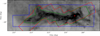 |
Fig. 1 Survey footprints of the image data. The blue outlines show the area covered by the J, H, and Ks filters, the green box shows the area covered by the four IRAC filters, and the red lines highlight the area observed in the MIPS 1 filter. The background image shows the dust emission from the Planck satellite at 545 GHz (Planck Collaboration 2020). |
2.2 Data extraction and preprocessing
To find distinct morphological families of YSOs, we created post-stamp cutouts from the mosaic images centered on the sky coordinates of the sources in the NEMESIS YSO catalog (Roquette et al. 2025). Since the main features we wished to identify are the morphological structures surrounding the central objects, we had to choose the size of the image stamps appropriately. This entailed weighting a larger stamp size to include jets and outflows that have already traveled farther from the source or are only visible at larger distances to the YSO against contamination from unrelated nearby sources and structures such as cloud emission from the surrounding ISM. This is very challenging in highly crowded areas such as the Orion nebula cluster (ONC). We finally converged toward a stamp size of 50 × 50 arcsec, which at a mean distance of 414 pc to the OSFC (Menten et al. 2007) corresponds to a square of approximately 20 000 × 20 000 au. Image stamps of this size contain the protostellar disk (size on the order of a few dozen to several hundred au; Tobin et al. 2020) and envelope (can reach a size of several thousand au; Heimsoth et al. 2022). They further partially cover jets and shocked material that emerges from the protostellar envelope, while keeping contaminating sources manageable.
For our training set, we extracted ≈ 10 000 image cutouts per filter. The total number of post-stamp image cutouts gained from each passband is given in Table A.1.
Downsampling the NIR images to a lower resolution has the benefit of shorter computation times when they are plugged into our machine-learning algorithm. As long as the new pixel scale stays below the seeing limit of the VISION survey, no spatial information is lost. Since the image resolution of VISION is limited by seeing which is 0.78″, 0.75″, and 0.8″ on average in the J, H, and Ks-bands, respectively (Meingast et al. 2016), we opted to resample the images to a resolution of 2 × 10⁻⁴ deg px−1, which equals 0.72″px−1.
To clean the images in the training set from image artifacts caused by saturated sources or sources that lie on the border of the image mosaic, we removed all images containing NaN values. In total, we removed 492, 252, and 257 sources from the sample in the J-, H-, and KS-band images, respectively. Table 1 gives a detailed overview on the absolute and relative numbers of removed sources with respect to the total number in the training set. The table also lists in parentheses the relative number of removed sources with respect to the number of sources in each class as determined by the αIR index (see Table 2).
Spitzer images, albeit diffraction limited, have a lower resolution because the aperture of the telescope is smaller and the pixel scale of the detectors is larger. The IRAC 1, 2, 3, and 4 passband images have an average point spread function FWHM of 1.66″, 1.72″, 1.88″, and 1.98″, respectively3. Furthermore, the MIPS 1 images have the lowest resolution, with an FWHM of 6″4.
For PINK to learn morphological prototypes, the YSO features, that is, structures directly related to the forming star, such as jets, outflows, and outflow cavities, must be directly visible in the input images. Without further processing, these features are not necessarily immediately apparent as they may be hidden in the high dynamic range of the images. Thus, it is paramount to find an optimal flux scaling that brings out these features and suppresses unrelated structures as best as possible.
To this end, we applied the stretching and normalization method developed by Lupton et al. (2004) to the image cutouts. In general, the Lupton method allows us to stretch three filters together so that the color relations between the three channels are preserved, but single-channel flux scaling is also possible. We opted to process each channel individually, especially because preliminary experiments with PINK had failed because the three-channel mode had introduced processing artifacts that were confused for true features of YSOs by the SOM. We experimented with other image preprocessing methods as well, but with limited success. It is very challenging to automatically process a large number of image cutouts containing different morphological structures. For a morphological analysis alone, our chosen preprocessing is sufficient, but for a future spectro-morphological classifier, the flux-scaling method should be revisited.
Number of images removed from the training sample.
YSO classes and corresponding spectral index ranges.
3 Method
In this section, we describe the standard classification scheme for YSOs we used as the classification baseline for the morphological analysis. More importantly, we show how we created morphological prototypes of YSOs using the PINK self-organizing map algorithm. Using Bayesian inference, we explore how different observational classes are linked to the morphological prototypes on the SOMs. This enables us to identify typical source morphologies associated with certain classes of YSOs.
3.1 Standard classification of YSOs
We first required homogeneously determined evolutionary classes for our YSO sample to link different YSO morphologies to an evolutionary stage. To do this, the classification scheme used by Großschedl et al. (2019), which is based on the observational classes first defined by Lada (1987), was adopted. This method uses the shape of the infrared SED to estimate the true evolutionary stage and assigns an observational class accordingly. We approximated the shape of the SED using the αIR index. To build a baseline of YSO classes for our training sample, we used nonlinear least-squares fitting to fit a power law in the range from 2 to 24 μm to the infrared SED. We used all available photometric data available in that wavelength range for the fit.
With αIR determined, we assigned the observational class of the YSO using the αIR-index ranges as reported by Großschedl et al. (2019). By this definition, we have five distinct YSO classes: Class 0/I protostars, flat-spectrum sources, Class II T-Tauri stars, Class III sources with a thin disk (anemic or debris disk), and diskless Class III pre-main-sequence or main-sequence stars. Table 2 lists the spectral index ranges reported by Großschedl et al. (2019). Sources with few data to compute the αIR index were not classified.
3.2 Self-organizing maps
The SOMs are artificial neural networks (Kohonen 1982) that are used to reduce the dimensionality of high-dimensional complex data (Kohonen 2001). In other words, an SOM provides a latent, low-dimensional, and discrete feature space that embeds the data, so that each data point from the input set can be characterized by its location and neighborhood in the latent space. We applied this method to a sample of NIR and MIR images (see Sect. 2.1) of YSOs to build a grid of artificial image prototypes representing observed YSO morphologies in our training sample. These images can be represented as a vector, where the vector dimension is equal to the number of pixels in the image. Thus, the general features of the high-dimensional data can be expressed through the coordinates of the low-dimensional latent space. In return, each location in the discrete latent space is equivalent to a high-dimensional image prototype, through which the embedding takes place based on the similarity of the prototype to the input images. In our case, where the input images showed many morphological features of YSOs, the SOM created a limited number of prototypes that showed us how many different YSO morphologies were observed in the training set. This enabled us to quantitatively analyze the YSO morphology without visually inspecting thousands of image cutouts one by one.
Moreover, an SOM is an unsupervised machine-learning technique that allows us to create the prototypes in a data-driven way without relying on a theoretical model calculation using radiative transfer codes such as those used by Robitaille et al. (2007). The following paragraphs provide an overview of how an SOM works, and we introduce the PINK algorithm (Polsterer et al. 2016) we used.
The algorithm PINK is an SOM that creates rotation- and flipping-invariant prototypes for images of astronomical objects. We used PINK to create a grid of exemplary images of YSOs that we then associated with their evolutionary stage via the αIR index. To create this image grid of the morphological prototypes of YSOs, we initialized a Cartesian grid of n × m neurons in a random state, that is, a noise image, and trained the SOM in an iterative process that can be roughly divided into five steps, as listed below
Draw a random element from the training sample.
Create copies at different rotation and flipping states (specific to PINK)
Find the best-matching unit (BMU).
Compute the weights for all neurons in the map.
Update the neurons in the map.
Optional: adapt the learning rate and neighborhood function. These steps are repeated until the SOM has settled. An SOM is considered settled either after the model has undergone a predefined number of epochs or when the change of the SOM over several epochs stays below a certain threshold and the network learns no new features (Kohonen 2001). To train our SOMs, we opted for a very simple training scheme.
Overview of the PINK training hyperparameters.
3.3 SOM training strategy and hyperparameters
For the best results, we fine-tuned the hyperparameters and divided the SOM training into two phases. We first populated the maps with a coarse version of possible morphologies by letting the algorithm run for 1 000 epochs, choosing a broad neighborhood function and a high learning rate. The main learning phase for the SOM ran for 15 000 epochs, but this time, with a narrow neighborhood function and a low learning rate. We give additional information of our choice of the hyperparameters in Appendix A. Table 3 gives a brief overview of these hyperparameters.
PINK can handle image rotation of up to 1°, that is, 360 possible rotations (angles of freedom) per image. To save computation time, however, we limited the number of possible rotations to 24 and 92 for the first and second phases of training, respectively. Choosing fewer rotations for the first phase decreases the computation time, but creates coarse prototypes. For smoother, more detailed neurons, we increased the number of rotations to 92 for the main training phase (see Sect. 4.1). The two training phases permit image-flipping during training.
Furthermore, we chose a Cartesian noncyclic boundary topology for our map with a size of 20 × 20 neurons (see Appendix A for further details of the chosen grid dimensions). In contrast to a cyclic boundary where the opposite edges and all corners of a square map connect, which results in a doughnutshaped topology, the corners and edges of the SOM provide a space into which distinct morphologies can retreat and cluster together. This helps the algorithm to better separate different morphologies.
The map size of the SOM controls the sensitivity of the map to differences in the morphology at a given abundance of expected morphological classes. For example, if 10% of the sources in the training sample exhibit morphologies other than point sources and the SOM size is limited to ten neurons, that is possible morphological prototypes, then we expect that nine neurons show prototypes for point sources and only one prototype for all species of extended sources. Similar findings were reported by Vantyghem et al. (2024, see chapter 9 therein), along with possible remedies to counter the effect of underrepresented morphologies.
In our case, the extended YSOs, those in the main formation stages that we investigated, make up roughly 10% of our training sample. To enable the SOM to also learn underrepresented morphologies, we chose to optimize the number of neurons in the SOM, as was also suggested by Vantyghem et al. (2024). An SOM-size of 20 × 20 neurons yielded the best results without overfitting the model, which would be the case if we had as many neurons as there are sources in our training sample, and it resulted in one prototype for approximately 25 sources.
Finally, we created heatmaps to compare and determine a relation between the YSO morphologies and the current standard classification, that is, the αIR index. We used a Bayesian approach to map the individual YSO images from our training sample to the SOM prototypes. This provided us with a statistically sound framework that took the estimated noise in each image into account when the observations were mapped to the SOM. The result was a probability distribution function on the SOM grid space for each filter.
4 Experiments
This section is dedicated to our experiments with PINK. We provide some details of our final training parameters and the filters we used to create the morphological prototypes. In addition, we show how we verified that the training of the maps was successful.
4.1 Training the maps
Because we trained the maps for each filter individually, it was not guaranteed that similar morphologies would be found in the same locations on the maps for each filter if they were initialized randomly. That is, the prototypes found in the top left corner of the map for the J band might not be the same as those found in the top left corner of the map for any other passband. To keep the maps comparable across filters, only the J-band SOM was initialized in a random state. The SOMs for the longer wavelengths were then initialized with the fully trained SOM from the previous wavelength, that is, the H-band SOM was initialized with the J-band SOM, and the Ks-band SOM was initialized with the H-band SOM. We thereby ensured that we were able to find similar prototypes in similar regions across the SOMs for each filter in general.
The maps were trained in two steps: an initial map-setting stage, and a main training stage. In the setting stage, we let the algorithm run for a 1000 epochs that were intended to populate the map with a first approximation of the different morphologies. At this stage, it is not too important to learn detailed YSO morphologies, and we therefore allowed a limited number of 24 rotations plus flipping of the images to speed up the computation. Furthermore, we set the neighborhood function in this stage to a Gaussian kernel with a standard deviation σ of 2.5 neurons. The learning rate was set to 0.1, which gave the input images a higher weight when the map was updated and also resulted in a faster population of the map.
The second stage allowed 92 rotations for each input image plus flipping, using a narrower kernel and a slower learning rate. The number of rotations here yielded a minimum rotation angle of 3.91°. Thus, at our chosen image size of 69 × 69 pixels, rotating the cutout by the minimum angle about the image center shifts the middle pixel at the outer boundary of the image by ≈2.5 pixels. Because this is the main learning stage for the SOM, we narrowed the width σ of the neighborhood function to one neuron in SOM coordinate space, dropped the learning rate to 0.05, and let the SOM train for 15 000 epochs.
4.2 Verifying the training
To verify that the maps were trained well, we used the PINK mapping functionality to create heatmaps for each image in the training sample. A heatmap contains the Euclidean distance between the input image and each neuron in the SOM. Thus, we were able to use the heatmaps to extract the coordinates of the BMU, that is, the neuron that is closest to the input image. We used the BMU coordinates to count how many images from the training sample mapped to each neuron in the SOM. Furthermore, we used a histogram of BMU distances for a second measure to assess the SOM training. In general, we required that two conditions were met. We first required that the mapped sources on the SOM were roughly uniform distributed, and we then required small Euclidean distances to the BMU for the majority of sources in the training sample.
For the first criterion in the J band, we would ideally expect that each neuron is the best-matching prototype for Nimgs J-band/Nprototypes sources, which results in ≈25 sources mapping to each neuron in this case. Figure 2 shows how the mapped J-band images are distributed over the SOM prototypes. The color map in the plot was chosen to facilitate detection of any deviations above and below the estimated number of mappings per neuron. Even though the source distribution on the map is not perfectly homogeneous, no disjunct overdensity island are found, which attract a majority of sources from the training sample. There are only two neurons (at [19,0] and [19,2]) in the bottom right corner of the map to which a significantly higher number of sources fit best.
This discrepancy can be explained by the composition of our data set. Based on the classical αIR index, we estimated that roughly 10% of all sources in the training sample exhibit interesting morphologies in the observed wavelengths, for instance, feedback cavities, jets, and outflows. The remainder of the sources appear as point sources that are hence overrepresented in the sample. Therefore, we cannot expect a perfectly uniform distribution of sources when mapping the images back onto the trained SOM.
To test the second criterion, we studied the distribution of BMU distances for each image in the sample. With a well-trained map, we expect that each image in the training sample is well represented by at least one neuron in the SOM. In reality, however, it is common that the neurons in the SOM are a good representation for the great majority of input images, but not for all. In terms of the BMU distances, this results in a BMU distance distribution that peaks at a very small Euclidean distance. A long tail of large distances shows the presence of outliers in the data that cannot be represented by the morphological prototypes learned by the SOM. Figure 3 shows the distribution of BMU distances for the J-band SOM. The distribution peaks at a distance of roughly 0.1 and steeply declines into a shallow tail of larger distances.
For the NIR maps, this fits our expectation from a well-trained SOM well, and we therefore conclude that the training of our NIR maps was successful. The maps created from images at the longer wavelengths may show different morphological prototypes, but the source distributions of back-mapped images onto the SOM show that the images are strongly concentrated along the edges and corners of the maps.
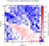 |
Fig. 2 Number of J-band image cutouts from the training sample mapping to the J-band SOM. The blue shades indicate regions on the SOM to which fewer than the expected number of sources are mapped, and the red shades highlight regions with more sources than expected after we mapped them back to the SOM. White indicates the expected number assuming a uniform distribution. |
5 Results
In the following, we present our results from training three maps, one for each filter for which we gathered the image cutouts. We created a grid of 400 morphological prototypes for each of the three filters. Furthermore, we analyzed the distribution of the αIR index and, hence, different observational classes over the SOMs. In this way, we were able to identify morphological prototypes representative of certain YSO classes in a quantitative and statistically robust way.
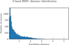 |
Fig. 3 J-band distribution of BMU distance of each image in the training sample. The successfully trained SOM features a distribution of BMU distances with a peak at very small distances and a tail of large distances representing outliers. |
5.1 Morphological prototypes of YSOs
Figure 4 shows the morphological prototypes we obtained from the J-band image cutouts. The SOMs showing the prototypes in the other NIR bands can be found in Appendix B. In the following, we explore the different morphologies that were learned through the PINK algorithm.
The large region on the left side that ranges from line 1 at the bottom to line 18 close to the top and extends from Cols. 1 to 10 is mostly populated by isolated point sources. The bottom right corner shows prototypes with extended emission from the surrounding ISM. In the J band, this extended emission can be attributed to the dust cloud, which scatters and reflects the light from the stars in the region. Some neurons only partially show extended emission, for example, the square of nine neurons centered around line 9, Col. 19, which might indicate that sources that map to these neurons are situated at the edges of the cloud. The map also shows prototypes that appear to have jet-like structures, for instance, in row 20, Cols. 1 through 6. Finally, we also observed two types of visual binaries that we called close and separated. The close binaries are those where the two points are connected; that is, their point spread functions touch, and the source looks elongated with or without a distinctive double peak. These close visual binaries can be found in the bottom left corner of the SOM. Separated binaries show a second isolated point source in the region surrounding the central point source, and the neurons show these prototypes in the top right corner of the map.
5.2 Observational class distribution of YSOs
To assess the distribution of the different observational classes in the SOM embedding space, we calculated for each image in our sample the prototype in the SOM that was most likely to represent the features contained in the input images. These probabilities enabled us to create heatmaps that highlight the observational classes that can be found in an area of the SOMs and, hence, give insight into whether the αIR index and the morphology of a YSO are linked.
The three rows in Fig. 5 show the probability density functions for each YSO class for each of the three SOMs trained with the images observed in one of the three NIR passbands, where the first, second, and third rows correspond to the J-, H-, and KS-band SOMs. Each of the five panels of each row show the most probable area in which the image of a specific class of YSO can be found. That is, each pixel in each heatmap represents the probability that the YSO prototype located at the same x and y coordinates in the SOM represents a YSO of the respective class. To help guide the eye when interpreting the probability distributions for each Class of YSO, we overplotted contours that enclose the area with 25%, 50%, and 75% of all YSOs of the respective class in each heatmap. The leftmost panel shows that Class 0/I YSOs are best represented by the morphological prototypes in the bottom right corner of the J-band SOM. This is also indicated by the contour lines that roughly enclose the bottom right 4 × 4 block of prototypes, which show that the morophologies of 50% of all Class 0/I YSOs are best represented by these prototypes. This can be interpreted as a strong correlation between the morphologies found in the bottom right prototypes and Class 0/I YSOs. The counter-conclusion is that Class 0/I YSOS and the morphologies found in the rest of the map are not correlated. The SOM has learned that this region contains images that exhibit significant emission from the surrounding medium and the central source is barely visible, if at all. This is consistent with what is expected in the J band because Class 0/I YSOs are hard to observe at this wavelength because the envelope of these deeply embedded proto-stars causes massive dust extinction.
Similar results were found for the flat-spectrum sources, which are shown in the second panel from the left of Figure 5. Even though the highest probability is again in the bottom right corner of the J- and H-band maps, the distribution also extends toward the top left corner, to the center of the SOM, so that the entire lower right quadrant contains possible morphologies in the SOM. There are additional high-probability morphologies in the top left corner, which are most evident in the H and Ks band (see Figures 5 middle and bottom rows), suggesting that the morphologies found in this area are significant for the flatspectrum sources. The prototypes in the top left corner show a central source in the middle of each neuron and a detached, triangle-shaped emission band that appears to be an outflow that starts rather narrowly and expands with distance from the central star.
The more evolved observational classes II, III with thin disk, and III no disk or MS star are harder to interpret because their probability distributions all appear to be very similar to each other. They generally avoid the regions in which the youngest (Class 0/I and flat-spectrum) sources were found (see Fig. 6), however, where the flat-spectrum sources act as an intermediate stage with higher levels of probability in the areas for the two YSO families, less and more evolved.
6 Discussion
We were able to identify certain regions in the SOM that are preferably inhabited by certain YSO classes. Our possible achievements with this method and the data at hand are limited, however. Thus, the following paragraphs discuss what we can learn from the trained SOMs and point out the current limitations. Finally, we also consider improvements of the results from this method in the future.
Based on the insights mentioned above in Sect. 5.2, it is possible to separate the earliest and latest stages of star formation. That is, based on morphology alone, we were able to distinguish Class 0/I proto-stars and flat-spectrum sources from older, more evolved Class II (classical T-Tauri) and Class III YSOs.
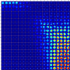 |
Fig. 4 J-band SOM prototypes. The numbers at the left and top edges indicate the coordinates in the latent space created by the self-organizing map algorithm, i.e., the coordinates of the neurons representing each prototype. |
6.1 Protostars
First, we consider the Class 0/I protostars. In the SOMs for the NIR filters (J, H, and Ks), they lie in the bottom right corner. In this region lie YSO prototypes with strong emission from the surrounding medium. In some cases, the prototypes also show central sources that are embedded in the medium. This agrees with what we expect for the least evolved, that is, for the youngest, YSOs in our sample. At this stage of star formation, a central source is deeply embedded in its protostellar envelope.
Although the central object actively accretes matter from its envelope through an accretion disk, which causes feedback mechanisms to expel a fraction of the infalling material back into the environment, these outflows have not had enough time to excavate much of the envelope. Thus, the jets and outflow cavities in close proximity to the source are hard to detect (if it is possible at all) in the NIR bands. The same is true for the central protostar itself.
Outflows driven by Class 0 YSOs were detected in the NIR and MIR bands, most notably, the Ks and IRAC2 bands, but they are often large structures that can reach parsec scales (see e.g., Bally & Devine 1994; Devine et al. 1997; Mader et al. 1999). We do not see them in our SOM prototypes because of the size of the image cutouts, which are about 20 000 × 20 000 au.
6.2 Flat-spectrum sources
Perhaps the most interesting results from our morphological analysis are the morphological prototypes associated with the flat-spectrum YSOs. The true nature of this class of YSOs is still heavily debated in the literature (see e.g., Crapsi et al. 2008; Dunham et al. 2015; Tobin et al. 2020). Common theories assume that this type of YSO represents an intermediate evolutionary stage between protostars and T-Tauri stars (Greene et al. 1994; Spezzi et al. 2011; Heiderman & Evans II 2015; Furlan et al. 2016), or that the flat spectrum is not a result of a distinct intermediate stage, but rather an effect of the physical orientation of the YSO with respect to the observer (Whitney et al. 2003b,a; Robitaille et al. 2006; Crapsi et al. 2008).
The most prominent characteristic of a flat-spectrum source is the flat slope of their infrared SED (αIR ≈ 0), which is eponymous to this class of YSO. The most common interpretations of the flat slope are that the central source contributes significantly, but the accretion disk and envelope contribute as well. Hence, the superposition of SEDs from the individual components results in the flat shape of the overall SED of the source. Furthermore, this class of YSO shows solid evidence of highly active accretion and feedback processes (Spezzi et al. 2011). Moreover, Heiderman & Evans II (2015) also argued in favor of an intermediate stage because they detected dense gas in close proximity to the central source of flat-spectrum YSOs that also contributes to the flat shape of the SED.
The prototypes associated with this class of YSO are split between sources that appear to be embedded in their surrounding environment and sources that show locally confined emission that goes in line with shocked material impacted by jets (see the second panel in each row of Figure 5). The YSO class probability distributions show that the flat-spectrum sources with outflow structures are most prominently present in the H- and Ks-band observations. This can be explained by strong line emission of molecular hydrogen (H2 at λ = 2.12 μm), which is excited when the jet rams the cloud surrounding these protostars (Ray & Ferreira 2021). Moreover, jets from YSOs commonly show forbidden iron lines ([Fe II] at λ = 1.64 μm) that can be detected in H-band observations (Reipurth & Bally 2001). This agrees well with our results, in which the areas of the SOMs show a high probability for flat-spectrum sources in the areas that are populated by prototypes with outflow signatures. Moreover, the splitting of flat-spectrum sources between two different morphologies, those with outflows and jets and those with embedded point sources, corroborates the results of Habel et al. (2021), who reported that flat-spectrum sources appear either as point sources or as irregular by their categorization.
Since the H2 and [Fe II] emission traces different components of the outflows (see e.g., Dionatos et al. 2018, 2020; Melnikov et al. 2023), we would expect this to be reflected in the observations of the YSOs and assumed that this is also learned by the SOM. The prototypes in the top left corner of the H and Ks band SOMs (those with jet structures) indeed appear to be somewhat narrower in the H band (sensitive to the [Fe II] line at λ = 1.64 μm) than they are in the Ks band (sensitive to the H2 line at λ = 2.12 μm).
The J and H band filter SOMs show a lower probability for jets. This might be explained by extinction effects in the shorter wavelengths. Reipurth & Bally (2001) reported additional bright lines of [Fe II] in the J and H band filters, but these lines are often difficult to detect as they are predisposed to extinction in the surrounding ISM. Atomic hydrogen lines in the NIR (Paβ and Brγ) were also observed and connected with YSO jets, but these lines are only observed in a small fraction of YSO outflows (Caratti o Garatti et al. 2015).
Moreover, Caratti o Garatti et al. (2015) pointed out that extinction effects often introduce an additional constraint to the detection of atomic jet tracers in the receding lobe of a bipolar outflow. In addition to this, Caratti o Garatti et al. (2015) also theorized that asymmetric matter distribution in a YSO envelope or source multiplicity can prohibit bipolar outflows altogether. This might explain why our prototypes primarily show unipolar outflow structures.
With this in mind, we would like to note that based on the morphology of the sources alone, we cannot give new insights into the nature of the flat-spectrum YSOs. Through our quantitative study of several thousand sources using unsupervised machine-learning, however, we see that YSO outflows have a high probability to be detected in the Ks-band observations of flat-spectrum sources, even more prominently than for the Class 0/I protostars. The lack of jet signatures found by the SOM for the youngest protostars can be attributed to the high extinction in the protostellar envelope, which effectively cloaks these outflow structures from our sight. On the other hand, it is possible that for stage I YSOs with visible outflows at low inclinations, that is, viewed down into the narrow feedback cavity of the envelope, the source might have been misclassified as a flat-spectrum source.
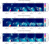 |
Fig. 5 Probability density function for each observational class in the J, H, and Ks band. These maps highlight the regions on the SOM in which the probability of finding a specific class of YSO is highest. The five panels from left to right show the probabilities per neuron for each class, starting with the youngest on the left and ending with the oldest, most evolved class to the right. The contours in each panel enclose the area within which 25%, 50%, and 75% of all YSOs of a given class are located within the map. |
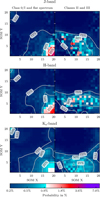 |
Fig. 6 Similar to Fig. 5. Probability density function for YSOs grouped into Class 0/I and flat spectrum sources and into Class II and III YSOs or MS stars. |
6.3 Class II and III YSOs
Finally, we are unable to separate the more evolved sources, that is, the Class II T-Tauri stars from the Class III pre-main-sequence stars. These objects have already consumed their protostellar envelopes, and what remains are at first thick, and as they evolve further, increasingly thinner disks as planets form. This further depletes the dust and gas in the disk. In addition, stellar winds blow the remaining gas away. Thus, the images of these systems predominantly show point sources. This directly results in a degenerate morphology that cannot be classified without further information, such as flux ratios from different filters or spectroscopic data. As a consequence, PINK is not able to learn any differences between these classes from the data available to us.
6.4 Limitations
Some limitations of using SOMs for morphological classification have already been mentioned in the sections above. We summarize these limitations and caveats below.
First to mention is the number and demography of sources in the training sample. From the 27 879 literature YSO candidates (Roquette et al. 2025), only about one-third (10 355) are observed by the VISION survey. In general, SOMs are trained on training sets that are larger by at least one to two orders of magnitude. To compensate for this, we had to extend the number of training epochs to arrive at maps that were well trained. One possible path to explore in a future paper would be to train PINK on images obtained from theoretical models (see, e.g., Whitney & Hartmann (1992, 1993) or Robitaille (2011), which would create a large enough dataset of synthetic YSO images.
A more serious caveat is the composition of morphologies found in the training sample. Out of the 10 355 sources, we were able to calculate αIR indices for ≈8 355 objects. Interesting morphologies such as jets, outflow cavities, and shocked material, which are mainly a feature of YSOs in their earliest stages of evolution, are rarest. Hence, these morphologies are largely underrepresented in the training sample. Based on the number of sources for which we derived an observational class (≈8355), Class 0/I (723) and flat-spectrum sources (628) only account for roughly 20% of the sources. When the literature estimates for the fraction of the youngest YSOs from Großschedl et al. (2019), for example, are taken into account, this fraction lies at 12.5%, which is even lower than the 20% given above.
We wish the SOM to learn a large variety of different morphologies, for instance, outflow cavities with different opening angles seen from various inclination angles, with or without jets, bipolar or monopolar. This becomes an immense challenge when they are rare compared to other dominant morphologies, such as point sources. One way to counter this issue would be to remove all point sources, which could be easily done using the SOM by excluding all sources that map back onto the prototypes representing a point source. This was no option here, however, because this would shrink the size of our training set too much for it to still be a viable sample.
Another limitation we found is the resolution of the observations. To distinguish different morphologies, we required the defining features of these morphologies to be spatially resolved. With protostellar disk sizes ranging from a few dozen to several hundred au, VISTA/VIRCAM (with a pixel scale of 1/3″ per px ;0.72″ per px after resampling, which at the distance of Orion equates to ≈150 au/px (≈300 au/px after resampling) is powerful enough to potentially resolve the protostellar disks and outflows, the latter of which are typically significantly larger than the disks. Unfortunately, the resolution of the MIR images from Spitzer was not high enough for us to come to a satisfying conclusion.
While training our SOMs, we also identified crowding as a limiting factor that affects the performance of our morphology analysis, especially in the ONC and its immediate neighborhood. To a certain extent, crowding can be managed by choosing an appropriate size of the image cutouts. Ideally, we wish to have only the YSO and its outflows in the image. To include the entire system, especially with large-scale outflows, a larger stamp size would be better. With increasing image dimensions, more unrelated contaminating sources will be included in the image, however. Hence, the image dimensions must be carefully weighted between a larger size to encompass much of the outflows and a smaller size to limit contaminating sources that can confuse the SOM algorithm.
Unfortunately, the image stamp size chosen in our case cannot exclude all contaminating sources from the cutouts. We found that slightly fewer than 60% contain at least two sources that are listed in the NEMESIS catalog (see Sect. 2.1). In absolute numbers, this amounts to 5675, 5874, and 5848 for the J, H, and KS band image cutouts, respectively. Out of the multiple source images, the ratio of cutouts with only two and those with more than two YSOs is approximately 40% to 60%. The SOMs we trained do show prototypes for binary sources, but we did not observe any prototypes containing more than two sources. Even though PINK is a rotation- (about the center of the image) and flipping- (along all axes running through the image center) invariant implementation of an SOM, it is not invariant to the number of sources or their spatial arrangement inside the image cutout.
To understand how PINK handles cases of multiple sources, we considered two general cases. First, an image containing two distinct sources. Since the image cutouts are centered on the YSO coordinates from the input catalog, one source is always in the center, and the second source will be somewhere off center. When PINK determines the best-matching unit, it creates copies of the original image at various rotation angles and flipping states. For the SOM update, the algorithm only keeps the copy that fits the BMU on the SOM best. The only parameter PINK cannot compensate for in this case is the separation between the two sources, and therefore, several similar prototypes show binary sources with different separation. The second case considers an image with more than two visible sources in the image. Here, we have two parameters per off-center source that are not marginalized by PINK, the separation and the direction in which the off-center source lies in the image. As a result, these images are similar to noise because the spatial distribution of the sources, with exception of the source at the image center, is practically random. These images are therefore treated by PINK as morphological outliers whose morphology is not learned, that is, they not represented in any of the prototypes. This is a double-bladed sword. On the one hand, it may be beneficial that PINK somewhat ignores images that are contaminated by crowding. On the other hand, however, there is no guarantee that PINK associates a potential morphological distinctiveness of the source at the image center with a prototype that represents this morphology because of the surrounding contaminating sources in the input image.
7 Conclusion
Using a rotation- and flipping-invariant self-organizing map algorithm, we created a grid of morphological prototypes of young stellar objects for eight NIR and MIR bands. This allowed us to explore stellar evolution in the earliest stages of the life cycle of a star. We found that the best results were produced with the images obtained from the NIR survey VISION.
This study in the Orion A molecular cloud is a preparatory work for a future spectro-morphological classification scheme for YSOs. The lessons learned in this paper will directly influence future improvements to the method with the aim to use morphological information extracted with PINK (either from observed or synthetic images) and combine them with spectral information, for instance, from SEDs and spectra, to develop an improved and more reliable classification for YSOs.
In contrast to an analysis that is driven by a model hypothesis, we showed that in a data-driven quantitative analysis of different YSO morphologies, unsupervised self-organizing maps are an effective tool for investigating early stellar evolution when the sample size is large and the resolution of the images in the training set is high enough. We successfully separated less evolved YSOs (i.e., Class 0/I protostars and flat-spectrum sources) from the more evolved Class II and III YSOs. Moreover, we found that flat-spectrum sources show a high probability for prototypes that represent embedded jet-launching sources. This agrees with the hypothesis that flat-spectrum sources are an intermediate stage between Class 0/I and Class II, as suggested in the literature.
Moreover, along with the typical morphologies we expect from young protostars, we found that PINK has also learned the morphology of close and separated double-point sources. Although we did not investigate these morphologies closely, PINK might be used to identify and analyze true and visual binaries in the sample. Upon visual inspection of the VISION image data during our analysis, we further noted a large number of resolved galaxies. Our sample of YSOs in Orion contains a small number of galaxies, but not enough to impact our YSO morphology prototypes noticeably. Nevertheless, PINK (if it were trained on VISION NIR images of galaxies) might prove useful to researchers who focus on galaxies.
Acknowledgements
This work is part of the NEMESIS project which has received funding from the European Union’s Horizon 2020 research and innovation program under grant number 101004141. G.M. acknowledges support from the János Bolyai Research Scholarship of the Hungarian Academy of Sciences. This research was supported by the International Space Science Institute (ISSI) in Bern, through ISSI International Team project 521 selected in 2021, Revisiting Star Formation in the Era of Big Data (https://teams.issibern.ch/starformation/). We would also like to thank the anonymous referee for their valuable input from which this paper has greatly benefited.
References
- Aly, S., Tsuruta, N., & Taniguchi, R.-I. 2008, Artif. Life Robot., 13, 298 [Google Scholar]
- Andre, P., Ward-Thompson, D., & Barsony, M. 1993, ApJ, 406, 122 [NASA ADS] [CrossRef] [Google Scholar]
- Bally, J., & Devine, D. 1994, Astrophys. J., 428, L65 [Google Scholar]
- Caratti o Garatti, A., Stecklum, B., Linz, H., Garcia Lopez, R., & Sanna, A. 2015, Astron. Astrophys., 573, A82 [Google Scholar]
- Chen, H., Myers, P. C., Ladd, E. F., & Wood, D. O. S. 1995, ApJ, 445, 377 [NASA ADS] [CrossRef] [Google Scholar]
- Crapsi, A., van Dishoeck, E. F., Hogerheijde, M. R., Pontoppidan, K. M., & Dullemond, C. P. 2008, Astron. Astrophys., 486, 245 [Google Scholar]
- Devine, D., Reipurth, B., & Bally, J. 1997, in Herbig-Haro Flows and the Birth of Stars, 182, 91 [Google Scholar]
- Dionatos, O., Ray, T., & Güdel, M. 2018, Astron. Astrophys., 616, A84 [Google Scholar]
- Dionatos, O., Kristensen, Lars. E., Tafalla, M., Güdel, M., & Persson, M. 2020, Astron. Astrophys., 641, A36 [Google Scholar]
- Drakopoulos, G., Giannoukou, I., Mylonas, P., & Sioutas, S. 2020, in Database and Expert Systems Applications, 12392, eds. S. Hartmann, J. Küng, G. Kotsis, A. M. Tjoa, & I. Khalil (Cham: Springer International Publishing), 195 [Google Scholar]
- Drążkowska, J., Bitsch, B., Lambrechts, M., et al. 2023, in Astronomical Society of the Pacific Conference Series, 534, Protostars and Planets VII, 1st edn. (San Francisco: Astronomical Society of the Pacific), 717 [Google Scholar]
- Dunham, M. M., Allen, L. E., Evans, II, N. J., et al. 2015, Astrophys. J. Suppl. Ser., 220, 11 [Google Scholar]
- Evans, N. J., Dunham, M. M., Jørgensen, J. K., et al. 2009, ApJS, 181, 321 [NASA ADS] [CrossRef] [Google Scholar]
- Furlan, E., Fischer, W. J., Ali, B., et al. 2016, Astrophys. J. Suppl. Ser., 224, 5 [Google Scholar]
- Greene, T. P., & Lada, C. J. 2002, Astron. J., 124, 2185 [Google Scholar]
- Greene, T. P., Wilking, B. A., Andre, P., Young, E. T., & Lada, C. J. 1994, Astrophys. J., 434, 614 [Google Scholar]
- Großschedl, J. E., Alves, J., Teixeira, P. S., et al. 2019, A&A, 622, A149 [NASA ADS] [CrossRef] [EDP Sciences] [Google Scholar]
- Gutermuth, R. A., Megeath, S. T., Myers, P. C., et al. 2009, ApJS, 184, 18 [Google Scholar]
- Habel, N. M., Megeath, S. T., Booker, J. J., et al. 2021, Astrophys. J., 911, 153 [Google Scholar]
- Heiderman, A., & Evans II, N. J. 2015, ApJ, 806, 231 [NASA ADS] [CrossRef] [Google Scholar]
- Heimsoth, D. J., Stephens, I. W., Arce, H. G., et al. 2022, Astrophys. J., 927, 88 [Google Scholar]
- Kenyon, S. J., Whitney, B. A., Gomez, M., & Hartmann, L. 1993, ApJ, 414, 773 [Google Scholar]
- Koenig, X. P., & Leisawitz, D. T. 2014, ApJ, 791, 131 [Google Scholar]
- Kohonen, T. 1982, Biol. Cybernet., 43, 59 [CrossRef] [Google Scholar]
- Kohonen, T. 2001, Springer Series in Information Sciences, Vol. 30, SelfOrganizing Maps, 3rd edn. (Berlin, Heidelberg: Springer-Verlag Berlin Heidelberg) [Google Scholar]
- Lada, C. J. 1987, Symp. Int. Astron. Union, 115, 1 [Google Scholar]
- Lada, C. J., & Wilking, B. A. 1984, ApJ, 287, 610 [NASA ADS] [CrossRef] [Google Scholar]
- Lada, C. J., & Lada, E. A. 2003, Annu. Rev. Astron. Astrophys., 41, 57 [Google Scholar]
- Lupton, R., Blanton, M. R., Fekete, G., et al. 2004, Publ. Astron. Soc. Pac., 116, 133 [Google Scholar]
- Mader, S. L., Zealey, W. J., Parker, Q. A., & Masheder, M. R. W. 1999, Mon. Not. R. Astron. Soc., 310, 331 [Google Scholar]
- McClure, M. K., Furlan, E., Manoj, P., et al. 2010, ApJS, 188, 75 [NASA ADS] [CrossRef] [Google Scholar]
- Megeath, S. T., Gutermuth, R., Muzerolle, J., et al. 2012, AJ, 144, 192 [NASA ADS] [CrossRef] [Google Scholar]
- Meingast, S., Alves, J., Mardones, D., et al. 2016, Astron. Astrophys., 587, A153 [Google Scholar]
- Melnikov, S., Boley, P. A., Nikonova, N. S., et al. 2023, A&A, 673, A156 [NASA ADS] [CrossRef] [EDP Sciences] [Google Scholar]
- Menten, K. M., Reid, M. J., Forbrich, J., & Brunthaler, A. 2007, Astron. Astrophys., 474, 515 [Google Scholar]
- Morbidelli, A., & Raymond, S. N. 2016, JGR Planets, 121, 1962 [Google Scholar]
- Myers, P. C., & Ladd, E. F. 1993, ApJ, 413, L47 [NASA ADS] [CrossRef] [Google Scholar]
- Padgett, D. L., Brandner, W., Stapelfeldt, K. R., et al. 1999, Astron. J., 117, 1490 [Google Scholar]
- Palla, F. 1996, in Lecture Notes in Physics, 465, Disks and Outflows Around Young Stars: Proceedings of a Conference Held at Heidelberg, Germany, 6-9 September 1994, eds. S. Beckwith, J. Staude, A. Quetz, & A. Natta (Berlin, Heidelberg: Springer), 143 [Google Scholar]
- Planck Collaboration I. 2020, Astron. Astrophys., 641, A1 [CrossRef] [EDP Sciences] [Google Scholar]
- Polsterer, K. L., Gieseke, F., Igel, C., Doser, B., & Gianniotis, N. 2016, in 24th Eur. Symp. Artif. Neural Netw. Comput. Intell. Mach. Learn. ESANN 2016 Bruges Belg April 27-28-29 2016 Proc., Louvain-la-Neuve, Belgique, 405 [Google Scholar]
- Ray, T., & Ferreira, J. 2021, New Astron. Rev., 93, 101615 [CrossRef] [Google Scholar]
- Rebull, L. M., Padgett, D. L., McCabe, C.-E., et al. 2010, ApJS, 186, 259 [NASA ADS] [CrossRef] [Google Scholar]
- Reipurth, B., & Bally, J. 2001, Annu. Rev. Astron. Astrophys., 39, 403 [Google Scholar]
- Robitaille, T. P. 2011, A&A, 536, A79 [NASA ADS] [CrossRef] [EDP Sciences] [Google Scholar]
- Robitaille, T. P., Whitney, B. A., Indebetouw, R., Wood, K., & Denzmore, P. 2006, Astrophys. J. Suppl. S, 167, 256 [Google Scholar]
- Robitaille, T. P., Whitney, B. A., Indebetouw, R., & Wood, K. 2007, Astrophys. J. Suppl. S, 169, 328 [Google Scholar]
- Roquette, J., Audard, M., Hernandez, D., et al. 2025, The NEMESIS Catalogue of Young Stellar Objects for the Orion Star Formation Complex. I. General Description of Data Curation [Google Scholar]
- Sheehan, P. D., Tobin, J. J., Looney, L. W., & Megeath, S. T. 2022, ApJ, 929, 76 [NASA ADS] [CrossRef] [Google Scholar]
- Shu, F. H., Adams, F. C., & Lizano, S. 1987, Annu. Rev. Astron. Astrophys., 25, 23 [CrossRef] [Google Scholar]
- Spezzi, L., Vernazza, P., Merín, B., et al. 2011, Astrophys. J., 730, 65 [Google Scholar]
- Terebey, S., Shu, F. H., & Cassen, P. 1984, Astrophys. J., 286, 529 [Google Scholar]
- Tobin, J. J., Sheehan, P. D., Megeath, S. T., et al. 2020, Astrophys. J., 890, 130 [Google Scholar]
- Vantyghem, A., Galvin, T., Sebastian, B., et al. 2024, Astron. Comput., 47, 100824 [Google Scholar]
- Whitney, B. A., & Hartmann, L. 1992, Astrophys. J., 395, 529 [Google Scholar]
- Whitney, B. A., & Hartmann, L. 1993, Astrophys. J., 402, 605 [Google Scholar]
- Whitney, B. A., Wood, K., Bjorkman, J. E., & Cohen, M. 2003a, ApJ, 598, 1079 [CrossRef] [Google Scholar]
- Whitney, B. A., Wood, K., Bjorkman, J. E., & Wolff, M. J. 2003b, ApJ, 591, 1049 [Google Scholar]
- Williams, J. P., & Cieza, L. A. 2011, Annu. Rev. Astron. Astrophys., 49, 67 [Google Scholar]
We received fully reduced mosaics from S. Meingast through private communication.
IRAC Instrument Handbook (https://irsa.ipac.caltech.edu/data/SPITZER/docs/irac/iracinstrumenthandbook/5/) accessed in November 2024.
MIPS Instrument Handbook (https://irsa.ipac.caltech.edu/data/SPITZER/docs/mips/mipsinstrumenthandbook/3/) accessed in November 2024.
Appendix A PINK - training
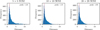 |
Fig. A.1 BMU distance histograms for SOM sizes of 5 × 5, 10 × 10, and 20 × 20 neurons. These histograms show the distribution of Euclidean distances between a YSO image and its corresponding best-matching unit for all source images in the training sample. From left to right, the panels show the distribution of BMU distances for increasing SOM sizes. The red vertical line indicates the position of the peak of the distance distribution. |
Similarity metric. To find the BMU, we have to define a measure of similarity (i.e., a distance measure) to compare the input data to the SOM output. Depending on the data, different distance metrics have been suggested (Kohonen 2001); Among them, the Euclidean distance (L2 - norm) is commonly used, but it has been suggested that other metrics may be better suitable in some cases (see e.g., Aly et al. 2008; Drakopoulos et al. 2020).
However, we will rely on simple Euclidean distance, as it already yields good results for our first attempt at determining morphological prototypes. Moreover, a detailed analysis of which similarity metric is best suited for YSO morphologies lies beyond the scope of this paper.
Map size:. Determining the best size for the SOM, i.e., the number of neurons, is essential as the SOM size determines the number of morphological prototypes. A first estimate for the number of neurons is to use the square root of the number of sources in the input data set  . However, the set of YSO images we retrieved is dominated by a large number of point sources. A rough estimate of the ratio between images showing point sources and images showing more complex YSOs is roughly 5%. This is an issue because these 5% contain the most interesting morphologies, but the map does not have enough space to represent them properly.
For example, in a training set of approximately 10 000 sources and an SOM size of  neurons, each neuron should become a best-matching prototype for 100 sources in the training set. When only 5% of the training set contains interesting morphologies beyond point sources, there are 5 neurons in the SOM representing all of these morphologies. There are several solutions to this under-representation of interesting morphologies. One is to increase the number of neurons in the SOM.
We can estimate the optimal size of the SOM by computing the pixel-wise Euclidean distance between each source in the training set and its best matching unit (BMU) in the SOM. If all morphologies are well represented in the SOM, the majority of distances to the BMUs are small. On the other hand, if a large number of diverse morphologies have the same BMUs, the distances to the BMU will increase. Thus, the histogram of BMU distances (see Figure A.1) can be used to measure the optimal SOM size.
Number of image cutouts per filter.
To determine the optimal SOM size, we aim for a narrow distribution, meaning that the majority of images in the training sample have a well-fitting best-matching unit generated by the SOM. Outliers, which are sources that are not well represented by any of the morphological prototypes in the sOM, will have large distances compared to the majority of sources, located to the far right side of the histogram. Optimally, the tail to the far right of the distance distributions in Figure A.1 vanishes when approaching the optimal SOM size. At the same time, the peak of the distribution should move to the left as the bulk of the sources is better represented by the SOM prototypes. In Figure A.1, we compare the three different SOM sizes; the left panel shows the distance distribution for a 5 × 5 grid, the middle panel for a 10 × 10, and the tight panel for a 20 × 20 grid.
We settled for an SOM size of 20 × 20 neurons, as the distance distribution peaks at 1.03, which is the lowest of the three map sizes (1.24 for the 5 × 5, and 1.10 for the 10 × 10 maps). Moreover, the histogram of the 20 × 20 grid has a short tail to the right, i.e. few outliers not well represented by the prototypes. Thus, we deemed the 20 × 20 map is best suited for our experiments.
Increasing the SOM size further bears the risk of overfitting the model since a larger number of neurons means that there are fewer sources from the training sample map for each prototype. In the extreme case of having just as many neurons, or more, as there are sources in the training set, we would expect to find each input image reflected in exactly one neuron of the map, hence overfitting the model. Yet, there may be some information gained from such an SOM, as it still should group similar sources in similar regions of the map.
Number of image cutouts:. The total number of image cutouts is slightly different in the individual passbands. This is explained by various differing observation footprints and detector sensitivities. The final number of cutouts per filter is shown in Table A.1.
Appendix B PINK - Self Organizing Maps
Full-size SOMs for the remaining filters not shown in the main text: H and Ks passbands are shown in Figures B.1 and B.2.
All Tables
All Figures
|
Fig. 1 Survey footprints of the image data. The blue outlines show the area covered by the J, H, and Ks filters, the green box shows the area covered by the four IRAC filters, and the red lines highlight the area observed in the MIPS 1 filter. The background image shows the dust emission from the Planck satellite at 545 GHz (Planck Collaboration 2020). |
| In the text | |
|
Fig. 2 Number of J-band image cutouts from the training sample mapping to the J-band SOM. The blue shades indicate regions on the SOM to which fewer than the expected number of sources are mapped, and the red shades highlight regions with more sources than expected after we mapped them back to the SOM. White indicates the expected number assuming a uniform distribution. |
| In the text | |
|
Fig. 3 J-band distribution of BMU distance of each image in the training sample. The successfully trained SOM features a distribution of BMU distances with a peak at very small distances and a tail of large distances representing outliers. |
| In the text | |
|
Fig. 4 J-band SOM prototypes. The numbers at the left and top edges indicate the coordinates in the latent space created by the self-organizing map algorithm, i.e., the coordinates of the neurons representing each prototype. |
| In the text | |
|
Fig. 5 Probability density function for each observational class in the J, H, and Ks band. These maps highlight the regions on the SOM in which the probability of finding a specific class of YSO is highest. The five panels from left to right show the probabilities per neuron for each class, starting with the youngest on the left and ending with the oldest, most evolved class to the right. The contours in each panel enclose the area within which 25%, 50%, and 75% of all YSOs of a given class are located within the map. |
| In the text | |
|
Fig. 6 Similar to Fig. 5. Probability density function for YSOs grouped into Class 0/I and flat spectrum sources and into Class II and III YSOs or MS stars. |
| In the text | |
|
Fig. A.1 BMU distance histograms for SOM sizes of 5 × 5, 10 × 10, and 20 × 20 neurons. These histograms show the distribution of Euclidean distances between a YSO image and its corresponding best-matching unit for all source images in the training sample. From left to right, the panels show the distribution of BMU distances for increasing SOM sizes. The red vertical line indicates the position of the peak of the distance distribution. |
| In the text | |
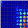 |
Fig. B.1 H-band SOM prototypes. Similar to Figure 4. |
| In the text | |
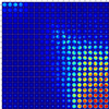 |
Fig. B.2 Ks-band SOM prototypes. Similar to Figure 4. |
| In the text | |
Current usage metrics show cumulative count of Article Views (full-text article views including HTML views, PDF and ePub downloads, according to the available data) and Abstracts Views on Vision4Press platform.
Data correspond to usage on the plateform after 2015. The current usage metrics is available 48-96 hours after online publication and is updated daily on week days.
Initial download of the metrics may take a while.