| Issue |
A&A
Volume 707, March 2026
|
|
|---|---|---|
| Article Number | A118 | |
| Number of page(s) | 15 | |
| Section | Interstellar and circumstellar matter | |
| DOI | https://doi.org/10.1051/0004-6361/202554309 | |
| Published online | 10 March 2026 | |
Shaping the interstellar medium through expanding H I shells
1
Instituto de Astronomía y Física del Espacio,
Ciudad Universitaria – Pabellón 2, Intendente Güiraldes 2160 (C1428EGA),
Ciudad Autónoma de Buenos Aires,
Argentina
2
Facultad de Ciencias Astronómicas y Geofísicas, Universidad Nacional de La Plata, Paseo del Bosque s/n,
1900
La Plata,
Argentina
3
Instituto de Astrofísica de La Plata (CONICET-UNLP), Paseo del Bosque s/n,
La Plata
B1900FWA,
Argentina
★ Corresponding author: This email address is being protected from spambots. You need JavaScript enabled to view it.
Received:
27
February
2025
Accepted:
24
December
2025
Abstract
Aims. The goal of this study is to analyse a set of four H I shells and their potential role in triggering star formation.
Methods. We analysed the H I 21-cm line and far-infrared emission distributions to characterize the four shells. To investigate star formation associated with these shells, we identified massive OB-type star candidates using Gaia data and a spectrophotometric method.
Results. The H I characterisation of the four shells reveals that they are expanding structures, with expansion velocities ranging from 6 to 9 km s−1 and kinetic energies between 2.5 × 1048 and 8.4 × 1048 erg. Some of the shells appear to be in collision with each other. The analysis of the IR emission reveals the presence of 28 H II regions seen projected into the borders of the H I shells, some of them located at the interfaces of two shells. The spectrophotometric analysis used to identify ionising star candidates in these regions indicates a distance of 2.7 ± 0.5 kpc for 27 of the H II regions. Since their radio recombination line (RRL) velocities are consistent with the systemic velocities of the H I shells, we can infer that the shells are located at the same distance.
Conclusions. The distribution of 27 H II regions along the borders of four H I shells is consistent with a scenario in which the massive stars responsible for their ionisation may have formed as a consequence of the shells’ expansion and, in some cases, their collision.
Key words: stars: formation / ISM: bubbles / HII regions / ISM: kinematics and dynamics
PhD Fellow of CONICET, Argentina.
© The Authors 2026
 Open Access article, published by EDP Sciences, under the terms of the Creative Commons Attribution License (https://creativecommons.org/licenses/by/4.0), which permits unrestricted use, distribution, and reproduction in any medium, provided the original work is properly cited.
This article is published in open access under the Subscribe to Open model. This email address is being protected from spambots. You need JavaScript enabled to view it. to support open access publication.
1 Introduction
Neutral hydrogen (H I) shells are structures that have been recognised as essential features in our Galactic interstellar medium (ISM). These structures, often shaped like shells or arc-like formations, hold crucial information about the underlying physical processes responsible for their formation and their potential impact on star formation within their vicinity.
The H I shells and supershells, large structures with diameters exceeding 200 pc, have been detected and catalogued using different H I databases and identification techniques (Heiles 1979; McClure-Griffiths et al. 2002; Ehlerová & Palouš 2005, 2013; Suad et al. 2014).
The origin of the supershells is still a subject of debate. Several mechanisms have been proposed that could have possibly led to their formation, including the cumulative effects of stellar winds and/or supernova explosions (McCray & Kafatos 1987; Tenorio-Tagle & Bodenheimer 1988; Kim & Ostriker 2015; Suad et al. 2019), as well as the interaction with high-velocity clouds (HVCs) (Tenorio-Tagle 1981). Assessing the kinetic energies of the shells and considering their dynamic ages is a way to constrain the most likely processes responsible for their creation. In this context, Suad et al. (2019) calculated the kinetic energies of the structures catalogued by Suad et al. (2014), shedding light on the ongoing debate regarding their origin. The calculated energy values ranged from 1 ×1047 to 3.4 ×1051 erg, falling within a range that aligns with the potential influence of stellar winds and/or supernova explosions associated with OB associations. These energy levels were estimated by assuming a 20% efficiency in converting the mechanical energy of stellar winds into the kinetic energy of Galactic shells, as suggested by Weaver et al. (1977).
The expansion of Galactic shells into the ISM has significant implications for star formation processes. It creates cool and dense regions with high column density on vast spatial scales (Dawson et al. 2011a, 2013; Dawson 2013), which can potentially become gravitationally unstable and trigger the formation of new stars, particularly along the periphery of the H I structures (McCray & Kafatos 1987; Oey et al. 2005; Zucker et al. 2022; O’Neill et al. 2024).
The collision of expanding H I shells is another well-known mechanism of triggered star formation, as it was reproduced in numerical and analytical models by different authors (Chernin et al. 1995; Ntormousi et al. 2011). Inutsuka et al. (2015) proposed a ‘bubble-dominated’ model for molecular cloud formation, suggesting a multi-generational process in which giant molecular clouds (GMCs), capable of hosting star formation, form in overlapping regions of shells from cold H I. High-resolution magneto-hydrodynamical simulations reveal that magnetic pressure resists cloud contraction (Inoue & Inutsuka 2008, 2009; Ntormousi et al. 2017), indicating that dense clouds with particle densities greater than 103 cm−3 require repeated episodes of supersonic compression (Inutsuka et al. 2015). As a result, the interfaces of the colliding H I shells may provide ideal conditions for GMC formation. Although shock waves from colliding H I shells are considered a potential mechanism for molecular cloud formation and subsequent star formation, only a few cases have been documented in our Galaxy, (e.g. Dawson et al. 2015; Gaczkowski et al. 2017; Krause et al. 2018; Suad et al. 2022; Yamada et al. 2024), as well as in several nearby galaxies (e.g. Fujii et al. 2021; Egorov et al. 2018).
The present work provides a comprehensive study of the H I 21-cm line and far-infrared emission distributions detected in a specific region of the Galaxy centred at (1,b) = (109°, −1°), covering an area of 5° × 4°. In the following sections, we identify and characterize four H I shells and search for signatures of expansion, with the aim of assessing their potential impact on local star formation.
2 Data
High angular resolution H I data, covering the region under study, were obtained from the Canadian Galactic Plane Survey (CGPS, Taylor et al. 2003). The angular and velocity resolutions are 1′ and 1.3 km s−1, respectively. The channel separation is 0.83 km s−1.
The infrared images at 60 and 100 μm were obtained from the Improved Reprocessing of the IRAS Survey (IRIS, Miville-Deschênes & Lagache 2005). The angular resolution ranges from ![Mathematical equation: $\[3^{\prime}_\cdot 8 \text { to } 4^{\prime}_\cdot3\]$](/articles/aa/full_html/2026/03/aa54309-25/aa54309-25-eq1.png) .
.
We used the SIMBAD database (Wenger et al. 2000), the Galactic O-Star Spectroscopic Survey (GOSSS; Sota et al. 2014), and the Galactic Wolf-Rayet Catalogue (Rosslowe & Crowther 2015) to search for confirmed OB-type stars. Photometric information was provided by Gaia Data Release 3 (DR3; van Leeuwen et al. 2022), which was cross-correlated with the Two Micron All Sky Survey (2MASS; Skrutskie et al. 2006) and complemented with individual distances from Bailer-Jones et al. (2021). The photometric data cover the G, GBP, and GRP filters in the optical and the JHK bands in the IR.
3 H I emission distribution
To investigate the large-scale distribution of the atomic gas in the region, we analysed the H I emission over the velocity range from −46.0 to −67.4 km s−1. Figure 1 presents a mosaic of nine panels centred at (l, b) = (109°, −1°), covering an area of about 5° × 4°. Each panel corresponds to the average of three consecutive velocity channels. In the first panel, centred at −46.8 km s−1, a shell-like structure (yellow circle) is visible and can be followed down to ~−64 km s−1. As the velocity decreases, two additional shells appear, indicated by cyan and magenta ellipses, spanning the ranges of −49.3 to −66.6 km s−1 and −49.3 to −64.1 km s−1, respectively. At −51.8 km s−1, another shell (orange circle) is detected and persists up to ~−64 km s−1. All four shells are detected across several consecutive velocity channels, supporting their interpretation as expanding structures. Moreover, between −51.8 and −64.1 km s−1, they are simultaneously visible, sharing a common velocity range. For reference, we designate them as GS 108–0.4–057 (Shell 1, in orange), GS 109–02–056 (Shell 2, in magenta), G 110–0.3–54 (Shell 3, in yellow), and GS 111+0.0–060 (Shell 4, in cyan) throughout this work.
Figure 2 shows the H I emission averaged over the velocity range from −56 to −59 km s−1, where the four shells are simultaneously visible. The shells, indicated by the coloured ellipses defined above, appear as structures with bright rims outlining their general morphology.
To characterize the H I shells we estimated their physical parameters. Assuming a symmetric expansion at velocity Ve, an H I shell reaches its maximum extent at the central velocity V0. At the extreme velocities – either approaching (Vm = V0 − Ve) or receding (VM = V0 + Ve) − only the near or far edges of the shell are detected, appearing as small emission caps. The corresponding velocity range, |VM − Vm| = ΔV, and the expansion velocity of the structures, Ve = ΔV/2, were defined based on the channels in which the shell emission is clearly distinguishable from the surrounding background and remains morphologically coherent across adjacent velocity panels (see Fig. 1). The dynamical age can then be derived from tdyn = Re/Ve, where ![Mathematical equation: $\[R_{\mathrm{e}}=\sqrt{a b}\]$](/articles/aa/full_html/2026/03/aa54309-25/aa54309-25-eq2.png) , and a and b are the major and minor semi-axes of the ellipses representing the shells, respectively.
, and a and b are the major and minor semi-axes of the ellipses representing the shells, respectively.
The total gaseous mass associated with each shell can be estimated from MH I = NH I AH I, where NH I is the calculated H I column density, ![Mathematical equation: $\[N_{\mathrm{H~\small{I}}}=C \int_{V_{m}}^{V_{M}} \Delta T_{\mathrm{b}} ~d V\]$](/articles/aa/full_html/2026/03/aa54309-25/aa54309-25-eq3.png) , with ΔTb = |Tsh − Tbg|. Here, Tsh is the mean brightness temperature within the H I shell, measured inside the dashed ellipse in Fig. 2, which marks the outer boundary at 40% of the H I shell radius. This 40% value was found to be optimal for the maximum H I shell width parameter ΔR, based on a statistical comparison between H I shells automatically identified by the algorithm in Suad et al. (2019) and a subset of structures analysed manually in that work. As can be seen in Fig. 2, the adopted value of ΔR fits well the morphology of the studied structures. The local background temperature, Tbg, was estimated from regions outside the shell that are not associated with the structure. The derived NH I values should be regarded as lower limits, as the calculation assumes optically thin emission, which may not hold if a significant fraction of the shell gas is cold. The area of each H I shell (AH I) was calculated as AH I = ΩH I d2, where ΩH I is the solid angle covered by the structure and d is its distance from the Sun (see Sect. 6). Adopting solar abundances, the total gaseous mass of each shell can be estimated as Mt = 1.34 MH I. Another important property of the shells is their kinetic energy, calculated as
, with ΔTb = |Tsh − Tbg|. Here, Tsh is the mean brightness temperature within the H I shell, measured inside the dashed ellipse in Fig. 2, which marks the outer boundary at 40% of the H I shell radius. This 40% value was found to be optimal for the maximum H I shell width parameter ΔR, based on a statistical comparison between H I shells automatically identified by the algorithm in Suad et al. (2019) and a subset of structures analysed manually in that work. As can be seen in Fig. 2, the adopted value of ΔR fits well the morphology of the studied structures. The local background temperature, Tbg, was estimated from regions outside the shell that are not associated with the structure. The derived NH I values should be regarded as lower limits, as the calculation assumes optically thin emission, which may not hold if a significant fraction of the shell gas is cold. The area of each H I shell (AH I) was calculated as AH I = ΩH I d2, where ΩH I is the solid angle covered by the structure and d is its distance from the Sun (see Sect. 6). Adopting solar abundances, the total gaseous mass of each shell can be estimated as Mt = 1.34 MH I. Another important property of the shells is their kinetic energy, calculated as ![Mathematical equation: $\[E_{\mathrm{k}}=0.5 ~M_{\mathrm{HI}} ~V_{\mathrm{e}}^{2}\]$](/articles/aa/full_html/2026/03/aa54309-25/aa54309-25-eq4.png) . All relevant parameters for the shells analysed here are summarised in Table 1. The derived kinetic energies range from 2.5 × 1048 to 8.5 × 1048 erg, consistent with the values reported by Suad et al. (2019), suggesting that the formation of these structures could have been driven by the action of massive stars.
. All relevant parameters for the shells analysed here are summarised in Table 1. The derived kinetic energies range from 2.5 × 1048 to 8.5 × 1048 erg, consistent with the values reported by Suad et al. (2019), suggesting that the formation of these structures could have been driven by the action of massive stars.
4 Infrared emission distribution
Figure 3 shows the IR emission distribution at 60 μm, in the region under study. The H I shells (indicated by the ellipses) tend to coincide with regions of reduced IR emission, suggesting that the cavities are also traced in the dust component. In some cases, such as the eastern edge of Shell 1 or the northeastern border of Shell 2, the IR emission partially follows the H I boundary, while Shell 3 shows a clearer contrast between its interior and surroundings. Shell 4, although partially filled with IR emission, still appears to be associated with a local depression in the dust distribution.
To investigate the dust temperature distribution within the region, we followed the methodology outlined by Schnee et al. (2005) to create a dust temperature map. We generated this map using the ratio of observed fluxes (R) in two distinct infrared bands, specifically at 60 and 100 μm. We assumed that dust emission is optically thin and adopted a spectral index of β = 2 for thermal dust emission. With these assumptions, the dust temperature Td can be derived from the ratio of the observed fluxes as
![Mathematical equation: $\[R=0.6^{-(3+\beta)} \frac{e^{144 / T_{\mathrm{d}}}-1}{e^{240 / T_{\mathrm{d}}}-1}.\]$](/articles/aa/full_html/2026/03/aa54309-25/aa54309-25-eq5.png) (1)
(1)
Figure 4 shows the dust temperature map derived for the region of interest. The cyan crosses denote the positions of H II regions present in The WISE Catalogue of Galactic H II Regions (Anderson et al. 2014), from which we considered only objects classified as ‘K’ (known H II regions) and ‘G’ (sources belonging to groups of H II regions). In addition, we retained only those H II regions whose radio recombination line (RRL) or associated molecular LSR velocities coincide with the velocity range where the H I shells are detected (from −46.0 to −67.4 km s−1), as well as those for which no velocity information is available but that coincide spatially with the H I shells. The blue (x) symbols indicate the positions of H II regions from the Sharpless catalogue (Sharpless 1959). The spatial distribution of these H II regions coincides with areas where the dust temperature matches the expected values for warm dust mixed with ionised gas (e.g. Anderson et al. 2012).
Table 2 lists the H II regions that meet the selection criteria. The upper part of the table corresponds to the WISE H II regions, while the lower part lists the classical H II regions from the Sharpless catalogue. For the WISE sources, all information except for the last column was extracted from the online version of the catalogue1, which provides the most updated parameters. The table columns include: source identification, type (K or G), Galactic coordinates, angular radius, LSR radial velocity derived from RRL, LSR velocity of any associated molecular gas, molecular tracer, and distance. Distances, as reported in the catalogue, are estimated either kinematically or from parallaxes, as indicated in the table notes. The last column assigns each region to the corresponding ‘Area’ defined in Section 5.2. Most of the regions listed in Table 2 have velocities measured from RRLs or molecular emission, and their locations are shown in Fig. 1 at the corresponding velocity channel.
One of the main goals of this study is to assess whether the H I shells and the H II regions projected along their borders are physically associated. The consistent radial velocities of the H II regions with available kinematic data, matching those of the H I shells and used as a key selection criterion, suggest that they share the same systemic motion, allowing us to assume that they are located at the same distance.
Distances are usually inferred from radial velocities using Galactic rotation models, but this approach is unreliable in the Perseus arm, where non-circular motions lead to significant distance overestimates. This problem is well known, as shown by the work of Foster & MacWilliams (2006), who demonstrated that assuming purely circular rotation leads to systematic overestimates of up to several kiloparsec for sources in this arm. Very Long Baseline Interferometry (VLBI) parallax measurements to masers have independently confirmed that the Perseus arm lies at 2–3 kpc in this longitude range (e.g. Xu et al. 2006; Reid et al. 2014), in contrast to the larger kinematic distances predicted by rotation curves. More recent 3D dust mapping (Zucker et al. 2019) also supports this distance scale.
To obtain reliable, non-kinematic distances, we adopted a spectrophotometric approach previously applied by Suad et al. (2022), based on the ionising stars of the H II regions. In the following section, we search for massive star candidates within each H II region and use their Gaia-based spectrophotometric measurements to determine distances, which can then be assigned to the corresponding H II regions and, by extension, to the H I shells.
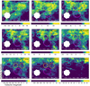 |
Fig. 1 CGPS H I emission distribution in velocity range from −46.0 to −67.4 km s−1. Each panel is an average of three consecutive velocity channel maps, with the central Local Standard of Rest (LSR) velocity indicated in its top right corner. The colour bars show the brightness temperature in kelvin. The four H I shells are outlined in orange (1), magenta (2), yellow (3), and cyan (4). H II regions are marked with red circles (see Sect. 4). |
Parameters derived for H I shells.
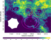 |
Fig. 2 Mean brightness temperature of CGPS H I emission averaged over velocity range from −56 to −59 km s−1. Colour ellipses mark the locations of the H I shells while the dashed line ellipses mark their outer boundaries. |
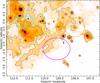 |
Fig. 3 IRIS 60 μm emission map in region under study. Contour levels are at 23 and 40 MJy/sr. Coloured ellipses mark the locations of the four H I shells. |
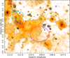 |
Fig. 4 Dust temperature map derived from emission distributions at 60 and 100 μm. The cyan (+) and blue (x) symbols mark the position of the H II regions from the WISE and Sharpless catalogues, respectively. These represent a subsample of the catalogued H II regions, whose selection criteria are described in Sect. 4. Contours are at 25 and 27 K. Coloured ellipses mark the locations of the four H I shells. |
HII regions from WISE and Sharpless catalogues.
5 Study of the H II regions
OB-type stars, particularly those earlier than B2, are the primary sources responsible for the ionisation of H II regions (see Table 2). In this section, we provide an overview of our approach to identifying such stars and analysing their association with the expanding shells. The methodological details are presented in the following subsections.
We begin by searching the literature for confirmed OB-type stars with known spectral classifications within the H II regions listed in Table 2. This enables us to select a representative sample of massive stars from which we derive characteristic standard parameters of colour excess and distance. We obtain these parameters using individual distances from Bailer-Jones et al. (2021) in combination with spectroscopic and photometric methods. Subsequently, based on this sample and the spatial distribution of the H II regions listed in Table 2, we define 13 areas (see Table 3) where we carry out photometric and astrometric analyses to identify additional massive star candidates. The position and size of these 13 areas are defined using all H II regions in Table 2. In one specific area, we use a smaller radius than the one listed in the Sharpless catalogue, as the original size extends beyond the area relevant to our stellar search.
5.1 Spectroscopic data and analysis
To find stars with confirmed spectral types (ST), we use the SIMBAD database, GOSSS, and the Galactic Wolf–Rayet Catalogue. While these spectral classifications come from multiple catalogues, their consistency and applicability are sufficient for our analysis. From these catalogues and databases, we collect a total of 27 OB-type stars with luminosity class (LC) V, of which 22 have Gaia DR3 counterparts. Of these 22 OB-type stars, 10 are confirmed massive stars.
Figure 5 shows the distribution of the 22 stars with confirmed spectral types and Gaia DR3 counterparts, where Gaia Gmag is on the x-axis and the distance from Bailer-Jones et al. (2021) is on the y-axis, including their associated uncertainties. The blue and pink dots represent spectral types earlier and later than B2, respectively. The figure shows that all ten confirmed massive stars lie between 2.2 and 3.2 kpc, as indicated by the dashed lines. Figure 6 shows a WISE colour image where coloured ellipses and circles represent the position and size of the H I shells, white circles indicate the H II regions, and red circles represent the 13 areas mentioned above. In this figure, the population of stars earlier than B2 appears clustered within the H II regions. Therefore, massive stars in the direction of the detected H I shells lie within that distance range. By contrast, stars later than B2 are more widely dispersed in both distance and position on the sky, showing typical characteristics of foreground field stars.
We use the entire sample of OB-type stars located between 2.2 and 3.2 kpc, which includes ten massive stars and three that are later than B 2. In an initial inspection, we detect that sources Gaia DR3 2014957793521124224 and 2013435042937606656 exhibit abnormal reddening and a high distance error, respectively; thus, they are not considered for estimations. The remaining 11 OB-type stars lie in four of the 13 areas (see Table 4). With this final sample, we conduct spectroscopic and photometric calculations to determine standard parameters of colour excess. The calculations are performed using absolute magnitudes and intrinsic colour calibration values obtained from the Gaia survey2 for main sequence (MS) spectral type (ST) classifications, and we apply linear interpolation for spectral types that are not listed in this survey. We combine these values with the Gaia photometric system GBP − GRP to compute the colour excesses and transform them to the standard E(B–V) using the relative absorption quantities given by Cardelli et al. (1989). For all calculations, we apply a normal value for the total-to-selective extinction ratio RV = 3.1. The spectral information for the sample of OB-type stars, along with the calculated results, is listed in Table 4, along with the distances given by Bailer-Jones et al. (2021).
For each of the four areas containing confirmed OB-type stars, we first perform the analysis using these confirmed massive sources to anchor the parameters. We compute the weighted average distance and its weighted standard deviation (![Mathematical equation: $\[\overline{Gaia_{dc}}\]$](/articles/aa/full_html/2026/03/aa54309-25/aa54309-25-eq6.png) ), as well as the average colour excess (
), as well as the average colour excess (![Mathematical equation: $\[\overline{E_{(B-V)}} c\]$](/articles/aa/full_html/2026/03/aa54309-25/aa54309-25-eq7.png) ). Based on these calculations – and taking into account high differential reddening and/or possible evolutionary effects – we set the highest and lowest values of E(B − V) as boundaries, denoted as E(B–V)M and E(B–V)m, respectively. Within these adopted boundaries, we then conduct the analysis of all 13 areas to search for additional massive star candidates, as described in Sect. 5.2.
). Based on these calculations – and taking into account high differential reddening and/or possible evolutionary effects – we set the highest and lowest values of E(B − V) as boundaries, denoted as E(B–V)M and E(B–V)m, respectively. Within these adopted boundaries, we then conduct the analysis of all 13 areas to search for additional massive star candidates, as described in Sect. 5.2.
Central coordinates and diameters of analysed areas.
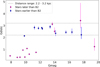 |
Fig. 5 Gaia Gmag versus distance (from Bailer-Jones et al. 2021) for stars located within H II regions listed in Table 2. Blue dots correspond to spectral types earlier than B2, and pink dots to spectral types later than B2. Vertical lines show the distance uncertainties. Dashed lines mark the adopted distance limits of 2.2 and 3.2 kpc. |
5.2 Massive star candidates
We next focus on identifying additional massive star candidates not previously catalogued in the literature. We perform this search in the 13 areas listed in Table 3 and also shown in Figure 6. As was previously explained, these areas are defined considering all catalogued H II regions listed in Table 2 and the distribution of confirmed massive stars.
We select additional massive star candidates using a criterion based on the photometric information provided by Gaia DR3, which we cross-correlate with 2MASS IR data and combine with the individual distances given by Bailer-Jones et al. (2021) from Gaia EDR3. The main-sequence reference values for the IR are given by Koornneef (1983) and Sung et al. (2013). The method is the same as that applied in previous works (Molina-Lera et al. 2016; Molina Lera et al. 2018; Molina Lera et al. 2019) and the description of the criterion is detailed in Suad et al. (2022). In summary, we use the photometric information to build two-colour diagrams (TCDs) in the IR (J − H) vs. (H − K) and colour-magnitude diagrams (CMDs) in the IR J vs. (J − H) and optical G vs. (GBP − GRP). In the optical CMD G vs. (GBP − GRP), we delimit a region by placing the MS reference curve at two different positions to select sources within an enclosed area. The positions of these curves are set using the previously mentioned standard parameters for distance and colour excess: 2.2 and 3.2 kpc (i.e. V° − Mv = 11.7–12.5), combined with E(B–V)M and E(B–V)m, respectively. These parameters, computed in the four areas with confirmed spectral types, are applied to all 13 areas to search for additional massive star candidates. For each selected massive star candidate, we calculate two representative values of the absolute magnitude in the Gaia G band (![Mathematical equation: $\[M_{G}^{B}\]$](/articles/aa/full_html/2026/03/aa54309-25/aa54309-25-eq8.png) and
and ![Mathematical equation: $\[M_{G}^{b}\]$](/articles/aa/full_html/2026/03/aa54309-25/aa54309-25-eq9.png) ). We derive these magnitudes by combining the upper and lower distance limits for each source, as given by Bailer-Jones et al. (2021), with E(B–V)M and E(B–V)m. The
). We derive these magnitudes by combining the upper and lower distance limits for each source, as given by Bailer-Jones et al. (2021), with E(B–V)M and E(B–V)m. The ![Mathematical equation: $\[M_{G}^{B}\]$](/articles/aa/full_html/2026/03/aa54309-25/aa54309-25-eq10.png) and
and ![Mathematical equation: $\[M_{G}^{b}\]$](/articles/aa/full_html/2026/03/aa54309-25/aa54309-25-eq11.png) values are then compared to those corresponding to known spectral types with LC V to establish their spectral classification. Finally, we select the sources whose
values are then compared to those corresponding to known spectral types with LC V to establish their spectral classification. Finally, we select the sources whose ![Mathematical equation: $\[M_{G}^{B}\]$](/articles/aa/full_html/2026/03/aa54309-25/aa54309-25-eq12.png) or
or ![Mathematical equation: $\[M_{G}^{b}\]$](/articles/aa/full_html/2026/03/aa54309-25/aa54309-25-eq13.png) correspond to absolute magnitudes of stars earlier than B2. Additionally, we examine the distribution of these sources in the IR TCD and CMD. Although these IR diagrams cannot definitively establish their nature, they serve as an effective diagnostic tool to exclude objects located outside the loci expected for early-type stars. No such cases have been found; consequently, the diagrams provide further support for the robustness of our selection.
correspond to absolute magnitudes of stars earlier than B2. Additionally, we examine the distribution of these sources in the IR TCD and CMD. Although these IR diagrams cannot definitively establish their nature, they serve as an effective diagnostic tool to exclude objects located outside the loci expected for early-type stars. No such cases have been found; consequently, the diagrams provide further support for the robustness of our selection.
The photometric diagrams are shown in Fig. A.1 in Appendix A. With coloured circles, we indicate sources situated within 2.2 and 3.2 kpc. Main-sequence calibration curves are represented by blue lines. The thinner blue lines in the optical CMD on both sides of the MS define the aforementioned area. Massive star candidates are depicted as blue circles, while small yellow circles represent potential low-mass stars. Sources that we discard are indicated with green circles, and grey dots represent sources at distances lower than 2.2 kpc or greater than 3.2 kpc. The figure also shows that all selected massive star candidates are distributed as expected in the photometric diagrams. Their parameters are shown in Table A.1 in Appendix A, along with the calculated absolute magnitudes and their previous spectral classifications (when available). Furthermore, our spectral type classification is consistent with those reported in the literature, reinforcing the validity of the criterion. Table 5 lists the parameters of the 11 areas, where each distance (Dist) represents the weighted average computed using the individual distances provided by Bailer-Jones et al. (2021). The table also includes the number of massive star candidates (n), the colour excesses (E(B–V)) and their adopted ranges (E(B–V)m, E(B–V)M), and the designation associated with each area shown in Fig. 6. We identify a total of 106 massive star candidates, including confirmed massive stars, in 11 of the 13 areas, located at a distance of 2.7 ± 0.5 kpc.
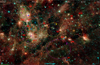 |
Fig. 6 Aladin WISE colour image. The coloured ellipses and circles indicate the position and size of the H I shells, as depicted in Fig. 1. The white circles show the H II regions, while the red ones show the 13 areas selected to search for massive star candidates. The blue and pink dots from Figure 6 are stars with confirmed spectral types, earlier and later than B2, respectively. |
Main parameters of massive stars with confirmed spectral types.
Main parameters of the 11 areas with associated massive star candidates.
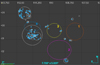 |
Fig. 7 Map showing spatial distribution of analysed structures. The coloured ellipses and circles indicate the position and size of the H I shells, as depicted in Fig. 1. The white circles show the H II regions, while the blue dots indicate the massive star candidates. |
6 Discussion
In the previous sections, we analysed four H I shells and 28 H II regions (grouped into 13 areas) projected along their borders, and identified several massive star candidates likely associated with most of them. Figure 7 shows the spatial correspondence between the massive star candidates and the H II regions listed in Table 2. Most H II regions host identified massive star candidates, while three very compact regions – G108.273–01.066/Sh2–147 (A6), G111.802+00.526 (A12), and Sh2–144 (A13) – do not. In A6 and A12, the ionising stars may still be too deeply embedded to be detected; however, both exhibit radio recombination line (RRL) emission with velocities consistent with those of the corresponding H I shells. In contrast, Sh2–144 (A13) shows neither RRL emission nor massive star candidates, and thus its association with the shells cannot be confirmed. Taking this into account, we consider that 27 H II regions, together with the four H I shells, are located at a common distance of 2.7 ± 0.5 kpc, as derived from the spectrophotometric distances of the identified massive stars.
Expanding H I shells are among the main sources of largescale compression in the interstellar medium, as their expansion sweeps up mass into dense, cold shell walls. Instabilities can develop within these walls (McClure-Griffiths et al. 2003), leading to the formation of high-density condensations, some of which may give rise to new stars. Several observational studies have provided evidence that star formation can be triggered by the expansion of H I shells (e.g. Elmegreen 2002; Oey et al. 2005; Dawson et al. 2011a,b; Suad et al. 2012, 2016, 2022). Within the scope of this work, the H II regions under study are located along the rims of the H I shells with a few located at overlapping edges of two structures, where shell interactions may occur. This spatial alignment suggests a possible causal link, which we explore in the following analysis.
If the expansion of the H I shells is indeed the mechanism responsible for triggering the formation of the ionising stars associated with the H II regions, a difference in age between these structures would be expected. According to Table 1, the estimated ages of the H I shells were found to range from 2.5 to 4.9 Myr. These values were obtained under the assumption of constant expansion velocity and do not take into account possible deceleration effects or projection uncertainties. All confirmed massive stars associated with the H II regions are of LC V, with ST ranging from O3.5 to B2. Their MS lifetimes (~3–22 Myr; Schaller et al. 1992) therefore set upper limits to the ages of the ionising sources. Since these lifetimes provide only upper limits, they do not allow us to establish whether the H I shells are older than the H II regions. To better constrain their relative ages, we can estimate dynamical timescales for the WISE H II regions (Table 2) using tdyn–HII = R/vexp. For the H II regions, we adopt typical expansion velocities of vexp ≃ 5–10 km s−1, representative of compact and evolved regions in a variety of ambient conditions (e.g. Dyson & Williams 1997). Using the angular radii listed in Table 2 and assuming a distance of 2.7 kpc, the resulting physical radii (R) range from 0.5 to 13.8 pc, yielding tdyn–HII ~ 0.05–2.7 Myr. These values are smaller than, or at most comparable to, the dynamical ages derived for the H I shells (2.5–4.9 Myr; Table 1). Although this comparison does not provide conclusive evidence for a causal link, it is consistent with a scenario in which the expansion of the H I shells may have played a role in triggering massive-star formation along their rims.
Several H II regions are located at the overlapping edges of the H I shells, corresponding to potential zones of shell interaction. As seen in Figs. 1 and 7, the H II regions in areas A2 and A6 lie at the interface between GS 108–0.4–057 (Shell 1) and GS 109–02–056 (Shell 2), while those in area A8 are found where GS 110–0.3–054 (Shell 3) intersects GS 111+0.0–060 (Shell 4). These observations support the idea that the collision of expanding shells may have triggered the formation of stars in these regions.
7 Summary
In this work, we analysed four expanding H I shells and their possible connection with 28 H II regions projected along their borders. The H I shells share a common velocity range (−46 to −67 km s−1) and show evidence of partial overlap, suggesting interactions between them. The H II regions, distributed along the rims and intersections of the shells, exhibit RRL velocities consistent with those of the H I gas, indicating a likely physical association.
Because kinematic distances are unreliable in the Perseus arm, we performed a spectrophotometric analysis based on Gaia data to identify massive star candidates and determine a common distance. We found 106 massive or candidate OB stars in 25 of the 28 H II regions, yielding an average distance of 2.7 ± 0.5 kpc, which we adopt for the entire complex.
Comparison of the dynamical ages of the H I shells (2.5–4.9 Myr) and those of the associated H II regions (≤2.7 Myr) suggests that the formation of the ionised regions could have been influenced by the H I shell expansion, although a causal connection cannot be firmly established.
These results suggest that the expansion and the interaction of the H I shells may both have played an important role in the recent star formation observed in this part of the Perseus arm.
Acknowledgements
We are particularly grateful to the anonymous referee for the thorough and constructive report, which greatly improved the clarity and quality of this work. LAS, SC, and SBC acknowledge support from CONICET grant PIP 11220220100211. JAML is co-funded by the European Union (Project 101183150 – OCEANS). LAS, JAML, and SC are Carrera del Investigador Científico del CONICET (Argentina) members. SBC is a doctoral fellow of CONICET, Argentina. The research presented in this paper has used data from the Canadian Galactic Plane Survey, a Canadian project with international partners, supported by the Natural Sciences and Engineering Research Council. This work makes use of data products from the Infrared Processing and Analysis Center/California Institute of Technology, funded by the National Aeronautics and Space Administration and the National Science Foundation. Data from the ESA mission Gaia, processed by the Gaia DPAC. Funding for the DPAC has been provided by national institutions, in particular the institutions participating in the Gaia Multilateral Agreement.
References
- Anderson, L. D., Zavagno, A., Deharveng, L., et al. 2012, A&A, 542, A10 [NASA ADS] [CrossRef] [EDP Sciences] [Google Scholar]
- Anderson, L. D., Bania, T. M., Balser, D. S., et al. 2014, ApJS, 212, 1 [Google Scholar]
- Bailer-Jones, C. A. L., Rybizki, J., Fouesneau, M., Demleitner, M., & Andrae, R. 2021, AJ, 161, 147 [Google Scholar]
- Cardelli, J. A., Clayton, G. C., & Mathis, J. S. 1989, ApJ, 345, 245 [Google Scholar]
- Chernin, A. D., Efremov, Y. N., & Voinovich, P. A. 1995, MNRAS, 275, 313 [NASA ADS] [CrossRef] [Google Scholar]
- Dawson, J. R. 2013, PASA, 30, e025 [NASA ADS] [CrossRef] [Google Scholar]
- Dawson, J. R., McClure-Griffiths, N. M., Dickey, J. M., & Fukui, Y. 2011a, ApJ, 741, 85 [Google Scholar]
- Dawson, J. R., McClure-Griffiths, N. M., Kawamura, A., et al. 2011b, ApJ, 728, 127 [NASA ADS] [CrossRef] [Google Scholar]
- Dawson, J. R., McClure-Griffiths, N. M., Wong, T., et al. 2013, ApJ, 763, 56 [NASA ADS] [CrossRef] [Google Scholar]
- Dawson, J. R., Ntormousi, E., Fukui, Y., Hayakawa, T., & Fierlinger, K. 2015, ApJ, 799, 64 [NASA ADS] [CrossRef] [Google Scholar]
- Dyson, J. E., & Williams, D. A. 1997, The physics of the Interstellar Medium (The Physics of the Interstellar Medium), 2nd edn. (Bristol: Institute of Physics Publishing), eds. J. E. Dyson & D. A. Williams, The Graduate Series in Astronomy [Google Scholar]
- Egorov, O. V., Lozinskaya, T. A., Moiseev, A. V., & Smirnov-Pinchukov, G. V. 2018, MNRAS, 478, 3386 [NASA ADS] [CrossRef] [Google Scholar]
- Ehlerová, S., & Palouš, J. 2005, A&A, 437, 101 [NASA ADS] [CrossRef] [EDP Sciences] [Google Scholar]
- Ehlerová, S., & Palouš, J. 2013, A&A, 550, A23 [NASA ADS] [CrossRef] [EDP Sciences] [Google Scholar]
- Elmegreen, B. G. 2002, in Extragalactic Star Clusters, 207, eds. D. P. Geisler, E. K. Grebel, & D. Minniti, 390 [Google Scholar]
- Foster, T., & MacWilliams, J. 2006, ApJ, 644, 214 [NASA ADS] [CrossRef] [Google Scholar]
- Fujii, K., Mizuno, N., Dawson, J. R., et al. 2021, MNRAS, 505, 459 [NASA ADS] [CrossRef] [Google Scholar]
- Gaczkowski, B., Roccatagliata, V., Flaischlen, S., et al. 2017, A&A, 608, A102 [NASA ADS] [CrossRef] [EDP Sciences] [Google Scholar]
- Heiles, C. 1979, ApJ, 229, 533 [NASA ADS] [CrossRef] [Google Scholar]
- Inoue, T., & Inutsuka, S.-i. 2008, ApJ, 687, 303 [NASA ADS] [CrossRef] [Google Scholar]
- Inoue, T., & Inutsuka, S.-i. 2009, ApJ, 704, 161 [NASA ADS] [CrossRef] [Google Scholar]
- Inutsuka, S.-i., Inoue, T., Iwasaki, K., & Hosokawa, T. 2015, A&A, 580, A49 [NASA ADS] [CrossRef] [EDP Sciences] [Google Scholar]
- Kim, C.-G., & Ostriker, E. C. 2015, ApJ, 802, 99 [NASA ADS] [CrossRef] [Google Scholar]
- Koornneef, J. 1983, A&AS, 51, 489 [Google Scholar]
- Krause, M. G. H., Burkert, A., Diehl, R., et al. 2018, A&A, 619, A120 [NASA ADS] [CrossRef] [EDP Sciences] [Google Scholar]
- McClure-Griffiths, N. M., Dickey, J. M., Gaensler, B. M., & Green, A. J. 2002, ApJ, 578, 176 [NASA ADS] [CrossRef] [Google Scholar]
- McClure-Griffiths, N. M., Dickey, J. M., Gaensler, B. M., & Green, A. J. 2003, ApJ, 594, 833 [Google Scholar]
- McCray, R., & Kafatos, M. 1987, ApJ, 317, 190 [NASA ADS] [CrossRef] [Google Scholar]
- Miville-Deschênes, M.-A., & Lagache, G. 2005, ApJS, 157, 302 [Google Scholar]
- Molina-Lera, J. A., Baume, G., Gamen, R., Costa, E., & Carraro, G. 2016, A&A, 592, A149 [NASA ADS] [CrossRef] [EDP Sciences] [Google Scholar]
- Molina Lera, J. A., Baume, G., & Gamen, R. 2018, MNRAS, 480, 2386 [NASA ADS] [CrossRef] [Google Scholar]
- Molina Lera, J. A., Baume, G., & Gamen, R. 2019, MNRAS, 488, 2158 [NASA ADS] [CrossRef] [Google Scholar]
- Ntormousi, E., Burkert, A., Fierlinger, K., & Heitsch, F. 2011, ApJ, 731, 13 [NASA ADS] [CrossRef] [Google Scholar]
- Ntormousi, E., Dawson, J. R., Hennebelle, P., & Fierlinger, K. 2017, A&A, 599, A94 [NASA ADS] [CrossRef] [EDP Sciences] [Google Scholar]
- Oey, M. S., Watson, A. M., Kern, K., & Walth, G. L. 2005, AJ, 129, 393 [NASA ADS] [CrossRef] [Google Scholar]
- O’Neill, T. J., Zucker, C., Goodman, A. A., & Edenhofer, G. 2024, ApJ, 973, 136 [NASA ADS] [CrossRef] [Google Scholar]
- Reid, M. J., Menten, K. M., Brunthaler, A., et al. 2014, ApJ, 783, 130 [Google Scholar]
- Rosslowe, C. K., & Crowther, P. A. 2015, MNRAS, 447, 2322 [NASA ADS] [CrossRef] [Google Scholar]
- Schaller, G., Schaerer, D., Meynet, G., & Maeder, A. 1992, A&AS, 96, 269 [Google Scholar]
- Schnee, S. L., Ridge, N. A., Goodman, A. A., & Li, J. G. 2005, ApJ, 634, 442 [NASA ADS] [CrossRef] [Google Scholar]
- Sharpless, S. 1959, ApJS, 4, 257 [Google Scholar]
- Skrutskie, M. F., Cutri, R. M., Stiening, R., et al. 2006, AJ, 131, 1163 [NASA ADS] [CrossRef] [Google Scholar]
- Sota, A., Maíz Apellániz, J., Morrell, N., et al. 2014, ApJS, 211, 10 [NASA ADS] [CrossRef] [Google Scholar]
- Suad, L. A., Cichowolski, S., Arnal, E. M., & Testori, J. C. 2012, A&A, 538, A60 [NASA ADS] [CrossRef] [EDP Sciences] [Google Scholar]
- Suad, L. A., Caiafa, C. F., Arnal, E. M., & Cichowolski, S. 2014, A&A, 564, A116 [NASA ADS] [CrossRef] [EDP Sciences] [Google Scholar]
- Suad, L. A., Cichowolski, S., Noriega-Crespo, A., et al. 2016, A&A, 585, A154 [NASA ADS] [CrossRef] [EDP Sciences] [Google Scholar]
- Suad, L. A., Caiafa, C. F., Cichowolski, S., & Arnal, E. M. 2019, A&A, 624, A43 [NASA ADS] [CrossRef] [EDP Sciences] [Google Scholar]
- Suad, L. A., Molina Lera, J. A., & Cichowolski, S. 2022, A&A, 668, A44 [NASA ADS] [CrossRef] [EDP Sciences] [Google Scholar]
- Sung, H., Lim, B., Bessell, M. S., et al. 2013, J. Korean Astron. Soc., 46, 103 [NASA ADS] [CrossRef] [Google Scholar]
- Taylor, A. R., et al. 2003, AJ, 125, 3145 [NASA ADS] [CrossRef] [Google Scholar]
- Tenorio-Tagle, G. 1981, A&A, 94, 338 [NASA ADS] [Google Scholar]
- Tenorio-Tagle, G., & Bodenheimer, P. 1988, ARA&A, 26, 145 [Google Scholar]
- van Leeuwen, F., de Bruijne, J., Babusiaux, C., et al. 2022, Gaia DR3 documentation, European Space Agency; Gaia Data Processing and Analysis Consortium [Google Scholar]
- Weaver, R., McCray, R., Castor, J., Shapiro, P., & Moore, R. 1977, ApJ, 218, 377 [Google Scholar]
- Wenger, M., Ochsenbein, F., Egret, D., et al. 2000, A&AS, 143, 9 [NASA ADS] [Google Scholar]
- Xu, Y., Reid, M. J., Zheng, X. W., & Menten, K. M. 2006, Science, 311, 54 [NASA ADS] [CrossRef] [Google Scholar]
- Yamada, R. I., Sano, H., Tachihara, K., et al. 2024, PASJ, 76, 895 [Google Scholar]
- Zucker, C., Speagle, J. S., Schlafly, E. F., et al. 2019, ApJ, 879, 125 [NASA ADS] [CrossRef] [Google Scholar]
- Zucker, C., Goodman, A. A., Alves, J., et al. 2022, Nature, 601, 334 [NASA ADS] [CrossRef] [Google Scholar]
Appendix A Additional figures and table
This appendix presents Figure A.1 and Table A.1 referred to in Sect. 5.2.
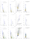 |
Fig. A.1 Photometric diagrams for 11 areas containing massive-star candidates (area label at top of each panel). The MS locus is the thick blue line; thin blue lines enclose the selected region (Sect. 5). Coloured circles mark sources at 2.2–3.2 kpc; grey dots are outside this range. Massive-star candidates are shown as blue circles (labels give ST). Potential low-mass stars are yellow; discarded sources are green. |
Massive star candidates in each of 11 areas.
All Tables
All Figures
|
Fig. 1 CGPS H I emission distribution in velocity range from −46.0 to −67.4 km s−1. Each panel is an average of three consecutive velocity channel maps, with the central Local Standard of Rest (LSR) velocity indicated in its top right corner. The colour bars show the brightness temperature in kelvin. The four H I shells are outlined in orange (1), magenta (2), yellow (3), and cyan (4). H II regions are marked with red circles (see Sect. 4). |
| In the text | |
|
Fig. 2 Mean brightness temperature of CGPS H I emission averaged over velocity range from −56 to −59 km s−1. Colour ellipses mark the locations of the H I shells while the dashed line ellipses mark their outer boundaries. |
| In the text | |
|
Fig. 3 IRIS 60 μm emission map in region under study. Contour levels are at 23 and 40 MJy/sr. Coloured ellipses mark the locations of the four H I shells. |
| In the text | |
|
Fig. 4 Dust temperature map derived from emission distributions at 60 and 100 μm. The cyan (+) and blue (x) symbols mark the position of the H II regions from the WISE and Sharpless catalogues, respectively. These represent a subsample of the catalogued H II regions, whose selection criteria are described in Sect. 4. Contours are at 25 and 27 K. Coloured ellipses mark the locations of the four H I shells. |
| In the text | |
|
Fig. 5 Gaia Gmag versus distance (from Bailer-Jones et al. 2021) for stars located within H II regions listed in Table 2. Blue dots correspond to spectral types earlier than B2, and pink dots to spectral types later than B2. Vertical lines show the distance uncertainties. Dashed lines mark the adopted distance limits of 2.2 and 3.2 kpc. |
| In the text | |
|
Fig. 6 Aladin WISE colour image. The coloured ellipses and circles indicate the position and size of the H I shells, as depicted in Fig. 1. The white circles show the H II regions, while the red ones show the 13 areas selected to search for massive star candidates. The blue and pink dots from Figure 6 are stars with confirmed spectral types, earlier and later than B2, respectively. |
| In the text | |
|
Fig. 7 Map showing spatial distribution of analysed structures. The coloured ellipses and circles indicate the position and size of the H I shells, as depicted in Fig. 1. The white circles show the H II regions, while the blue dots indicate the massive star candidates. |
| In the text | |
|
Fig. A.1 Photometric diagrams for 11 areas containing massive-star candidates (area label at top of each panel). The MS locus is the thick blue line; thin blue lines enclose the selected region (Sect. 5). Coloured circles mark sources at 2.2–3.2 kpc; grey dots are outside this range. Massive-star candidates are shown as blue circles (labels give ST). Potential low-mass stars are yellow; discarded sources are green. |
| In the text | |
Current usage metrics show cumulative count of Article Views (full-text article views including HTML views, PDF and ePub downloads, according to the available data) and Abstracts Views on Vision4Press platform.
Data correspond to usage on the plateform after 2015. The current usage metrics is available 48-96 hours after online publication and is updated daily on week days.
Initial download of the metrics may take a while.