| Issue |
A&A
Volume 707, March 2026
|
|
|---|---|---|
| Article Number | A33 | |
| Number of page(s) | 14 | |
| Section | Stellar structure and evolution | |
| DOI | https://doi.org/10.1051/0004-6361/202555276 | |
| Published online | 25 February 2026 | |
Characteristics of the high-frequency humps in the black hole X-ray binary Swift J1727.8–1613
1
Key Laboratory for Particle Astrophysics, Institute of High Energy Physics, Chinese Academy of Sciences 19B Yuquan Road Beijing 100049, China
2
University of Chinese Academy of Sciences, Chinese Academy of Sciences Beijing 100049, China
3
Department of Physics and Astronomy, University of Southampton Highfield Southampton SO17 1BJ, UK
4
School of Physics and Optoelectronic Engineering, Shandong University of Technology Zibo 255000, China
5
Key Laboratory of Space Astronomy and Technology, National Astronomical Observatories, Chinese Academy of Sciences Beijing 100101, China
★ Corresponding authors: This email address is being protected from spambots. You need JavaScript enabled to view it.
; This email address is being protected from spambots. You need JavaScript enabled to view it.
Received:
23
April
2025
Accepted:
6
January
2026
Abstract
We present a detailed timing analysis of the two high-frequency humps observed in the power density spectrum of Swift J1727.8–1613 up to 100 keV, using data from the Hard X-ray Modulation Telescope (Insight-HXMT). Our analysis reveals that the characteristic frequencies of the humps increase with energy up to ∼30 keV, followed by a plateau at higher energies. The fractional rms amplitudes of the humps increase with energy, reaching approximately 15% in the 50–100 keV band. The lag spectrum of the hump is characterized primarily by a soft lag that varies with energy. Our results suggest that the high-frequency humps originate from a corona close to the black hole. Additionally, by applying the relativistic precession model, we constrain the mass of Swift J1727.8–1613 to 2.84 < M/M⊙ < 120.01 and the spin to 0.14 < a < 0.43 from the full-energy-band dataset, using triplets composed of a type-C quasiperiodic oscillation and two high-frequency humps. When considering only the high-energy bands with stable characteristic frequencies, we derive additional constraints of 2.84 < M/M⊙ < 13.98 and 0.14 < a < 0.40.
Key words: stars: black holes / X-rays: binaries / X-rays: individuals: Swift J1727.8–1613
© The Authors 2026
 Open Access article, published by EDP Sciences, under the terms of the Creative Commons Attribution License (https://creativecommons.org/licenses/by/4.0), which permits unrestricted use, distribution, and reproduction in any medium, provided the original work is properly cited.
This article is published in open access under the Subscribe to Open model. This email address is being protected from spambots. You need JavaScript enabled to view it. to support open access publication.
1. Introduction
Black hole low-mass X-ray binaries (BH-LMXBs) in outbursts usually exhibit fast X-ray aperiodic variability on a wide range of timescales (see reviews by Remillard & McClintock 2006; Done et al. 2007). Fourier analysis serves as an effective and intuitive approach for examining these complex timing variations. In a typical power density spectrum (PDS) of BH-LMXBs, several narrow peaks, known as quasiperiodic oscillations (QPOs), are commonly observed alongside a broadband noise (BBN) continuum (see reviews by Belloni & Motta 2016; Ingram & Motta 2019). Based on their frequencies, QPOs can be categorized into two main groups: low-frequency QPOs (LFQPOs, e.g., Samimi et al. 1979; van der Klis et al. 1985; Vikhlinin et al. 1995; Wijnands et al. 1999; Homan et al. 2001; Remillard et al. 2002b; Casella et al. 2005; Motta et al. 2011), which have frequencies ranging from 0.1 to 30 Hz, and high-frequency QPOs (HFQPOs, e.g., Morgan et al. 1997; Remillard et al. 1999; Psaltis et al. 1999; Strohmayer 2001; Belloni et al. 2012; Méndez et al. 2013), typically ranging from 40 to 450 Hz.
Low-frequency QPOs have been observed in almost all BH-LMXBs. Based on the shape of the PDS and the spectral state during which the QPOs are detected, LFQPOs can be further categorized into types A, B, and C (Remillard et al. 2002b; Casella et al. 2005). The origins of LFQPOs are primarily attributed to two classes of models: accretion disk instability models (Kato 1990; Molteni et al. 1996; Tagger & Pellat 1999) and geometrical effect models. The latter includes, for example, Lense-Thirring precession of the hot inner flow (Ingram et al. 2009) or the precession of the jet base (Stevens & Uttley 2016; Ma et al. 2021). Evidence suggests that type-C QPOs have a geometric origin, as indicated by the inclination-dependent fractional rms of the QPOs and the modulation of the iron line with QPO phase (Motta et al. 2015; Ingram et al. 2016). However, models related to geometrical effects still encounter considerable challenges, both theoretically and observationally (Marcel & Neilsen 2021; Zhao et al. 2024).
High-frequency QPOs have been observed in only a limited number of BH-LMXBs (e.g., Strohmayer 2001; Belloni et al. 2012; Méndez et al. 2013). The frequency of the HFQPOs usually occurs at specific values and does not change significantly with luminosity (Remillard et al. 2002a, 2006). In some sources, double peaks have been observed, with the frequency ratio consistently approximating 3:2 (Strohmayer 2001; Remillard et al. 2002a; Homan et al. 2005). Furthermore, HFQPOs are generally very weak, with fractional rms amplitudes typically below 5% (Belloni et al. 2012). Numerous theoretical models have been proposed to explain the underlying mechanisms of HFQPOs, although their physical origin remains highly debated. Abramowicz & Kluźniak (2001) proposed a resonant mechanism, specifically accounting for the observed 3:2 frequency ratio. However, the robustness of this frequency ratio remains uncertain due to the limited number of detections. Another widely used model to explain HFQPOs is the relativistic precession model (RPM; Stella & Vietri 1998, 1999; Stella et al. 1999). The RPM associates the nodal precession frequency (νnod), the periastron precession frequency (νper), and the orbital frequency (νϕ) at the same radius with the type-C QPO, the lower HFQPO, and the upper HFQPO frequency, respectively. When HFQPO pairs and a type-C QPO are observed simultaneously, the mass and spin of the black hole can be determined analytically using the RPM. This approach has been successfully applied to estimate the mass and spin parameters of several BH-LMXBs (Motta et al. 2014a,b; du Buisson et al. 2019; Motta et al. 2022).
Among the components of BBN, the high-frequency humps, characterized by frequencies exceeding approximately 30 Hz, are generally the highest frequency features detected in the PDS of BH-LMXBs. These humps play a critical role in investigating the short-timescale dynamics of matter in the innermost regions around black holes. Such humps have been observed in numerous sources (Nowak 2000; Trudolyubov 2001; Belloni et al. 2002; Kalemci et al. 2003; Motta et al. 2014a,b; Bhargava et al. 2021; Alabarta et al. 2022; Motta et al. 2022). The characteristic frequencies of the humps exhibit a strong correlation with the frequency of the LFQPO (Psaltis et al. 1999; Fogantini et al. 2025). The fractional rms amplitudes of the humps typically increase with photon energy (Zhang et al. 2022, 2024). In the case of GRS 1915+105, the rms amplitudes of the humps show a positive correlation with the corona temperature and an anticorrelation with the radio flux (Méndez et al. 2022; Zhang et al. 2022). This suggests that the humps serve as an indicator of accretion energy distribution. When the humps are strong, the majority of the accretion energy is channeled into the corona rather than being transferred to the jet. Zhang et al. (2022) further proposed that the humps and the HFQPO in GRS 1915+105 originate from the same variability component, with the coherence of this component being determined by the properties of the corona.
The bright new X-ray transient Swift J1727.8–1613 was discovered by Swift/BAT on August 24, 2023 (Negoro et al. 2023; Kennea & Swift Team 2023). Dynamical measurements have confirmed the compact object to be a black hole with a mass of M > 3.12 ± 0.10 M⊙ (Mata Sánchez et al. 2025). An extremely high spin value of 0.98 was obtained from reflection modeling (Liu et al. 2024). The distance to Swift J1727.8–1613 was initially estimated to be d = 2.7 ± 0.3 kpc using several empirical methods (Mata Sánchez et al. 2024). However, Burridge et al. 2025 suggested an increased distance of  kpc. Additionally, Wood et al. (2024) identified a bright core and a large, two-sided, asymmetrical, resolved jet using the VLBA and LBA observations. They constrained the jet speed to β ≥ 0.27 and the jet inclination to i ≤ 74°.
Yu et al. (2024) conducted a comprehensive analysis of the evolution of the X-ray variability in Swift J1727.8–1613 using Insight-HXMT observations. They detected prominent type-C QPO with frequencies ranging from 0.1 Hz to 8 Hz. Additionally, significant high-frequency humps were observed in the PDS, whose frequencies highly correlate with QPO frequencies. In this study, we present a detailed investigation of the evolution of the high-frequency humps and their energy-dependent properties up to 100 keV using Insight-HXMT observations. Furthermore, we determine the black hole mass and spin in Swift J1727.8–1613 by applying the RPM. In Section 2, we introduce our data selection and reduction methodology. We present our data analysis and results in Section 3. In Section 4, we discuss our main findings.
2. Observation and data reduction
Insight-HXMT is renowned for its broad energy range, spanning from 1 keV to 250 keV, achieved through the utilization of three distinct telescopes: the High Energy X-ray telescope (HE, 20–250 keV, Liu et al. 2020), the Medium Energy X-ray telescope (ME, 5–30 keV, Cao et al. 2020), and the Low Energy X-ray telescope (LE, 1–15 keV, Chen et al. 2020). Insight-HXMT observed the outburst of Swift J1727.8–1613 from August 25 to October 4, 2023, with a high cadence over a total duration exceeding one month. We processed all the data using the Insight-HXMT Data Analysis Software v2.06. The good time interval (GTI) filtering criteria were based on the default standards recommended by the Insight-HXMT team: (1) an Earth elevation angle larger than 10°; (2) a pointing offset angle less than 0.04°; (3) a geomagnetic cutoff rigidity value higher than 8 GV; and (4) at least 300 s before and after the South Atlantic Anomaly passage.
In Fig. 1, we show the LE 2–10 keV, ME 10–23 keV, and HE 23–100 keV light curves for the outburst of Swift J1727.8–1613. The LE light curve exhibits a rapid rise followed by an exponential decay, alongside several flares occurring between MJD 60197 and MJD 60220. Notably, these flares are not observed in the ME and HE light curves. In Fig. 2, we plot the hardness-intensity diagram (HID). The hardness is defined as the ratio of the count rate between the 2–3 keV and 3–7 keV energy bands, while the intensity corresponds to the count rate in the 2–7 keV band.
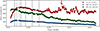 |
Fig. 1. Insight-HXMT LE 2–10 keV, ME 10–23 keV, and HE 23–100 keV light curves of Swift J1727.8–1613 during its 2023 outburst. Each data point corresponds to an exposure ID. The shaded regions mark the data groups selected for our timing analysis. |
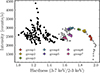 |
Fig. 2. Insight-HXMT HID of Swift J1727.8–1613 during its 2023 outburst. Each data point corresponds to an exposure ID. The different colored points represent the data groups selected for our timing analysis. |
In this study, we focus on the analysis of high-frequency humps, which were only detected in the PDS prior to the flaring state (see Yu et al. 2024). For our analysis, we selected seven data groups by merging several adjacent ExpIDs that exhibit consistent source flux, spectral hardness ratios, and PDS shapes to ensure robust statistical results. To achieve this, we applied the following criteria: (1) The variation in the count rate for each detector must remain within 0.05 times the average value1. (2) The variation in the hardness ratio must be less than 0.02. (3) The variation in the QPO frequency must remain within 0.1 Hz. The total effective exposure time for each group exceeds 6 ks. A detailed log of the observations analyzed in this study is listed in Table 1. The data groups are also marked in Figs. 1 and 2.
Log of the seven data groups selected for our timing analysis.
3. Data analysis and results
3.1. Power density spectrum and cross spectrum
For each group, we produced averaged PDS in different energy bands using a time interval of 128 s and a time resolution of 1 ms. The resulting PDS were normalized in units of (rms/mean)2 Hz−1 (Belloni & Hasinger 1990), and the Poisson noise level estimated from the power between 200 and 500 Hz was subtracted. To account for background, we applied a correction by multiplying the power by  , where N and S represent the count rates of the background and the source, respectively. We modeled the PDS using a combination of multiple Lorentzian functions.
In the upper-left panel of Fig. 3, we show a representative PDS of Group 3, calculated in the 4–10 keV band. The PDS can be well described by a model comprising seven Lorentzian functions. A sharp type-C QPO is prominently observed, accompanied by its second-harmonic peak. The low-frequency noise was fit using three Lorentzian functions. Additionally, two high-frequency humps are significantly detected; they are denoted as Ll and Lh. We note that the component Lh was not detected in the PDS analyzed by Yu et al. (2024), as their study was confined to a frequency range below 50 Hz.
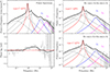 |
Fig. 3. Upper-left panel: PDS in the 4–10 keV energy band. Lower-left panel: Phase lag vs. Fourier frequency (phase-lag spectrum) together with the derived model obtained from the fits to the power and cross spectra. Upper-right and lower-right panels: Real and imaginary parts of the cross spectrum calculated for the 4–10 keV band with respect to the 2–4 keV band. For the fitting and the plot, we rotated the cross-vector by 45°. We modeled the PDS using seven Lorentzian functions. Additionally, we fit the real and imaginary parts of the cross spectrum by fixing the frequency and FWHM of each Lorentzian to the values derived from the best-fit model of the PDS. Type-C QPO corresponds to the Lorentzian function used to fit the type-C QPO, while Ll and Lh represent the Lorentzian functions fitting the two high-frequency humps. |
To determine the lags of the variability components identified in the PDS, we also computed averaged cross spectra2 between different energy bands using the same time interval and time resolution as for PDS. Traditionally, the lag of a BBN component or QPO is measured as the ratio of the average real and imaginary parts of the cross spectrum within the selected frequency range (typically  ; see, e.g., van der Klis et al. 1987). This method assumes that the component of interest dominates the power and cross spectra over the frequency range of interest. However, in cases where other components contribute significantly to the power and cross spectra in the selected frequency range, this method becomes ineffective. To measure the lags of weak variability components, Méndez et al. (2024) introduced a novel method based on simultaneously fitting the PDS and the real and imaginary parts of the cross spectrum, using a combination of Lorentzian functions. This method assumes that the power and cross spectra of the source consist of multiple components coherent across different energy bands but incoherent with each other. The constant phase-lag model proposed by Méndez et al. (2024) assumes that the phase lags of individual Lorentzian components are constant with Fourier frequency. This approach simplifies the computation of phase lags by modeling the real and imaginary components of the cross spectrum using multiple Lorentzian functions3. We refer readers to Méndez et al. (2024) for the details of the method.
In the upper-right and lower-right panels of Fig. 3, we show the real and imaginary parts of the cross spectrum for Group 3 in the 4–10 keV band, with the 2–4 keV band as reference. In the lower-left panel of Fig. 3, we show the phase lag versus Fourier frequency. Given that the power of the imaginary part of the cross spectrum is significantly smaller than that of the real part, we rotated the cross-vector by 45° to enhance the stability of the fitting process. We simultaneously fit the real and imaginary parts of the cross spectrum using the same number of Lorentzian components as those employed in the PDS fitting, fixing the frequency and full width at half-maximum (FWHM) of each Lorentzian to the values derived from the PDS fits, and assuming the constant phase-lag model as described in Méndez et al. (2024) and Jin et al. (2025). Using this method, we obtained the phase lags associated with each variability component.
3.2. Energy-dependent properties of the QPO and high-frequency humps
To examine the energy-dependent properties of the variability components, we generated the PDSs for such different energy bands as LE (2–4 keV, 4–10 keV), ME (10–14 keV, 14–23 keV), and HE (23–35 keV, 35–50 keV, 50–100 keV). Additionally, we computed the cross spectrum for each energy band, using the 2–4 keV band as reference. Following the previously described method, we obtained the characteristic frequency (νmax4), fractional rms amplitude, and phase lag of type-C QPO, Ll, and Lh in each energy band.
In Fig. 4, we show the characteristic frequency (νmax) and fractional rms amplitude of type-C QPO, Ll, and Lh as a function of photon energy. We observed that the characteristic frequency of the type-C QPO remains constant across different energy bands. In contrast, its fractional rms amplitude exhibits a rapid increase with energy below 25 keV, but remains more or less constant at higher energies. This is consistent with the findings reported in Yang et al. (2024) and Yu et al. (2024). The behaviors of the two high-frequency humps, Ll and Lh, exhibit notable similarities. Their characteristic frequencies increase with energy up to 25 keV, then stabilize. Additionally, their fractional rms amplitudes consistently increase with energy toward higher energy bands, although some scatter is observed for Lh in the low-energy bands.
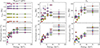 |
Fig. 4. Energy dependence of the characteristic frequency and fractional rms of the type-C QPO and the two high-frequency humps (Ll and Lh) for each data group. The color scheme for the seven data groups follows that highlighted in Fig. 2. |
In Fig. 5, we show the phase lags of the type-C QPO and Ll as a function of photon energy. The phase lag of the type-C QPO shows slight hard lags in most cases and remains consistent across energy bands without significant variation. However, the lag spectrum of Ll is characterized primarily by a soft lag that varies with energy. Owing to the limited signal-to-noise ratio, the phase lag associated with both Ll in the 50–100 keV range and Lh cannot be constrained well.
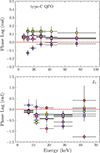 |
Fig. 5. Energy dependence of the phase lag of the type-C QPOs and Ll for each data group. The color scheme for the seven data groups follows that highlighted in Fig. 2. |
3.3. Measuring the mass and spin of the black hole with the relativistic precession model
The RPM links three types of QPOs observed in BH-LMXBs to a combination of the fundamental frequencies of particle motion. Type-C QPOs are associated with the nodal precession frequency (νnod). The lower and upper HFQPOs correspond to the periastron precession frequency (νper) and orbital frequency (νϕ), respectively (Stella & Vietri 1998, 1999; Stella et al. 1999; Motta et al. 2014a). Assuming that these frequencies originate from the same radius (r), the orbital frequency, the periastron precession frequency, and the nodal precession frequency can be expressed as
 (1)
(1)
 (2)
(2)
 (3)
(3)
where M is the black hole mass and a is the dimensionless spin parameter. If all three QPOs are detected simultaneously, we can determine the mass and spin of the black hole. Furthermore, Ingram & Motta (2014) found the analytical solution to the RPM system as follows:
 (4)
(4)
 (5)
(5)
where Γ and Δ are given by
 (6)
(6)
 (7)
(7)
From this, the spin and mass can be determined from equations (5) and (1).
Motta et al. (2014a) and Motta et al. (2014b) investigated the HFQPOs and high-frequency humps of GRO J1655–40 and XTE J1550–564. Their research findings indicate that the characteristic frequencies of the lower and upper high-frequency humps align with the periastron precession and orbital frequencies predicted by the RPM. Zhang et al. (2022) further proposed that the high-frequency humps and the HFQPOs may originate from the same variability component, with the coherence of this variability being influenced by the properties of the corona. Therefore, in principle, triplets consisting of two high-frequency humps and a type-C QPO can be used to constrain the mass and spin of the black hole. Bhargava et al. (2021) applied this method to the BH-LMXB MAXI J1820+070 and estimated its spin to be  .
.
In Swift J1727.8–1613, we detected two prominent high-frequency humps, Ll and Lh, in each analyzed data group, accompanied by a type-C QPO. Yu et al. (2024) found that the frequency of Ll exhibits a strong correlation with the frequency of the type-C QPO, consistent with the Psaltis-Belloni-van der Klis (PBK) relation (Psaltis et al. 1999). Meanwhile, we found that the characteristic frequencies of the two high-frequency humps, Ll and Lh, are also correlated, as shown in Fig. 6. Their relationship can be fit with an exponential function as νh = (0.71 ± 0.38)νl1.52 ± 0.18.
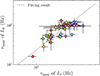 |
Fig. 6. Relationship between the characteristic frequencies of the high-frequency humps, Ll and Lh. The dashed line represents the best-fit using an exponential function. |
We then employed the RPM to estimate the mass and spin of the black hole in Swift J1727.8–1613 using triplets composed of two high-frequency humps and a type-C QPO observed in each data group and energy band. Following Motta et al. (2014a), we calculated the errors using a Monte Carlo method. We simulated 105 sets of three frequencies measured from the PDS of Swift J1727.8–1613. We then solved the RPM equations for each set of the three frequencies and obtained distributions of mass, spin, and radius. By fitting the distributions of these parameters, we derived measurements of the mass and spin. Fig. 7 shows the mass and spin predicted by each of the triplets used in our analysis. The parameter distributions are represented as histograms located at the top and right of the figure. Using the full-energy-band dataset, the mass and spin distributions are constrained within the ranges of 2.84 < M/M⊙ < 120.01 and 0.14 < a < 0.43, with median values of 10.30 M⊙ and 0.25, respectively. When considering only the high-energy bands (greater than 25 keV), where the characteristic frequencies of the two humps tend to stabilize, the mass and spin distributions are determined to be 2.84 < M/M⊙ < 13.98 and 0.14 < a < 0.40, with median values of 7.12 M⊙ and 0.20, respectively. Consequently, in Fig. 8, we identify the Type-C QPO and the two high-frequency humps (Ll and Lh) as the nodal precession frequency, periastron precession frequency, and orbital frequency, respectively. We also present mass and spin measurements of 7.12 M⊙ and 0.20 obtained via the RPM from the high-energy dataset and plot these values as a function of the nodal precession frequency. It is apparent that most of the characteristic frequencies match the frequencies predicted by the best-fitting RPM well.
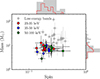 |
Fig. 7. Mass and spin estimates derived from the RPM using the triplets composed of a type-C QPO and two high-frequency humps. The gray points represent the spin and mass values obtained using the triples from the energy bands below 23 keV. The distributions of the spin and mass can be seen at the top and to the right of the figure. The gray areas correspond to the distribution of the full-energy bands, while the dashed red lines represent the distribution considering only the high-energy bands above 23 keV. |
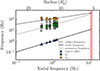 |
Fig. 8. Nodal precession frequency (solid line), periastron precession frequency (dotted line), and orbital frequency (dashed line) as a function of the nodal precession frequency as predicted by the RPM. The lines are drawn for mass M = 7.12 M⊙ and spin a = 0.20. The corresponding radii are given in the top x-axis. The blue triangles represent the characteristic frequencies of the type-C QPO of high-energy data. The green squares and yellow circles mark the characteristic frequencies of the two high-frequency humps, Ll and Lh. Additionally, the gray triangles, squares, and circles denote the characteristic frequencies of the type-C QPO, Ll, and Lh in the low-energy band, respectively. The vertical dashed line represents the nodal precession frequency at the ISCO, where the Keplerian frequency equals the periastron precession frequency and the vertical red band indicates its corresponding 1σ uncertainty. |
4. Discussion
We systematically investigated the energy-dependent characteristics of the two prominent high-frequency humps identified in the PDS of Swift J1727.8–1613 using Insight-HXMT observations. Our analysis reveals that their characteristic frequencies display significant energy dependence, initially increasing with energy up to ∼30 keV, followed by a plateau at higher energies. Their fractional rms amplitudes generally increase with energy. The phase lag associated with Ll typically exhibits a soft lag. Based on the assumption that the two high-frequency humps correspond to the periastron precession frequency and orbital frequency, with the type-C QPO being associated with the nodal precession frequency, we derived estimates for both the black hole mass and spin parameters of Swift J1727.8–1613. Below, we discuss our main results.
4.1. Characteristics of the high-frequency humps
The energy-dependent fractional rms amplitude of the high-frequency hump was systematically investigated in GRS 1915+105 by Zhang et al. (2022), using the RXTE observations in the energy band below 20 keV. Their analysis revealed that the rms amplitude of the hump generally increases with energy. Thanks to the broad energy coverage and large effective area of Insight-HXMT, we extended this investigation to the high-frequency humps in Swift J1727.8–1613 up to 100 keV. Both Ll and Lh exhibit an increase in the fractional rms amplitude with energy, eventually reaching approximately 15% in the 50–100 keV band. The high rms values observed in the high energy bands suggest that the high-frequency humps originate from the corona, as neither the accretion disk nor the reflection component contributes significantly to the emission in these energy ranges (Gilfanov 2010; Yang et al. 2024). In both GX 339–4 (Zhang et al. 2024) and GRS 1915+105 (Zhang et al. 2022), the rms amplitude of the hump is significantly stronger in the corona-dominated state, when the source exhibits a high corona temperature. Additionally, Pottschmidt et al. (2003) observed that the high-frequency hump in Cygnus X-1 nearly vanishes during its transition to the soft state. These results further indicate that the mechanism responsible for producing the hump is closely associated with the corona. We note that the energy-dependent fractional rms of the high-frequency hump closely resembles that of the HFQPO observed in BH-LMXBs, with the rms typically increasing with photon energy (Morgan et al. 1997; Strohmayer 2001; Miller et al. 2001; Belloni & Altamirano 2013).
The phase lag associated with the high-frequency humps cannot be precisely constrained. We found that the phase lag of Ll is predominantly soft. Similar results have been observed for the phase lag of the lower-kilohertz QPOs in neutron stars. Both the lower-kilohertz QPOs in 4U 1608–52 (Vaughan et al. 1997, 1998) and 4U 1636–53 (Kaaret et al. 1999; Karpouzas et al. 2020) exhibit a soft phase lag. The soft lag may result from photons emitted from the corona being Compton down-scattered by cold plasma in the disk close to the corona (e.g., Reig et al. 2000; Falanga & Titarchuk 2007).
4.2. The mass and spin of Swift J1727.8–1613
Previous studies have reported several measurements of the mass and spin of Swift J1727.8–1613. Mata Sánchez et al. (2025) conducted optical spectral observations of Swift J1727.8–1613 with the GTC telescope to construct its mass function as f(M1) = 2.77 ± 0.09 M⊙, establishing a lower mass limit of 3.12 ± 0.10 M⊙. Debnath et al. (2024) analyzed the combined spectra from NICER and NuSTAR using the two-component advective flow (TCAF) model, determining a mass of 10.2 ± 0.4 M⊙ for the system. The mass estimate obtained in our study is generally consistent with the ranges determined by Mata Sánchez et al. (2025) and Debnath et al. (2024).
In contrast to the high spin value of a ∼ 0.98 obtained from reflection modeling (Liu et al. 2024), our analysis reveals a relatively low spin value, specifically in the range of 0.14 ∼ 0.43. A similar discrepancy is observed in GRO J1655–40, where the spin value measured by Motta et al. (2014a) using the RPM is 0.290 ± 0.003, whereas the spin estimates from X-ray spectral analysis are significantly higher, namely a = 0.65 − 0.75 (Shafee et al. 2006) and a = 0.94 − 0.98 (Miller et al. 2009).
It is noteworthy that the black hole spins determined through X-ray reflection spectroscopy and thermal continuum fitting typically exhibit high values (see Reynolds 2021; Draghis et al. 2023), whereas those derived from the RPM tend to be lower (see Table 2). Both relativistic reflection (George & Fabian 1991; Young 2003; Miller 2007) and thermal continuum fitting (Zhang et al. 1997; Gierliński et al. 2001) require the assumption that the inner radius of the accretion disk coincides with the innermost stable circular orbit (ISCO) of the black hole (Tomsick et al. 2009). The black hole spin can be derived by determining the ISCO radius through measurements of the inner disk radius (Bardeen et al. 1972; Novikov & Thorne 1973). However, the observed ISCO radius may be systematically biased toward lower values due to radiation from the intra-ISCO region, i.e., plunging region (e.g., Noble et al. 2010; Penna et al. 2010; Mummery & Stone 2024), resulting in an overestimation of the spin. Additionally, when using the reflection spectrum fitting method, neglecting the corona’s scattering of the reflection component can overestimate the width of the iron line profile (Steiner et al. 2017), leading to inflated spin estimates.
Black hole spin values measured from the RPM.
The RPM also relies on several key assumptions. Specifically, this model is based on frequencies of test particles in the accretion disk around compact objects and does not account for hydrodynamical effects in the accretion flow that could affect those frequencies. The motion of test particles is unlikely to produce the broad humps observed in the PDS. In this work, we determined the mass and spin of Swift J1727.8–1613 to be 2.84 < M/M⊙ < 120.01 and 0.14 < a < 0.43, respectively, using the full-energy-band dataset. Additionally, when considering only the high-energy bands, we obtained tighter constraints of 2.84 < M/M⊙ < 13.98 and 0.14 < a < 0.40 using the RPM. We find that the derived black hole mass and spin values vary across different energy bands, and the stabilization of characteristic frequencies in the high-energy regime serves as a viable reference for interpreting these parameters. As shown in Fig. 4, the characteristic frequencies of the high-frequency humps increase significantly with energy up to ∼25 keV, above which they plateau. However, current research has not yet provided a satisfactory explanation for the stability of these characteristic frequencies within the context of particle precession. Moreover, the physical origin of QPOs in BH-LMXBs, and specifically whether they can be accurately described by the RPM, remain subjects of intense debate. Despite these unresolved issues, we conclude that, compared to X-ray spectral fitting methods, the RPM offers an alternative and independent method for estimating black hole spin. Further systematic studies with this method are essential to enhance our understanding of its reliability and limitations.
4.3. Disk truncation
The measurement of the inner disk radius from spectral analysis depends highly on the choice of spectral model, as different models are based on distinct geometric and physical assumptions. Liu et al. (2024) analyzed the Insight-HXMT spectra of Swift J1727.8–1613 during the rising phase of the normal outburst using the model Constant*tbabs*(diskbb+relxill+cutoffpl). They found that the inner disk radius shows no significant variation over time, with values of about 3 Rg. In contrast, Xu et al. (2025) measured the inner disk radius of Swift J1727.8–1613 during the flare state with the model Constant*tbabs*(thcomp*diskbb+relxillCp). They found that the radius gradually decreases from ∼50 Rg to ∼7 Rg as the QPO frequency increases from around 1 Hz to 4.5 Hz. When the QPO frequency exceeds 4.5 Hz, the inner disk radius remains unchanged. Using the RPM model, we infer the radius of ISCO to be  . We find that the characteristic radius associated with the QPOs decreases from ∼15 Rg to ∼11 Rg as the spectrum softens (see Fig. 8). This result suggests a modest disk truncation. We fit the NuSTAR5 spectrum (ObsID: 80902333004) using the model Constant*tbabs(diskbb+relxill+cutoffpl), which was also employed by Liu et al. (2024) for pre-flare analysis, with the spin parameter fixed at 0.20 (as measured by the RPM from the high-energy dataset). The spectral fitting results in an inner disk radius (Rin) of
  , which is comparable to the radius of
  measured from the RPM (detailed parameters are provided in Table A.3). However, it should be noted that the RPM model is based on test particles and does not account for the disk’s structure.
Acknowledgments
This work made use of data from the Insight-HXMT mission, a project funded by China National Space Administration (CNSA) and the Chinese Academy of Sciences (CAS). This work is supported by the National Key R&D Program of China (2021YFA0718500). We acknowledge funding support from the National Natural Science Foundation of China under grants Nos. 12333007, 12122306, 12025301, & 12103027, and the Strategic Priority Research Program of the Chinese Academy of Sciences. We acknowledge support from the China’s Space Origins Exploration Program.
References
- Abramowicz, M. A., & Kluźniak, W. 2001, A&A, 374, L19 [NASA ADS] [CrossRef] [EDP Sciences] [Google Scholar]
- Alabarta, K., Méndez, M., García, F., et al. 2022, MNRAS, 514, 2839 [NASA ADS] [CrossRef] [Google Scholar]
- Bardeen, J. M., Press, W. H., & Teukolsky, S. A. 1972, ApJ, 178, 347 [Google Scholar]
- Belloni, T. M., & Altamirano, D. 2013, MNRAS, 432, 19 [CrossRef] [Google Scholar]
- Belloni, T., & Hasinger, G. 1990, A&A, 230, 103 [NASA ADS] [Google Scholar]
- Belloni, T. M., & Motta, S. E. 2016, in Astrophysics of Black Holes: From Fundamental Aspects to Latest Developments, ed. C. Bambi, Astrophys. Space Sci. Lib., 440, 61 [NASA ADS] [CrossRef] [Google Scholar]
- Belloni, T., Psaltis, D., & van der Klis, M. 2002, ApJ, 572, 392 [NASA ADS] [CrossRef] [Google Scholar]
- Belloni, T. M., Sanna, A., & Méndez, M. 2012, MNRAS, 426, 1701 [NASA ADS] [CrossRef] [Google Scholar]
- Bhargava, Y., Belloni, T., Bhattacharya, D., Motta, S., & Ponti, G. 2021, MNRAS, 508, 3104 [Google Scholar]
- Burridge, B. J., Miller-Jones, J. C. A., Bahramian, A., et al. 2025, ApJ, 994, 243 [Google Scholar]
- Cao, X., Jiang, W., Meng, B., et al. 2020, Sci. China Phys. Mech. Astron., 63, 249504 [NASA ADS] [CrossRef] [Google Scholar]
- Casella, P., Belloni, T., & Stella, L. 2005, ApJ, 629, 403 [Google Scholar]
- Chen, Y., Cui, W., Li, W., et al. 2020, Sci. China Phys. Mech. Astron., 63, 249505 [NASA ADS] [CrossRef] [Google Scholar]
- Debnath, D., Nath, S. K., Chatterjee, D., Chatterjee, K., & Chang, H.-K. 2024, ApJ, 975, 194 [Google Scholar]
- Done, C., Gierliński, M., & Kubota, A. 2007, A&A Rev., 15, 1 [CrossRef] [Google Scholar]
- Draghis, P. A., Miller, J. M., Zoghbi, A., et al. 2023, ApJ, 946, 19 [NASA ADS] [CrossRef] [Google Scholar]
- du Buisson, L., Motta, S., & Fender, R. 2019, MNRAS, 486, 4485 [Google Scholar]
- Falanga, M., & Titarchuk, L. 2007, ApJ, 661, 1084 [NASA ADS] [CrossRef] [Google Scholar]
- Fogantini, F. A., García, F., Méndez, M., König, O., & Wilms, J. 2025, A&A, 696, A237 [NASA ADS] [CrossRef] [EDP Sciences] [Google Scholar]
- George, I. M., & Fabian, A. C. 1991, MNRAS, 249, 352 [Google Scholar]
- Gierliński, M., Maciołek-Niedźwiecki, A., & Ebisawa, K. 2001, MNRAS, 325, 1253 [Google Scholar]
- Gilfanov, M. 2010, in X-Ray Emission from Black-Hole Binaries, ed. T. Belloni (Berlin, Heidelberg: Springer, Berlin Heidelberg), 17 [Google Scholar]
- Homan, J., Wijnands, R., van der Klis, M., et al. 2001, ApJS, 132, 377 [NASA ADS] [CrossRef] [Google Scholar]
- Homan, J., Miller, J. M., Wijnands, R., et al. 2005, ApJ, 623, 383 [Google Scholar]
- Ingram, A., & Motta, S. 2014, MNRAS, 444, 2065 [NASA ADS] [CrossRef] [Google Scholar]
- Ingram, A. R., & Motta, S. E. 2019, New A Rev., 85, 101524 [NASA ADS] [CrossRef] [Google Scholar]
- Ingram, A., Done, C., & Fragile, P. C. 2009, MNRAS, 397, L101 [Google Scholar]
- Ingram, A., van der Klis, M., Middleton, M., et al. 2016, MNRAS, 461, 1967 [NASA ADS] [CrossRef] [Google Scholar]
- Jin, P., Méndez, M., García, F., et al. 2025, A&A, 699, A9 [NASA ADS] [CrossRef] [EDP Sciences] [Google Scholar]
- Kaaret, P., Piraino, S., Ford, E. C., & Santangelo, A. 1999, ApJ, 514, L31 [NASA ADS] [CrossRef] [Google Scholar]
- Kalemci, E., Tomsick, J. A., Rothschild, R. E., et al. 2003, ApJ, 586, 419 [NASA ADS] [CrossRef] [Google Scholar]
- Karpouzas, K., Méndez, M., Ribeiro, E. M., et al. 2020, MNRAS, 492, 1399 [CrossRef] [Google Scholar]
- Kato, S. 1990, PASJ, 42, 99 [NASA ADS] [Google Scholar]
- Kennea, J. A., & Swift Team 2023, GRB Coordinates Network, 34540, 1 [Google Scholar]
- Liu, C., Zhang, Y., Li, X., et al. 2020, Sci. China Phys. Mech. Astron., 63, 249503 [NASA ADS] [CrossRef] [Google Scholar]
- Liu, H. X., Xu, Y. J., Zhang, S. N., et al. 2024, arXiv e-prints [arXiv:2406.03834] [Google Scholar]
- Ma, X., Tao, L., Zhang, S.-N., et al. 2021, Nat. Astron., 5, 94 [NASA ADS] [CrossRef] [Google Scholar]
- Marcel, G., & Neilsen, J. 2021, ApJ, 906, 106 [NASA ADS] [CrossRef] [Google Scholar]
- Mata Sánchez, D., Muñoz-Darias, T., Armas Padilla, M., Casares, J., & Torres, M. A. P. 2024, A&A, 682, L1 [NASA ADS] [CrossRef] [EDP Sciences] [Google Scholar]
- Mata Sánchez, D., Torres, M. A. P., Casares, J., et al. 2025, A&A, 693, A129 [Google Scholar]
- Méndez, M., Altamirano, D., Belloni, T., & Sanna, A. 2013, MNRAS, 435, 2132 [CrossRef] [Google Scholar]
- Méndez, M., Karpouzas, K., García, F., et al. 2022, Nat. Astron., 6, 577 [CrossRef] [Google Scholar]
- Méndez, M., Peirano, V., García, F., et al. 2024, MNRAS, 527, 9405 [Google Scholar]
- Miller, J. M. 2007, ARA&A, 45, 441 [NASA ADS] [CrossRef] [Google Scholar]
- Miller, J. M., Wijnands, R., Homan, J., et al. 2001, ApJ, 563, 928 [Google Scholar]
- Miller, J. M., Reynolds, C. S., Fabian, A. C., Miniutti, G., & Gallo, L. C. 2009, ApJ, 697, 900 [NASA ADS] [CrossRef] [Google Scholar]
- Molteni, D., Sponholz, H., & Chakrabarti, S. K. 1996, ApJ, 457, 805 [CrossRef] [Google Scholar]
- Morgan, E. H., Remillard, R. A., & Greiner, J. 1997, ApJ, 482, 993 [NASA ADS] [CrossRef] [Google Scholar]
- Motta, S., Muñoz-Darias, T., Casella, P., Belloni, T., & Homan, J. 2011, MNRAS, 418, 2292 [NASA ADS] [CrossRef] [Google Scholar]
- Motta, S. E., Belloni, T. M., Stella, L., Muñoz-Darias, T., & Fender, R. 2014a, MNRAS, 437, 2554 [NASA ADS] [CrossRef] [Google Scholar]
- Motta, S. E., Munoz-Darias, T., Sanna, A., et al. 2014b, MNRAS, 439, L65 [NASA ADS] [CrossRef] [Google Scholar]
- Motta, S. E., Casella, P., Henze, M., et al. 2015, MNRAS, 447, 2059 [NASA ADS] [CrossRef] [Google Scholar]
- Motta, S. E., Belloni, T., Stella, L., et al. 2022, MNRAS, 517, 1469 [NASA ADS] [CrossRef] [Google Scholar]
- Mummery, A., & Stone, J. M. 2024, MNRAS, 532, 3395 [Google Scholar]
- Negoro, H., Serino, M., Nakajima, M., et al. 2023, GRB Coordinates Network, 34544, 1 [Google Scholar]
- Noble, S. C., Krolik, J. H., & Hawley, J. F. 2010, ApJ, 711, 959 [NASA ADS] [CrossRef] [Google Scholar]
- Novikov, I. D., & Thorne, K. S. 1973, in Black Holes (Les Astres Occlus), eds. C. Dewitt, & B. S. Dewitt, 343 [Google Scholar]
- Nowak, M. A. 2000, MNRAS, 318, 361 [NASA ADS] [CrossRef] [Google Scholar]
- Penna, R. F., McKinney, J. C., Narayan, R., et al. 2010, MNRAS, 408, 752 [NASA ADS] [CrossRef] [Google Scholar]
- Pottschmidt, K., Wilms, J., Nowak, M. A., et al. 2003, A&A, 407, 1039 [NASA ADS] [CrossRef] [EDP Sciences] [Google Scholar]
- Psaltis, D., Belloni, T., & van der Klis, M. 1999, ApJ, 520, 262 [NASA ADS] [CrossRef] [Google Scholar]
- Reig, P., Belloni, T., van der Klis, M., et al. 2000, ApJ, 541, 883 [Google Scholar]
- Remillard, R. A., & McClintock, J. E. 2006, ARA&A, 44, 49 [Google Scholar]
- Remillard, R. A., Morgan, E. H., McClintock, J. E., Bailyn, C. D., & Orosz, J. A. 1999, ApJ, 522, 397 [NASA ADS] [CrossRef] [Google Scholar]
- Remillard, R. A., Muno, M. P., McClintock, J. E., & Orosz, J. A. 2002a, ApJ, 580, 1030 [NASA ADS] [CrossRef] [Google Scholar]
- Remillard, R. A., Sobczak, G. J., Muno, M. P., & McClintock, J. E. 2002b, ApJ, 564, 962 [NASA ADS] [CrossRef] [Google Scholar]
- Remillard, R. A., McClintock, J. E., Orosz, J. A., & Levine, A. M. 2006, ApJ, 637, 1002 [Google Scholar]
- Reynolds, C. S. 2021, ARA&A, 59, 117 [NASA ADS] [CrossRef] [Google Scholar]
- Samimi, J., Share, G. H., Wood, K., et al. 1979, Nature, 278, 434 [Google Scholar]
- Shafee, R., McClintock, J. E., Narayan, R., et al. 2006, ApJ, 636, L113 [NASA ADS] [CrossRef] [Google Scholar]
- Steiner, J. F., García, J. A., Eikmann, W., et al. 2017, ApJ, 836, 119 [NASA ADS] [CrossRef] [Google Scholar]
- Stella, L., & Vietri, M. 1998, ApJ, 492, L59 [NASA ADS] [CrossRef] [Google Scholar]
- Stella, L., & Vietri, M. 1999, Phys. Rev. Lett., 82, 17 [NASA ADS] [CrossRef] [Google Scholar]
- Stella, L., Vietri, M., & Morsink, S. M. 1999, ApJ, 524, L63 [CrossRef] [Google Scholar]
- Stevens, A. L., & Uttley, P. 2016, MNRAS, 460, 2796 [NASA ADS] [CrossRef] [Google Scholar]
- Strohmayer, T. E. 2001, ApJ, 552, L49 [NASA ADS] [CrossRef] [Google Scholar]
- Tagger, M., & Pellat, R. 1999, A&A, 349, 1003 [NASA ADS] [Google Scholar]
- Tomsick, J. A., Yamaoka, K., Corbel, S., et al. 2009, ApJ, 707, L87 [Google Scholar]
- Trudolyubov, S. P. 2001, ApJ, 558, 276 [Google Scholar]
- Tursunov, A. A., & Kološ, M. 2018, Phys. At. Nucl., 81, 279 [Google Scholar]
- van der Klis, M., Jansen, F., van Paradijs, J., et al. 1985, Nature, 316, 225 [Google Scholar]
- van der Klis, M., Hasinger, G., Stella, L., et al. 1987, ApJ, 319, L13 [NASA ADS] [CrossRef] [Google Scholar]
- Vaughan, B. A., van der Klis, M., Méndez, M., et al. 1997, ApJ, 483, L115 [NASA ADS] [CrossRef] [Google Scholar]
- Vaughan, B. A., van der Klis, M., Méndez, M., et al. 1998, ApJ, 509, L145 [Google Scholar]
- Vikhlinin, A., Churazov, E., Gilfanov, M., et al. 1995, ApJ, 441, 779 [Google Scholar]
- Wijnands, R., Homan, J., & van der Klis, M. 1999, ApJ, 526, L33 [NASA ADS] [CrossRef] [Google Scholar]
- Wood, C. M., Miller-Jones, J. C. A., Bahramian, A., et al. 2024, ApJ, 971, L9 [NASA ADS] [CrossRef] [Google Scholar]
- Xu, S.-E., You, B., Long, Y., & He, H. 2025, ApJ, 993, 40 [Google Scholar]
- Yang, Z.-X., Zhang, L., Zhang, S.-N., et al. 2024, ApJ, 970, L33 [Google Scholar]
- Young, A. J. 2003, Adv. Space Res., 32, 2021 [Google Scholar]
- Yu, W., Bu, Q.-C., Zhang, S.-N., et al. 2024, MNRAS, 529, 4624 [NASA ADS] [CrossRef] [Google Scholar]
- Zhang, S. N., Cui, W., & Chen, W. 1997, ApJ, 482, L155 [NASA ADS] [CrossRef] [Google Scholar]
- Zhang, Y., Méndez, M., García, F., et al. 2022, MNRAS, 514, 2891 [NASA ADS] [CrossRef] [Google Scholar]
- Zhang, Y., Méndez, M., Motta, S. E., et al. 2024, MNRAS, 527, 5638 [Google Scholar]
- Zhao, Q.-C., Tao, L., Li, H.-C., et al. 2024, ApJ, 961, L42 [NASA ADS] [CrossRef] [Google Scholar]
It is noteworthy that Group 1 corresponds to the initial rapid increase phase of the outburst, during which the LE count rate exhibits significant variations.
The cross spectra were computed using the GHATS software package (https://github.com/ghats-timing/ghats/).
The real and imaginary parts of a cross spectrum are expressed as  and
and  , where L(ν; ν0, i, Δi) represents the Lorentzian functions with the centroid frequency ν0, i and FWHM Δi, and 2πki represent the phase lags for each component.
 , where ν0 and σ represent the centroid frequency and FWHM of the Lorenzian function used to fit the component, respectively.
We excluded the Insight-HXMT spectra due to instrument-related features near 5 keV, which may interfere with the fitting of the reflection spectra.
Appendix A: Additional tables
Best-fitting parameters of the type-C QPO, Ll and Lh observed in the PDS of Swift J1727.8–1613.
The characteristic frequency and fractional rms of the type-C QPO, Ll and Lh, together with the phase-lag of the type-C QPO and Ll.
Best-fit spectral parameters to the NuSTAR spectrum (ObsID: 80902333004) of Swift J1727.8–1613 with the model Constant*Tbabs(diskbb+relxill+cutoffpl).
All Tables
Best-fitting parameters of the type-C QPO, Ll and Lh observed in the PDS of Swift J1727.8–1613.
The characteristic frequency and fractional rms of the type-C QPO, Ll and Lh, together with the phase-lag of the type-C QPO and Ll.
Best-fit spectral parameters to the NuSTAR spectrum (ObsID: 80902333004) of Swift J1727.8–1613 with the model Constant*Tbabs(diskbb+relxill+cutoffpl).
All Figures
|
Fig. 1. Insight-HXMT LE 2–10 keV, ME 10–23 keV, and HE 23–100 keV light curves of Swift J1727.8–1613 during its 2023 outburst. Each data point corresponds to an exposure ID. The shaded regions mark the data groups selected for our timing analysis. |
| In the text | |
|
Fig. 2. Insight-HXMT HID of Swift J1727.8–1613 during its 2023 outburst. Each data point corresponds to an exposure ID. The different colored points represent the data groups selected for our timing analysis. |
| In the text | |
|
Fig. 3. Upper-left panel: PDS in the 4–10 keV energy band. Lower-left panel: Phase lag vs. Fourier frequency (phase-lag spectrum) together with the derived model obtained from the fits to the power and cross spectra. Upper-right and lower-right panels: Real and imaginary parts of the cross spectrum calculated for the 4–10 keV band with respect to the 2–4 keV band. For the fitting and the plot, we rotated the cross-vector by 45°. We modeled the PDS using seven Lorentzian functions. Additionally, we fit the real and imaginary parts of the cross spectrum by fixing the frequency and FWHM of each Lorentzian to the values derived from the best-fit model of the PDS. Type-C QPO corresponds to the Lorentzian function used to fit the type-C QPO, while Ll and Lh represent the Lorentzian functions fitting the two high-frequency humps. |
| In the text | |
|
Fig. 4. Energy dependence of the characteristic frequency and fractional rms of the type-C QPO and the two high-frequency humps (Ll and Lh) for each data group. The color scheme for the seven data groups follows that highlighted in Fig. 2. |
| In the text | |
|
Fig. 5. Energy dependence of the phase lag of the type-C QPOs and Ll for each data group. The color scheme for the seven data groups follows that highlighted in Fig. 2. |
| In the text | |
|
Fig. 6. Relationship between the characteristic frequencies of the high-frequency humps, Ll and Lh. The dashed line represents the best-fit using an exponential function. |
| In the text | |
|
Fig. 7. Mass and spin estimates derived from the RPM using the triplets composed of a type-C QPO and two high-frequency humps. The gray points represent the spin and mass values obtained using the triples from the energy bands below 23 keV. The distributions of the spin and mass can be seen at the top and to the right of the figure. The gray areas correspond to the distribution of the full-energy bands, while the dashed red lines represent the distribution considering only the high-energy bands above 23 keV. |
| In the text | |
|
Fig. 8. Nodal precession frequency (solid line), periastron precession frequency (dotted line), and orbital frequency (dashed line) as a function of the nodal precession frequency as predicted by the RPM. The lines are drawn for mass M = 7.12 M⊙ and spin a = 0.20. The corresponding radii are given in the top x-axis. The blue triangles represent the characteristic frequencies of the type-C QPO of high-energy data. The green squares and yellow circles mark the characteristic frequencies of the two high-frequency humps, Ll and Lh. Additionally, the gray triangles, squares, and circles denote the characteristic frequencies of the type-C QPO, Ll, and Lh in the low-energy band, respectively. The vertical dashed line represents the nodal precession frequency at the ISCO, where the Keplerian frequency equals the periastron precession frequency and the vertical red band indicates its corresponding 1σ uncertainty. |
| In the text | |
Current usage metrics show cumulative count of Article Views (full-text article views including HTML views, PDF and ePub downloads, according to the available data) and Abstracts Views on Vision4Press platform.
Data correspond to usage on the plateform after 2015. The current usage metrics is available 48-96 hours after online publication and is updated daily on week days.
Initial download of the metrics may take a while.