| Issue |
A&A
Volume 707, March 2026
|
|
|---|---|---|
| Article Number | A325 | |
| Number of page(s) | 13 | |
| Section | Planets, planetary systems, and small bodies | |
| DOI | https://doi.org/10.1051/0004-6361/202555769 | |
| Published online | 20 March 2026 | |
HiDef Neighbors: Solar System objects as exoplanet analogs
I. Gaseous objects
1
Departamento de Astronomía, Universidad de Chile, Camino El Observatorio 1515, Las Condes, Santiago, Chile
2
European Southern Observatory, Karl-Schwarzschild-Strasse 2, 85748 Garching bei München, Germany
3
Department of Earth, Atmospheric and Planetary Sciences, MIT, Cambridge, MA 02139, USA
4
School of Earth and Space Exploration, Arizona State University, Tempe, AZ, USA
★ Corresponding authors: This email address is being protected from spambots. You need JavaScript enabled to view it.
; This email address is being protected from spambots. You need JavaScript enabled to view it.
Received:
2
June
2025
Accepted:
2
January
2026
Abstract
Context. Intermediate-resolution spectral observations are vital tools for characterizing the composition and physical properties of Solar System bodies in detail. At present, the planets and moons of our Solar System remain the only planetary environments for which spatially resolved high-quality spectroscopic data are obtainable. Observations that provide such data can advance knowledge of the Solar System and establish reference points for future exoplanet observations with next-generation telescopes.
Aims. We present a library of intermediate-resolution (R ≈ 10000) spectra, with this first paper of the HiDef Neighbors project focusing on Saturn, Uranus, Neptune, and Titan’s atmospheres. We provide homogeneous, high S/N (≈250) data for comparative studies and modeling. While other projects have presented high S/N broad-wavelength data of individual objects, they vary widely in resolution, calibration standards, and observing strategies, limiting their comparability. We used one instrument, consistent calibrations, and a single reduction pipeline, with images obtained near opposition to ensure consistent phase geometry. We also address how the methane distribution differs between gas and ice giants within our data. We provide constraints on the methane distribution, as our dataset allows for direct comparison of the Solar System gas giants and serves as a benchmark for future atmospheric studies.
Methods. We obtained spectra using X-shooter in the Integral Field Unit mode, covering a spectral range of 0.3 μm to 2.1 μm. The data were integrated, cleaned of telluric absorption features using MOLECFIT, and refined by removing solar absorption lines and applying Doppler corrections.
Results. We present the resulting spectra for the selected Solar System objects and a number of equivalent widths for methane absorptions. These spectra are publicly available and will be a valuable resource for future atmospheric investigations and comparative planetology studies.
Key words: techniques: spectroscopic / planets and satellites: atmospheres / planets and satellites: gaseous planets / planets and satellites: general
© The Authors 2026
 Open Access article, published by EDP Sciences, under the terms of the Creative Commons Attribution License (https://creativecommons.org/licenses/by/4.0), which permits unrestricted use, distribution, and reproduction in any medium, provided the original work is properly cited.
This article is published in open access under the Subscribe to Open model. This email address is being protected from spambots. You need JavaScript enabled to view it. to support open access publication.
1 Introduction
Understanding the atmospheric composition, structure, and evolution of planetary bodies is central to planetary science, as it offers insight into the processes of planet formation, atmospheric dynamics, and long-term climate regulation. Our own Solar System, while comparatively easy to access, provides only a single formation environment for direct study. Fortunately, exoplanets are now being detected and characterized at an accelerating pace, offering a broader statistical view across a wider range of stellar and planetary environments. These distant systems, however, are challenging to observe in detail, and key atmospheric parameters such as composition and temperature structure often remain poorly constrained. As a result, detailed studies of the Solar System remain indispensable for providing empirical benchmarks against which to test and interpret exoplanet observations. In particular, the gas and ice giants in the Solar System serve as essential laboratories for investigating such processes as cloud formation, photochemistry, and vertical mixing. High-resolution spectroscopy is a powerful tool for probing these phenomena, enabling the identification of molecular species, the placing of constraints on atmospheric structure, and insight into planetary formation conditions.
Work toward the goal of obtaining a comprehensive understanding of planetary atmospheres can be greatly advanced by access to well-calibrated, higher-resolution spectral libraries of known planetary bodies (Payne et al. 2025). For the gas and ice giants of our Solar System, such datasets enable direct, controlled comparisons of atmospheric composition and structure across a range of planetary environments with known bulk properties. As spectroscopy of giant exoplanets covers a widening range of orbital distances, Solar System analogs provide reference points for testing atmospheric models and interpreting remote observations. These spectra help reveal key atmospheric processes that are currently inaccessible in exoplanetary systems. Despite their importance, higher-resolution, homogeneously calibrated disk-integrated spectra of Solar System giants remain surprisingly scarce. To date, attempts to assemble such libraries have been few, with most prior observations differing in resolution, calibration methods, and observational geometry.
Among the limited number of efforts to assemble such datasets, the catalog of spectra and albedos presented by Madden & Kaltenegger (2018) provides a valuable resource for comparative planetology and offers a baseline for understanding the properties of Solar System bodies. Their work covers eight planets, nine moons, and two dwarf planets in the 0.45-2.5 micron wavelength range with a resolution (λ∕∆λ) of approximately 138-360. While this dataset represents a useful broad reference, its relatively low resolution inhibits one’s ability to use it to diagnose weaker atmospheric features. Additionally, the catalog was assembled from heterogeneous data sources, with many spectra derived from uncalibrated or photometrically scaled observations, leading to inconsistency across the sample. Building on this foundation, the spectral library presented in this work extends the efforts of those authors by providing a new set of intermediate-resolution (R ≈ 10 000), fully flux-calibrated spectra acquired through a uniform observing strategy and processed with a consistent reduction pipeline. Our homogeneous dataset offers improved sensitivity to specific molecular signatures and dynamic atmospheric processes, complementing existing resources and providing a new tool for comparative studies of gas and ice giant atmospheres.
The purpose-built spectral library presented in this study was designed to address open questions regarding the composition and atmospheric structure of the gaseous objects in our Solar System. This is particularly relevant for the ice giants, Uranus and Neptune, which remain largely unexplored due to the absence of dedicated missions (Fletcher et al. 2020). Furthermore, though their interior structures and atmospheric compositions are largely uncertain, Uranus and Neptune represent key analogs for a significant population of exoplanets since population studies suggest that a significant fraction of detected gas and ice giants reside at orbital separations and equilibrium temperatures where atmospheric processes are broadly analogous to those of our Solar System’s giant planets. Estimates indicate that approximately 9-17% of solar-type stars host giant planets beyond 1 AU, with a substantial subset of these expected to possess atmospheric properties amenable to comparative analysis with Solar System analogs (Fernandes et al. 2019; Cassan et al. 2012). This highlights the continued value of high-resolution spectra of Solar System giants as empirical benchmarks for the interpretation of cool exoplanet atmospheres. Adding to this focused presentation, we briefly review the detectability and diagnostic potential of other atmospheric constituents identified within our spectra, focusing mainly on methane, in order to provide a broader context for future applications of this dataset.
Methane is the primary carbon-bearing species influencing the thermal structure and photochemistry of the outer planets and Titan. It has also long been identified in the near-infrared spectrum (Nelson et al. 1948; Atreya et al. 2020) and is known to produce distinct absorption features that affect the observed colors and brightnesses of these objects. The abundance of methane and its vertical distribution vary widely across the atmospheres of these objects, influencing their thermal and chemical structures (Fink & Larson 1979; Moses et al. 2020; Atreya et al. 2020; Chavez et al. 2023).
In the atmospheres of Neptune and Uranus, methane is prominent in the upper cloud layers, where it condenses under lower temperatures and forms the clouds and hazes that give these planets their characteristic blue color. Observations have indicated that methane’s mixing ratio differs between these planets, with Neptune exhibiting a higher methane abundance, which contributes to its deeper blue hue compared to Uranus. Studies of the methane mixing ratios on both Neptune and Uranus suggest spatial variability, potentially due to dynamic atmospheric circulation and vertical mixing processes (Moses et al. 2018; Roman et al. 2022). The methane on these planets also modulates their thermal structures, as its strong absorption in the near-infrared leads to cooling at higher altitudes (Tollefson et al. 2021).
On Saturn, methane is the strongest absorber in the visible and near-infrared. It drives the formation of complex hydrocarbons through photolysis, which subsequently forms minor haze layers and contributes to spectral features across the nearinfrared range (Lutz et al. 1976; Atreya et al. 2018). Observations from Cassini and ground-based instruments have advanced our understanding of methane’s distribution and chemical behavior on Saturn (Müller-Wodarg et al. 2008; Ingersoll 2020).
On Titan, methane is not only abundant but also dynamically active, sustaining a unique methane-based cycle that includes evaporation, condensation, and precipitation (Kuiper 1944; Hörst 2017). These processes result in methane clouds, lakes, and seas on Titan’s surface, which drive weather patterns and surface evolution that are distinct within the Solar System (Hayes 2016). Methane photolysis in the upper atmosphere also yields a variety of complex organic molecules, which ultimately settle in the lower atmosphere and form Titan’s extensive orange-hued haze layer (Roe 2012). This thick photochemical haze influences Titan’s spectral properties and its surface energy balance, making methane a key driver of Titan’s atmospheric and climatic evolution.
By probing their atmospheres with greater detail, our dataset may be used in the future to place new constraints on molecular abundances, atmospheric transport mechanisms, and the influence of external inputs. The abundance and distribution of various species reflect the conditions present during planetary accretion, the efficiency of vertical mixing, and the impact of late-stage events such as giant impacts or episodic influxes of interplanetary material. Addressing these uncertainties not only refines our understanding of Solar System dynamics but also provides a comparative framework for studying the atmospheric evolution of exoplanets (Atreya et al. 2020).
The following sections present our ultraviolet-optical-infrared (UVB, VIS, and NIR) spatially summed homogeneous library of gaseous objects in the Solar System imaged with X-shooter’s Integral Field Unit (IFU). Section 2 details the methods we employed to clean and reduce the data. Section 3 presents some early results we were able to draw from the dataset, and Sect. 4 contains our concluding remarks. Appendix A provides more details on the data processing methods.
2 Methods
Here we outline the key points of the observational and data-processing methods employed to derive the wavelengthdependent albedos of the studied objects. Fully detailed descriptions of our procedures are provided in Appendix A.
2.1 Data acquisition
This work is based on observations collected at the European Southern Observatory (ESO) under program IDs 0103.C-0460(A) and 0103.C-0460(C). We conducted observations using the X-shooter instrument on ESO’s Very Large Telescope (VLT) in Integral Field Unit (IFU) mode. This setup captured spatially resolved spectra across wavelengths from 0.3 to 2.5 μm, achieving spectral resolutions of RUVB ≈ 8600, RVIS ≈ 13 500, and RNIR ≈ 8300 (Vernet et al. 2011). To optimize visibility and minimize contamination, we scheduled observations close to opposition with the target body and avoided transits of their satellites. Table 1 contains the observing setup and conditions for each target. For the weather quality, ESO states that grade A is assigned if constraints are fully met, B if they are violated up to 10%, and C if they are violated by more than 10% within the first hour. We requested a maximum air mass of 2.8, sky transparency variable with up to some thin cirrus, up to maximum lunar illumination, a maximum image quality (seeing) of 1.4 arcsec, a minimum moon-to-object angular distance of 30 degrees, an allowable twilight minimum of zero, and a maximum allowable precipitable water vapor limit of 30 mm. After acquisition, we processed the data using ESO’s X-shooter reduction pipeline, applying bias subtraction, flat-fielding, and wavelength calibration (Modigliani & Bramich 2024).
Observation details for presented targets.
2.2 Spatial summation and atmospheric dispersion correction
We used ESO’s X-shooter reduction pipeline to reduce the raw spectra, and then we integrated flux per wavelength up to an optimal radius found through an automated procedure. Our algorithm corrected for outlier values such as those produced by cosmic rays. We then corrected for atmospheric dispersion by tracking the centroid of the target across wavelengths (Fig. 1). We fit parabolic curves to the center positions in both directions as a function of wavelength, correcting for the dispersion by shifting the data cube accordingly. Finally, we chose the radius that optimized the signal-to-noise ratio (S/N). Appendix A.2 provides the full implementation details of this selection.
2.3 Telluric and solar spectrum corrections
We removed telluric absorption features by applying MOLECFIT (Smette et al. 2015; Kausch et al. 2015) with custom adjustments for X-shooter’s IFU data. We sourced solar spectrum data from the University of Colorado’s Laboratory for Atmospheric and Space Physics (LASP)’s online catalog: LASP Interactive Solar IRadiance Datacenter (LISIRD; Coddington et al. 2023). We opted to use the LISIRD solar spectrum rather than the standard solar twin stars observed on the same night, as the solar twins likely contain features that the sun does not and vice versa. The solar spectrum was aligned with our observed data by identifying and matching solar absorption features. We then convolved down the LISIRD spectrum using a Gaussian convolution kernel to match X-shooter’s lower resolution. Finally, we divided the observed flux by the smoothed solar spectrum to remove the solar contribution isolating planetary features.
Figure 1 illustrates the impact of the targeted spatial summation, showing the transition from raw flux to a fully processed spectrum. The pink curve represents the final integrated spectrum, where systematic errors and noise sources have been minimized, providing a clean dataset for further analysis. Figure 2 shows the finalized spectra of all four objects.
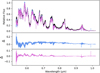 |
Fig. 1 Full spatial summation reduction. Top panel: comparison of Neptune’s visible spectrum before (black), after adjusting for wavelength-dependent centroid shifts (blue), and after the complete targeted spatial extraction (pink). Bottom panels: residuals (Δ). The blue residual shows the difference between the original spectrum and after the centroid shifts (original - centroid shifted). The pink residuals are the difference between the centroid-shifted spectrum and the final version, thus highlighting the stepwise changes (Centroid shifted-final S/N optimized). |
2.4 Instrument response calibration
We calibrated the telescope’s response by comparing the observed spectra of telluric standard stars (white dwarfs LTT7897, Feige110, and GD71) to their high-precision reference spectra provided by ESO. For each observation, we extracted the standard star spectrum using the same procedure described in Sects. 2.2 and 2.3 and then normalized it by exposure time. We then divided the observed flux of our target by the reference spectrum to generate a raw response curve, masking strong telluric absorption regions to avoid errors from residual atmospheric features. We fit this using a fifth-degree polynomial to remove high-frequency noise introduced by observational conditions, resulting in our final response curves. We then applied them to the planetary spectra to correct for instrumental effects and wavelength-dependent instrument sensitivity. Appendix A.4 provides further details on the derivation and application of the response curves.
3 Results
In this section, we present the fully corrected spectra of Uranus, Neptune, Saturn, and Titan (Fig. 2). We also explore their atmospheric compositions by analyzing the absorption features of methane as a case study to exemplify the utility of our dataset.
We compared the methane distribution between Saturn, Uranus, and Neptune using EW measurements. In this analysis, our primary focus was on comparing these results across planets to uncover trends in atmospheric composition and variability. Table 2 contains the measured results, which are discussed in detail in the following subsections. Though not a full atmospheric retrieval study, our analysis is demonstrative the comparative power of our dataset. By examining how methane appears under the different environmental conditions of Saturn and Titan compared to Uranus and Neptune, we provide a framework for understanding the broader implications of planetary formation and evolution in the outer Solar System.
To validate the reliability of our spectra, we compared our reduced data against existing observations from the NASA Infrared Telescope Facility (IRTF) Spectral Library (Sromovsky et al. 2001; Rayner et al. 2003, 2009). The IRTF library provides 0.8-5.0 μm spectra at a resolving power of R ≡ λ/∆λ ~ 2000, obtained with the SpeX medium-resolution spectrograph at Mauna Kea. Figure 3 shows an example of our X-shooter spectrum of Neptune plotted against the corresponding IRTF spectrum. The datasets diverge progressively at longer wavelengths, with our spectrum showing lower flux in the infrared. We attribute this discrepancy to the presence of clouds during our observations, as atmospheric water vapor absorption is particularly strong in this regime. In addition, in the figure we indicate regions affected by strong and moderate telluric absorption, which were not reliably corrected by MOLECFIT and are therefore flagged as less trustworthy.
To investigate methane, we calculated the EWs of a selection of bands. Details of our methods can be found in Appendix B. Figure 4 shows an example of a feature fit, while additional features are numerically stated in Table 2 and visually displayed in Fig. 5. Interpreting these EWs in terms of absolute methane abundance is nontrivial, as an EW depends on the absorber abundance as well as on the scattering by clouds or hazes along the vertical column probed by the observation. For the giant planets, our EW trends are consistent with the broad literature result that states the ice giants exhibit a substantial tropospheric CH4 mixing ratio. Saturn shows a mostly lower mixing ratio in the pressure levels sampled here. We note that differences in cloud structure, viewing geometry, and observing conditions can produce EW differences that do not map uniquely to abundance differences. In particular, ammonia and ammonium-hydrosulfide cloud decks on Saturn can mask gas absorption originating deeper in the atmosphere, reducing measured EWs even when methane is present at depth (Roman et al. 2013). Likewise, poorer observing conditions (for example during the Neptune observation night in comparison to Uranus) can reduce apparent EW and bias comparisons.
Titan’s atmosphere and aerosol and condensate structures differ from those of the giant planets. Surface CH4 can reach several percent by volume, but the thick photochemical haze strongly scatters and attenuates the contribution inhomogeneously. Because of this, we do not infer direct CH4 abundance differences between Titan and the gas or ice giants using EWs. Titan’s strong vertical methane gradient and optically thick haze require radiative-transfer retrievals tailored to Titan’s atmosphere for a reliable abundance estimate (Nixon 2024). Given the degeneracy between the abundance and depth in EW measurements, we therefore compared relative band strengths qualitatively, and we reserve statements concerning quantitative abundance to future work, as they require full radiative-transfer retrievals.
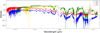 |
Fig. 2 Fully corrected and calibrated albedos of Titan (yellow), Saturn (green), Uranus (blue), and Neptune (red) covering 0.3 μm to 2.1 μm, offset for clarity. Regions of strong telluric absorption are masked in lighter shades, and it should be noted that they are less reliably corrected. The flat regions in the UV were flagged as bad pixels in all images by X-shooter. We also highlight a vertical discontinuity between the VIS and NIR arms of Titan, which is likely due to weather inconsistency. The colors used for these objects are the same in the following figures. |
Equivalent widths.
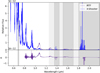 |
Fig. 3 Comparison between our X-shooter spectrum of Neptune (blue) and the corresponding IRTF reference spectrum (purple) with residuals below. Our spectrum shows a systematically lower flux as it progresses into the infrared, which we attribute to the presence of clouds during the observations. Regions of strong (dark gray) and moderate (light gray) telluric absorption are indicated. These regions were not reliably corrected by MOLECFIT and are flagged as less trustworthy. |
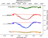 |
Fig. 4 >Methane 0.619 band. The dashed red lines represent the baseline for comparison, while teal lines indicate a Gaussian fit of the absorption feature for visual aid. The black line under the object name on the left shows the calculated EW. |
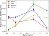 |
Fig. 5 Equivalent width values of the various methane bands. Note that Saturn and Titan trend with each other, as do Uranus and Neptune. |
4 Conclusions
With this work, we have presented a new intermediate-resolution spectral library of outer Solar System bodies acquired using a single instrument, calibration strategy, and reduction pipeline to ensure internal consistency across targets. We demonstrated the power of homogeneous data to support direct, meaningful comparisons between planetary atmospheres through our analysis of Saturn, Uranus, Neptune, and Titan. The resulting dataset is uniquely suited to comparative planetology, bridging the divide between targeted Solar System studies and the broader context of exoplanetary atmospheres.
The uniformity of this dataset enables a level of comparability not achievable with previous compilations, which often suffer from a variety of spectral resolutions, calibrations, and observational geometries. In our case study of methane (CH4), this consistency allowed us to isolate spectral differences attributable to physical and chemical variations in the atmospheres themselves, rather than instrumental or processing artifacts.
We have demonstrated the utility of these data by using them to look into a key question in planetary science. We investigated the differences between the methane abundances of our objects and the implications on atmospheric mixing and transport. We note that the ice giants show lower abundances of methane than Saturn and Titan, indicating that they formed in a cooler environment. We also note that Saturn has the lowest abundance in the visible range, indicating that it has deeper atmospheric methane confinement.
These results also have implications for exoplanet characterization. As next-generation facilities such as the Extremely Large Telescopes, space telescopes such as the James Webb Space Telescope, the Habitable Exoplanet Observatory, and others prepare to probe the atmospheres of cold exoplanets at higher resolutions, Solar System spectra provide vital reference points. The well-characterized and spatially resolved nature of our targets offers an opportunity to test retrieval algorithms, explore chemical degeneracies, and build spectral libraries for planetary classification frameworks.
In making this library publicly available, we aim to support both Solar System researchers and exoplanet modelers alike. Future expansions of this dataset may include additional Solar System bodies, such as Enceladus, Jupiter and its moons, Venus, and Pluto, in order to broaden the comparative scope. Moreover, coupling these spectra with radiative transfer models or retrieval tools will further enhance their scientific value and enable direct interpretation of molecular abundances, thermal profiles, and cloud structures across diverse planetary environments. While full atmospheric retrieval is beyond the scope of this paper, such modeling will be useful for validating this dataset and is planned for future work. Ultimately, this spectral library lays the groundwork for a more unified approach to studying planetary atmospheres that connects Solar System and exoplanet science.
Acknowledgements
We acknowledge the ESO/X-shooter team for their valuable assistance. AB acknowledges support from the Deutsche Forschungsgemeinschaft (DFG, German Research Foundation) under Germany’s Excellence Strategy - EXC 2094 - 390783311. We also would like to acknowledge the referee for their valuable comments and time, which greatly improved the quality of this work.
References
- Atreya, S. K., Crida, A., Guillot, T., et al. 2018, in Saturn in the 21st Century, 1st edn., eds. K. H. Baines, F. M. Flasar, N. Krupp, & T. Stallard (Cambridge University Press), 5 [Google Scholar]
- Atreya, S. K., Hofstadter, M. H., In, J. H., et al. 2020, Space Sci. Rev., 216, 18 [Google Scholar]
- Cassan, A., Kubas, D., Beaulieu, J.-P., et al. 2012, Nature, 481, 167 [NASA ADS] [CrossRef] [Google Scholar]
- Chavez, E., De Pater, I., Redwing, E., et al. 2023, Icarus, 404, 115667 [NASA ADS] [CrossRef] [Google Scholar]
- Coddington, O. M., Richard, E. C., Harber, D., et al. 2023, Earth Space Sci., 10, e2022EA002637 [Google Scholar]
- Fernandes, R. B., Mulders, G. D., Pascucci, I., Mordasini, C., & Emsenhuber, A. 2019, ApJ, 874, 81 [NASA ADS] [CrossRef] [Google Scholar]
- Fink, U., & Larson, H. P. 1979, ApJ, 233, 1021 [NASA ADS] [CrossRef] [Google Scholar]
- Fletcher, L. N., Helled, R., Roussos, E., et al. 2020, Planet. Space Sci., 191, 105030 [NASA ADS] [CrossRef] [Google Scholar]
- Hayes, A. G. 2016, Annu. Rev. Earth Planet. Sci., 44, 57 [Google Scholar]
- Hörst, S. M. 2017, J. Geophys. Res.: Planets, 122, 432 [CrossRef] [Google Scholar]
- Ingersoll, A. P. 2020, Space Sci. Rev., 216, 122 [Google Scholar]
- Kausch, W., Noll, S., Smette, A., et al. 2015, A&A, 576, A78 [NASA ADS] [CrossRef] [EDP Sciences] [Google Scholar]
- Kuiper, G. P. 1944, ApJ, 100, 378 [NASA ADS] [CrossRef] [Google Scholar]
- Lutz, B. L., Owen, T., & Cess, R. D. 1976, ApJ, 203, 541 [Google Scholar]
- Madden, J. H., & Kaltenegger, L. 2018, Astrobiology, 18, 1559 [NASA ADS] [CrossRef] [Google Scholar]
- Modigliani, A., & Bramich, D. 2024, xshoo-pipeline-manual-3.6.8.pdf [Google Scholar]
- Moses, J. I., Fletcher, L. N., Greathouse, T. K., Orton, G. S., & Hue, V. 2018, Icarus, 307, 124 [Google Scholar]
- Moses, J. I., Cavalie, T., Fletcher, L. N., & Roman, M. T. 2020, Philos. Trans. R. Soc. A, 378, 20190477 [Google Scholar]
- Müller-Wodarg, I., Strobel, D., Moses, J., et al. 2008, Space Sci. Rev., 139, 191 [Google Scholar]
- Nelson, R. C., Plyler, E. K., & Benedict, W. S. 1948, J. Res. Natl. Bur. Stan., 41, 615 [Google Scholar]
- Nixon, C. A. 2024, ACS Earth Space Chem., 8, 406 [NASA ADS] [CrossRef] [Google Scholar]
- Payne, A., Villanueva, G. L., Kofman, V., et al. 2025, arXiv e-prints [arXiv:2508.13368] [Google Scholar]
- Rakich, A. 2021, Appl. Sci., 11, 6261 [Google Scholar]
- Rayner, J. T., Toomey, D. W., Onaka, P. M., et al. 2003, PASP, 115, 362 [NASA ADS] [CrossRef] [Google Scholar]
- Rayner, J. T., Cushing, M. C., & Vacca, W. D. 2009, ApJS, 185, 289 [Google Scholar]
- Roe, H. G. 2012, Annu. Rev. Earth Planet. Sci., 40, 355 [Google Scholar]
- Roman, M. T., Banfield, D., & Gierasch, P. J. 2013, Icarus, 225, 93 [Google Scholar]
- Roman, M. T., Fletcher, L. N., Orton, G. S., et al. 2022, Planet. Sci. J., 3, 78 [NASA ADS] [CrossRef] [Google Scholar]
- Smette, A., Sana, H., Noll, S., et al. 2015, A&A, 576, A77 [NASA ADS] [CrossRef] [EDP Sciences] [Google Scholar]
- Sromovsky, L. A., Fry, P. M., Dowling, T. E., Baines, K. H., & Limaye, S. S. 2001, Icarus, 149, 459 [NASA ADS] [CrossRef] [Google Scholar]
- Tollefson, J., de Pater, I., Molter, E. M., 2021, Planet. Sci. J., 2, 105 [Google Scholar]
- Vernet, J., Dekker, H., D’Odorico, S., et al. 2011, A&A, 536, A105 [NASA ADS] [CrossRef] [EDP Sciences] [Google Scholar]
Appendix A Data processing
We provide an overview of the methodology employed in this study, detailing the data acquisition process, spectral analysis techniques, and calibration procedures used to derive the final wavelength-dependent albedos.
Appendix A.1 Data acquisition with X-shooter
Observations were conducted using the Very Large Telescope (VLT) at the Cerro Paranal facility in Chile operated by the European Southern Observatory (ESO). We employed the X-shooter instrument in its Integral Field Unit (IFU) mode, which provides a combined spatial and spectral resolution, hereafter referred to as “spaxels.” The IFU mode covers a spatial field of view of 4” × 1.8” and wavelengths ranging from 0.3 to 2.5 μm. It has a grid of 3 by 26 spaxels, totaling 78. The instrument’s spectral resolution varies across its three arms, with R ≈ 8600 (UVB), R ≈ 13 500 (VIS), and R ≈ 8300 (NIR; Vernet et al. 2011). We selected the IFU mode because it captures spatially resolved spectra, allowing us to probe atmospheric inhomogeneities or surface features across the planets and moons in future work.
Observations were conducted between 2018 and 2021 in service mode under the following program IDs: 0100.C-0473, 0102.C-0481, 0103.C-0460, 105.20J2.001-003, and 108.22EQ.001-002. We prioritized dates when the targets were in opposition to Earth to ensure optimal visibility and minimal atmospheric interference, We also aimed to schedule the observations during periods free and clear of moon transits to avoid contamination (Table 1). Figure A.1 shows an example of the data before cube reconstruction. The acquired data were then processed through ESO’s X-shooter reduction pipeline, which includes steps for bias subtraction, flat-fielding, and wavelength calibration (Modigliani & Bramich 2024). Figure A.2 shows a slice of the cube after the pipeline.
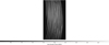 |
Fig. A.1 Raw IFU slice from X-shooter observations the visible range (559.5-1024 nm). The bright horizontal-curved stripes are echelle orders produced by the cross-dispersed echelle spectrograph design. Each stripe corresponds to a different order of the diffraction grating, covering a different wavelength range. The spatial information is along the width of each stripe. This image precedes the X-shooter reduction pipeline and reconstruction of the data cube. |
Appendix A.2 Targeted spatial extraction
Spatial summation was employed as a workaround due to the reconstruction challenges posed by the IFU mode and the lack of support for IFU mode in MOLECFIT (described in greater detail in Appendix A.3). In this first paper, we collapsed the IFU into a single spectrum. Rather than using the spectrum from every pixel, we integrated only the flux values from within the disk of the observed object. For the spatial extraction, we used the approach detailed in this section to select the best pixels and sum the flux over the spatial extent, leading to more accurate representations of the observed bodies’ atmospheres. The IFU field of view was sufficient to capture the full disk of Titan within a single exposure. Uranus and Neptune, while still relatively compact, each required two adjacent pointings to achieve full-disk coverage. In the case of Saturn whose angular extent far exceeds the IFU field, complete mapping was not feasible within the scope of this program. Instead, we obtained a small mosaic sampling both the vertical and horizontal extents of the disk. For consistency with the rest of the dataset, only exposures free from significant contamination by Saturn’s rings were retained. A total of eleven such exposures were selected and summed for the final spectrum. A map of the acquired images for Saturn is displayed in Fig. A.3.
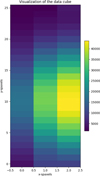 |
Fig. A.2 Processed slice of the Neptune IFU data after passing through the ESO reduction pipeline. In addition to the reconstruction of the data cube, the pipeline includes initial processing stages such as bias subtraction, flat-fielding, and wavelength calibration. In this instance, the IFU covered one-half of the planet Neptune in the spatial directions, indicated here in photons. |
Atmospheric dispersion, which results from the differential refraction of light at different wavelengths as it passes through Earth’s atmosphere, can cause misalignment in spectral space, especially in the absence of Atmospheric Dispersion Correctors (ADCs) in X-shooter’s IFU mode (Rakich 2021). To correct for this, we tracked the object’s center of mass for each wavelength slice in both the x- and y-directions. We then fit parabolic curves to the center positions in both directions as a function of wavelength, correcting for the dispersion by shifting the data cube accordingly. This method ensured the proper alignment of spectral features across the wavelength range and is visualized in Fig. A.4. The results of the dispersion correction are shown in Fig. A.5.
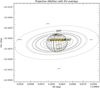 |
Fig. A.3 X-shooter IFU mosaic over a wireframe of Saturn. Each rectangular footprint represents a single IFU pointing overlaid on a schematic projection of Saturn and its rings. Observations sample both latitudinal and longitudinal sections of the planetary disk. Eleven exposures were selected for the final spectrum, chosen to avoid contamination from Saturn’s ring system, while the remainder of the offsets have been grayed out. The orientation and coverage reflect the IFU’s 4″×1.8″ field of view. Several of Saturn’s inner moons are labeled for reference. |
Sigma clipping was employed to remove spurious data points caused by cosmic rays, detector noise, or other transient effects. We calculated the median flux for each pixel using a window of neighboring wavelength slices for each wavelength slice. The interquartile range (IQR) was then calculated from the deviation of the pixel’s flux from the median value. Any pixel whose deviation exceeded a specified significance threshold was considered an outlier. These outliers were then replaced by the median value for that pixel within the wavelength plane. This approach effectively mitigates anomalous data points, improving the reliability of the final spectrum. The results of this step are shown in Fig. A.6.
To select the optimal radius for spatial integration, we calculated the distance of each pixel from the center of the object and summed the flux for all pixels within increasing radii. In the case of Saturn, the object "center" was determined as the brightest pixels in each image. For each radius, the signal was computed as the sum of flux across all included pixels, while the noise was determined from the standard deviation of the residuals after fitting a linear model to the summed flux across the wavelength range. The S/N was calculated for each radius, and we fit a theoretical model assuming that S/N increases with the square root of the signal. The optimal radius was defined as the point where the actual S/N deviated from the theoretical model by more than a specified error threshold of 20%. This ensures that the selected radius includes the maximum useful flux while avoiding unnecessary systematic noise from background regions. An example is shown in Fig. A.7, with the signal as a function of radius in Fig. A.8.
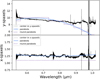 |
Fig. A.4 Movement of the central pixel in both x- and y-directions for the observed object, Neptune, across the full wavelength range. This process ensures the proper alignment of spectral features for the spatial summation process. |
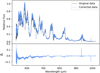 |
Fig. A.5 Comparison of Neptune spectrum before (black) and after (blue) applying atmospheric dispersion correction (top) and the residuals between the two (bottom). This correction realigns spectral features that were misaligned due to differential atmospheric refraction. |
Following these corrections, we finally summed the flux of each pixel that fell within the radius to compute the total flux at each wavelength. This flux should then accurately represent the contribution from the spatial extent of the images while minimizing contamination from background noise or unrelated areas of the field of view. The result of the spatial integration was a one-dimensional spectrum representing the integrated flux of all selected spaxels as a function of wavelength. The integrated flux was then used in subsequent analysis. A comparison of the spectrum before and after the full integration process is displayed in Fig. A.9.
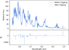 |
Fig. A.6 Impact of sigma clipping on spectrum quality. Neptune spectrum shown before (black) and after (blue) applying sigma clipping, a technique that removes outliers caused by cosmic rays or detector noise, resulting in cleaner data (top). The residuals between the two are in the bottom panel. |
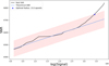 |
Fig. A.7 Optimal radius selection for spatial integration. This visualizes how the S/N deviates from the theoretical S/N model as the integration radius increases. The selected optimal radius includes maximum useful flux while minimizing background noise, leading to more accurate integrated spectra. |
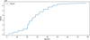 |
Fig. A.8 Variation in the signal with the spaxel count. The signal does not increase linearly with the addition of more pixels, but follows this step-wise pattern. |
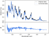 |
Fig. A.9 Neptune’s spectrum before (black) and after (blue) the full spatial integration (top). The rescaled blue spectrum represents the summed flux from all pixels within the spatial integration region, providing a more complete spectral signature of the planet. The residuals between the two are shown on bottom. |
Appendix A.3 Removal of telluric absorptions
Ground-based astronomical observations are inevitably affected by telluric absorption, where molecules in Earth’s atmosphere—such as water vapor, oxygen, and carbon dioxide—introduce spectral features that overlap with those of celestial objects. These telluric lines, particularly prominent in the near-infrared, can obscure or distort the intrinsic spectra of planetary atmospheres, stars, and other astronomical sources. To accurately interpret the data, it is important to remove these atmospheric contributions.
In this work, we used MOLECFIT (Smette et al. 2015; Kausch et al. 2015) to model and remove telluric absorption features from the spectra of our observed Solar System bodies. MOLECFIT fits a detailed atmospheric model to the observed spectrum and the specific atmospheric conditions at the time of observation. MOLECFIT generates a synthetic telluric spectrum that closely matches the observed telluric lines by adjusting parameters such as airmass, temperature, and water vapor content. The software then removes these lines from the data, either by dividing or subtracting the modeled spectrum, depending on the nature of the contamination. An example of the results of this are shown in Fig A.10.
While MOLECFIT is a powerful tool for telluric correction, it was not initially designed to handle the unique format of X-shooter’s IFU data in its native state. MOLECFIT’s algorithms are optimized for long-slit and point-source spectra, and its mostly automatic processing workflow encountered difficulties with our IFU data, recognizing it as incorrectly formatted and refusing to proceed with the telluric correction. To overcome this issue we implemented a workaround that required custom adjusting of MOLECFIT internal files and several headers of our collected collapsed spectrum.
While powerful, MOLECFIT often amplifies noise in regions of intrinsically low flux. In deep atmospheric absorption bands, the observed spectrum approaches zero, meaning that even minimal mismatches between the data and the modeled transmission can produce large relative artifacts in the corrected spectrum. These manifest as narrow spikes or inverted features that were not visible in the original data. To address this, we classified each wavelength region into three categories: trustworthy, use with caution, and untrustworthy, based on the strength of atmospheric absorption and the fit quality reported by MOLECFIT. These masks are distributed with the final spectra in the FITS headers, allowing users to easily identify and exclude or down-weight unreliable portions of the data during subsequent analyses.
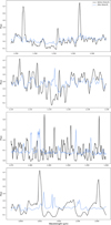 |
Fig. A.10 Comparison of MOLECFIT results. These are a selection of water features in different regions of the NIR range, the most difficult to correct. The blue line shows how MOLECFIT has performed in correcting these features. |
Appendix A.4 Telescope response curve
The telescope response curve is a function that describes how the instrument (telescope, optics, and detectors) responds to incoming light across different wavelengths. Every instrument introduces distortions and variations in how it records light due to factors such as mirror reflectivity, filter transmission, detector efficiency, and atmospheric effects. These distortions cause the raw data to differ from the true physical values. We correct for these distortions by quantifying the instrument’s sensitivity at each wavelength, resulting in the response curve. Applying the response curve to observed spectra can normalize the data and remove instrumental biases, enabling direct comparisons between observations and theoretical models.
In this work, we created the telescope response curves by characterizing the instrument’s sensitivity across X-shooter’s ultraviolet, visible, and near-infrared arms individually. We derived response curves by comparing the observed spectra of telluric standard stars with their known reference spectra provided by ESO.
For each observation, a telluric standard star was chosen based on the observed object. We used LTT7897, Feige110, or GD71 as telluric standards, depending on the object’s position in the sky, and obtained images on the same nights as our planetary spectra in IFU mode as well. After processing the flux data for each in the same way as our planetary spectra, we normalized the data by dividing by the exposure time and scaling it by the 99th percentile of the flux values to correct for instrument sensitivity. By using the 99th percentile, we avoided the regions of extreme flux at the edges of the spectral arms.
To avoid regions of telluric absorption, we masked any area of the spectra that was significantly affected by atmospheric absorption features, such as those dominated by water vapor and oxygen. This ensured that only the reliable portions of the spectra were used for this calibration. We extracted the corresponding sections of the reference spectrum for the UVB, VIS, and NIR arms and applied a linear scaling to the full spectrum to match the observed data. By comparing the observed flux to the reference flux, we constructed wavelength-dependent response curves for each observation. These curves were then used to correct the science spectra, ensuring accurate flux measurements for subsequent analysis. Our resulting curves are shown in Fig A.11.
For many nights, the standard star was not observed immediately before or after our target. Because of this, the weather changed between observations, leading to differences in the telluric corrections between the standard stars and the targets. This resulted in an imperfect match between the UVB, VIS, and NIR bands at this point in our processing. To adjust for this consistently, we matched both the UVB and NIR bands to the VIS using a polynomial fit at the edges and scaled the spectrum accordingly.
Appendix A.5 Solar spectrum correction
In order to isolate planetary features from the reflected solar spectrum, we ensure that only the intrinsic spectral features of the observed bodies remain, enabling accurate analysis of atmospheric composition, surface properties, and other physical characteristics.
We sourced the solar spectrum from the University of Colorado’s Laboratory for Atmospheric and Space Physics (LASP)’s online catalog: LISIRD (Coddington et al. 2023). We opted to use the LISIRD solar spectrum rather than the standard solar twin stars observed on the same night due to the higher resolution, absolute irradiance calibration, and spectral stability of the LISIRD dataset. The TSIS-1 HSRS data are free from temporal variability and provide a reliable solar spectrum across the ultraviolet to near-infrared wavelength range.
Their TSIS-1 High Spectral Resolution Spectrometer (HSRS) dataset provides a highly detailed record of solar spectral irradiance (SSI) across the ultraviolet, visible, and nearinfrared regions (Fig A.12). Collected by the Total and Spectral Solar Irradiance Sensor (TSIS-1) aboard the International Space Station (ISS), this dataset offers 1-nm resolution measurements from approximately 200 nm to 2400 nm, comparable to that of X-shooter. The TSIS-1 HSRS data are calibrated to deliver absolute irradiance values with a high degree of accuracy, featuring spectral stability and minimal noise.
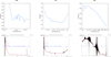 |
Fig. A.11 Response curve results. This figure shows our computed telescope response curves for Neptune for the three arms of X-shooter. Note the residuals left by the standard star in the UVB arm, which were masked to preserve accuracy. These can be compared with those provided on the ESO website, which are shown on bottom. |
Appendix A.5.1 Doppler shift correction
Before removing the solar lines, we used the solar absorption features and the LISIRD spectrum to correct for Doppler shifts induced by the relative motion between the telescope and the target bodies. With this step, we aimed to ensure accurate wavelength calibration for internal consistency within our dataset and comparison with other astronomical data.
We chose a selection of solar absorption features that were both strong and clear to calculate the shift from. For each selected solar absorption feature, we first identified the wavelength corresponding to the minimum flux value in the LISIRD spectrum and our observed data. We defined a narrow search range around each target feature and used Gaussian fitting to refine the location of each absorption feature’s central wavelength. Figure A.13 shows an example of this alignment.
We next performed a linear regression between the observed absorption features and those in the LISIRD reference spectrum to ensure accurate wavelength alignment across the entire spectral range (Fig A.14). This regression corrected for systematic shifts and provided the final radial velocity (RV) correction. The RV was computed based on the relative wavelength shifts between the observed and reference features we corrected each object individually by band.
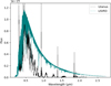 |
Fig. A.12 Solar spectrum correction. The LISIRD solar spectrum (teal) plotted against our observed Uranus data (black). The two spectra are aligned to remove solar reflection, ensuring only intrinsic planetary features are analyzed. |
Appendix A.5.2 Line removal
After correcting for Doppler shifts and aligning the observed wavelengths with the LISIRD spectrum, we proceeded to remove the solar lines from our spectra. The LISIRD solar spectrum has a much higher resolution than our observed data. To match the resolution of our spectra and accurately remove the solar lines, we applied a Gaussian convolution to the solar spectrum. This process smooths the solar spectrum to better correspond with the lower resolution of the observed data, allowing for more effective line removal.
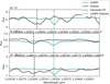 |
Fig. A.13 LISIRD feature comparison with Uranus data. A detailed comparison of a solar absorption feature in the LISIRD spectrum (teal) and the same feature in Uranus’s spectrum (black). The dashed lines mark the feature centers identified by Gaussian fitting for realignment. |
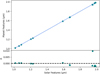 |
Fig. A.14 Radial velocity correction. This displays the location of solar absorption features in our data plotted against the same features in the LISIRD solar spectrum (top). The resulting slope from the linear regression provides the radial velocity correction. The bottom panel shows the residuals. |
To determine the most appropriate Gaussian kernel for the smoothing, we varied the kernel’s size and sigma parameters and evaluated their fitness based on the mean squared error (MSE) between the smoothed reference spectrum and the observed data. For each selected absorption feature, we defined subsets of wavelength and flux arrays based on a 0.04 μm threshold and used the truncated Newton (TNC) minimization method to optimize kernel parameters. The final kernel parameters were computed as the mean size and median sigma across all features. The convolution results are in Fig A.15.
After applying the Gaussian kernel, we interpolated both the smoothed solar and LISIRD spectra using a linear interpolation function to align the wavelength grids with our observed data. The resulting interpolated spectrum was then evaluated against the corrected radial velocity wavelength array.
Once the smoothed and interpolated spectra were aligned with the observed data, we divided the observed flux by the smoothed LISIRD flux to remove the solar line contributions.
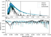 |
Fig. A.15 Convolution results for solar line smoothing. This shows a comparison of the original LISIRD solar spectrum (teal), the smoothed version (blue), and our Uranus data (black). Gaussian convolution was applied to smooth the high-resolution LISIRD spectrum to match the resolution of our data, improving line removal efficiency. |
This produced a clean, corrected albedo, which was then saved for analysis (Fig A.16).
Appendix B Equivalent widths
Equivalent widths are one way to measure the significance of a spectral feature with common indexes being used to directly compare molecular abundances between datasets. Here, we provide a detailed explanation of how we calculated and verified them in this work.
First, we fit the continuum by excluding the absorption feature between wavelengths λ1 and λ2, modeling the remaining spectrum with a linear polynomial. The coefficients a and b are determined via a least-squares minimization of the residuals between the observed flux values Fi and the model C(λi) at each continuum point. This is equivalent to minimizing:
![Mathematical equation: S(a, b) = \sum_{i=1}^{N} \left[ F_i - (a \lambda_i + b) \right]^2.](/articles/aa/full_html/2026/03/aa55769-25/aa55769-25-eq1.png) (B.1)
(B.1)
The resulting optimal parameters are
 (B.2)
(B.2)
 (B.3)
(B.3)
where the summations run over the N continuum data points outside the absorption region. Next, we calculate the area of the absorption feature between the fitted continuum and the observed flux:
![Mathematical equation: A = \int_{\lambda_1}^{\lambda_2} \left[ C(\lambda) - F(\lambda) \right] d\lambda,](/articles/aa/full_html/2026/03/aa55769-25/aa55769-25-eq4.png) (B.4)
(B.4)
where F(λ) is the observed flux. The EW is then computed by normalizing this area by the mean continuum level over the absorption region:
 (B.5)
(B.5)
where C is the mean value of the fitted continuum within λ1 ≤ λ ≤ λ2:
 (B.6)
(B.6)
Finally, the uncertainty in the EW is propagated via
 (B.7)
(B.7)
where σA is the uncertainty in the area under the absorption feature, and σC is the standard deviation of the residuals between the continuum fit and the data outside the absorption region. For additional visual validation, we computed Gaussian models for each band but did not use them for the EW calculation.
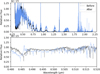 |
Fig. A.16 Correction results for solar contamination. A comparison of the original Uranus data (black) and the results (blue) after the complete process of Doppler shift correction and line mitigation. |
Appendix B.1 Mask creation
These data are presented with two quality masks. The highest level mask marks the regions of highest telluric absorption, where the MOLECFIT model struggles to recover the object’s signal. To do this, we took the difference between a given spectrum immediately before and immediately after the MOLECFIT correction. In regions free of strong telluric absorption, these residuals are expected to be dominated by noise, whereas telluric features manifest as high-amplitude structures.
The telluric mask construction proceeds in two complementary stages. First, a set of known atmospheric absorption bands is defined based on standard telluric features. All wavelengths falling within these predefined intervals are flagged for all objects. To account for variability in line widths and imperfect wavelength alignment, the mask is then adaptively expanded outward from each band edge. This expansion continues until the squared residuals fall below a threshold set by the local noise floor, or until a maximum distance is reached. This step ensures that extended wings of telluric features are consistently captured.
An additional statistical masking step is applied to capture residual outliers not fully encompassed by the predefined bands. A smooth baseline is removed from the residual spectrum using a wide median filter, and the detrended residuals are subjected to an iterative sigma-clipping procedure based on robust median and MAD estimates. Pixels identified as significant outliers are flagged only if they coincide with regions of elevated uncertainty, as indicated by the upper percentile of the propagated error spectrum. These are noted artifacts caused by imperfect correction and this constraint prevents isolated noise spikes in otherwise clean regions from being incorrectly masked. The final telluric mask is constructed as the union of the predefined band mask, the adaptively expanded regions, and statistically significant outliers associated with high uncertainty.
A secondary mask is included with the data products to indicate statistically significant residual features not fully captured by the initial telluric band definitions. To characterize the local statistical behavior of the residuals, we compute a sliding median and median absolute deviation (MAD) over a small wavelength range (151 pixel). A normalized deviation metric is then defined as
 (B.8)
(B.8)
where R̃(λ) denotes the local median of the residuals. The multiplicative factor of 1.4826 rescales the MAD to be a consistent estimator of the standard deviation under the assumption of an underlying Gaussian distribution. Pixels for which the normalized deviation exceeds a threshold of z > 5 are flagged as anomalous, corresponding to deviations beyond the expected local scatter. The resulting mask is then combined with the telluric mask for ease of use. Although the residual distribution in telluric regions is not strictly Gaussian, this scaling provides a stable and conservative measure of statistical significance that is well-suited for identifying coherent deviations associated with atmospheric absorption, without being overly sensitive to noise.
All Tables
All Figures
|
Fig. 1 Full spatial summation reduction. Top panel: comparison of Neptune’s visible spectrum before (black), after adjusting for wavelength-dependent centroid shifts (blue), and after the complete targeted spatial extraction (pink). Bottom panels: residuals (Δ). The blue residual shows the difference between the original spectrum and after the centroid shifts (original - centroid shifted). The pink residuals are the difference between the centroid-shifted spectrum and the final version, thus highlighting the stepwise changes (Centroid shifted-final S/N optimized). |
| In the text | |
|
Fig. 2 Fully corrected and calibrated albedos of Titan (yellow), Saturn (green), Uranus (blue), and Neptune (red) covering 0.3 μm to 2.1 μm, offset for clarity. Regions of strong telluric absorption are masked in lighter shades, and it should be noted that they are less reliably corrected. The flat regions in the UV were flagged as bad pixels in all images by X-shooter. We also highlight a vertical discontinuity between the VIS and NIR arms of Titan, which is likely due to weather inconsistency. The colors used for these objects are the same in the following figures. |
| In the text | |
|
Fig. 3 Comparison between our X-shooter spectrum of Neptune (blue) and the corresponding IRTF reference spectrum (purple) with residuals below. Our spectrum shows a systematically lower flux as it progresses into the infrared, which we attribute to the presence of clouds during the observations. Regions of strong (dark gray) and moderate (light gray) telluric absorption are indicated. These regions were not reliably corrected by MOLECFIT and are flagged as less trustworthy. |
| In the text | |
|
Fig. 4 >Methane 0.619 band. The dashed red lines represent the baseline for comparison, while teal lines indicate a Gaussian fit of the absorption feature for visual aid. The black line under the object name on the left shows the calculated EW. |
| In the text | |
|
Fig. 5 Equivalent width values of the various methane bands. Note that Saturn and Titan trend with each other, as do Uranus and Neptune. |
| In the text | |
|
Fig. A.1 Raw IFU slice from X-shooter observations the visible range (559.5-1024 nm). The bright horizontal-curved stripes are echelle orders produced by the cross-dispersed echelle spectrograph design. Each stripe corresponds to a different order of the diffraction grating, covering a different wavelength range. The spatial information is along the width of each stripe. This image precedes the X-shooter reduction pipeline and reconstruction of the data cube. |
| In the text | |
|
Fig. A.2 Processed slice of the Neptune IFU data after passing through the ESO reduction pipeline. In addition to the reconstruction of the data cube, the pipeline includes initial processing stages such as bias subtraction, flat-fielding, and wavelength calibration. In this instance, the IFU covered one-half of the planet Neptune in the spatial directions, indicated here in photons. |
| In the text | |
|
Fig. A.3 X-shooter IFU mosaic over a wireframe of Saturn. Each rectangular footprint represents a single IFU pointing overlaid on a schematic projection of Saturn and its rings. Observations sample both latitudinal and longitudinal sections of the planetary disk. Eleven exposures were selected for the final spectrum, chosen to avoid contamination from Saturn’s ring system, while the remainder of the offsets have been grayed out. The orientation and coverage reflect the IFU’s 4″×1.8″ field of view. Several of Saturn’s inner moons are labeled for reference. |
| In the text | |
|
Fig. A.4 Movement of the central pixel in both x- and y-directions for the observed object, Neptune, across the full wavelength range. This process ensures the proper alignment of spectral features for the spatial summation process. |
| In the text | |
|
Fig. A.5 Comparison of Neptune spectrum before (black) and after (blue) applying atmospheric dispersion correction (top) and the residuals between the two (bottom). This correction realigns spectral features that were misaligned due to differential atmospheric refraction. |
| In the text | |
|
Fig. A.6 Impact of sigma clipping on spectrum quality. Neptune spectrum shown before (black) and after (blue) applying sigma clipping, a technique that removes outliers caused by cosmic rays or detector noise, resulting in cleaner data (top). The residuals between the two are in the bottom panel. |
| In the text | |
|
Fig. A.7 Optimal radius selection for spatial integration. This visualizes how the S/N deviates from the theoretical S/N model as the integration radius increases. The selected optimal radius includes maximum useful flux while minimizing background noise, leading to more accurate integrated spectra. |
| In the text | |
|
Fig. A.8 Variation in the signal with the spaxel count. The signal does not increase linearly with the addition of more pixels, but follows this step-wise pattern. |
| In the text | |
|
Fig. A.9 Neptune’s spectrum before (black) and after (blue) the full spatial integration (top). The rescaled blue spectrum represents the summed flux from all pixels within the spatial integration region, providing a more complete spectral signature of the planet. The residuals between the two are shown on bottom. |
| In the text | |
|
Fig. A.10 Comparison of MOLECFIT results. These are a selection of water features in different regions of the NIR range, the most difficult to correct. The blue line shows how MOLECFIT has performed in correcting these features. |
| In the text | |
|
Fig. A.11 Response curve results. This figure shows our computed telescope response curves for Neptune for the three arms of X-shooter. Note the residuals left by the standard star in the UVB arm, which were masked to preserve accuracy. These can be compared with those provided on the ESO website, which are shown on bottom. |
| In the text | |
|
Fig. A.12 Solar spectrum correction. The LISIRD solar spectrum (teal) plotted against our observed Uranus data (black). The two spectra are aligned to remove solar reflection, ensuring only intrinsic planetary features are analyzed. |
| In the text | |
|
Fig. A.13 LISIRD feature comparison with Uranus data. A detailed comparison of a solar absorption feature in the LISIRD spectrum (teal) and the same feature in Uranus’s spectrum (black). The dashed lines mark the feature centers identified by Gaussian fitting for realignment. |
| In the text | |
|
Fig. A.14 Radial velocity correction. This displays the location of solar absorption features in our data plotted against the same features in the LISIRD solar spectrum (top). The resulting slope from the linear regression provides the radial velocity correction. The bottom panel shows the residuals. |
| In the text | |
|
Fig. A.15 Convolution results for solar line smoothing. This shows a comparison of the original LISIRD solar spectrum (teal), the smoothed version (blue), and our Uranus data (black). Gaussian convolution was applied to smooth the high-resolution LISIRD spectrum to match the resolution of our data, improving line removal efficiency. |
| In the text | |
|
Fig. A.16 Correction results for solar contamination. A comparison of the original Uranus data (black) and the results (blue) after the complete process of Doppler shift correction and line mitigation. |
| In the text | |
Current usage metrics show cumulative count of Article Views (full-text article views including HTML views, PDF and ePub downloads, according to the available data) and Abstracts Views on Vision4Press platform.
Data correspond to usage on the plateform after 2015. The current usage metrics is available 48-96 hours after online publication and is updated daily on week days.
Initial download of the metrics may take a while.