| Issue |
A&A
Volume 707, March 2026
|
|
|---|---|---|
| Article Number | A13 | |
| Number of page(s) | 15 | |
| Section | Extragalactic astronomy | |
| DOI | https://doi.org/10.1051/0004-6361/202556138 | |
| Published online | 25 February 2026 | |
Tracing ionized gas kinematics in Lyman-break Analogs
Implications for star formation compactness and outflow properties
1
Departamento de Astronomía, Universidad de La Serena Av. Juan Cisternas 1200 Norte La Serena, Chile
2
Instituto de Astrofísica de Andalucía (CSIC) Apartado 3004 18080 Granada, Spain
3
Centro de Estudios de Física del Cosmos de Aragón (CEFCA), Unidad Asociada al CSIC Plaza San Juan 1 E–44001 Teruel, Spain
4
INAF – Osservatorio Astronomico di Roma Via di Frascati 33 00078 Monte Porzio Catone, Italy
5
Michigan Institute for Data Science, University of Michigan 500 Church Street Ann Arbor MI 48109, USA
6
Space Telescope Science Institute 3700 San Martin Drive Baltimore MD 21218, USA
★ Corresponding authors: This email address is being protected from spambots. You need JavaScript enabled to view it.
; This email address is being protected from spambots. You need JavaScript enabled to view it.
Received:
27
June
2025
Accepted:
12
November
2025
Abstract
Context. The ionized gas kinematics of low-mass starburst galaxies is a tracer of galaxy interactions and feedback processes, which are key for understanding massive star formation, chemical enrichment, and galaxy evolution.
Aims. We studied the ionized gas kinematics and outflow properties of a sample of Lyman-break analogs (LBAs) at z ∼ 0.1 − 0.3; these LBAs are characterized by compact morphologies, high UV luminosities, and strong emission lines, which are common at higher redshifts.
Methods. We used high-resolution VLT/X-shooter spectra of 14 compact, UV-luminous LBAs to model the complex [O III]λλ4959,5007 Å and Balmer line profiles with multi-Gaussian fits.
Results. The kinematics of LBAs are complex, with emission lines best reproduced by narrow (σ < 90 km s−1) and broad (σ > 90 km s−1) components in all galaxies. The narrow-line kinematics is highly turbulent, likely driven by massive star-forming clumps. The luminosities and line ratios of the narrow components are typical of giant H II regions. We interpret the broader components as ionized outflows driven by strong winds of massive stars and supernovae. In galaxies with highly complex profiles and disturbed morphologies, ongoing interactions or mergers are found to contribute to the broad components. We find outflow velocities (vout) in the range ∼200 km s−1 to 500 km s−1. Simple models yield outflow mass rates of 0.20–2.72 M⊙ yr−1 and mass-loading factors (η) of ∼0.03–0.81. We find that η shows a mild increasing trend at lower stellar masses, in agreement with previous observational studies and predictions from FIRE-2 and Illustris-TNG simulations. Compact starburst morphologies can modulate the η-M★ relation, which is strongly correlated as ΣSFR-η, i.e., more compact starbursts drive stronger outflows. We find a good agreement with similar findings in star-forming galaxies at high redshifts (z ∼ 2 − 9), including those from recent JWST observations.
Conclusions. Our results highlight the relevance of detailed studies of the ionized gas kinematics in local UV-compact starbursts to improve our understanding of feedback processes in low-mass, rapidly star-forming galaxies.
Key words: galaxies: ISM / galaxies: kinematics and dynamics / galaxies: starburst
© The Authors 2026
 Open Access article, published by EDP Sciences, under the terms of the Creative Commons Attribution License (https://creativecommons.org/licenses/by/4.0), which permits unrestricted use, distribution, and reproduction in any medium, provided the original work is properly cited.
This article is published in open access under the Subscribe to Open model. This email address is being protected from spambots. You need JavaScript enabled to view it. to support open access publication.
1. Introduction
Understanding feedback from stellar winds, supernovae (SNe), and active galactic nuclei (AGNs), and its impact on the interstellar medium (ISM), is crucial to quantifying the escape of ionizing photons at the epoch of reionization (z ≳ 6; Robertson et al. 2015) and the baryon cycle that regulates galaxy growth and chemical evolution over cosmic time (Tumlinson et al. 2017). Feedback from star formation and AGN activity, together with mass and environment, is a primary driver of star-formation quenching (Peng et al. 2010; Sawala et al. 2016). Low-mass galaxies, with shallow potential wells, experience stronger feedback effects (Muratov et al. 2015). However, the impact of stellar feedback and outflows on metal enrichment and ionizing-photon escape remains uncertain in the youngest high-z galaxies (Llerena et al. 2023; Carniani et al. 2024; de Graaff et al. 2024; Rodríguez Del Pino et al. 2024; Saldana-Lopez et al. 2025; Cooper et al. 2025).
Lyman-break galaxies (LBGs) are the most common population of UV-luminous star-forming galaxies at redshifts (z) ≳2, largely contributing to both the galaxy number densities and the global star-formation rate (SFR) density at these epochs (e.g., Bouwens et al. 2021). Thus, they are typically identified as dropouts in deep photometric surveys by their bright and blue UV continuum with a strong depression near the Lyman limit (e.g., Giavalisco 2002, and references therein) and later confirmed with deep spectroscopy (e.g., Shapley et al. 2003; Le Fèvre et al. 2015; Pentericci et al. 2018). Bright LBGs typically exhibit stellar masses between 109 and 1010 M⊙, SFRs ranging from 10 to 100 M⊙ yr−1 (Shapley et al. 2001; Steidel et al. 1996; Giavalisco 2002), and subsolar metallicities (e.g., Maiolino et al. 2008; Cullen et al. 2019). More recent JWST observations have detected fainter LBGs with lower stellar masses at the highest redshifts (Finkelstein et al. 2024; Arrabal Haro et al. 2023; Bunker et al. 2024). However, because of their relative faintness and high redshifts, the ionized gas kinematics and outflow properties of LBGs remain challenging to study.
Local analogs of high-z LBGs offer a way to study feedback and outflows under comparable ISM conditions. Complementing UV-based studies with optical kinematics provides a more thorough picture of these galaxies. While UV absorption lines trace extended and diffuse gas on large scales, the study of ionized gas through optical emission lines provides insights into denser gas closer to regions of active star formation (e.g., Xu et al. 2022, 2025a; Martin et al. 2024). A key local analog sample is the Lyman-break analogs (LBAs; Heckman et al. 2005; Hoopes et al. 2007) at z of ∼0.1–0.3, defined by high far-UV (FUV) luminosities (LFUV > 2 × 10¹⁰ L⊙) and surface brightnesses (IFUV > 109 L⊙ kpc−2). Their multiwavelength properties, morphologies, stellar and ISM characteristics, radio/X-ray emission, and environments have been widely studied, reinforcing their analogy with high-z galaxies. (Overzier et al. 2008, 2009; Basu-Zych et al. 2009a,b, 2013; Gonçalves et al. 2014; Contursi et al. 2017; Loaiza-Agudelo et al. 2020; Santana-Silva et al. 2020; Santos-Junior et al. 2025; Araujo-Carvalho et al. 2025). Overall, they are relatively low-mass systems (M★ ∼ 109.5–1011 M⊙) with high SFRs (∼10–100 M⊙ yr−1) and span a wide range of morphologies, with many showing evidence of interactions or merging. They also span a wide range of metallicities and ionization properties, with some of their characteristics overlapping with other local analogs, such as the Green Pea galaxies (e.g., Amorín et al. 2010, 2012a; Brown et al. 2014; Loaiza-Agudelo et al. 2020).
The kinematic and feedback properties of LBAs have been studied using mostly UV absorption lines (Heckman et al. 2011). Heckman et al. (2015) analyzed galactic winds for a large sample of 39 LBAs using Hubble Space Telescope (HST) Cosmic Origins Spectrograph (COS) and Far Ultraviolet Spectroscopic Explorer (FUSE) observations and found that the outflow velocity correlates weakly with the stellar mass but strongly with the SFR and the SFR surface density. This suggests that concentrated star formation in UV-luminous galaxies drives stronger outflows. Heckman & Borthakur (2016) extended this analysis to extreme starburst galaxies, confirming previous relations between outflow velocity (Vout) and variables such as stellar mass and the SFR. Their findings suggest that outflows consist of interstellar or circumgalactic clouds accelerated by a combination of gravitational forces and the momentum of the outflows. An important conclusion from these studies is that such extreme feedback could be required to create channels or holes that enable the escape of ionizing radiation from star-forming galaxies (Heckman et al. 2011; Borthakur et al. 2014; Alexandroff et al. 2015). These UV-based studies mainly trace extended, diffuse gas on galactic scales.
On the other hand, only a few studies have examined the ionized gas kinematics of LBAs through spectroscopic observations. Overzier et al. (2009) analyzed high-resolution spectra of four LBAs with strong signatures of AGN activity, and Gonçalves et al. (2010) presented the first spatially resolved study of a larger sample of LBAs using adaptive-optics-assisted near-infrared (NIR) integral field spectroscopy. The authors examined the most compact emission line regions of LBAs; they found a relatively large velocity dispersion, which suggests strong turbulence in the ionized gas. However, in the star-forming LBAs, they found no clear evidence of outflows, possibly due to the limited depth of such observations. Only for a few LBAs, also classified as Green Pea galaxies, did Amorín et al. (2012b) present evidence of complex gas kinematics and ionized outflows using high-dispersion spectra. Similarly, Hogarth et al. (2020) studied the ionized gas kinematics of one of the most compact LBAs using echelle optical spectra, finding strong signatures of photoionized outflowing gas in the form of broad emission components in both Balmer and collisionally excited lines, similar to other local analogs (Bosch et al. 2019; Amorín et al. 2024). These authors studied the physical properties and metallicity of the outflow component, finding evidence of relative enrichment due to the gas dispersed by the outflow and highlighting the role of feedback in clearing holes and channels in the ISM through which ionizing photons could escape.
Building on previous work, we analyzed ionized-gas kinematics in 14 LBAs using high-dispersion optical spectroscopy, providing new insight into their outflow properties and feedback impact. These results provide a benchmark for detailed comparisons with high-redshift LBGs.
The paper is structured as follows. Section 2 describes the LBA sample and spectroscopic data, Sect. 3 the line-fitting methodology, and Sect. 4 the results. We discuss our results in Sect. 5 and provide our conclusions in Sect. 6. Throughout this work, we assume a standard cosmological model with a Hubble constant (H0) of 70 km s−1 Mpc−1, a matter density parameter (ΩM) of 0.3, and a vacuum energy density parameter (ΩΛ) of 0.7.
2. Galaxy sample and data
Our sample comprises 14 LBAs, which are part of the 30 galaxies with Very Large Telescope (VLT) X-shooter spectroscopy presented in the work of Loaiza-Agudelo et al. (2020) focused on emission-line diagnostics and chemical abundances. That sample belongs to a parent sample of 74 LBAs, selected by Heckman et al. (2005) and studied in detail by Overzier et al. (2009).
The selected LBAs are relatively low-mass and compact, with stellar masses M★ ∼ 109.3 − 1010.7 M⊙ (median 109.9 M⊙) and optical effective radii 0.77–4.6 kpc (median 1.75 kpc) from HST F606W/F850LP imaging Overzier et al. (2009). Selection follows the FUV-luminosity and compactness criteria of Heckman et al. (2005) and Hoopes et al. (2007). AGN or emission-line–selected systems were excluded; galaxies classified as AGNs (type 1 candidates) in Loaiza-Agudelo et al. (2020) were therefore removed. One additional galaxy was excluded owing to low S/N in its X-shooter spectra from imperfect background subtraction. Our final sample comprises 14 LBAs with high-resolution optical spectra. Table 1 presents the sample according to the Sloan Digital Sky Survey (SDSS) identifier (ID), coordinates, and spectroscopic redshift.
Information on the selected sample.
The spectra, originally presented by Loaiza-Agudelo et al. (2020), were obtained with the X-shooter spectrograph on VLT/UT2 (Kueyen). The data are part of the program ID 085.B-0784(A) (PI: T. Heckman). Observations used the 11″ slit mode, providing simultaneous UVB (R ∼ 5100, 1.0″ slit), VIS (R ∼ 8900, 0.9″), and NIR (R ∼ 5100, 0.9″) spectra from the U to the K band. Total on-source integration time was 2560 s.
Compact galaxies were observed in nodding-on-slit mode for efficient sky subtraction, whereas extended ones used an offset mode with separate sky exposures. Details of the specific observing mode for each galaxy and the observing seeing can be found in Loaiza-Agudelo et al. (2020). Seeing ranged between 1.1″ and 2.4″
The spectra were reduced by the European Southern Observatory (ESO) using the ESO X-shooter reduction pipeline, EsoRex (Modigliani et al. 2010). We downloaded calibrated (phase 3) data from the ESO archive1. Note that for the 1D extraction, the pipeline considers a standard aperture of 30 pixels per side. Signal-to-noise ratios (S/N) span ∼10–490 for bright lines such as [O III]λ5007 Å and ∼5–70 for faint ones such as [O I]λ 6300 Å. The spectral quality therefore required no further post-processing. Additional extractions with varied apertures for extended objects confirmed the robustness of the emission-line analysis (see Sect. 3.3).
3. Data analysis
3.1. Fitting of emission lines profiles
Inspection of the X-shooter spectra, especially Hα and [O III]λλ4959,5007 Å, reveals distinct profiles indicating complex ionized-gas kinematics. We fit multiple Gaussian components to Hα, Hβ, [O III]λλ4959,5007 Å, [N II]λλ6548,6584 Å, and [S II]λλ6716,6731 Å to characterize line shapes and derive kinematics. This approach has been successfully employed in previous studies to delineate the kinematics of low-z analogs to high-z galaxies, such as H II galaxies, blue compact dwarf galaxies (BCDs; Chávez et al. 2014; Melnick et al. 1999; Firpo et al. 2011), Green Pea galaxies (Amorín et al. 2012b; Bosch et al. 2019; Hogarth et al. 2020), Lyman continuum emitters (Amorín et al. 2024), and Lyman-α emitters (Matthee et al. 2021; Llerena et al. 2023), among others.
We used the LiMe2 package (Fernández et al. 2024), which provides a suite of line-fitting tools for astronomical spectra. LiMe is built upon the LMFIT3 library (Newville et al. 2014), which enables the trust-region least squares algorithm from SCIPY to be used (Virtanen et al. 2020). In this study, we employed nonlinear least squares fitting based on LMFIT. LiMe outputs each component’s flux amplitude, centroid, and full width at half maximum. After fitting, LiMe provides statistical diagnostics, reduced chi-square (χν2), Akaike information criterion (AIC), and Bayesian information criterion (BIC) to assess fit quality. In the following, we briefly outline the diverse strategies and physical constraints applied to the galaxies within our sample.
3.2. Gaussian fitting step by step
We first fit [O III]λ5007 Å, a bright, isolated line with a high S/N, ideal for initiating the fitting sequence. In our methodology, we started by creating a mask to define the continuum on both sides of the line and the region to fit. Subsequently, we applied a single Gaussian model with its parameters set as free variables. Fit quality was evaluated via visual inspection, residuals, and χν2/AIC/BIC. Extra components were added only when a single Gaussian was inadequate. Optimal fits were selected through a combined visual and statistical assessment. Additional components were accepted only when ΔAIC = |AICn − 1 − AICn|> 10 (Bosch et al. 2019). This threshold roughly corresponds to ΔBIC > 10 as adopted in similar studies (Llerena et al. 2023; Carniani et al. 2024).
We used the kinematic parameters from [O III]5007 and Hα to constrain the fits of high- and low-ionization lines, respectively. To do this, we used the central velocity and velocity dispersion from the bright lines to fit the faint ones. For doublets, theoretical flux ratios were imposed (e.g., [O III]4959= 0.36 × [O III]5007; Storey & Zeippen 2000). Hα and [NII] were fitted simultaneously, tying [N II] centroids and widths to Hα and fixing the theoretical ratio [N II]6548 = 2.94 × [NII]6584 (Fischer & Tachiev 2004). Similarly, [S II]6716,6731 were fitted using Hα kinematics and free amplitudes to derive electron densities (Sect. 4.5).
3.3. The case of spatially resolved galaxies
The above approach suits compact galaxies but requires refinement for the two spatially resolved cases, SDSS001009 and SDSS143417. Their line profiles, being spatially and spectrally resolved within the X-shooter slit, are complex. This further complicates the determination of the central positions and the required number of components necessary for accurately fitting the emission line profiles. We therefore extracted 1D spectra manually using IRAF tasks. For the galaxy SDSS143417, an examination of the 2D X-shooter spectra reveals the presence of at least two spatially resolved components in possible interaction (see Fig. 1). The 1D extraction of 30 pixels per side is optimal for most of the galaxies in the sample, except for this galaxy, for which the Hα line profile exhibits two or more peaks. For this reason, we performed a manual 1D spectrum extraction using IRAF tasks. We selected the two peaks in the spatial direction and extracted the 1D spectrum accordingly.
Figure 1 provides a combined view of the 2D and 1D spectra of galaxy SDSS143417. The top panel shows contour maps of the Hα region, revealing at least two distinct emitting regions. Because the galaxy is extended, identifying a single central position is not straightforward. To address this, we defined contour levels and located the centers of four Gaussian components (marked C1, C2, C3, and C4), based on intensity maxima, minima, and asymmetries suggestive of varying gas kinematics. The bottom panel compares 1D spectra extracted using different apertures. This color scheme is consistent between the upper and lower panels to guide visual correspondence between the 2D and 1D spectra. The comparison confirms that individual extractions reproduce the combined-spectrum features, revealing at least two spatially and spectrally resolved components.
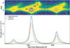 |
Fig. 1. Top: 2D spectrum of SDSS143417 around the Hα[N II] region, with gray contours tracing flux levels and blue crosses marking the positions used for Gaussian fitting. Bottom: 1D spectra extracted with different apertures: the ESO pipeline, 30 px/side, including both knots (blue), IRAF/apall, 5 px centered on the brightest knot (orange), and IRAF/apall, with asymmetric aperture sampling the secondary knot (green). Vertical dashed lines indicate the wavelength ranges where the 2D contours reveal asymmetries, serving as guides to identify additional kinematic components. |
4. Results
The results of the multicomponent line fitting and the kinematic properties obtained for the entire sample from these models are presented in Table 2. In Figures 2 and B.3, we present the multi-Gaussian fits for the galaxy sample.
Summary of the kinematic fitting results (extract).
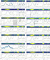 |
Fig. 2. Multi-Gaussian fitting of bright emission lines for the galaxies in our sample. Top: 2D spectra, with the y-axis in pixel units. Center: Gaussian fits of [O III]λ5007Å(left) and Hα (right). Bottom: Fit residuals. The flux axis is normalized to the peak emission of each line. Spectra are shown in light blue (labeled “Data”). The blue shadow represents the variance spectrum. The black line models the fit. The dashed lines show the different fitted components. Gray shadows are flagged regions excluded from fits. The yellow line represents the continuum. Insets that zoom in onto the faint line wings are included in the upper-right corner of each plot. |
The intrinsic velocity dispersion of the emission line (σ) is obtained from the observed velocity dispersion (σobs), after subtraction of the instrumental (σins) and thermal (σther) broadening as follows,
 (1)
(1)
where the σins corresponds to a nominal value of σins ∼ 14.3 km, s−1 for the X-shooter spectrograph in the visual arm. The thermal broadening, caused by random thermal motions of the gas, is described by
 (2)
(2)
where kB is the Boltzmann constant, mion is the ion mass, and Te is the electron temperature. In our sample, six galaxies present detections of the auroral line [O III] λ4364, with electron temperatures determined by Loaiza-Agudelo et al. (2020) ranging from 9400 to 11 900 K, with an average of ≈10 400 K. Therefore, for galaxies with no auroral line detections, we assumed Te = 10 000 K, which is consistent with the measured values and with the typical temperatures expected for H II regions in star-forming galaxies.
4.1. Emission-line kinematics
All VIS spectra show complex emission-line profiles. Single Gaussians are insufficient, as asymmetries and broad wings leave significant residuals. We used two to four Gaussian components, depending on line shape and galaxy (see Table 2). Eight galaxies required two components, four needed three, and two demanded four to reproduce their complex profiles. Following Bosch et al. (2019), the need for additional components was assessed using the Δ(AIC) > 10 criterion.
Emission lines were modeled with narrow (σ < 90 km s−1) and broad (σ > 90 km s−1) components, both resolved. This division reflects expected rotation velocities: a ∼5 × 10⁹ M⊙ galaxy rotates at ∼90 km s−1 (Simons et al. 2015). Thus, if narrow components trace disk gas, their σ should not exceed that value (see also Hogarth et al. 2020).
In Section 4.2, we further examine this assumption using the L − σ scaling relation from Terlevich & Melnick (1981). Regarding the emission measure, defined as the fraction of flux contributed by each component relative to the total line flux, we find that, in most cases, the narrow component dominates, while the broad component contributes 10–40% of the total emission.
[O III]λ5007 Å and Hα show consistent radial velocities and velocity dispersions for both components, though fitted independently. This is illustrated in Fig. B.1, which presents a comparison between σHα and σ[OIII] for our sample. While such an agreement may not necessarily be required and depends on the physical conditions and location of the gas that each component reflects, our result demonstrates robustness in determining the kinematics of ionized gas in these galaxies and suggests that recombination lines (Hα) and forbidden lines of high-ionization metal ions ([O III]) trace gas in similar regions.
Narrow-component dispersions agree with spatially resolved results from Gonçalves et al. (2010) for a subset of LBAs. Those authors found SFR-σ correlations interpreted as star formation-driven turbulence. Intense star formation injects energy into the ISM, broadening lines slightly beyond virial expectations. As we show in Sect. 4.2, our results are also consistent with an increasing velocity dispersion for galaxies with stronger star formation. High-resolution integral field unit (IFU) studies are required to disentangle rotation, turbulence, and outflows in LBAs (e.g., Bik et al. 2018; Arroyo-Polonio et al. 2024).
4.2. The luminosity of narrow and broad kinematic components
All bright lines require at least one narrow and one broad component. The narrow component traces bright star-forming regions and contributes > 80% of total flux. Their physical properties, such as dust extinction and density, show significant differences with those of the broader components, suggesting that the underlying physical mechanisms of each component also differ.
To demonstrate this difference, we analyzed the well-known L − σ correlation (Terlevich & Melnick 1981; Chávez et al. 2014), where L and σ represent the Hβ luminosity and intrinsic velocity dispersion, respectively. Giant H II regions and H II galaxies (compact low-mass starbursts) follow an L − σ relation, a robust cosmological distance indicator (Terlevich & Melnick 1981; Chávez et al. 2014; Fernández Arenas et al. 2018; Chávez et al. 2025). The underlying assumption for this correlation, which has been shown to work for low and high-redshift compact starbursts (e.g. González-Morán et al. 2021; Chávez et al. 2025), is that the narrow components of the emission lines are usually interpreted as virial motions of gas gravitationally bound to massive star clusters. However, high-resolution IFU observations of local analogs show that star formation is clumpy, with relative motions among knots that can also affect the narrow-line kinematics (Santos-Junior et al. 2025). Thus, the observed narrow components may reflect both virialized gas within clumps and relative clump-to-clump motions (see also Amorín et al. 2012b).
In Figure 3 we show the L − σ relation for 156 low and high-redshift (0 ≲ z ≲ 2.3) starbursts from Terlevich et al. (2015). We include the values for our sample, considering the individual, narrow (blue), and broad (red) components. To determine the luminosities for each component, we used the extinction-corrected Hβ flux, adopting the Calzetti (2001) extinction law. The narrow components fitted to our sample follow the L − σ relation of H II galaxies, with σHβ values up to ∼60 km, s−1. Some galaxies exhibit slightly larger σHβ for their Hβ luminosities compared to extragalactic H II regions. Ionized gas bound to massive clusters can also include clump-to-clump relative motions contributing to narrow-line kinematics. The broad components, instead, show significantly larger σHβ than expected for their Hβ luminosity if they were purely virialized, indicating the presence of an additional mechanism driving gas turbulence.
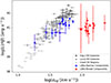 |
Fig. 3. L − σ relationship. The blue and red circles correspond to the narrow and broad components of our sample of LBA galaxies, respectively. Gray symbols are Giant HII regions and H II galaxies at 0 < z < 2.33 from Terlevich et al. (2015). |
4.3. The nature of the broad emission line components
Several mechanisms can cause line broadening in compact starbursts. These mechanisms include stellar winds from massive stars, expansion of SN remnants, outflows driven by SNe or turbulent mixing layers (TMLs), and the presence of an AGN (e.g., Izotov et al. 2007; Amorín et al. 2012b; Hogarth et al. 2020; Martin et al. 2024). Studying a sample of nearby BCDs with broad [O III] and Hα emission, Izotov et al. (2007) derive the observed Hα luminosity of the broad components (1036 − 1039 erg s−1), which are expected from the interaction between dense circumstellar envelopes around hot stars with stellar winds and/or SN remnants. The LBAs, instead, show Hα luminosities between 1040 and 1042 erg s−1 that are ∼2 dex larger than that of BCDs (Fig. 3). Such a high broad line luminosity is more typically associated with Type II SNe or an AGN.
An AGN origin is disfavored by the absence of clear nonthermal emission. The kinematics of the broad components in [O III]λ5007 Å and Hα are similar, further evidence against an AGN origin. Although an AGN cannot be ruled out, confirmation would require deep X-ray or high-resolution radio data to detect any nonthermal source. Several LBAs have already been observed in X-rays; for instance, Basu-Zych et al. (2013) reported elevated 2–10 keV luminosities relative to the SFR, consistent with enhanced high-mass X-ray binary (HMXB) populations rather than AGN activity. Previous works by Jia et al. (2011) using X-ray data and Alexandroff et al. (2012) using radio continuum observations highlight the complex challenge of confirming AGN activity and quantifying its contribution to the observed galaxy properties. In the absence of strong nonthermal signatures, the broad components are most likely powered by stellar feedback.
Turbulent mixing layers between cold disk gas and hot outflows can also broaden lines (Westmoquette et al. 2008; Binette et al. 2009). By implementing a set of TML models, Binette et al. (2009) found broad components with considerably supersonic velocities (full width at half maximum of ∼2400 km s−1). In galaxies, these high-velocity components are rarely observed in bright emission lines like [O III]λλ4959,5007 Å, Hα, and Hβ, such as in Mrk 71, a very young giant HII region (< 3Myr) belonging to the irregular dwarf galaxy NGC 2366 (Komarova et al. 2021), or in the giant H II region NGC 5471 (Castaneda et al. 1990). However, TML models generally assume a high-ionization parameter log(U), leading the ionization throughout the turbulent layer, thus making the gas dominated by highly excited species and therefore struggling to explain such components in low-ionization forbidden lines, such as [NII] or [SII] (Binette et al. 2009). For example, Bosch et al. (2019) and Hogarth et al. (2020) discussed TMLs as one of the mechanisms to explain the complex kinematics of Green Pea galaxies showing broad components in [NII] and [SII], concluding that a TML model would require a low log(U) (Binette et al. 2009). However, using the [O II]/[O III] ratio of GP 1429, Hogarth et al. (2020) found a relatively high log(U) for the broad component, disfavoring the TML interpretation.
In the LBAs, we do not find broad components reaching such high velocities of > 1000km s−1. LBAs show no > 1000km s−1 broad components and display relatively high log(U) (−2.9 to −2.3 Loaiza-Agudelo et al. 2020). This, along with the relatively modest velocities found by our fittings of both low- and high-ionization lines, suggests that the broadening of the faint line wings cannot be entirely explained by TMLs. TML contributions cannot be excluded, but detailed modeling and high-dispersion IFU mapping are needed to test them.
Finally, shocks produced by young SN remnants can significantly contribute to the turbulence of ionized gas. According to Ho et al. (2014), the contributions of shock processes can be identified in diagnostic diagrams by the presence of broad components with higher [NII], [SII], and [O II] to Hα ratios, as well as elevated electron density values. Therefore, a scenario with a strong contribution from stellar feedback and shocks from SN remnants is a likely mechanism for providing energy to the turbulent ionized gas in these star-forming galaxies, resulting in high velocity dispersions in the broad components. Given the low broad-to-narrow luminosity ratios and lack of AGN signatures, stellar winds and SN feedback likely power the broad emission.
4.4. Emission-line diagnostics
We examined classic emission-line diagnostic diagrams using our multi-Gaussian fits. Our goal was to assess excitation properties and the dominant ionization mechanism of each component. We show in Fig. 4 the diagnostic diagrams based on the [O III]λ5007/Hβ versus [N II]λ6584/Hα relation (Baldwin et al. 1981) and [S II]λλ6716,6731/Hα (Veilleux & Osterbrock 1987). In Fig. 4 we show the ratios based on integrated line flux for each galaxy with gray squares. Blue and red circles show instead the ratios for the narrow (σ ≲ 90 km s−1) and broad (σ ≳ 90 km s−1) components. For comparison, we show SDSS galaxies and the different theoretical and empirical demarcation lines, which allow us to constrain the ionization source for each component. Most galaxies are consistent with stellar photoionization; only SDSS021348 shows elevated N2 and S2 ratios typical of low-ionization nuclear emission-line regions.
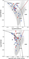 |
Fig. 4. Classic diagnostic diagrams based on emission line ratios (Baldwin et al. 1981; Veilleux & Osterbrock 1987): [O III]λ5007/Hβ vs. [NII]λ6584/Hα (top) and [O III]λ5007/ Hβ vs. [S II]λλ6716.6731/Hα (bottom). Symbols show the emission-line–integrated fluxes (gray squares) and narrow (blue circles) and broad (red circles) Gaussian components for each galaxy. The gray dots correspond to the SDSS-DR7 MPA-JHU galaxy sample from Pérez-Montero et al. (2021). Regions of different excitation mechanisms are labeled and established by the theoretical and empirical demarcation lines of Kewley et al.; Kewley et al. (2001; 2006, dashed black), Kauffmann et al. (2003, dashed gray), and Schawinski et al. (2007), solid brown). |
There is a small fraction of galaxies showing kinematic components within the so-called “composite” region, thus allowing a contribution of shocks or some nuclear activity. Three galaxies, SDSS001009, SDSS005527, and SDSS015028 have their kinematic components consistent with high ionization AGN Seyfert II excitation.
Overall, no systematic trend appears among the three diagnostic ratios in Fig. 4. In particular, the broad components are not associated with a different excitation mechanism compared to the narrow components, and both are consistent with the conclusions one can obtain from the integrated line ratios.
4.5. Electron density
Electron density (ne) is key to characterizing physical conditions in star-forming regions, together with electron temperature. We determined ne using the Sulfur doublet [S II]λλ6716/6731 Å because it is present in the entire sample and because the [O II]λλ3726/3729 Å doublet is observed in the UBV arm of X-shooter and therefore its spectral resolution is a factor of ∼1.65 lower. We computed ne using Specsy (Fernández et al. 2023). The electron temperatures for 6 galaxies (SDSS004054, SDSS005527, SDSS015028, SDSS020356, SDSS032845, SDSS235347) were taken from Loaiza-Agudelo et al. (2020). For the remaining eight galaxies without Te measurements, we assumed Te = 10 000 K.
Table A.1 includes the density values obtained for the integrated flux ratios and for those of the different kinematic components following the above methodology. Electron densities range from 120 cm−3 to 1416 cm−3 with (narrow) and 366 cm−3 (broad). For some galaxies (SDSS005527, SDSS020356, SDSS214500, and SDSS231812), the broad components show higher density than the narrow components. Two galaxies (SDSS015028 and SDSS0035733) show all the narrow, broad, and integrated components with very similar densities. Finally, three galaxies (SDSS021348, SDSS032845, and SDSS232539) show denser narrow components compared to the broad components.
While we acknowledge that the large uncertainties inherent to the electron density estimates may affect the analysis, our results suggest that different kinematic components have different density conditions according to their [S II] ratios. These variations likely reflect the diversity in physical and dynamical conditions among LBAs. For example, effects such as the compactness, age, and ionization conditions of the bright star-forming regions may result in different gas pressure conditions for the narrow components tracing H II gas. Similarly, the presence of denser broad components tracing outflows can be the result of shocked gas due to SN feedback and the interacting/merger nature of some of the galaxies, which appears consistent with our analysis based on classic emission-line diagnostics (e.g., Ho et al. 2014; Rodríguez del Pino et al. 2019). For example, the electron density of the outflow components is consistent with those derived from stacked spectra of galaxies at z ∼ 0.6 − 2.7, which are about 400 cm−3 (Förster Schreiber et al. 2019). Overall, the ne values of both components agree with those in other UV-bright starbursts and local high-z analogs (e.g., Arribas et al. 2014; Hogarth et al. 2020; Álvarez-Márquez et al. 2021; Amorín et al. 2024; Martin et al. 2024).
We also compared our ne estimates with those reported by Loaiza-Agudelo et al. (2020) for the same LBA sample. Their analysis, based on single-component fits to the [S II] doublet, yields average densities around 160 cm−3, whereas our global median values are somewhat higher, around 300 cm−3. This difference is likely due to our multicomponent Gaussian fitting approach, which allows us to isolate and quantify denser kinematic components that contribute to the total emission. These results suggest that integrated single-component measurements underestimate the density of the outflowing ionized gas when multiple components are present.
4.6. Outflow properties
From the L − σ relation (Sect. 4.2), the broad components trace gas that has been accelerated beyond typical H II region dynamics. These highly turbulent components are identified as ionized outflows, likely denser and more compact than those traced by UV absorption lines. Its origin is probably a combination of gas driven by the combined action of strong stellar winds from massive stars, SN explosions, and shocks originating from galaxy interactions.
We derived outflow properties from the broad components, following equations in Concas et al. (2022) and Llerena et al. (2023). Table 3 shows a summary of our results. We first focus on the outflow gas mass, which can be estimated as
 (3)
(3)
Outflow properties.
Where  corresponds to the broadest component of the emission line of Hα, which was extinction-corrected using Calzetti (2001). Following Llerena et al. (2023), we use Hα instead of [O III] since [O III]-based masses depend on poorly constrained metallicity effects. In Eq. 3, ne is the density of the broad component. In cases where the density of the broad component cannot be derived, we use the global density measured from the integrated line ratios (Table A.1). Assuming a multi-cone or spherical geometry, the outflow mass rate (Ṁout) is defined Lutz et al. (2020) as
 (4)
(4)
where C depends on the assumed outflow history, Rout is the outflow radius, Mout is the outflow mass and Vout is the outflow velocity.
Following Llerena et al. (2023), we adopted C = 1 which corresponds to assuming that the wind mass rate is constant. To be consistent with previous works, we defined the outflow velocity as Vout = ∣ΔVr − 2 × σBroad∣ (Genzel et al. 2011), where we used the intrinsic velocity dispersion of Hα. As shown in Fig. B.2, using instead [O III]λ5007 Å has a negligible impact on the final results. For the outflow radius, we assumed Rout = Re (Förster Schreiber et al. 2019) which is justified by the typical sizes of ionized gas outflows detected with high-resolution adaptive-optics–assisted SINFONI observations for a sample of high-z galaxies (see Newman et al. (2012) and Förster Schreiber et al. (2014)). Applying Eq. (4) yields Ṁout = 0.20−2.72 M⊙ yr−1 (⟨Ṁout⟩ = 1.43 M⊙ yr−1).
Finally, we obtained the mass loading factor (η) as
 (5)
(5)
where Ṁout is obtained with Eq. (4) and SFRnarrow is determined using the luminosity of Hα, taking into account only the narrow component and applying the extinction correction described by Overzier et al. (2009). We note that our SFR values are systematically lower than those reported by Overzier et al. (2009) for the same objects. This is expected, since they used SDSS spectra and applied an aperture correction factor of ∼1.7 to recover the total galaxy flux, while our estimates are based on VLT/X-shooter data and refer only to the narrow component. In addition, the broad component contributes a smaller but non-negligible fraction to the total Hα flux, partially accounting for this difference.
The mass-loading factor is a crucial parameter for understanding how outflows affect the properties of galaxies. This factor quantifies the efficiency with which outflows remove gas from the galaxy relative to the SFR. The mass-loading factors span η = 0.03 − 0.81 (mean ⟨η⟩ = 0.31).
The values of outflow properties for our sample are summarized in Table 3. In Sect. 5, we discuss these results and how they contribute to our understanding of starburst-driven feedback.
5. Discussion
5.1. Comparison with previous works
Our sample of LBAs shows complex emission lines with both narrow and broad components. The velocity dispersion of the narrow components agrees with that reported by Gonçalves et al. (2010) from the central (∼1″) Paschen α emission of LBAs, who found relatively high mean values (∼70 km s−1) indicative of turbulent gas kinematics. However, Gonçalves et al. (2010) did not detect clear high-velocity components, possibly due to the shallower depth of their NIR data.
For the nine galaxies overlapping with Gonçalves et al. (2010), our kinematics agree closely. This suggests that highly turbulent ionized gas kinematics is common in LBAs, with values exceeding those of Giant HII regions in spiral galaxies (e.g. Firpo et al. 2010) and similar to spectroscopically selected starburst galaxies in the local universe (e.g. Östlin et al. 2001; Green et al. 2010; Amorín et al. 2012b; Chávez et al. 2014).
The ionized gas emission of the narrow components follows the L − σ relation shown in Fig. 3 (Terlevich & Melnick 1981, see Sect. 4.2), implying gas gravitationally bound to massive star clusters. Additional sources of energy contributing to the observed turbulence may include stellar feedback and local enhancements, such as shocks driven by interactions or mergers (e.g. Baron et al. 2024; Martin et al. 2024). This could explain some LBAs located in the outer envelope of that relation (Fig. 3), originally defined for young extragalactic H II regions.
Morphologically, the sample is diverse, including compact galaxies with a dominant central source and spatially extended systems showing tidal features (Overzier et al. 2009). In several extended LBAs, the two-dimensional X-shooter spectra are spatially resolved, revealing complex velocity fields. These characteristics resemble those of other local analogs to high-redshift galaxies, such as Haro 11 (Östlin et al. 2009; Bik et al. 2018) or the BCDs studied by Bik et al. (2022). Overall, the complex ionized-gas kinematics of LBAs likely reflects a disturbed gas morphology, with strong gravitational instabilities affecting both stars and gas, probably driven by mergers or accretion events.
Their kinematics thus appear dominated by turbulence rather than ordered rotation, similar to low-mass starbursts at higher redshift (e.g. Wisnioski et al. 2015; Simons et al. 2015). Recently, de Graaff et al. (2024) analyzed the gas kinematics of star-forming galaxies at 5.5 < z < 7.4 using JWST/NIRSpec R2700 spectra, finding comparable stellar masses, sizes, and velocity structures to LBAs, characterized by broadened lines, modest gradients, and mixed rotational–dispersion support with σ ∼ 30 − 70 km s−1. These parallels reinforce the role of LBAs as nearby laboratories for studying the physical processes that shape galaxies in the early Universe.
5.2. Trends for outflow rates and mass loading with stellar mass and compact star formation
The turbulent gas kinematics of LBAs include high-velocity components detected in the wings of [O III] and Balmer lines, which we interpret as signatures of ionized outflows. Examining the relations between the derived outflow properties and the global characteristics of their host galaxies provides valuable clues about feedback processes.
Figure 5 (left) shows the relation between η and stellar mass for star-forming galaxies at low (Marasco et al. 2023; McQuinn et al. 2019) and high redshift (Concas et al. 2022; Llerena et al. 2023; Weldon et al. 2024; Carniani et al. 2024; Saldana-Lopez et al. 2025; Xu et al. 2025b) from deep spectroscopic surveys. Although the stellar-mass range of the LBA sample is narrow, they are indistinguishable from LBGs at z ∼ 2–3 and follow the same trend exhibited by low-mass LBGs at z ≳ 3–9.
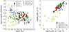 |
Fig. 5. Outflow mass loading factor as a function of the stellar mass of galaxies (left) and stellar mass outflow rate as a function of SFR surface density (right). Our LBAs are shown as red squares. Green and black circles are LBGs at z ∼ 1.4 − 3.8 from Weldon et al. (2024) and Llerena et al. (2023), respectively, while purple stars are mean-weighted averages from stacks of star-forming galaxies at z ∼ 2.1 from Concas et al. (2022). Gray and blue crosses are low-mass star-forming galaxies at z ∼ 3 − 9 observed with JWST/NIRSpec R = 2700 spectroscopy from Carniani et al. (2024) and Saldana-Lopez et al. (2025), respectively. The green crosses are the results from Xu et al. (2025b) for galaxies at z ∼ 3 − 9. Yellow stars are local dwarf galaxies from Marasco et al. (2023). Light blue squares indicate local dwarf galaxies from McQuinn et al. (2019). Dashed red lines are rescaled relations from Ilustris-TNG simulations of Nelson et al. (2019), and dashed black lines are from FIRE-2 simulations of Pandya et al. (2021). |
Overall, LBA results agree with those for high-z galaxies (z ∼ 3) by Llerena et al. (2023) based on high-resolution long-slit spectra, including LBGs from Llerena et al. (2022) and strong Lyα emitters (Amorín et al. 2017). In the stellar-mass range M★ ∼ 109–1010 M⊙, our findings are also consistent with Weldon et al. (2024), who used composite MOSDEF spectra of LBGs at z ∼ 1.4–3.8 (medium-resolution, unresolved). In contrast, our LBAs show larger loading factors at fixed stellar mass than the stacked IFU spectra of main-sequence galaxies at z ∼ 2 by Concas et al. (2022). While the η–M★ trend is similar, the offset likely arises from methodological differences such as lower-resolution IFU data, spectral stacking, or distinct separation of virial and non-virial components in line profiles. At higher redshifts, we find good agreement with the trends reported by Carniani et al. (2024) and Saldana-Lopez et al. (2025) using JWST/NIRSpec R2700 spectra, showing a continuous sequence from high- to low-mass, strongly star-forming galaxies with increasing η. Similarly, Xu et al. (2025b) and Cooper et al. (2025) derived η values between 0.1 and 10 for low-mass galaxies at z > 3, displaying comparable trends and large scatter with stellar mass.
Compared with local samples, our results follow the relation found at lower masses (M★ ∼ 107–109 M⊙) by McQuinn et al. (2019), confirming that low-mass star-forming galaxies strongly influence the outflow mass-loading factor. However, our sample shows an offset relative to nearby dwarf galaxies observed with spatially resolved MUSE data by Marasco et al. (2023), who report a different trend and generally lower η. As for the comparison with Concas et al. (2022), such differences likely stem from the diverse methodologies used to derive outflow properties (see also Saldana-Lopez et al. 2025).
In Fig. 5 we also include predictions from the Illustris-TNG (Nelson et al. 2019) and FIRE-2 (Pandya et al. 2021) simulations, rescaled for comparison with the data. Illustris-TNG predicts a characteristic decrease in η in the range 108.5 < M★/M⊙ < 1010.5, followed by a sharp rise for more massive systems, whereas FIRE-2 shows a monotonic decline from low to high stellar mass, extending down to M★ ∼ 107 M⊙. The observed LBA and LBG trends are broadly consistent with the predicted higher η in low-mass systems due to their shallower potential wells (e.g., Nelson et al. 2019; Pandya et al. 2021), though the scatter remains substantial (0.5–1 dex) in the lowest-mass bins.
The right panel of Fig. 5 compares outflow rates Ṁout with SFR surface density ΣSFR for the same samples. We find a clear relation between more compact galaxies (higher ΣSFR) and larger Ṁout, in excellent agreement with high-z LBG studies (e.g. Llerena et al. 2023; Weldon et al. 2024; Saldana-Lopez et al. 2025). Even the local MUSE sample of Marasco et al. (2023) follows a similar, though lower, normalization.
Following the conclusions of Llerena et al. (2023), a higher Ṁout in denser starbursts may explain the scatter in η at fixed M★. Using high-resolution spectra of local star-forming galaxies (including some LBAs), Xu et al. (2025a) found that outflow velocities from optical lines reach 60–70% of those from UV absorption, yielding outflow rates ∼0.2–0.5 dex lower (see also Heckman et al. 2011; Borthakur et al. 2014). These results suggest that the discrepancies arise from the different density regimes probed by emission versus absorption diagnostics.
Future studies combining emission- and absorption-line tracers in this and other local analog samples (e.g. green pea galaxies; Amorín et al. 2024) will help clarify how density effects contribute to the observed scatter in these scaling relations and their implications for high-redshift studies.
6. Conclusions
We analyzed the ionized-gas kinematics and outflow properties of 14 compact, UV-luminous galaxies at z < 0.2 – the so-called LBAs–using deep, high-resolution (R ∼ 8900) VLT/X-shooter visible spectra. Our analysis involved detailed modeling of Hβ, [O III]λλ4959,5007 Å, Hα, [NII]λλ6548,6584 Å, and [S II]λλ6716,6731 Å line profiles, adopting a tailored multi-Gaussian fitting approach with the LiMe software (Fernández et al. 2024). Our main results are summarized as follows:
-
Lyman-break analogs exhibit complex emission-line profiles that deviate from a single Gaussian model, requiring two to four components for an accurate representation. They include one or more narrow components with intrinsic dispersions (σint) of ∼20–70 km s−1, Hβ luminosities of 1040–1041 erg s−1, and at least one broad component with σint of ∼90–250 km s−1. For 9 of the 14 galaxies, the broad components are blueshifted (ΔVr ∼ 4–86 km s−1) and contribute ∼13–60% of the total flux in both recombination and collisionally excited lines.
-
From the L(Hβ)–σ relation for giant extragalactic H II regions and H II galaxies, the narrow components trace virialized gas near young star clusters, while the broad components correspond to high-velocity outflows likely driven by stellar winds and SNe. Classical diagnostics indicate that stellar photoionization is the main ionizing source, although shocks may contribute to the broad emission in some objects.
-
Electron densities (ne) from the [SII] doublet span ∼100–1400 cm−3, consistent with other UV-bright starbursts. Densities for narrow and broad components are often comparable, although in some galaxies the higher ne of the broad gas suggests pressurized or shock-heated regions produced by stellar feedback or interactions.
-
Using broad-component measurements and a simple outflow model, we derived mass-loss rates of 0.20–2.72 M⊙ yr−1 (mean 1.4 M⊙ yr−1) and mass-loading factors (η) of 0.03–0.81 (mean 0.31), consistent with the mean η of 0.54 found for LBGs at z ∼ 3 (Llerena et al. 2023). Combining this with results for lower-mass starbursts at low and high redshifts, we find a mild increase in η toward lower stellar masses and larger Ṁout at higher SFR surface densities. Low-mass galaxies undergoing intense starbursts thus develop strong outflows with similar properties across redshift, modulated by the compactness of star formation. When derived with comparable methods and assumptions, their outflow properties follow the predicted η–M★ trends from simulations.
In summary, the multi-Gaussian modeling reveals the strong complexity of the ionized-gas kinematics in LBAs. Our findings are consistent with those for high-redshift LBGs and highlight the role of dense, metal-poor starbursts in shaping outflows and stellar feedback in low-mass galaxies. This highlights LBAs as key laboratories for investigating star formation and feedback under ISM conditions akin to those at high redshifts. Future high-dispersion, spatially resolved (IFU) spectroscopy across multiple wavelengths will be essential to linking global gas kinematics, multiphase outflow properties, and star formation in low-mass starbursts.
Data availability
The full version of Table 2, which includes additional emission lines, is available at the CDS via https://cdsarc.cds.unistra.fr/viz-bin/cat/J/A+A/707/A13
Acknowledgments
We are grateful to Verónica Firpo for her valuable guidance on emission-line fitting at the early stages of this work. We thank Alberto Saldana-Lopez for providing tables with comparison data. AL and RA acknowledge support from ULS/DIDULS grant PTE2153851. AL and RA acknowledge support from ANID Fondecyt 1202007. RA acknowledges support of grant PID2023-147386NB-I00 funded by MICIU/AEI/10.13039/501100011033 and by ERDF/EU, from grant PID2022-136598NBC32 “Estallidos8”, and the Severo Ochoa grant CEX2021-001131-S to the IAA-CSIC. MLl acknowledges support from the INAF Large Grant 2022 “Extragalactic Surveys with JWST” (PI L. Pentericci), the PRIN 2022 MUR project 2022CB3PJ3 – First Light And Galaxy aSsembly (FLAGS) funded by the European Union – Next Generation EU, and the INAF Mini-grant “Galaxies in the epoch of Reionization and their analogs at lower redshift” (PI M. Llerena).
References
- Alexandroff, R., Overzier, R. A., Paragi, Z., et al. 2012, MNRAS, 423, 1325 [Google Scholar]
- Alexandroff, R. M., Heckman, T. M., Borthakur, S., Overzier, R., & Leitherer, C. 2015, ApJ, 810, 104 [Google Scholar]
- Álvarez-Márquez, J., Marques-Chaves, R., Colina, L., & Pérez-Fournon, I. 2021, A&A, 647, A133 [NASA ADS] [CrossRef] [EDP Sciences] [Google Scholar]
- Amorín, R. O., Pérez-Montero, E., & Vílchez, J. M. 2010, ApJ, 715, L128 [CrossRef] [Google Scholar]
- Amorín, R., Pérez-Montero, E., Vílchez, J. M., & Papaderos, P. 2012a, ApJ, 749, 185 [CrossRef] [Google Scholar]
- Amorín, R., Vílchez, J. M., Hägele, G. F., et al. 2012b, ApJ, 754, L22 [CrossRef] [Google Scholar]
- Amorín, R., Fontana, A., Pérez-Montero, E., et al. 2017, Nat. Astron., 1, 0052 [Google Scholar]
- Amorín, R. O., Rodríguez-Henríquez, M., Fernández, V., et al. 2024, A&A, 682, L25 [NASA ADS] [CrossRef] [EDP Sciences] [Google Scholar]
- Araujo-Carvalho, A. E., Gonçalves, T. S., Krajnović, D., Menéndez-Delmestre, K., & de Isídio, N. 2025, ApJ, 991, 3 [Google Scholar]
- Arrabal Haro, P., Dickinson, M., Finkelstein, S. L., et al. 2023, ApJ, 951, L22 [NASA ADS] [CrossRef] [Google Scholar]
- Arribas, S., Colina, L., Bellocchi, E., Maiolino, R., & Villar-Martín, M. 2014, A&A, 568, A14 [NASA ADS] [CrossRef] [EDP Sciences] [Google Scholar]
- Arroyo-Polonio, A., Kehrig, C., Iglesias-Páramo, J., et al. 2024, A&A, 687, A77 [NASA ADS] [CrossRef] [EDP Sciences] [Google Scholar]
- Baldwin, J. A., Phillips, M. M., & Terlevich, R. 1981, PASP, 93, 5 [Google Scholar]
- Baron, D., Netzer, H., Lutz, D., Davies, R. I., & Prochaska, J. X. 2024, ApJ, 968, 23 [NASA ADS] [CrossRef] [Google Scholar]
- Basu-Zych, A. R., Gonçalves, T. S., Overzier, R., et al. 2009a, ApJ, 699, L118 [Google Scholar]
- Basu-Zych, A. R., Schiminovich, D., Heinis, S., et al. 2009b, ApJ, 699, 1307 [Google Scholar]
- Basu-Zych, A. R., Lehmer, B. D., Hornschemeier, A. E., et al. 2013, ApJ, 762, 45 [NASA ADS] [CrossRef] [Google Scholar]
- Bik, A., Östlin, G., Menacho, V., et al. 2018, A&A, 619, A131 [NASA ADS] [CrossRef] [EDP Sciences] [Google Scholar]
- Bik, A., Östlin, G., Hayes, M., Melinder, J., & Menacho, V. 2022, A&A, 666, A161 [NASA ADS] [CrossRef] [EDP Sciences] [Google Scholar]
- Binette, L., Flores-Fajardo, N., Raga, A. C., Drissen, L., & Morisset, C. 2009, ApJ, 695, 552 [NASA ADS] [CrossRef] [Google Scholar]
- Borthakur, S., Heckman, T. M., Leitherer, C., & Overzier, R. A. 2014, Science, 346, 216 [Google Scholar]
- Bosch, G., Hägele, G. F., Amorín, R., et al. 2019, MNRAS, 489, 1787 [NASA ADS] [CrossRef] [Google Scholar]
- Bouwens, R. J., Oesch, P. A., Stefanon, M., et al. 2021, AJ, 162, 47 [NASA ADS] [CrossRef] [Google Scholar]
- Brown, J. S., Croxall, K. V., & Pogge, R. W. 2014, ApJ, 792, 140 [Google Scholar]
- Bunker, A. J., Cameron, A. J., Curtis-Lake, E., et al. 2024, A&A, 690, A288 [NASA ADS] [CrossRef] [EDP Sciences] [Google Scholar]
- Calzetti, D. 2001, PASP, 113, 1449 [Google Scholar]
- Carniani, S., Venturi, G., Parlanti, E., et al. 2024, A&A, 685, A99 [NASA ADS] [CrossRef] [EDP Sciences] [Google Scholar]
- Castaneda, H. O., Vilchez, J. M., & Copetti, M. V. F. 1990, ApJ, 365, 164 [NASA ADS] [CrossRef] [Google Scholar]
- Chávez, R., Terlevich, R., Terlevich, E., et al. 2014, MNRAS, 442, 3565 [CrossRef] [Google Scholar]
- Chávez, R., Terlevich, R., Terlevich, E., et al. 2025, MNRAS, 538, 1264 [Google Scholar]
- Concas, A., Maiolino, R., Curti, M., et al. 2022, MNRAS, 513, 2535 [NASA ADS] [CrossRef] [Google Scholar]
- Contursi, A., Baker, A. J., Berta, S., et al. 2017, A&A, 606, A86 [NASA ADS] [CrossRef] [EDP Sciences] [Google Scholar]
- Cooper, R. A., Caputi, K. I., Iani, E., et al. 2025, ApJ, 994, 102 [Google Scholar]
- Cullen, F., McLure, R. J., Dunlop, J. S., et al. 2019, MNRAS, 487, 2038 [Google Scholar]
- de Graaff, A., Rix, H.-W., Carniani, S., et al. 2024, A&A, 684, A87 [NASA ADS] [CrossRef] [EDP Sciences] [Google Scholar]
- Fernández Arenas, D., Terlevich, E., Terlevich, R., et al. 2018, MNRAS, 474, 1250 [Google Scholar]
- Fernández, V., Amorín, R., Sanchez-Janssen, R., del Valle-Espinosa, M. G., & Papaderos, P. 2023, MNRAS, 520, 3576 [CrossRef] [Google Scholar]
- Fernández, V., Amorín, R., Firpo, V., & Morisset, C. 2024, A&A, 688, A69 [NASA ADS] [CrossRef] [EDP Sciences] [Google Scholar]
- Finkelstein, S. L., Leung, G. C. K., Bagley, M. B., et al. 2024, ApJ, 969, L2 [NASA ADS] [CrossRef] [Google Scholar]
- Firpo, V., Bosch, G., Hägele, G. F., & Morrell, N. 2010, MNRAS, 406, 1094 [Google Scholar]
- Firpo, V., Bosch, G., Hägele, G. F., Díaz, n. I., & Morrell, N. 2011, MNRAS, 414, 3288 [NASA ADS] [CrossRef] [Google Scholar]
- Fischer, C. F., & Tachiev, G. 2004, At. Data Nucl. Data Tables, 87, 1 [NASA ADS] [CrossRef] [Google Scholar]
- Förster Schreiber, N. M., Genzel, R., Newman, S. F., et al. 2014, ApJ, 787, 38 [Google Scholar]
- Förster Schreiber, N. M., Übler, H., Davies, R. L., et al. 2019, ApJ, 875, 21 [Google Scholar]
- Genzel, R., Newman, S., Jones, T., et al. 2011, ApJ, 733, 101 [Google Scholar]
- Giavalisco, M. 2002, ARA&A, 40, 579 [Google Scholar]
- Gonçalves, T. S., Basu-Zych, A., Overzier, R., et al. 2010, ApJ, 724, 1373 [CrossRef] [Google Scholar]
- Gonçalves, T. S., Basu-Zych, A., Overzier, R. A., Pérez, L., & Martin, D. C. 2014, MNRAS, 442, 1429 [Google Scholar]
- González-Morán, A. L., Chávez, R., Terlevich, E., et al. 2021, MNRAS, 505, 1441 [CrossRef] [Google Scholar]
- Green, A. W., Glazebrook, K., McGregor, P. J., et al. 2010, Nature, 467, 684 [NASA ADS] [CrossRef] [Google Scholar]
- Heckman, T. M., & Borthakur, S. 2016, ApJ, 822, 9 [CrossRef] [Google Scholar]
- Heckman, T. M., Hoopes, C. G., Seibert, M., et al. 2005, ApJ, 619, L35 [NASA ADS] [CrossRef] [Google Scholar]
- Heckman, T. M., Borthakur, S., Overzier, R., et al. 2011, ApJ, 730, 5 [Google Scholar]
- Heckman, T. M., Alexandroff, R. M., Borthakur, S., Overzier, R., & Leitherer, C. 2015, ApJ, 809, 147 [Google Scholar]
- Ho, I. T., Kewley, L. J., Dopita, M. A., et al. 2014, MNRAS, 444, 3894 [Google Scholar]
- Hogarth, L., Amorín, R., Vílchez, J. M., et al. 2020, MNRAS, 494, 3541 [NASA ADS] [CrossRef] [Google Scholar]
- Hoopes, C. G., Heckman, T. M., Salim, S., et al. 2007, ApJS, 173, 441 [NASA ADS] [CrossRef] [Google Scholar]
- Izotov, Y. I., Thuan, T. X., & Guseva, N. G. 2007, ApJ, 671, 1297 [NASA ADS] [CrossRef] [Google Scholar]
- Jia, J., Ptak, A., Heckman, T. M., et al. 2011, ApJ, 731, 55 [NASA ADS] [CrossRef] [Google Scholar]
- Kauffmann, G., Heckman, T. M., Tremonti, C., et al. 2003, MNRAS, 346, 1055 [Google Scholar]
- Kewley, L. J., Dopita, M. A., Sutherland, R. S., Heisler, C. A., & Trevena, J. 2001, ApJ, 556, 121 [Google Scholar]
- Kewley, L. J., Groves, B., Kauffmann, G., & Heckman, T. 2006, MNRAS, 372, 961 [Google Scholar]
- Komarova, L., Oey, M. S., Krumholz, M. R., et al. 2021, ApJ, 920, L46 [NASA ADS] [CrossRef] [Google Scholar]
- Le Fèvre, O., Tasca, L. A. M., Cassata, P., et al. 2015, A&A, 576, A79 [Google Scholar]
- Llerena, M., Amorín, R., Cullen, F., et al. 2022, A&A, 659, A16 [NASA ADS] [CrossRef] [EDP Sciences] [Google Scholar]
- Llerena, M., Amorín, R., Pentericci, L., et al. 2023, A&A, 676, A53 [NASA ADS] [CrossRef] [EDP Sciences] [Google Scholar]
- Loaiza-Agudelo, M., Overzier, R. A., & Heckman, T. M. 2020, ApJ, 891, 19 [CrossRef] [Google Scholar]
- Lutz, D., Sturm, E., Janssen, A., et al. 2020, A&A, 633, A134 [NASA ADS] [CrossRef] [EDP Sciences] [Google Scholar]
- Maiolino, R., Nagao, T., Grazian, A., et al. 2008, A&A, 488, 463 [NASA ADS] [CrossRef] [EDP Sciences] [Google Scholar]
- Marasco, A., Belfiore, F., Cresci, G., et al. 2023, A&A, 670, A92 [NASA ADS] [CrossRef] [EDP Sciences] [Google Scholar]
- Martin, C. L., Peng, Z., & Li, Y. 2024, ApJ, 966, 190 [Google Scholar]
- Matthee, J., Sobral, D., Hayes, M., et al. 2021, MNRAS, 505, 1382 [NASA ADS] [CrossRef] [Google Scholar]
- McQuinn, K. B. W., van Zee, L., & Skillman, E. D. 2019, ApJ, 886, 74 [NASA ADS] [CrossRef] [Google Scholar]
- Melnick, J., Tenorio-Tagle, G., & Terlevich, R. 1999, MNRAS, 302, 677 [Google Scholar]
- Modigliani, A., Goldoni, P., Royer, F., et al. 2010, SPIE Conf. Ser., 7737, 773728 [Google Scholar]
- Muratov, A. L., Kereš, D., Faucher-Giguère, C.-A., et al. 2015, MNRAS, 454, 2691 [NASA ADS] [CrossRef] [Google Scholar]
- Nelson, D., Pillepich, A., Springel, V., et al. 2019, MNRAS, 490, 3234 [Google Scholar]
- Newman, S. F., Genzel, R., Förster-Schreiber, N. M., et al. 2012, ApJ, 761, 43 [Google Scholar]
- Newville, M., Stensitzki, T., Allen, D., & Ingargiola, A. 2014, https://doi.org/10.5281/zenodo.11813 [Google Scholar]
- Östlin, G., Amram, P., Bergvall, N., et al. 2001, A&A, 374, 800 [NASA ADS] [CrossRef] [EDP Sciences] [Google Scholar]
- Östlin, G., Hayes, M., Kunth, D., et al. 2009, AJ, 138, 923 [NASA ADS] [CrossRef] [Google Scholar]
- Overzier, R. A., Heckman, T. M., Kauffmann, G., et al. 2008, ApJ, 677, 37 [Google Scholar]
- Overzier, R. A., Heckman, T. M., Tremonti, C., et al. 2009, ApJ, 706, 203 [NASA ADS] [CrossRef] [Google Scholar]
- Pandya, V., Fielding, D. B., Anglé s-Alcázar, D., et al. 2021, MNRAS, 508, 2979 [NASA ADS] [CrossRef] [Google Scholar]
- Peng, Y.-J., Lilly, S. J., Kovač, K., et al. 2010, ApJ, 721, 193 [Google Scholar]
- Pentericci, L., McLure, R. J., Garilli, B., et al. 2018, A&A, 616, A174 [NASA ADS] [CrossRef] [EDP Sciences] [Google Scholar]
- Pérez-Montero, E., Amorín, R., Sánchez Almeida, J., et al. 2021, MNRAS, 504, 1237 [CrossRef] [Google Scholar]
- Robertson, B. E., Ellis, R. S., Furlanetto, S. R., & Dunlop, J. S. 2015, ApJ, 802, L19 [Google Scholar]
- Rodríguez del Pino, B., Arribas, S., Piqueras López, J., Villar-Martín, M., & Colina, L. 2019, MNRAS, 486, 344 [CrossRef] [Google Scholar]
- Rodríguez Del Pino, B., Perna, M., Arribas, S., et al. 2024, A&A, 684, A187 [NASA ADS] [CrossRef] [EDP Sciences] [Google Scholar]
- Saldana-Lopez, A., Chisholm, J., Gazagnes, S., et al. 2025, MNRAS, 544, 132 [Google Scholar]
- Santana-Silva, L., Gonçalves, T. S., Basu-Zych, A., et al. 2020, MNRAS, 498, 5183 [Google Scholar]
- Santos-Junior, J. M., Gonçalves, T. S., Santana-Silva, L., et al. 2025, ApJ, 987, 90 [Google Scholar]
- Sawala, T., Frenk, C. S., Fattahi, A., et al. 2016, MNRAS, 456, 85 [Google Scholar]
- Schawinski, K., Thomas, D., Sarzi, M., et al. 2007, MNRAS, 382, 1415 [Google Scholar]
- Shapley, A. E., Steidel, C. C., Adelberger, K. L., et al. 2001, ApJ, 562, 95 [NASA ADS] [CrossRef] [Google Scholar]
- Shapley, A. E., Steidel, C. C., Pettini, M., & Adelberger, K. L. 2003, ApJ, 588, 65 [Google Scholar]
- Simons, R. C., Kassin, S. A., Weiner, B. J., et al. 2015, MNRAS, 452, 986 [Google Scholar]
- Steidel, C. C., Giavalisco, M., Pettini, M., Dickinson, M., & Adelberger, K. L. 1996, ApJ, 462, L17 [Google Scholar]
- Storey, P., & Zeippen, C. 2000, MNRAS, 312, 813 [NASA ADS] [CrossRef] [Google Scholar]
- Terlevich, R., & Melnick, J. 1981, MNRAS, 195, 839 [NASA ADS] [CrossRef] [Google Scholar]
- Terlevich, R., Terlevich, E., Melnick, J., et al. 2015, MNRAS, 451, 3001 [NASA ADS] [CrossRef] [Google Scholar]
- Tumlinson, J., Peeples, M. S., & Werk, J. K. 2017, ARA&A, 55, 389 [Google Scholar]
- Veilleux, S., & Osterbrock, D. E. 1987, ApJS, 63, 295 [Google Scholar]
- Virtanen, P., Gommers, R., Oliphant, T. E., et al. 2020, Nat. Methods, 17, 261 [Google Scholar]
- Weldon, A., Reddy, N. A., Coil, A. L., et al. 2024, MNRAS, 531, 4560 [Google Scholar]
- Westmoquette, M. S., Smith, L. J., & Gallagher, J. S. 2008, MNRAS, 383, 864 [Google Scholar]
- Wisnioski, E., Förster Schreiber, N. M., Wuyts, S., et al. 2015, ApJ, 799, 209 [Google Scholar]
- Xu, X., Heckman, T., Henry, A., et al. 2022, ApJ, 933, 222 [NASA ADS] [CrossRef] [Google Scholar]
- Xu, X., Henry, A., Heckman, T., et al. 2025a, ApJ, 984, 94 [Google Scholar]
- Xu, Y., Ouchi, M., Nakajima, K., et al. 2025b, ApJ, 984, 182 [Google Scholar]
Appendix A: Electron density
In Table A.1 we present the electron density (ne) values derived for each galaxy from the integrated profile and each Gaussian component. They are derived as described in Sect. 4.5.
Electron densities (in cm−3) with 16th and 84th percentiles.
Appendix B: Additional figures
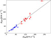 |
Fig. B.1. Comparison of Hα and [O III] velocity dispersion for our multicomponent fitting. Blue and red symbols represent narrow an broad Gaussian components. The solid gray line represents the unitary relationship. |
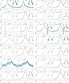 |
Fig. B.2. Single Gaussian vs. multi-Gaussian line fitting. For each panel, we show the single-component (left) and multicomponent (right) model of [O III] of each galaxy. Insets, colors, and symbols are the same as in Fig. 2 |
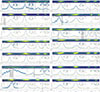 |
Fig. B.3. Summary of the multi-Gaussian fitting of Hβ, [O III] λ4959Å, and S II for the entire sample. Top: 2D spectra, with the y-axis in pixel units. Center: Gaussian fits for Hβ (left), [O III]λ4959Å (center), and S II (right). Bottom: Residuals of the fit. The peak emission of each line normalizes the flux. Spectra are shown in light blue ("Data"). The blue shadow represents the variance spectrum. The black line indicates the fit. The dashed lines show the different fitted components. The yellow line represents the continuum. Gray shadows are flagged regions excluded from fits. Insets that zoom in onto the faint line wings are included in the upper-right corner of each plot. |
All Tables
All Figures
|
Fig. 1. Top: 2D spectrum of SDSS143417 around the Hα[N II] region, with gray contours tracing flux levels and blue crosses marking the positions used for Gaussian fitting. Bottom: 1D spectra extracted with different apertures: the ESO pipeline, 30 px/side, including both knots (blue), IRAF/apall, 5 px centered on the brightest knot (orange), and IRAF/apall, with asymmetric aperture sampling the secondary knot (green). Vertical dashed lines indicate the wavelength ranges where the 2D contours reveal asymmetries, serving as guides to identify additional kinematic components. |
| In the text | |
|
Fig. 2. Multi-Gaussian fitting of bright emission lines for the galaxies in our sample. Top: 2D spectra, with the y-axis in pixel units. Center: Gaussian fits of [O III]λ5007Å(left) and Hα (right). Bottom: Fit residuals. The flux axis is normalized to the peak emission of each line. Spectra are shown in light blue (labeled “Data”). The blue shadow represents the variance spectrum. The black line models the fit. The dashed lines show the different fitted components. Gray shadows are flagged regions excluded from fits. The yellow line represents the continuum. Insets that zoom in onto the faint line wings are included in the upper-right corner of each plot. |
| In the text | |
|
Fig. 3. L − σ relationship. The blue and red circles correspond to the narrow and broad components of our sample of LBA galaxies, respectively. Gray symbols are Giant HII regions and H II galaxies at 0 < z < 2.33 from Terlevich et al. (2015). |
| In the text | |
|
Fig. 4. Classic diagnostic diagrams based on emission line ratios (Baldwin et al. 1981; Veilleux & Osterbrock 1987): [O III]λ5007/Hβ vs. [NII]λ6584/Hα (top) and [O III]λ5007/ Hβ vs. [S II]λλ6716.6731/Hα (bottom). Symbols show the emission-line–integrated fluxes (gray squares) and narrow (blue circles) and broad (red circles) Gaussian components for each galaxy. The gray dots correspond to the SDSS-DR7 MPA-JHU galaxy sample from Pérez-Montero et al. (2021). Regions of different excitation mechanisms are labeled and established by the theoretical and empirical demarcation lines of Kewley et al.; Kewley et al. (2001; 2006, dashed black), Kauffmann et al. (2003, dashed gray), and Schawinski et al. (2007), solid brown). |
| In the text | |
|
Fig. 5. Outflow mass loading factor as a function of the stellar mass of galaxies (left) and stellar mass outflow rate as a function of SFR surface density (right). Our LBAs are shown as red squares. Green and black circles are LBGs at z ∼ 1.4 − 3.8 from Weldon et al. (2024) and Llerena et al. (2023), respectively, while purple stars are mean-weighted averages from stacks of star-forming galaxies at z ∼ 2.1 from Concas et al. (2022). Gray and blue crosses are low-mass star-forming galaxies at z ∼ 3 − 9 observed with JWST/NIRSpec R = 2700 spectroscopy from Carniani et al. (2024) and Saldana-Lopez et al. (2025), respectively. The green crosses are the results from Xu et al. (2025b) for galaxies at z ∼ 3 − 9. Yellow stars are local dwarf galaxies from Marasco et al. (2023). Light blue squares indicate local dwarf galaxies from McQuinn et al. (2019). Dashed red lines are rescaled relations from Ilustris-TNG simulations of Nelson et al. (2019), and dashed black lines are from FIRE-2 simulations of Pandya et al. (2021). |
| In the text | |
|
Fig. B.1. Comparison of Hα and [O III] velocity dispersion for our multicomponent fitting. Blue and red symbols represent narrow an broad Gaussian components. The solid gray line represents the unitary relationship. |
| In the text | |
|
Fig. B.2. Single Gaussian vs. multi-Gaussian line fitting. For each panel, we show the single-component (left) and multicomponent (right) model of [O III] of each galaxy. Insets, colors, and symbols are the same as in Fig. 2 |
| In the text | |
|
Fig. B.3. Summary of the multi-Gaussian fitting of Hβ, [O III] λ4959Å, and S II for the entire sample. Top: 2D spectra, with the y-axis in pixel units. Center: Gaussian fits for Hβ (left), [O III]λ4959Å (center), and S II (right). Bottom: Residuals of the fit. The peak emission of each line normalizes the flux. Spectra are shown in light blue ("Data"). The blue shadow represents the variance spectrum. The black line indicates the fit. The dashed lines show the different fitted components. The yellow line represents the continuum. Gray shadows are flagged regions excluded from fits. Insets that zoom in onto the faint line wings are included in the upper-right corner of each plot. |
| In the text | |
Current usage metrics show cumulative count of Article Views (full-text article views including HTML views, PDF and ePub downloads, according to the available data) and Abstracts Views on Vision4Press platform.
Data correspond to usage on the plateform after 2015. The current usage metrics is available 48-96 hours after online publication and is updated daily on week days.
Initial download of the metrics may take a while.