| Issue |
A&A
Volume 707, March 2026
|
|
|---|---|---|
| Article Number | A136 | |
| Number of page(s) | 19 | |
| Section | Extragalactic astronomy | |
| DOI | https://doi.org/10.1051/0004-6361/202556612 | |
| Published online | 03 March 2026 | |
A long-term multiwavelength study of the flat spectrum radio quasar OP 313
1
Università di Trento, Via Sommarive 14 I-38123 Trento, Italy
2
Dipartimento di Fisica “M. Merlin” dell’Università e del Politecnico di Bari Via Amendola 173 I-70126 Bari, Italy
3
Istituto Nazionale di Fisica Nucleare, Sezione di Bari I-70126 Bari, Italy
4
Department of Physics and Astronomy, University of Turku FI-20014 Turku, Finland
5
Department of Astronomy, University of Geneva Chemin Pegasi 51 1290 Versoix, Switzerland
6
Istituto di Radioastronomia – INAF Via Piero Gobetti 101 I-40129 Bologna, Italy
7
Instituto de Astrofísica de Andalucía-CSIC, Glorieta de la Astronomia E-18008 Granada, Spain
8
Section of Astrophysics, Astronomy & Mechanics – Department of Physics, National and Kapodistrian University of Athens Panepistimiopolis Zografos 15784, Greece
9
Istituto Nazionale di Fisica Nucleare, Sezione di Roma “Tor Vergata” I-00133 Roma, Italy
10
ASI Space Science Data Center Via del Politecnico I-00133 Roma, Italy
11
Sapienza Università di Roma – Dipartimento di Fisica P.le A. Moro 00185 Roma, Italy
12
Finnish Centre for Astronomy with ESO University of Turku, Finland
13
Department of Fundamental Physics, University of Salamanca Plaza de la Merced s/n E-37008 Salamanca, Spain
14
Center for Astrophysics | Harvard & Smithsonian 60 Garden Street Cambridge MA 02138, USA
15
Institute for Astrophysical Research, Boston University 725 Commonwealth Ave. Boston MA 02215, USA
16
Max-Planck-Institut für Radioastronomie Auf dem Hügel 69 D-53121 Bonn, Germany
17
Aalto University Metsähovi Radio Observatory Metsähovintie 114 02540 Kylmälä, Finland
18
Aalto University Department of Electronics and Nanoengineering P.O. Box 15490 FI-00076 Aalto, Finland
19
Institut de Radiostronomie Millimétrique, Avenida Divina Pastora 7 Local 20 E–18012 Granada, Spain
★ Corresponding authors: This email address is being protected from spambots. You need JavaScript enabled to view it.
, This email address is being protected from spambots. You need JavaScript enabled to view it.
Received:
26
July
2025
Accepted:
11
January
2026
Abstract
Context. The flat spectrum radio quasar OP 313, is a high-redshift (z = 0.997) blazar that entered an intense γ-ray active phase from November 2023 to March 2024, as observed by the as observed by the Large Area Telescope (LAT) on board the Fermi Gamma-ray Space Telescope.
Aims. We present a multiwavelength analysis covering 15 years of data, from August 2008 to March 2024, to contextualize this period of extreme γ-ray activity within the long-term emission of the source.
Methods. We analyzed a long-term, comprehensive, multiwavelength dataset from different facilities and projects from radio to γ rays. We identified the seven most intense γ-ray flaring periods and performed a kinematic analysis of Very Long Baseline Array (VLBA) data to determine whether new jet components emerged before or during these flares. For two of these flaring periods, we performed the modeling of the spectral energy distribution (SED).
Results. The VLBA-BU-BLAZAR and MOJAVE datasets reveal a new jet component appearing in both visibility datasets prior to the onset of one of the strongest γ-ray flares. By comparing the timing of the VLBA-BU-BLAZAR knots’ ejection with the γ-ray flaring periods, we constrained the setup of the SED modeling. We also found that the first γ-ray flaring period is less Compton-dominated than the others.
Conclusions. Our results suggest that the recent activity of OP 313, is triggered by new jet components emerging from the core and interacting with a standing shock. The γ-ray emission likely arises from dusty torus photons upscattered via inverse Compton (IC) by relativistic jet electrons. The SED modeling indicates that this component is less dominant during the first γ-ray flaring period than the later ones.
Key words: radiation mechanisms: non-thermal / galaxies: active / galaxies: individual: OP 313 / gamma rays: general / X-rays: galaxies
© The Authors 2026
 Open Access article, published by EDP Sciences, under the terms of the Creative Commons Attribution License (https://creativecommons.org/licenses/by/4.0), which permits unrestricted use, distribution, and reproduction in any medium, provided the original work is properly cited.
This article is published in open access under the Subscribe to Open model. This email address is being protected from spambots. You need JavaScript enabled to view it. to support open access publication.
1. Introduction
Relativistic jets launched by active galactic nuclei (AGNs) are among the most energetic phenomena in the Universe and play a fundamental role in regulating galaxy evolution via feedback processes (Blandford et al. 2019). Blazars are a subclass of AGNs with their relativistic jet directed toward us. They are classified into two categories: flat spectrum radio quasars (FSRQs) and BL Lacs (BLLs). FSRQs exhibit strong and broad optical emission lines and high bolometric luminosities (Sambruna et al. 1996). They often display signs of thermal emission related to the accretion disk in their optical/UV spectra (Smith et al. 1986).
On the other hand, BLLs show weak optical lines and lower bolometric luminosities than FSRQs. Both categories exhibit extremely variable emission across the entire electromagnetic spectrum, on timescales ranging from months to minutes in the GeV and TeV bands (Aharonian et al. 2007; Ackermann et al. 2016). The physical mechanisms driving their variability remain unclear. Emission variability at different timescales may arise from distinct processes occurring in different regions within the AGNs. The detection of high-energy (HE, 0.1 − 100 GeV) and very high-energy (VHE, ≥100 GeV) emission from FSRQs suggests an origin further out in the jet, where the absorption of γ rays by external radiation fields, such as from the broad-line region (BLR), is reduced (e.g., Donea & Protheroe 2003).
The spectral energy distribution (SED) of blazars shows two peaks. The low-energy bump extends from the radio to the soft X-ray band and is interpreted as synchrotron emission produced by highly relativistic electrons within the jet. The HE bump extends up to γ-ray energies and its origin is still debated. In leptonic models, this bump originates from relativistic electrons in the jet upscattering low-energy photons through the inverse Compton process. Primarily, the low-energy photon field is provided by the synchrotron radiation within the jet, in a process known as synchrotron self-Compton (SSC, see, e.g., Inoue & Takahara 1996). In addition, low-energy seed photons from regions external to the jet, such as the accretion disk, the BLR, and the dusty torus (DT), can be upscattered via External inverse Compton (EC, see Dermer & Schlickeiser 1993; Dermer et al. 2009). In lepto-hadronic models, the interactions between relativistic protons and low-energy photon fields produce HE secondary particles, including γ rays and neutrinos (e.g., Kelner & Aharonian 2008; Rodrigues et al. 2021).
Indeed, blazars play a crucial role in multifrequency and multimessenger astrophysics, and some of them have been proposed as astrophysical neutrino sources (IceCube Collaboration 2018; Garrappa et al. 2019; IceCube Collaboration 2022). Nonetheless, both leptonic and lepto-hadronic models are usually capable of reproducing the observed emission from blazars (e.g., Mannheim & Biermann 1992; Aharonian 2000; Mücke & Protheroe 2001; Mücke et al. 2003; Böttcher et al. 2013).
OP 313, also known as B2 1308+326, is a FSRQ at a redshift of z = 0.997 (Schneider et al. 2010) and coordinates RA = 197.619433 deg and Dec = 32.345495 deg (Xu et al. 2019). Several observational campaigns targeting this source have been performed in the past due to its variability and uncertain classification (e.g., Britzen et al. 2017). In Stickel et al. (1991), OP 313, was classified as a BLL due to its nearly featureless optical spectrum (Wills & Wills 1979), high linear polarization in the optical band (> 3%, Jannuzi et al. 1993), and extreme optical variability (Angel & Stockman 1980). Nevertheless, based on very long base line interferometry (VLBI) measurements, Gabuzda et al. (1993) reported polarized emission from the inner jet of OP 313 with a position angle orthogonal to the jet direction and consequently identified the object as a FSRQ. Watson et al. (2000) observed OP 313, from radio to X-rays and suggested that it may be either a transitional blazar or a gravitationally microlensed quasar.
The Large Area Telescope (LAT) on board the Fermi Gamma-Ray Space Telescope detected flaring activity from OP 313, for the first time in April 2014, with an average γ-ray flux above 100 MeV of (1.1 ± 0.2)×10−6 ph/cm2s1 (Buson 2014). Two Astronomer’s Telegrams (ATels) were published in 2021 and 2022 (Mangal 2021; Garrappa 2022), reporting periods of re-enhanced activity from the source. OP 313, entered the phase of its highest activity in HE γ rays, as detected by the Fermi-LAT, on 22 November 2023.
The first peak of activity was reached on 24 November 2023 with an average γ-ray flux at energies above 100 MeV of (1.8 ± 0.2)×10−6 photons/cm2s, approximately 40 times larger than the flux reported in the fourth Fermi Large Area Telescope (4FGL) catalog (2.4 × 10⁻⁹ photons/cm2s from 0.1−100 GeV Abdollahi et al. 2020, 2022). Additionally, the photon index was significantly harder (1.80 ± 0.06) than the 4FGL catalog value of 2.34 ± 0.02. This flare led the Fermi-LAT Collaboration to publish an ATel on the 2023 high-state activity of the source (Bartolini et al. 2023). During this high state, VHE γ-ray emission from OP 313, was detected for the first time in December 2023 by the first prototype of the Large-Sized Telescope (LST-1) of the Cherenkov Telescope Array Observatory (CTAO), located on the island of La Palma (Cortina 2023).
This detection made OP 313, the most distant quasar detected at VHE γ rays so far. Another major flare from this source was detected on 27 February 2024, leading to the highest flux ever detected by the LAT for OP 313: (3.1 ± 0.4)×10−6 photons/cm2s, 60 times larger than the flux reported in the 4FGL catalog, with a photon index of 1.81 ± 0.09. This detection was reported in another ATel by the LAT collaboration (Bartolini 2024).
Given that OP 313 exhibited persistent high-state activity since 2022, following more than a decade of quiescence, we analyzed 15 years of data from radio to HE γ rays to unveil the mechanisms responsible for the observed flares. We note that the detailed study of the VHE emission period is not included in this paper, but it will be investigated in an upcoming publication by the MAGIC and LST Collaborations.
In Section 2, we present the multiwavelength dataset the analyses performed in each energy band. In Section 3, we present the 15-year-long multiwavelength light curve and identify the most relevant γ-ray flares covering the period from January 2022 to March 2024. In addition, we present and model the broadband SEDs collected during two of the highest flaring activity periods. Furthermore, we investigate the jet kinematics using an extensive Very Long Baseline Array (VLBA) dataset at 15 GHz and 43 GHz, as well as the correlation between the optical and γ-ray light curves. We summarize the main results and present our conclusions in Section 4.
2. Multiwavelength data
This section presents the multiwavelength (MWL) dataset employed for the investigation of OP 313, across the following energy bands: the radio band from 2.64 GHz to 353 GHz, the optical/UV bands from 170 to 690 nm, the X-ray band from 0.3 to 10 keV and the γ-ray one from 20 to 300 GeV. Table 1 summarizes the facilities whose data have been included in this work, as well as the time span of the observations.
Instruments whose datasets have been included for the long-term MWL analysis of OP 313.
2.1. Fermi-LAT data
The LAT is an imaging, wide field-of-view (FoV), pair-conversion γ-ray telescope covering an energy range from below 20 MeV to more than 300 GeV (Atwood et al. 2009). We analyzed 15 years of Pass 8 data (Atwood et al. 2013; Bruel et al. 2018) collected by the LAT using the standard LAT ScienceTools1 v2.2 and the fermipy (Wood et al. 2018) v1.1 Python package. We used the P8R3_SOURCE_V3 instrument response functions, the Third Data Release 4FGL-DR3 (Abdollahi et al. 2022), and the Galactic and the isotropic diffuse gamma-ray emission models provided by the standard templates gll_iem_v07.fits and iso_P8R3_SOURCE_V3_v1.txt2. We analyzed photon events with reconstructed energy between 100 MeV and 300 GeV, selecting a region of interest (ROI) of 15 × 15 deg2 centered on OP 313, and applying a standard quality cut (‘DATA_QUAL> 0&&LAT_CONFIG= = 1’). Furthermore, a zenith angle cut of 90 deg was used to reduce the contamination from the Earth limb.
We modeled the spectrum of OP 313, with a log-parabola function3. We performed a maximum-likelihood analysis and defined the test statistic (TS) of OP 313, as TS = 2(log L1 − log L0), L1 and L0 being the likelihood of the data for a model with and without a point source located at the position of OP 313, respectively. In the fit, we left free to vary the parameters of the OP 313, spectral model, as well as the normalizations of all sources with TS ≥ 25 located within 5 deg from OP 313, and the normalizations of the Galactic and isotropic diffuse components.
By using the adaptive binning algorithm described in Lott et al. (2012), we computed a sequence of time bins spanning from 2008 to 2024 with a fixed relative uncertainty of 0.2 for the reconstructed OP 313, flux. The light curve computed using these adaptive bins is shown in Figure 1. Moreover, we identified statistically significant variations of the OP 313, flux using the Bayesian Blocks algorithm (Scargle et al. 2013), as implemented in astropy4.
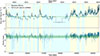 |
Fig. 1. Top: 15-year Fermi-LAT light curve of OP 313, divided into quiescent (blue) and flaring (yellow) states. The green line shows the time-weighted average flux of 4.93 × 10⁻⁸ photons/cm2s computed between 9 December 2014 and 9 August 2018. Bottom: Fermi-LAT photon index over the same 15-year period. The green line shows the average photon index computed between 9 December 2014 and 9 August 2018 (Γ = 2.39), with the green band indicating its corresponding 1σ uncertainty. The red vertical bands highlight the period in which LST-1 detected OP 313. |
The OP 313 flaring activity and quiescent states were determined following the approach in Rodrigues et al. (2021). As a proxy for the quiescent state, we considered the time-weighted average flux over the low-activity period spanning from 9 December 2014 to 9 August 2018. The bayesian blocks with fluxes above 4.93 × 10⁻⁸ photons/cm2s are identified as flaring states, whereas those below this threshold represent the quiescent ones. These are shown in yellow and blue in Figure 1, respectively. The red band in Figure 1 represents the period in which the LST-1 detected OP 313. The source has remained in a flaring state since late 2021. Figure 1 shows that the photon index from the beginning of 2022 is generally harder than the average measured between 9 December 2014 and 9 August 2018 (Γ = 2.39 ± 0.25, in green).
2.2. Neil Gehrels Swift Observatory data
The Neil Gehrels Swift Observatory (Swift) (Gehrels et al. 2004) mission is a fast-repositioning, multiwavelength satellite primarily designed for gamma-ray burst (GRB) studies. Its equipped with three instruments: the Burst Alert Telescope (BAT, Barthelmy et al. 2005), sensitive to the 15 − 350 keV range, the X-Ray Telescope (XRT, Burrows et al. 2005), operating in the 0.2 − 10 keV band, and the UV/Optical Telescope (UVOT, Roming et al. 2005), covering the 190 − 600 nm wavelengths.
We analyzed the Swift-XRT observations of OP 313, from 20 August 2008 to 9 March 2024. We used the spectral fitting package XSPEC v12.13.1 (Arnaud 1996) and the python package PyXspec v2.1.4 available in the HEASOFT software v.6.33.1, together with the calibration database (CALDB) v20220331. We modeled the observed XRT spectra using a phabs*zpowerlw function5. The phabs term accounts for the Galactic extinction, and the hydrogen column density was fixed to NH = 1.23 × 1020 cm−26.
Conversely, the zpowerlw model is defined as:
![Mathematical equation: $$ \begin{aligned} \frac{\mathrm{d}N}{\mathrm{d}E} = N_{0} [E(1+z)]^{\alpha }, \end{aligned} $$](/articles/aa/full_html/2026/03/aa56612-25/aa56612-25-eq1.gif) (1)
(1)
where N0 is the normalization in units of photons/keV/cm2/s, E is the energy in keV units, z is the redshift, and α is the photon index. For each XRT exposure, the intrinsic X-ray SED of OP 313, was reconstructed by correcting the observed spectral points for the Galactic extinction effects, using the procedure presented in Abe et al. (2025).
The Swift-UVOT data from the same period were processed and analyzed using the uvotimsum and uvotsource tasks in HEASOFT. The available UVOT observations were performed using the optical v, b, u and UV w1, m2, w2 photometric filters. The source counts were extracted from a circular source region of 5 arcsec radius centered at the OP 313, position, whereas a circular nearby region of 20 arcsec radius devoid of sources was used to derive the background counts. We accounted for the Galactic extinction using E(B − V) = 0.0115 ± 0.0005 (Schlafly & Finkbeiner 2011).
2.3. Optical
The long-term optical light curve was assembled by using the photometric data from several all-sky surveys and dedicated blazar monitoring programs: Zwicky Transient Facility7 (ZTF, Bellm et al. 2018), Catalina Real-Time Transient Survey8 (CRTS, Drake et al. 2009), Irsa’s Image and Spectrum Server9 (ATLAS), Katzman Automatic Imaging Telescope10 (KAIT, Filippenko et al. 2001) at the Lick Observatory and the Tuorla blazar monitoring program11 (Nilsson et al. 2018). For each of these facilities, the photometric filters included in this work are reported in Table 1.
The survey datasets have been extracted from the corresponding databases, while the dedicated observations of this source from the Tuorla blazar monitoring were analyzed using the standard procedures of differential photometry, with a semi-automatic pipeline (e.g., Nilsson et al. 2018) and an aperture of 5 arcsec. The optical data from all the facilities were combined following the prescriptions of Kouch et al. (2024). Data from simultaneous and quasi-simultaneous nights were used to estimate the shifts between different observatories, using the Tuorla blazar monitoring data as reference point.
2.4. Metsähovi
We included 37 GHz observations made with the 13.7 m diameter Metsähovi radio telescope (see Table 1). The detection limit of the telescope at 37 GHz is on the order of 0.2 Jy under optimal conditions. Data points with a signal-to-noise ratio < 4 are handled as non-detections. The flux density scale is set by the observations of DR 21, whereas NGC 7027, 3C 274, and 3C 84 are used as secondary calibrators. A detailed description of the data reduction and analysis is given in Teräsranta et al. (1998). The error estimate in the flux density includes the contribution from the root mean square (rms) and the uncertainty of the absolute calibration.
2.5. F-GAMMA, QUIVER and SMAPOL
The Effelsberg 100-m Radio Telescope measured the total flux density of OP 313 within the framework of the F-GAMMA (FERMI-GST AGN Multi-frequency Monitoring Alliance) and QUIVER (Monitoring the Stokes Q, U, I and V Emission of AGN jets in Radio) monitoring programs. F-GAMMA followed the radio variability of several γ-ray loud blazars between 2007 and 2015. A complete description of the project and the dataset collected by the Effelsberg telescope can be found in Fuhrmann et al. (2016) and Angelakis et al. (2019). F-GAMMA was followed by the QUIVER monitoring program, which monitors the total flux density and polarization evolution of a subset of the F-GAMMA sources, including OP 313 on a fortnightly basis since June 2015.
The F-GAMMA and QUIVER observations are performed at several radio bands (depending on receiver availability and weather conditions) from 2.6 GHz to 44 GHz (11 cm to 7 mm wavelength) using nine receivers located at the secondary focus of the 100-m Radio Telescope. The polarized intensity, position angle, and polarization percentage were derived from the Stokes I, Q, and U cross-scans. The total flux was computed using the calibrators 3C 286, 3C 48 and NGC 7027 (e.g., Myserlis et al. 2018; Kraus et al. 2003). In this paper, we used the F-GAMMA data from 22 August 2008 to 1 June 2014, and the QUIVER data from 13 November 2023 to 30 March 2024.
The Submillimeter Array (SMA) (Ho et al. 2004) was used to obtain total flux at 1.3 mm (225 GHz) within the framework of two complementary programs: the standard SMA flux monitoring campaign (Gurwell et al. 2007) and the recent SMAPOL (SMA Monitoring of AGNs with POLarization) program. SMAPOL follows the evolution of forty gamma-ray loud blazars, including OP 313, since June 2022 on a fortnightly cadence. We employed MWC 349 A, Callisto, Uranus, Neptune, and Ceres for the total flux calibration according to their visibility. The SMA data used in this work span from 13 September 2008 to 10 March 2024, and include observations from both the flux monitoring and SMAPOL programs at 225, 273 and 350 GHz.
2.6. VLBA data
The VLBA-BU-BLAZAR12 and Monitoring Of Jets in Active galactic nuclei with VLBA Experiments (MOJAVE)13 monitoring programs consist of monthly VLBA observations of blazars and radio galaxies. The MOJAVE data archive consists of nearly ten thousand total density fluxes VLBA observations at 15 GHz (2 cm) of over 500 AGN dating back to 1994 (Lister et al. 2021). Instead, the VLBA-BU-BLAZAR monitoring program observes a sample of AGN detected in the γ-ray band at 43 GHz (7 mm) and 86 GHz (3.5 mm) (Jorstad et al. 2017; Weaver et al. 2022). The available data for OP 313 are taken at 43 GHz. We included VLBA-BU-BLAZAR data from 1 April 2009 to 22 March 2024 and data from 7 January 2009 to 7 April 2024 from the MOJAVE project.
We modeled the sky brightness distributions in the (u, v) visibility plane. We modeled the visibilities of OP 313 with a series of circular Gaussian components using the modelfit task in the Difmap v2.5o software package (Shepherd 1997). We refer to these Gaussian components using the term “knots”, which are usually compact features of enhanced brightness in the jet. We started with a single circular Gaussian component approximating the brightness distribution of the core, which is typically the brightest feature on the map located close to the base of the jet. Then knots were iteratively added at the locations of bright features. For every knot that we added, we used the modelfit task to determine the best-fit parameters of the knot, according to a χ2 test. The fit procedure was iterated until the addition of a new knot did not significantly improve the χ2 value. The model of a previous epoch was used as the starting model for the next epoch, since we assume that the jet does not change drastically on monthly timescales (Weaver et al. 2022).
3. Results
This section presents the main results of the analyses performed on the multiwavelength dataset.
3.1. Multiwavelength light curves of OP 313
Figure 2 shows the radio to γ-rays light curve from 4 August 2008, to 9 March 2024 (MJD 54682.7–60378.0). Starting in 2022, the source shows a systematic increase in flux across the γ-ray, X-ray, and optical/UV bands. Before this period, its activity was limited to small flaring episodes, marginally visible in the γ-ray light curve. Instead, the radio light curves show variability over the 15 years. Across all radio frequencies, a common trend emerges: the source was in a high-flux state from the beginning of our analysis in 2008, followed by a gradual decline until 2019, after which the flux began to increase once more (see more details in Section 3.4).
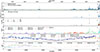 |
Fig. 2. Multiwavelength light curve of OP 313. The red vertical band indicates the period when LST-1 detected OP 313. a: Fermi-LAT light curve at E > 100 MeV. b: Swift-XRT X-ray light curve from 0.3 keV to 10 keV. c: Swift-UVOT light curve in the optical/UV bands. d: Optical light curve from several facilities and filters: CRTS V-filter (cV), KAIT R-filter (kR), Tuorla R-filter (tR), ATLAS o (Ao) and c-filters (Ac), and Palomar ZTF g, r, and i-filters (zG, zR, and zI). The label zGzR refers to ZTF observations using both g and r filters. e: Radio Single Dish FERMI-GST AGN Multi-frequency Monitoring Alliance (F-GAMMA) light curves above 15 GHz, Submillimeter Array (SMA) data at 225, 273 and 350 GHz, including SMAPOL data at 225 GHz light curves, Metsähovi at 37 GHz and VLBA-BU-BLAZAR at 43 GHz light curves. f: Radio Single Dish F-GAMMA light curves below 15 GHz and MOJAVE VLBA light curve. |
3.2. Selection of the flaring periods of interest
In Figure 1, the source began a continuous flaring phase at the end of 2021. Particularly noteworthy is the multiwavelength flaring activity, spanning from γ-rays to optical frequencies, which started in 2022 and persisted until the end of this study. Figure 3 presents the γ-ray and optical light curves from 1 January 2022 to 9 March 2024, showing a good correlation between the two datasets, despite the limited optical coverage during the flaring episode reported in Bartolini et al. (2023). Further discussion on the γ-ray–optical correlation is provided in Section 3.2.3.
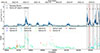 |
Fig. 3. Fermi-LAT (top) and optical (bottom) light curves from 1 January 2022 to 9 March 2024. The dashed black lines indicate the brightest γ-ray flaring periods. The fourth and sixth flaring periods are not between the brightest but are located in time between the ATels Bartolini et al. (2023) and Bartolini (2024). The red vertical bands indicate the period when LST-1 detected OP 313. |
The highest γ-ray flaring episodes within this time interval were identified by selecting the Bayesian blocks with the highest average flux. Seven distinct flaring episodes were found, marked with black dashed lines in Figure 3. The fourth and sixth flaring periods are not among the brightest, but they occurred temporally between the ATels Bartolini et al. (2023) and Bartolini (2024). We decided to include them, given our interest in unveiling the mechanisms responsible for the intense flaring activity. Table 2 shows: (1) ID of the flaring period, (2) flaring period in MJD, (3) flux peak and its error, (4) photon index corresponding to the flux peak, (5) fluence in the flaring period, defined as the time-integrated flux. We note that although Flare 3 coincides with the detection of OP 313 at energies above 250 GeV, it is not the brightest among the identified events, but it exhibits one of the hardest spectral indices.
Flaring periods of OP 313 starting from January 2022.
3.2.1. Search for hysteresis patterns
The hysteresis pattern (e.g., Kirk et al. 1998) is a loop-like structure that provides insight into the particle acceleration and cooling mechanisms occurring within the blazar’s jet. There are two different kinds of hysteresis patterns:
-
the more common clockwise pattern, indicating the spectral slope is dominated by synchrotron cooling (Tashiro & Makishima 1995);
-
the rare counterclockwise pattern, which suggests that the cooling and acceleration rates are comparable and the flaring event propagates from lower to higher energies.
As shown in Figure 1, the γ-ray photon statistics obtained with Fermi-LAT is large enough to investigate possible hysteresis patterns during the flaring periods defined in Section 3.2. We realized the hysteresis plots n which the spectral index is plotted on the y-axis as a function of the flux on the x-axis.
Visual inspection of the plots (Figure 4a) suggests for the 1st flare a hint of anti-clockwise pattern arising on 4 July 2022. Instead, hints of clockwise hysteresis patterns were found for the second, in Figure 4c, and fifth flaring periods, in Figure 4b. This means that these flaring periods are dominated by the cooling. There are no hints of hysteresis patterns for the rest of the periods.
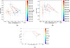 |
Fig. 4. (a) Hysteresis pattern of the first flaring period (2 July 2022 – 15 July 2022). The dashed gray line is included to guide the eye in identifying the temporal sequence of the points. (b) Hysteresis pattern of the fifth flaring period (30 January 2024 – 8 February 2024). (c) Hysteresis pattern of the second flaring period (20 November 2023 – 29 November 2023). |
Evaluating statistical significance of hysteresis patterns is non trivial, but one possible test is to bin the data differently. In Appendix A, Figures A.1a, A.1b and A.1c present the hysteresis patterns for first, second, and fifth flaring periods, using the average photon index computed in 2-day-long time bins. In this case, the number of data points is smaller as well as the associated uncertainties. The resulting hints of hysteresis pattern are anti-clockwise for the first and fifth flaring periods and clockwise for the second flaring period. Therefore, we conclude that our search for hysteresis patterns was inconclusive even for these extremely bright flares.
3.2.2. Compton dominance
Figure 3 presents the flaring activity of OP 313 from 1 January 2022, to 9 March 2025. The first optical flaring period is stronger than its γ-ray counterpart, whereas the opposite trend is observed for the subsequent ones. This disparity between flaring periods across various wavelengths suggests a shift in the origin of the seed photons responsible for Comptonization. For FSRQs such as OP 313, the soft seed photons for external Compton scattering are expected to originate outside the jet (Nalewajko & Gupta 2017). Hence, investigating the relative variability between the two SEDs peaks helps to constrain the nature and location of the external photon field.
In this study, we compared the SEDs of selected flaring periods to investigate differences in the relative intensities of their two peaks. The heights of these peaks in a blazar SED are directly connected to the Comptonization processes. When the synchrotron and HE peaks have comparable amplitude, the jet is moderately magnetized, and synchrotron self-Compton (SSC) dominates the HE emission (Finke 2013; Potter & Cotter 2013). When the HE peak significantly exceeds the synchrotron peak, the Compton dominance is high, and external Compton (EC) scattering becomes the primary radiative mechanism. A high synchrotron luminosity (Lsyn > 1047 erg/s, Janiak et al. 2015) implies highly magnetized emitting region in the jet and efficient synchrotron cooling (Janiak et al. 2015). Figure 5 shows the SEDs of the first and fifth flaring periods, as well as a quiescent period going from 1 March 2016 to 1 January 2018. The first flaring period SED exhibits peaks of comparable heights, whereas the fifth presents peaks at different heights. This indicates low Compton dominance during the first flaring period and a more Compton-dominated scenario in the fifth. All the flaring periods from November 2023 to March 2024 exhibit enhanced Compton dominance. A lower Compton dominance suggests that SSC emission is dominating over the EC, whereas a higher dominance is often interpreted as evidence for prevailing EC scattering (Sikora et al. 1994). In Section 3.5, for coherence, we discuss in detail the SED modeling study of these 2 flaring periods.
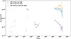 |
Fig. 5. SED of the first (2022), in orange, the fifth flaring periods (January 2024), in blue, and a quiescent period that goes from March 2016 to January 2018, in purple. The X-ray, UV, optical, and radio SED points correspond to the average flux values within each period at their respective frequencies. No Swift-XRT and UVOT data were available during the quiescent period. |
3.2.3. Multi-band correlation
Understanding blazar jet emission and its dynamics requires examining how changes in their physical properties drive variability across various frequencies (Mohana A et al. 2024). A cross-correlation approach effectively identifies plausible links across different blazar emission bands, distinguishes emission components in the jet, constrains the emission zone’s location, and differentiates between SSC and EC models (Liodakis et al. 2019).
The z-transformed Discrete Correlation Function (zDCF Alexander 1997) was employed to estimate the cross-correlation between the γ-ray and optical light curves (e.g., as in Abe et al. 2025). The zDCF evaluates the delay-dependent multi-band cross-correlations. This method is more sophisticated than the Discrete Correlation Function (DCF; Edelson 1988) because it uses equal-population binning and Fisher’s z-transform, and it is developed for sparse and unevenly sampled astronomical time series. A Python implementation of the original Fortran zDCF algorithm called the pyZDCF package (Jankov et al. 2022) was used to evaluate the zDCF. We investigated the cross-correlation between the optical and γ-ray datasets both in the long-term period (see Figure 2) and in the short-term period from 2022–2024 (see Figure 3). The zDCF evaluation was performed using bins of delay of 2, 3, and 4 days. For all the delay bin sizes we used, the zDCF showed a peak at a delay compatible with 0 days. For the long-term (short-term) period, the zDCF at zero delay was found to be equal to 0.8 (0.6, see Figure 6a).
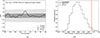 |
Fig. 6. (a) zDCF analysis on the short-term period of OP 313 optical and γ-ray light curves; and (b) distribution of the reconstructed zDCF at zero time-lag for 104 simulated uncorrelated γ-ray and optical light curves. The red line marks the reconstructed zDCF value with the observed OP 313 light curves in Figure 3. |
To perform the significance analysis of the observed light curves’ zDCF, we modeled the power spectral density (PSD) of each observed light curve using a power-law function PSD(ω) = Aω−β. We estimated a best-fit index value for the γ-ray light curve of βγ = 1.2, in agreement with Tarnopolski et al. (2020), whereas for the optical R-band light curve, we found βOPT = 1.2, which is comparable with the typical ranges reported in Nilsson et al. (2018) for blazars.
The significance of the observed zDCF peak was evaluated by generating 104 pairs of uncorrelated γ-ray and optical light curves with the same PSDs and flux distributions as the real ones. We used the DELCgen Python package (Connolly 2016) to generate the fake light curves population using the Emmanoulopoulos et al. (2013) (EM) method. We used the EM method because it also takes into account the distribution of the observed light curves’ fluxes, whereas the Timmer & König (1995) (T & K) method simulates light curves assuming the observed fluxes follow a Gaussian distribution.
These simulated pairs of light curves were used to derive the confidence bands of the zDCF under the hypothesis of non correlation. The 1σ and 3σ bands for the 2022–2024 period are shown in Figure 6a. In the bin of zero delay, we found the positive correlation with zero delay between the optical and γ-ray light curves to be significant above the 95% confidence level, corresponding to a confidence level of roughly 2σ (see Figure 6b). This correlation suggests a common origin for the flaring emission in the two bands, indicating that leptonic processes primarily dominate the γ-ray emission, though a subdominant hadronic contribution cannot be ruled out (Acharyya & Sadun 2023).
3.3. VLBA jet kinematics results
The VLBA analysis consisted of the analysis of data from the MOJAVE and VLBA-BU-BLAZAR programs. We identified new knots in the parsec-scale jet that may be responsible for the flaring activity observed in OP 313. To interpret these multiwavelength flaring events, we performed a kinematic analysis of the newly detected components.
3.3.1. MOJAVE VLBA analysis results
The jet components and corresponding kinematic parameters of OP 313 between 1995 and August 2019 have been previously presented in Lister et al. (2019, 2021). Since our long-term multiwavelength study extends to March 2024, we analyzed all the public visibilities up to 4 April 2024, which is the closest observation to 9 March, employing the procedure outlined in Section 2.6. The main outcomes of this analysis are:
-
The visibility modeling results obtained between August 2008 and August 2019 are in agreement with those reported in Lister et al. (2019, 2021). Hence, in Figure 7, the components and their distance from the core in this period are the same as reported in the literature;
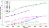
Fig. 7. Angular separation from the core versus time for Gaussian jet features of the MOJAVE data. Colored symbols indicate robust features for which kinematic fits were obtained. The 1σ positional errors on the individual points typically range from 10% of the FWHM restoring beam dimension for isolated compact features to 20%, represented as a black cross in the plot, of the FWHM for weak features (see e.g., Lister et al. 2009, 2019, 2021).
-
A new, well-defined jet component is first detected on 13 April 2021.
We employed the same approach as Lister et al. (2021) to determine if this new component is a robust cross-identification, checking whether the feature was present across at least five epochs, and considering the consistency of its sky position and flux density over time. The new component was named “Component 24” and is colored in red in Figure 7.
We analyzed the kinematics of all individual robust jet features, from August 2008 to April 2024, employing the method reported in Lister et al. (2021). We fit the sky positions of these features, as follows:
 (2)
(2)
 (3)
(3)
where tmid represents the midpoint between the first and last observation epochs of the component, μx and μy are the fit angular velocities in each sky direction, and  and
and  are the fit accelerations. The 1σ uncertainty on the position of the knots ranges from 10% of the full-width half maximum (FWHM) restoring beam dimension (a median reference value is 0.096 along the major axis of the restoring beam and 0.056 along its minor axis) for isolated compact features to 20% of the FWHM for weak features (around 0.19 along the major axis and 0.11 along the minor axis) (see e.g., Lister et al. 2009, 2019, 2021). The acceleration of the new “Component 24” could not be evaluated because it does not meet the requirement of being detected in at least ten epochs. Instead, “Component 20” corresponds to a static shock. To determine the proper motion vector modulus and apparent velocity in units of speed of light, we used the following equations:
 (4)
(4)
 (5)
(5)
where DA corresponds to the angular distance and z is the redshift of the source. Table B.1 in Appendix B presents the parameters derived from the fitting procedure, which characterize the kinematics of the jet components.
3.3.2. VLBA-BU-BLAZAR analysis results
The VLBA-BU-BLAZAR jet components and corresponding kinematic parameters of OP 313 between 2009 and 2018 have been presented in Jorstad et al. (2017) and Weaver et al. (2022). We analyzed the public visibilities up to 7 April 2024 employing the method reported in Section 2.6. The main outcomes of this analysis are:
-
The visibility modeling results obtained for the period between 2008 and 2018 are consistent with those presented in Jorstad et al. (2017) and Weaver et al. (2022). Hence, Figure 8 reproduces the components “A1”, “A2” and from “B1” to “B8”, along with their distances from the core as reported in the literature;
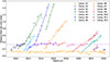
Fig. 8. Angular separation from the core versus time for Gaussian jet features of the VLBA-BU-BLAZAR (VLBA-BU-BLAZAR) data. Colored symbols indicate robust features for which kinematic fits were obtained. The 2 dashed lines in yellow and purple represent the static shocks’ mean distance from the core.
-
A new set of jet components arose starting from 2019, as shown in Figure 8.
The components’ flux and coordinates uncertainties were computed using the formalism described in Jorstad et al. (2017) and are presented in Table B.2. This formalism is based on an empirical relation between the uncertainties and the brightness temperatures of knots: Tb, obs = 7.5 × 10⁸S/a2 K, where Tb, obs is the brightness temperature of the knot in Kelvin, S is the flux density in Jy and a is the angular size in mas of the knot (e.g., Jorstad et al. 2005; Casadio et al. 2015; Weaver et al. 2022). The uncertainties are calculated as follows: the 1σ uncertainty on the x-axis is  , the uncertainty on the y-axis is σy ≈ 2σx, the flux uncertainty is
  and the angular size uncertainty is
  . We added a minimum positional error of 0.005 mas (related to the resolution of the observations) and a typical amplitude calibration error of 5% (Jorstad et al. 2017; Weaver et al. 2022) to σx and σy.
The kinematic properties of the jet components were derived following Weaver et al. (2022). Components detected in more than four epochs, exhibiting consistent positions and fluxes over time, were fit using the weighted least-squares implementation in the statsmodels package14 (Seabold & Perktold 2010). From the comparison between the χ2 obtained in the fitting process and  at a significance level of ζ = 0.05 values, we identified accelerating components (
 ), which required segmented fits representing distinct velocities along their motion. Accordingly, Table B.2, in Appendix B, lists some components with two angular proper motion and apparent speed entries for components fit with two segments. The derived jet structure and kinematic parameters are consistent with Jorstad et al. (2017) and Weaver et al. (2022). The parallel and perpendicular accelerations are given by:
  and
and  , where ⟨Θjet⟩= − 64.9 ± 4.7 is the average jet position angle for OP 313, (Weaver et al. 2022), describing the jet orientation on the sky plane, measured from north to east (Lister et al. 2009). Table B.2 reports the kinematic properties of the new components arising after 2018. Notably, “Component 24” appears consistent with the component “B9”, as both occupy similar distances from the core and exhibit comparable proper motion magnitudes and apparent speeds, both in red in Figures 7 and 8. Further observations are required to robustly confirm the identification of some of the later components, such as “B12”, which appears in only four epochs in our dataset, as well as others that emerged toward the end of our analysis. For more comprehensive details and information about later components, we refer the reader to Jorstad et al.’s forthcoming publication.
Doppler factor (δvar), Lorentz factor (Γ), and viewing angle (Θ0) of the new components detected from 2019 in VLBA-BU-BLAZAR visibilities.
3.3.3. Lorentz factor and viewing angle of jet components
Blazar jets are known for their extraordinarily fast variability, boosted emission, and apparent superluminal motion of jet components, due to relativistic processes that dominate the jet’s emission. These relativistic effects are quantified by Lorentz factor (Γ), the Doppler factor (δ), and viewing angle (Θ0), which is the angle between the jet axis and the line of sight to the observer (Hovatta et al. 2009). The apparent velocities of the new components were used to compute their corresponding Lorentz factors and viewing angles following the formalism of Jorstad et al. (2017) and Weaver et al. (2022):
 (6)
(6)
 (7)
(7)
where δvar is the variability Doppler factor and is defined as:
 (8)
(8)
where DGpc is the luminosity distance of OP 313 in Gpc, s = 1.6a is the diameter of a face-on disk with a being the angular size of the knot in mas, which is the FWHM of a Gaussian brightness distribution, and τvar = |1/k| is the variability timescale. The parameter k is obtained by fitting the flux decay of the knots with an exponential model ln(S(t)/S0) = k(t − tmax), where S is the flux density, S0 is the flux fit at tmax, and k is the slope (Weaver et al. 2022). Using this formalism, we computed the Doppler factor, Lorentz factor, and viewing angle for the new components, from “B9” to “B12”; the results are listed in Table 3. For the other components, these parameters are available in Weaver et al. (2022). The Doppler factors of the knots from “B9” to “B12” range between 8 and 15, while the Lorentz factors range between 7 and 13. These values are in agreement with the general trend for FSRQs reported in Hovatta et al. (2014) and Liodakis et al. (2018). Using the equation (7), the inferred viewing angles are between 2 and 7 deg. The accuracy for the component “B12” is limited due to its detection in only a few epochs. Future analysis of additional VLBA-BU-BLAZAR visibilities, as well as the upcoming paper from Jorstad et al. (in prep.), may improve these estimates.
Lorentz factor (Γvar) and viewing angle (Θ0) of the new components arisen from 2019 in the visibilities of the VLBA-BU-BLAZAR project.
Moreover, using the Doppler factor at 37 GHz  (Liodakis et al. 2021), we recalculated the viewing angle and Lorentz factor to be compared with the values obtained in (see Table 4). The results are broadly consistent with Table 3, except for “B12”, which has limited data.
Overall, the inferred values in Table 3 and in Table 4 for B9–B12 are consistent with the general trends for FSRQs, where δvar < 40 and Γvar ∼ 10 for FSRQ (Hovatta et al. 2014; Liodakis et al. 2018).
3.4. Search for the origin of the γ-ray flaring periods
In Figure 2, the radio flux was increasing until 2010 and then started rising again around 2019. Although the light curve suggests a possible long-term trend, previous studies of the radio variability of OP 313 using Metsähovi data from 1985 to 2023 show that no characteristic variability timescale can be well-established for this source (Kankkunen et al. 2025). Consequently, the flaring activity observed since 2022 cannot be associated with any well-defined periodic behavior (see Table 5).
Epoch of ejection T0 and epoch in which the knot encounters the static shock T1 for the new knots found in the VLBA-BU-BLAZAR data.
Figure 9 compares the LAT and MOJAVE total flux density light curves from 2018 to March 2024, suggesting a time delay between the two bands. This time lag was investigated for OP 313 in Kramarenko et al. (2022), who reported a delay of  days between γ-ray and radio. A positive time lag indicates that the γ-ray emission leads the radio emission, implying that the region responsible for the γ-ray flares is closer to the central engine than the radio-emitting region. The Kramarenko et al. (2022) time lag is smaller than the value we derived looking at the γ-ray and radio emissions between 2020 and 2021, shown in Figure 9, where we measured a delay of 201 ± 16 days by comparing the difference between the epochs where the radio and γ-ray emissions had a peak. Furthermore, Kramarenko et al. (2022) computed the distance between the γ-ray emission region and the central engine, taking the radio core opacity as the main source of the time lag. For OP 313, they found that the γ-ray emission region is located at
  pc (Kramarenko et al. 2022) from the central engine, beyond the BLR whose external radius is ≃0.1 pc (see Section 3.5 for the derivation of the BLR radius). This motivated us to foresee a photon field responsible for the EC in the dusty torus, outside the BLR.
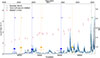 |
Fig. 9. Comparison between the Fermi-LAT data (in blue) with their Bayesian blocks (in black) and the total flux density of MOJAVE data at 15 GHz (in red). The dashed blue lines represent the time of ejections for different knots, found in the VLBA-BU-BLAZAR visibilities, and the blue lines are the corresponding errors, while the orange dashed lines represent the epochs when the knots encounter the standing shock “A1” with the corresponding errors. In green, the epoch in which “B12” was found. |
Moreover, Figure 9 shows with dashed colored lines the period in which the new knots “B9”–“B11” passed the radio core, in blue, and passed the static shock “A1”, in yellow. The green dashed line indicates the epoch when component “B12” was found. We followed the approach described in Weaver et al. (2022) to estimate the ejection epoch, T0, and the epoch when the knots encounter the static shock, T1. Hence, for each component, we used either the first ten observed epochs or, in the case of accelerating knots, the points belonging to the first kinematic segment. Linear fits to the x and y coordinates were extrapolated back to the core position (0, 0) and to the location of the stationary shock “A1”. This procedure provides the time of ejection along each coordinate, Tx0 and Ty0, and Tx1 and Ty1. Then the true time of ejection and its 1σ uncertainty are given by
 (9)
(9)
 (10)
(10)
where  and
and  are the 1σ propagated uncertainties on Tx0 and Ty0. The same equations were used to calculate T1 and σT1 substituting Tx0, σTx0, Ty0 and σTy0 with Tx1, σTx1, Ty1 and σTy1.
Component “B12” is detected over too few epochs to allow a reliable calculation of either the epoch of ejection or its interaction with the stationary shock. Based on Figure 9, we argue that the ejection of “B9” and “B10”, as well as their encounter with the static shock could be responsible for the flaring activity that occurred from 2019 to the beginning of 2020 (see Table 5). Since the knot “B9” could be consistent with Component 24 of the MOJAVE data, we calculated T0 and T1 using equations (9) and (10) also for Component 24. In this case, we considered component 20 as the first static shock encountered by the knot since its distance from the core and its trend are consistent with “A1”. The results are reported in Table 6. Similarly, the ejection and the shock interaction component “B11” could be responsible for the flaring activity from late 2021 through 2022. Hence, component “B12” and additional components that are still emerging could be responsible for all the flaring emissions from late 2023 to early 2024. In summary, we suggest that Flare 1 is associated with the interaction of “B11” with the standing shock, while Flare 2 to 7 could be linked to “B12”, for which more VLBA observations are needed. However, the timing suggests the flaring began when the knot was still within the core or even before it reached the core. This and the appearance of further new VLBA components will be analyzed in Jorstad et al. (in prep.).
Epoch of ejection T0 and epoch in which the knot encounters the static shock T1 for component 24.
3.5. SED modeling
Section 3.4 suggests a slightly different site for the flaring region within the jet for Flare 1 with respect to the flares from 2 to 7. Among these, the best sampled SED is the Flare 5 one, which is why we selected it for our Compton dominance analysis (see Section 3.2.2). In this section, we investigate whether we can model the spectral energy distributions of these two states.
For the modeling and fitting of the two radiative states of OP 313, we have used the JetSeT framework (Tramacere et al. 2009, 2011; Tramacere 2020). This is an open-source framework written in C/Python designed to simulate the radiative, accelerative processes, and adiabatic expansion occurring in relativistic jets and galactic objects, both beamed and unbeamed. This enables fitting numerical models to observational data, supporting the definition of complex numerical radiative scenarios, including synchrotron, SSC, and EC processes. The broadband emission has been interpreted in the context of a one-zone (blob) leptonic scenario, where the low-energy emission arises from synchrotron radiation, and the HE emission is interpreted as SSC/EC emission. The jet has conical geometry, with a semi-opening angle, θopen. The emitting region has a spherical geometry with a radius R, a tangled magnetic field B, and it is moving with a bulk Lorentz factor Γ along the jet axis, with a viewing angle θ. The radius of the blob is implemented as a functionally dependent parameter in JetSeT, depending on its distance from the black hole (BH), RH, and the jet opening angle according to: R = RHtan θopen.
The electron population is characterized by a broken power-law distribution depending on the Lorentz factor, according to:
 (11)
(11)
where γmin, γbreak, and γmax are, respectively, the minimum, break, and maximum Lorentz factors, p1 and p2 are the spectral indices below and above the break, respectively, and N is the number density of the emitters. The normalization factor K is defined as
 (12)
(12)
In addition to the SSC emission, we also considered the presence of external radiative fields emitted by the accretion disk, DT, and the BLR, contributing to the EC emission. Furthermore, the extragalactic background light (EBL) model from Franceschini et al. (2008) was considered due to OP 313’s high redshift.
The disk is modeled as a single-temperature blackbody, with the disk luminosity LDisk and temperature TDisk. The value of temperature is set to Tdisk = 5 × 10⁴ K, while the luminosity is set at LDisk = 5 × 1045 erg/s and frozen during the fit. This value has been chosen based on Ghisellini & Tavecchio (2015).
We assume that the DT reprocesses a fraction of τDT = 0.1 of the disk luminosity in the form of a black-body spectrum with temperature TDT = 103 K. In addition, the radii of the BLR and DT are determined based on the disk luminosity according to Kaspi et al. (2007) and Cleary et al. (2007), and are implemented as functionally dependent parameters in JetSeT:
 (13)
(13)
 (14)
(14)
 (15)
(15)
We then performed a model fitting using the JeTSet ModelMinimizer module, which is based on the iminuit package (Dembinski et al. 2020). The fit is performed using the data in Figure 5 for both flaring periods, adding a systematic error of 10% to all frequency ranges. Figures 10 and 11 show the results of this fitting procedure. Furthermore, starting from the best-fit models found applying the ModelMinimizer module, we used the JetSet McmcSampler interface to the emcee (Foreman-Mackey et al. 2013) Python library to perform a Monte-Carlo-Markov chain (MCMC). Our goal was to obtain the posteriors of Flare 1 and Flare 5. The two resulting models with their confidence levels are shown in Figure C.1.
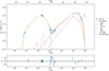 |
Fig. 10. Best-fit model for the broadband SED of OP 313 Flare 1 computed using the JeTSet ModelMinimizer module. The legend provides the color coding for the different components. |
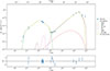 |
Fig. 11. Best-fit model for the broadband SED of OP 313 Flare 5, computed using the JeTSet ModelMinimizer module. The legend provides the color coding for the different components. |
Table 7 shows the best-fit parameters, along with the corresponding uncertainties, resulting from the MCMC fit.
Posterior parameters for the broadband SEDs of OP 313 in Flare 1 and Flare 5.
We computed the magnetic energy density over the electron energy density (uB/ue) ratio for the two flaring periods to assess the magnetization of the emitting region. Using the values reported in Table 7, we obtained uB/ue values equal to 0.031 and 0.013 for Flare 1 and Flare 5, respectively, with
 (16)
(16)
 (17)
(17)
where mec2 is the rest energy of the electron and n(γ) is the electron population described in Equation (11). These values indicate that the emission region is particle-dominated, with a relatively low magnetic energy density compared to the energy carried by relativistic electrons.
The two-flaring period SEDs exhibits the typical two-bump structure commonly associated with blazars, where the low-energy peak is attributed to synchrotron radiation and the HE peak arises from inverse Compton scattering. However, the relative contributions of different components vary between the two flaring periods, reflecting distinct physical conditions in the jet and its surroundings. The observed fluxes for both flaring periods at high energy are well explained by the model with SSC and EC emission mechanisms, as seen in Figures 10 and 11. In both cases, the EC dominates over the SSC emission, with a lower Compton dominance (CD) in the first one (CD ≈ 1).
As discussed in Sect. 3.4, the γ-ray flares are likely associated with new components merging from the VLBA core, which places the emission regions rather far from the central engine. This is also in agreement with the studies of Kramarenko et al. (2022) and Costamante et al. (2018) that places the γ-ray emission region outside the BLR, and with the detection of the source up to energies 250 GeV by LST-1 and MAGIC (Baxter et al. 2025). If the emission region was inside the BLR, the γ-rays of such high energies would be absorbed (e.g., Tavecchio & Mazin 2009).
Hence, for both flaring periods, we set RH to have the emission region outside the BLR and show the DT as the main source of seed photons. The change in the parameters between Flare 1 and 5, i.e., an increase of RH, and a consequent increase of R (due to the jet geometry), with a decrease of the magnetic field, are qualitatively consistent with an adiabatically expanding blob moving along the axis of a conical jet. This could be in agreement with the results presented in Section 3.4. This scenario, investigated in Tramacere et al. (2022), would also imply a very mild decrease in the total number of particles (if particle escape is very inefficient), and a magnetic field value dictated by the flux-freezing theorem B(R(t)) = B0(R0/R(t))mB (Begelman et al. 1984). However, this interpretation is not unique. The inferred distance traveled in time between flares suggests only mildly relativistic motion, which is inconsistent with the assumed bulk Lorentz factor. A purely adiabatic expansion would likely produce a more continuous high-flux state rather than temporally distinct flares, as we see in the light curve. As shown in Section 3.4, we found that before the 2024 flaring activity, new components arose from the jet and could collide with the first static shock. Hence, it is likely that an additional shock acceleration occurred during Flare 5, on top of the expansion. Hence, while our modeling suggests the adiabatic expansion as a plausible scenario, alternative combinations of parameters (e.g., lower B or higher Γ) and physical mechanisms, like turbulence and kink instabilities, may yield comparable fits. Further multiwavelength constraints would be required to break this degeneracy. In particular, the obtained magnetic fields and Doppler factors are consistent with internal shocks within the relativistic jets (e.g., Marscher & Gear 1985; Böttcher & Dermer 2010), but moderate changes of these parameters could also point to turbulence-driven particle acceleration (e.g., Marscher 2014; Chen et al. 2016) or magnetic reconnection and kink-instability scenarios (e.g., Giannios et al. 2009; Barniol Duran et al. 2017; Tchekhovskoy & Bromberg 2016).
Dar et al. (2025) proposes that a hadronic component contributed to the flaring emission of OP 313. Dar et al. (2025) suggests that, in the period in which we identify the Flare 2 and 3, the inclusion of the photo-meson process along with the leptonic emission component can successfully reproduce the SED, while the leptonic one cannot. However, the optical-gamma correlation we see suggests a rather leptonic origin (see Section 3.2.3). We also note that this is the period in which the very high energy (VHE) gamma-ray emission from OP 313, was detected, and the goodness of the leptonic fit will be further investigated in the upcoming paper by MAGIC and LST Collaborations (Baxter et al. 2025).
4. Summary
We have presented multiwavelength observations of the high redshift FSRQ OP 313 during 2008–2024, including radio-to-γ-ray data collected by LAT, Swift, ATLAS, CRTS, KAIT, Tuorla, ZTF, Metshäovi, VLBA, QUIVER, SMAPOL, and the F-GAMMA project. Strong variability has been observed from optical to γ rays, with an increasing flux starting from 2022. The optical, UV, X-ray, and γ-ray light curves are well correlated. A different behavior has been observed in radio, with the flux being high in 2008 and a new increasing trend in 2019, without a clear correlation with the other bands.
Focusing on the γ-ray observations, in particular those after 2021, we identified seven flaring periods and investigated the interplay between particle acceleration and radiative cooling in the source’s jet by means of hysteresis plots. We found no clear hysteresis pattern for the first, second, and fifth flaring periods. The SED of the fifth γ-ray flaring period shows a significant Compton dominance, suggesting that photon fields outside the jet are responsible for the IC scattering. This is in agreement with the results shown in Kramarenko et al. (2022) that identify the γ-ray emission region to be outside the BLR. Moreover, an overall correlation has been observed between optical and γ-ray bands without significant time lag, suggesting that the emission in these two bands has a common origin and is produced by leptonic processes.
The kinematics of the jet were investigated through the analysis of high-resolution radio images collected from the VLBA-BU-BLAZAR and MOJAVE projects. New components were found to arise in the jet starting from 2021, and we argued that some of them could be responsible for the flaring activity observed since 2022. To investigate this possibility, we calculated the epoch of ejection and the epoch at which the knots encountered a standing shock in the jet. As a result, we claim that the knots named “B11” could be responsible for the flaring activity observed in 2022–2023. We modeled the SEDs of the first and fifth flaring periods using a single-zone model that includes both SSC and EC components to test the scenario in which the γ-ray emitting region is located far from the central engine and the dusty torus acts as the dominant source of seed photons. This analysis shows that the DT component is more prominent in the fifth flaring period, in agreement with expectations. This highlights the crucial role of the DT’s photon field in accounting for the γ-ray emission of OP 313. This outcome is also consistent with the detection of the source at energies up to 250 GeV by the LST-1 and MAGIC telescopes, since photons of such high energy would be absorbed if emitted within the BLR (e.g., Tavecchio & Mazin 2009). Therefore, detailed modeling of the spectral energy distribution during flare 3, using the VHE γ-ray data (LST-1 and MAGIC Collaborations, in prep.), could further strengthen this conclusion. Further study of jet kinematics, including the most recent VLBA data (Jorstad et al., in prep.), will also be valuable in confirming the “far-from-the-black-hole” emission scenario outlined in this paper.
Acknowledgments
Author Contributions. C. Bartolini: project leadership, Fermi-LAT data analysis, Swift data analysis, VLBA data analysis, theoretical modeling, paper drafting and editing; E. Lindfors: optical data analysis, interpretation, and paper editing; D. Cerasole: Swift data analysis, optical and γ-ray correlation study, paper editing; A. Tramacere: theoretical modeling and paper drafting; A. Lähteenmäki and M. Tornikoski: Metsähovi data analysis. The rest of the authors have contributed in one or several of the following ways: data acquisition, processing, calibration, and/or reduction; cross-check of the data analysis; draft editing. C.B.: This paper and related research have been conducted during and with the support of the Italian national inter-university PhD program in Space Science and Technology. C.B.: Thanks to Beyoncè’s songs for giving her the necessary strength to write this paper during a difficult time. F.G.: acknowledges financial support from Junta de Castilla y León project SA101P24. J.J.: was supported by Academy of Finland projects 320085 and 345899 P.K.: was supported by Academy of Finland projects 346071 and 345899. The Fermi-LAT Collaboration acknowledges generous ongoing support from a number of agencies and institutes that have supported both the development and the operation of the LAT as well as scientific data analysis. These include the National Aeronautics and Space Administration and the Department of Energy in the United States, the Commissariat à l’Energie Atomique and the Centre National de la Recherche Scientifique/Institut National de Physique Nucléaire et de Physique des Particules in France, the Agenzia Spaziale Italiana and the Istituto Nazionale di Fisica Nucleare in Italy, the Ministry of Education, Culture, Sports, Science and Technology (MEXT), High Energy Accelerator Research Organization (KEK) and Japan Aerospace Exploration Agency (JAXA) in Japan, and the K. A. Wallenberg Foundation, the Swedish Research Council and the Swedish National Space Board in Sweden. Additional support for science analysis during the operations phase is gratefully acknowledged from the Istituto Nazionale di Astrofisica in Italy and the Centre National d’Études Spatiales in France. This work performed in part under DOE Contract DE-AC02-76SF00515. This research has made use of the NASA/IPAC Infrared Science Archive, which is funded by the National Aeronautics and Space Administration and operated by the California Institute of Technology. This publication makes use of data obtained at Metsähovi Radio Observatory, operated by Aalto University in Finland. This publication makes use of data based on observations with the 100 m telescope of the MPIfR (Max-Planck-Institut für Radioastronomie). I.M., I.N. and V.K. were funded by the International Max Planck Research School (IMPRS) for Astronomy and Astrophysics at the Universities of Bonn and Cologne. This research has made use of data from the MOJAVE database that is maintained by the MOJAVE team (Lister et al. 2018). This study makes use of VLBA data from the VLBA-BU Blazar Monitoring Program (BEAM-ME and VLBA-BU-BLAZAR; http://www.bu.edu/blazars/BEAM-ME.html), funded by NASA through the Fermi Guest Investigator Program. The VLBA is an instrument of the National Radio Astronomy Observatory. The National Radio Astronomy Observatory is a facility of the National Science Foundation operated by Associated Universities, Inc. This research has made use of data from the MOJAVE database that is maintained by the MOJAVE team (Lister et al. 2018). Partly based on observations with the 100-m telescope of the MPIfR (Max-Planck-Institut für Radioastronomie) at Effelsberg. Observations with the 100-m radio telescope at Effelsberg have received funding from the European Union’s Horizon 2020 research and innovation programme under grant agreement No 101004719 (ORP). The Submillimeter Array is a joint project between the Smithsonian Astrophysical Observatory and the Academia Sinica Institute of Astronomy and Astrophysics and is funded by the Smithsonian Institution and the Academia Sinica. Maunakea, the location of the SMA, is a culturally important site for the indigenous Hawaiian people; we are privileged to study the cosmos from its summit. This work has made use of data from the Joan Oró Telescope (TJO) of the Montsec Observatory (OdM), which is owned by the Catalan Government and operated by the Institute for Space Studies of Catalonia (IEEC). Based on observations obtained with the Samuel Oschin Telescope 48-inch and the 60-inch Telescope at the Palomar Observatory as part of the Zwicky Transient Facility project. ZTF is supported by the National Science Foundation under Grant No. AST-2034437 and a collaboration including Caltech, IPAC, the Weizmann Institute for Science, the Oskar Klein Center at Stockholm University, the University of Maryland, Deutsches Elektronen-Synchrotron and Humboldt University, the TANGO Consortium of Taiwan, the University of Wisconsin at Milwaukee, Trinity College Dublin, Lawrence Livermore National Laboratories, and IN2P3, France. Operations are conducted by COO, IPAC, and UW. The ZTF forced-photometry service was funded under the Heising-Simons Foundation grant #12540303 (PI: M.J. Graham). This work has made use of data from the Asteroid Terrestrialimpact Last Alert System (ATLAS) project. The Asteroid Terrestrial-impact Last Alert System (ATLAS) project is primarily funded to search for near earth asteroids through NASA grants NN12AR55G, 80NSSC18K0284, and 80NSSC18K1575; byproducts of the NEO smarch include images and catalogs from the survey area. This work was partially funded by Kepler/K2 grant J1944/80NSSC19K0112 and HST GO-15889, and STFC grants ST/T000198/1 and ST/S006109/1. The ATLAS science products have been made possible through the contributions of the University of Hawaii Institute for Astronomy, the Queen’s University Belfast, the Space Telescope Science Institute, the South African Astronomical Observatory, and The Millennium Institute of Astrophysics (MAS), Chile.
References
- Abdollahi, S., Acero, F., Ackermann, M., et al. 2020, ApJS, 247, 33 [Google Scholar]
- Abdollahi, S., Acero, F., Baldini, L., et al. 2022, ApJS, 260, 53 [NASA ADS] [CrossRef] [Google Scholar]
- Abe, K., Abe, S., Abhir, J., et al. 2025, A&A, 697, A172 [NASA ADS] [CrossRef] [EDP Sciences] [Google Scholar]
- Acharyya, A., & Sadun, A. C. 2023, Galaxies, 11, 81 [Google Scholar]
- Ackermann, M., Anantua, R., Asano, K., et al. 2016, ApJ, 824, L20 [NASA ADS] [CrossRef] [Google Scholar]
- Aharonian, F. A. 2000, New Astron., 5, 377 [NASA ADS] [CrossRef] [Google Scholar]
- Aharonian, F., Akhperjanian, A. G., Bazer-Bachi, A. R., et al. 2007, ApJ, 664, L71 [NASA ADS] [CrossRef] [Google Scholar]
- Alexander, T. 1997, Astronomical Time Series (Dordrecht: Kluwer), 163 [Google Scholar]
- Angel, J. R. P., & Stockman, H. S. 1980, ARA&A, 18, 321 [NASA ADS] [CrossRef] [Google Scholar]
- Angelakis, E., Fuhrmann, L., Myserlis, I., et al. 2019, A&A, 626, A60 [NASA ADS] [CrossRef] [EDP Sciences] [Google Scholar]
- Arnaud, K. A. 1996, ASP Conf. Ser., 101, 17 [Google Scholar]
- Atwood, W. B., Abdo, A. A., Ackermann, M., et al. 2009, ApJ, 697, 1071 [CrossRef] [Google Scholar]
- Atwood, W., Albert, A., Baldini, L., et al. 2013, ArXiv e-prints [arXiv:1303.3514] [Google Scholar]
- Barniol Duran, R., Tchekhovskoy, A., & Giannios, D. 2017, MNRAS, 469, 4957 [NASA ADS] [CrossRef] [Google Scholar]
- Barthelmy, S. D., Barbier, L. M., Cummings, J. R., et al. 2005, Space Sci. Rev., 120, 143 [Google Scholar]
- Bartolini, C. 2024, ATel, 16497, 1 [Google Scholar]
- Bartolini, C., Giacchino, F., Elenterio, D., & Gisonna, M. S. 2023, ATel, 16356, 1 [Google Scholar]
- Baxter, J., Takeishi, R., Arbet-Engels, A., et al. 2025, in Proceedings of 39th International Cosmic Ray Conference — PoS(ICRC2025), 501, 569 [Google Scholar]
- Begelman, M. C., Blandford, R. D., & Rees, M. J. 1984, Rev. Mod. Phys., 56, 255 [Google Scholar]
- Bellm, E. C., Kulkarni, S. R., Graham, M. J., et al. 2018, PASP, 131, 018002 [Google Scholar]
- Blandford, R., Meier, D., & Readhead, A. 2019, ARA&A, 57, 467 [NASA ADS] [CrossRef] [Google Scholar]
- Böttcher, M., & Dermer, C. D. 2010, ApJ, 711, 445 [CrossRef] [Google Scholar]
- Böttcher, M., Reimer, A., Sweeney, K., & Prakash, A. 2013, ApJ, 768, 54 [Google Scholar]
- Britzen, S., Qian, S. J., Steffen, W., et al. 2017, A&A, 602, A29 [NASA ADS] [CrossRef] [EDP Sciences] [Google Scholar]
- Bruel, P., Burnett, T. H., Digel, S. W., et al. 2018, ArXiv e-prints [arXiv:1810.11394] [Google Scholar]
- Burrows, D. N., Hill, J. E., Nousek, J. A., et al. 2005, Space Sci. Rev., 120, 165 [Google Scholar]
- Buson, S. 2014, ATel, 6068, 1 [Google Scholar]
- Casadio, C., Gómez, J. L., Jorstad, S. G., et al. 2015, ApJ, 813, 51 [Google Scholar]
- Chen, X., Pohl, M., Böttcher, M., & Gao, S. 2016, MNRAS, 458, 3260 [Google Scholar]
- Cleary, K., Lawrence, C. R., Marshall, J. A., Hao, L., & Meier, D. 2007, ApJ, 660, 117 [CrossRef] [Google Scholar]
- Connolly, S. D. 2016, Astrophysics Source Code Library [record ascl:1602.012] [Google Scholar]
- Cortina, J. 2023, ATel, 16381, 1 [NASA ADS] [Google Scholar]
- Costamante, L., Cutini, S., Tosti, G., Antolini, E., & Tramacere, A. 2018, MNRAS, 477, 4749 [Google Scholar]
- Dar, A. A., Shah, Z., Sahayanathan, S., et al. 2025, ApJ, submitted [arXiv:2503.01583] [Google Scholar]
- Dembinski, H., Ongmongkolkul, P., & Deil, C. 2020, https://github.com/scikit-hep/iminuit [Google Scholar]
- Dermer, C. D., & Schlickeiser, R. 1993, ApJ, 416, 458 [Google Scholar]
- Dermer, C. D., Finke, J. D., Krug, H., & Böttcher, M. 2009, ApJ, 692, 32 [NASA ADS] [CrossRef] [Google Scholar]
- Donea, A.-C., & Protheroe, R. J. 2003, Astropart. Phys., 18, 377 [Google Scholar]
- Drake, A. J., Djorgovski, S. G., Mahabal, A., et al. 2009, ApJ, 696, 870 [Google Scholar]
- Edelson, R. A. 1988, ApJ, 333, 646 [NASA ADS] [CrossRef] [Google Scholar]
- Emmanoulopoulos, D., McHardy, I. M., & Papadakis, I. E. 2013, MNRAS, 433, 907 [NASA ADS] [CrossRef] [Google Scholar]
- Filippenko, A. V., Li, W. D., Treffers, R. R., & Modjaz, M. 2001, ASP Conf. Ser., 246, 121 [NASA ADS] [Google Scholar]
- Finke, J. D. 2013, ApJ, 763, 134 [NASA ADS] [CrossRef] [Google Scholar]
- Foreman-Mackey, D., Hogg, D. W., Lang, D., & Goodman, J. 2013, PASP, 125, 306 [Google Scholar]
- Franceschini, A., Rodighiero, G., & Vaccari, M. 2008, A&A, 487, 837 [NASA ADS] [CrossRef] [EDP Sciences] [Google Scholar]
- Fuhrmann, L., Angelakis, E., Zensus, J. A., et al. 2016, A&A, 596, A45 [NASA ADS] [CrossRef] [EDP Sciences] [Google Scholar]
- Gabuzda, D. C., Kollgaard, R. I., Roberts, D. H., & Wardle, J. F. C. 1993, ApJ, 410, 39 [NASA ADS] [CrossRef] [Google Scholar]
- Garrappa, S. 2022, ATel, 15483, 1 [Google Scholar]
- Garrappa, S., Buson, S., Franckowiak, A., et al. 2019, ApJ, 880, 103 [NASA ADS] [CrossRef] [Google Scholar]
- Gehrels, N., Chincarini, G., Giommi, P., et al. 2004, ApJ, 611, 1005 [Google Scholar]
- Ghisellini, G., & Tavecchio, F. 2015, MNRAS, 448, 1060 [NASA ADS] [CrossRef] [Google Scholar]
- Giannios, D., Uzdensky, D. A., & Begelman, M. C. 2009, MNRAS, 395, L29 [NASA ADS] [CrossRef] [Google Scholar]
- Gurwell, M. A., Peck, A. B., Hostler, S. R., Darrah, M. R., & Katz, C. A. 2007, ASP Conf. Ser., 375, 234 [NASA ADS] [Google Scholar]
- Ho, P. T. P., Moran, J. M., & Lo, K. Y. 2004, ApJ, 616, L1 [Google Scholar]
- Hovatta, T., Valtaoja, E., Tornikoski, M., & Lähteenmäki, A. 2009, A&A, 494, 527 [CrossRef] [EDP Sciences] [Google Scholar]
- Hovatta, T., Pavlidou, V., King, O. G., et al. 2014, MNRAS, 439, 690 [NASA ADS] [CrossRef] [Google Scholar]
- IceCube Collaboration (Aartsen, M. G., et al.) 2018, Science, 361, eaat1378 [NASA ADS] [Google Scholar]
- IceCube Collaboration (Abbasi, R., et al.) 2022, Science, 378, 538 [CrossRef] [PubMed] [Google Scholar]
- Inoue, S., & Takahara, F. 1996, ApJ, 463, 555 [Google Scholar]
- Janiak, M., Sikora, M., & Moderski, R. 2015, MNRAS, 449, 431 [CrossRef] [Google Scholar]
- Jankov, I., Kovačević, A. B., Ilić, D., Sánchez-Sáez, P., & Nikutta, R. 2022, https://doi.org/10.5281/zenodo.7253034 [Google Scholar]
- Jannuzi, B. T., Smith, P. S., & Elston, R. 1993, ApJS, 85, 265 [Google Scholar]
- Jorstad, S. G., Marscher, A. P., Lister, M. L., et al. 2005, ApJ, 130, 1418 [Google Scholar]
- Jorstad, S. G., Marscher, A. P., Morozova, D. A., et al. 2017, ApJ, 846, 98 [Google Scholar]
- Kankkunen, S., Tornikoski, M., Hovatta, T., & Lähteenmäki, A. 2025, A&A, 693, A318 [NASA ADS] [CrossRef] [EDP Sciences] [Google Scholar]
- Kaspi, S., Brandt, W. N., Maoz, D., et al. 2007, ApJ, 659, 997 [NASA ADS] [CrossRef] [Google Scholar]
- Kelner, S. R., & Aharonian, F. A. 2008, Phys. Rev. D, 78, 034013 [Google Scholar]
- Kirk, J. G., Rieger, F. M., & Mastichiadis, A. 1998, A&A, 333, 452 [NASA ADS] [Google Scholar]
- Kouch, P. M., Lindfors, E., Hovatta, T., et al. 2024, A&A, 690, A111 [NASA ADS] [CrossRef] [EDP Sciences] [Google Scholar]
- Kramarenko, I. G., Pushkarev, A. B., Kovalev, Y. Y., et al. 2022, MNRAS, 510, 469 [Google Scholar]
- Kraus, A., Krichbaum, T. P., Wegner, R., et al. 2003, A&A, 401, 161 [NASA ADS] [CrossRef] [EDP Sciences] [Google Scholar]
- Liodakis, I., Hovatta, T., Huppenkothen, D., et al. 2018, ApJ, 866, 137 [Google Scholar]
- Liodakis, I., Romani, R. W., Filippenko, A. V., Kocevski, D., & Zheng, W. 2019, ApJ, 880, 32 [NASA ADS] [CrossRef] [Google Scholar]
- Liodakis, I., Hovatta, T., Aller, M. F., et al. 2021, A&A, 654, A169 [NASA ADS] [CrossRef] [EDP Sciences] [Google Scholar]
- Lister, M. L., Aller, H. D., Aller, M. F., et al. 2009, AJ, 137, 3718 [Google Scholar]
- Lister, M. L., Aller, M. F., Aller, H. D., et al. 2018, ApJS, 234, 12 [CrossRef] [Google Scholar]
- Lister, M. L., Homan, D. C., Hovatta, T., et al. 2019, ApJ, 874, 43 [NASA ADS] [CrossRef] [Google Scholar]
- Lister, M. L., Homan, D. C., Kellermann, K. I., et al. 2021, ApJ, 923, 30 [NASA ADS] [CrossRef] [Google Scholar]
- Lott, B., Escande, L., Larsson, S., & Ballet, J. 2012, A&A, 544, A6 [NASA ADS] [CrossRef] [EDP Sciences] [Google Scholar]
- Mangal, H. 2021, ATel, 14404, 1 [Google Scholar]
- Mannheim, K., & Biermann, P. L. 1992, A&A, 253, L21 [NASA ADS] [Google Scholar]
- Marscher, A. P. 2014, ApJ, 780, 87 [Google Scholar]
- Marscher, A. P., & Gear, W. K. 1985, ApJ, 298, 114 [Google Scholar]
- Mohana A, K., Gupta, A. C., Marscher, A. P., et al. 2024, MNRAS, 527, 6970 [Google Scholar]
- Mücke, A., & Protheroe, R. J. 2001, Astropart. Phys., 15, 121 [Google Scholar]
- Mücke, A., Protheroe, R. J., Engel, R., Rachen, J. P., & Stanev, T. 2003, Astropart. Phys., 18, 593 [Google Scholar]
- Myserlis, I., Angelakis, E., Kraus, A., et al. 2018, A&A, 609, A68 [NASA ADS] [CrossRef] [EDP Sciences] [Google Scholar]
- Nalewajko, K., & Gupta, M. 2017, A&A, 606, A44 [NASA ADS] [CrossRef] [EDP Sciences] [Google Scholar]
- Nilsson, K., Lindfors, E., Takalo, L. O., et al. 2018, A&A, 620, A185 [NASA ADS] [CrossRef] [EDP Sciences] [Google Scholar]
- Potter, W. J., & Cotter, G. 2013, MNRAS, 431, 1840 [Google Scholar]
- Rodrigues, X., Garrappa, S., Gao, S., et al. 2021, ApJ, 912, 54 [NASA ADS] [CrossRef] [Google Scholar]
- Roming, P. W. A., Kennedy, T. E., Mason, K. O., et al. 2005, Space Sci. Rev., 120, 95 [Google Scholar]
- Sambruna, R. M., Maraschi, L., & Urry, C. M. 1996, ApJ, 463, 444 [Google Scholar]
- Scargle, J. D., Norris, J. P., Jackson, B., & Chiang, J. 2013, ApJ, 764, 167 [Google Scholar]
- Schlafly, E. F., & Finkbeiner, D. P. 2011, ApJ, 737, 103 [Google Scholar]
- Schneider, D. P., Richards, G. T., Hall, P. B., et al. 2010, ApJ, 139, 2360 [Google Scholar]
- Seabold, S., & Perktold, J. 2010, Statsmodels: Econometric and Modeling with Python, 57 [Google Scholar]
- Shepherd, M. C. 1997, ASP Conf. Ser., 125, 77 [Google Scholar]
- Sikora, M., Begelman, M., & Rees, M. 1994, ApJ, 421, 153 [Google Scholar]
- Smith, P. S., Balonek, T. J., Heckert, P. A., & Elston, R. 1986, ApJ, 305, 484 [Google Scholar]
- Stickel, M., Padovani, P., & Urry, C. M. 1991, ApJ, 374, 431 [NASA ADS] [CrossRef] [Google Scholar]
- Tarnopolski, M., Żywucka, N., Marchenko, V., & Pascual-Granado, J. 2020, ApJS, 250, 1 [NASA ADS] [CrossRef] [Google Scholar]
- Tashiro, M., & Makishima, K. 1995, PASJ, 47, 131 [Google Scholar]
- Tavecchio, F., & Mazin, D. 2009, MNRAS, 392, L40 [Google Scholar]
- Tchekhovskoy, A., & Bromberg, O. 2016, MNRAS, 461, L46 [NASA ADS] [CrossRef] [Google Scholar]
- Teräsranta, H., Tornikoski, M., Mujunen, A., et al. 1998, A&AS, 132, 305 [NASA ADS] [CrossRef] [EDP Sciences] [Google Scholar]
- Timmer, J., & König, M. 1995, A&A, 300, 707 [Google Scholar]
- Tramacere, A. 2020, Astrophysics Source Code Library [record ascl:2009.001] [Google Scholar]
- Tramacere, A., Giommi, P., Perri, M., Verrecchia, F., & Tosti, G. 2009, A&A, 501, 879 [NASA ADS] [CrossRef] [EDP Sciences] [Google Scholar]
- Tramacere, A., Massaro, E., & Taylor, A. M. 2011, ApJ, 739, 66 [Google Scholar]
- Tramacere, A., Sliusar, V., Walter, R., Jurysek, J., & Balbo, M. 2022, A&A, 658, A173 [NASA ADS] [CrossRef] [EDP Sciences] [Google Scholar]
- Watson, D., Smith, N., Hanlon, L., et al. 2000, A&A, 364, 43 [NASA ADS] [Google Scholar]
- Weaver, Z. R., Jorstad, S. G., Marscher, A. P., et al. 2022, ApJS, 260, 12 [NASA ADS] [CrossRef] [Google Scholar]
- Wills, B. J., & Wills, D. 1979, ApJS, 41, 689 [NASA ADS] [CrossRef] [Google Scholar]
- Wood, M., Caputo, R., Charles, E., et al. 2018, Proc. Sci., 301, 824 [Google Scholar]
- Xu, M. H., Anderson, J. M., Heinkelmann, R., et al. 2019, ApJS, 242, 5 [Google Scholar]
We employed the LogParabola model as defined in https://fermi.gsfc.nasa.gov/ssc/data/analysis/scitools/source_models.html
Appendix A: Hysteresis patterns in 2-day long time bins
In Figure A.1a, A.1b, and A.1c, we show how the hysteresis patterns of the first, the second, and the fifth flaring periods are if we consider the average photon index in 2-day-long time bins. The hysteresis pattern’s hints we find are anti-clockwise for the first and the fifth flaring periods, and clockwise for the second flaring period. This feature shows why we can not establish that our patterns are truly clockwise or anti-clockwise due to the large photon index error bars, and how they and the average flux change considering different time bins.
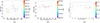 |
Fig. A.1. a) First flaring period hysteresis pattern from 2 July 2022 to 15 July 2022, considering 2-day-long time bins. The dashed gray line is drawn to help seek the correct order of the points. b) Fifth flaring period hysteresis pattern from 30 January 2024 to 8 February 2024, considering 2-day-long time bins. c) Second flaring period hysteresis pattern from 20 November 2023 to 29 November 2023, considering 2-day-long time bins. |
Appendix B: MOJAVE and VLBA-BU-BLAZAR tables
Table B.1 describes the fits as follows: 1- ID of the component; 2– mean flux density and error in mJy; 3- mean projected distance from the core feature in mas; 4- mean position angle of feature with respect to the core component; 5- angular proper motion in milliarcseconds per year; 6- proper motion in units of the speed of light; 7- acceleration in milliarcsecond per square year; 8- date of reference (middle) epoch used for fit. Table B.2 describes the fits as follows: 1- ID of the component; 2– mean flux density and error in mJy; 3- mean projected distance from the core feature in mas; 4- mean position angle of feature with respect to the core component; 5- angular proper motion in milliarcseconds per year; 6- proper motion in units of the speed of light; 7- parallel acceleration the jet in milliarcsecond per square year; 8- perpendicular acceleration the jet in milliarcsecond per square year.
Jet structure and kinematic parameters of the MOJAVE dataset.
Jet structure and kinematic parameters of the VLBA-BU-BLAZAR dataset.
Appendix C: SED modeling table and plots
Figure C.1a shows the broadband SED of OP 313’s Flare 1 and C.1b shows the broadband SED of OP 313’s Flare 5 using JeTSet McmcSampler.
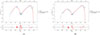 |
Fig. C.1. (a) Model-fit broadband SED of OP 313’s Flare 1 and (b) model-fit broadband SED of OP 313’s Flare 5 using JeTSet McmcSampler. The legends provide the color coding for the MCMC information. |
All Tables
Instruments whose datasets have been included for the long-term MWL analysis of OP 313.
Doppler factor (δvar), Lorentz factor (Γ), and viewing angle (Θ0) of the new components detected from 2019 in VLBA-BU-BLAZAR visibilities.
Lorentz factor (Γvar) and viewing angle (Θ0) of the new components arisen from 2019 in the visibilities of the VLBA-BU-BLAZAR project.
Epoch of ejection T0 and epoch in which the knot encounters the static shock T1 for the new knots found in the VLBA-BU-BLAZAR data.
Epoch of ejection T0 and epoch in which the knot encounters the static shock T1 for component 24.
All Figures
|
Fig. 1. Top: 15-year Fermi-LAT light curve of OP 313, divided into quiescent (blue) and flaring (yellow) states. The green line shows the time-weighted average flux of 4.93 × 10⁻⁸ photons/cm2s computed between 9 December 2014 and 9 August 2018. Bottom: Fermi-LAT photon index over the same 15-year period. The green line shows the average photon index computed between 9 December 2014 and 9 August 2018 (Γ = 2.39), with the green band indicating its corresponding 1σ uncertainty. The red vertical bands highlight the period in which LST-1 detected OP 313. |
| In the text | |
|
Fig. 2. Multiwavelength light curve of OP 313. The red vertical band indicates the period when LST-1 detected OP 313. a: Fermi-LAT light curve at E > 100 MeV. b: Swift-XRT X-ray light curve from 0.3 keV to 10 keV. c: Swift-UVOT light curve in the optical/UV bands. d: Optical light curve from several facilities and filters: CRTS V-filter (cV), KAIT R-filter (kR), Tuorla R-filter (tR), ATLAS o (Ao) and c-filters (Ac), and Palomar ZTF g, r, and i-filters (zG, zR, and zI). The label zGzR refers to ZTF observations using both g and r filters. e: Radio Single Dish FERMI-GST AGN Multi-frequency Monitoring Alliance (F-GAMMA) light curves above 15 GHz, Submillimeter Array (SMA) data at 225, 273 and 350 GHz, including SMAPOL data at 225 GHz light curves, Metsähovi at 37 GHz and VLBA-BU-BLAZAR at 43 GHz light curves. f: Radio Single Dish F-GAMMA light curves below 15 GHz and MOJAVE VLBA light curve. |
| In the text | |
|
Fig. 3. Fermi-LAT (top) and optical (bottom) light curves from 1 January 2022 to 9 March 2024. The dashed black lines indicate the brightest γ-ray flaring periods. The fourth and sixth flaring periods are not between the brightest but are located in time between the ATels Bartolini et al. (2023) and Bartolini (2024). The red vertical bands indicate the period when LST-1 detected OP 313. |
| In the text | |
|
Fig. 4. (a) Hysteresis pattern of the first flaring period (2 July 2022 – 15 July 2022). The dashed gray line is included to guide the eye in identifying the temporal sequence of the points. (b) Hysteresis pattern of the fifth flaring period (30 January 2024 – 8 February 2024). (c) Hysteresis pattern of the second flaring period (20 November 2023 – 29 November 2023). |
| In the text | |
|
Fig. 5. SED of the first (2022), in orange, the fifth flaring periods (January 2024), in blue, and a quiescent period that goes from March 2016 to January 2018, in purple. The X-ray, UV, optical, and radio SED points correspond to the average flux values within each period at their respective frequencies. No Swift-XRT and UVOT data were available during the quiescent period. |
| In the text | |
|
Fig. 6. (a) zDCF analysis on the short-term period of OP 313 optical and γ-ray light curves; and (b) distribution of the reconstructed zDCF at zero time-lag for 104 simulated uncorrelated γ-ray and optical light curves. The red line marks the reconstructed zDCF value with the observed OP 313 light curves in Figure 3. |
| In the text | |
|
Fig. 7. Angular separation from the core versus time for Gaussian jet features of the MOJAVE data. Colored symbols indicate robust features for which kinematic fits were obtained. The 1σ positional errors on the individual points typically range from 10% of the FWHM restoring beam dimension for isolated compact features to 20%, represented as a black cross in the plot, of the FWHM for weak features (see e.g., Lister et al. 2009, 2019, 2021). |
| In the text | |
|
Fig. 8. Angular separation from the core versus time for Gaussian jet features of the VLBA-BU-BLAZAR (VLBA-BU-BLAZAR) data. Colored symbols indicate robust features for which kinematic fits were obtained. The 2 dashed lines in yellow and purple represent the static shocks’ mean distance from the core. |
| In the text | |
|
Fig. 9. Comparison between the Fermi-LAT data (in blue) with their Bayesian blocks (in black) and the total flux density of MOJAVE data at 15 GHz (in red). The dashed blue lines represent the time of ejections for different knots, found in the VLBA-BU-BLAZAR visibilities, and the blue lines are the corresponding errors, while the orange dashed lines represent the epochs when the knots encounter the standing shock “A1” with the corresponding errors. In green, the epoch in which “B12” was found. |
| In the text | |
|
Fig. 10. Best-fit model for the broadband SED of OP 313 Flare 1 computed using the JeTSet ModelMinimizer module. The legend provides the color coding for the different components. |
| In the text | |
|
Fig. 11. Best-fit model for the broadband SED of OP 313 Flare 5, computed using the JeTSet ModelMinimizer module. The legend provides the color coding for the different components. |
| In the text | |
|
Fig. A.1. a) First flaring period hysteresis pattern from 2 July 2022 to 15 July 2022, considering 2-day-long time bins. The dashed gray line is drawn to help seek the correct order of the points. b) Fifth flaring period hysteresis pattern from 30 January 2024 to 8 February 2024, considering 2-day-long time bins. c) Second flaring period hysteresis pattern from 20 November 2023 to 29 November 2023, considering 2-day-long time bins. |
| In the text | |
|
Fig. C.1. (a) Model-fit broadband SED of OP 313’s Flare 1 and (b) model-fit broadband SED of OP 313’s Flare 5 using JeTSet McmcSampler. The legends provide the color coding for the MCMC information. |
| In the text | |
Current usage metrics show cumulative count of Article Views (full-text article views including HTML views, PDF and ePub downloads, according to the available data) and Abstracts Views on Vision4Press platform.
Data correspond to usage on the plateform after 2015. The current usage metrics is available 48-96 hours after online publication and is updated daily on week days.
Initial download of the metrics may take a while.