| Issue |
A&A
Volume 707, March 2026
|
|
|---|---|---|
| Article Number | A213 | |
| Number of page(s) | 19 | |
| Section | Extragalactic astronomy | |
| DOI | https://doi.org/10.1051/0004-6361/202556654 | |
| Published online | 09 March 2026 | |
Multiwavelength properties of changing-state active galactic nuclei
I. The evolution of soft excess and X-ray continuum
1
Instituto de Estudios Astrofísicos, Facultad de Ingeniería y Ciencias, Universidad Diego Portales, Av. Ejército Libertador 441, Santiago, Chile
2
Department of Physics, SRM University-AP, Amaravati, 522240, Andhra Pradesh, India
3
Department of Astronomy, University of Geneva, ch. d’Ecogia 16, 1290 Versoix, Switzerland
4
Kavli Institute for Astronomy and Astrophysics, Peking University, Beijing 100871, PR China
5
INAF-Osservatorio Astronomico di Roma, via di Frascati 33, I-00078 Monte Porzio Catone, Italy
6
School of Physics and Astronomy, Tel Aviv University, Tel Aviv 69978, Israel
7
Max-Planck-Institut für extraterrestrische Physik, Gießenbachstraße 1, 85748 Garching, Germany
8
Excellence Cluster ORIGINS, Boltzmannsstraße 2, 85748 Garching, Germany
9
Instituto de Alta Investigación, Universidad de Tarapacá, Casilla 7D Arica, Chile
10
Centre for Extragalactic Astronomy, Department of Physics, Durham University, South Road, Durham DH1 3LE, UK
11
Eureka Scientific, 2452 Delmer Street, Suite 100, Oakland, CA 94602-3017, USA
12
Space Science Institute, 4750 Walnut Street, Suite 205, Boulder, CO 80301, USA
13
STAR Institute, Liège Université, Quartier Agora – Allée du six Août, 19c, B-4000 Liège, Belgium
14
Sterrenkundig Observatorium, Universiteit Gent, Krijgslaan 281 S9, B-9000 Gent, Belgium
15
Institute of Astronomy, National Tsing Hua University, Hsinchu 300044, Taiwan
16
Department of Astronomy, Faculty of Mathematics, University of Belgrade, Studentski trg 16, 11000 Belgrade, Serbia
17
Hamburger Sternwarte, Universitat Hamburg, Gojenbergsweg 112, D-21029 Hamburg, Germany
18
Humboldt Research Fellow, Max-Planck-Institut für Radioastronomie, Auf dem Hügel 69, Bonn D-53121, Germany
★ Corresponding author: This email address is being protected from spambots. You need JavaScript enabled to view it.
Received:
29
July
2025
Accepted:
8
January
2026
Abstract
Changing-state active galactic nuclei (CSAGNs) exhibit rapid variability; their mass accretion rates can change by several orders of magnitude in a few years. This provides us with a unique opportunity to study the evolution of the inner accretion flow almost in real time. Here we used over 1000 observations to study the broadband X-ray spectra of a sample of five CSAGNs, spanning three orders of magnitude in Eddington ratio (λEdd), using phenomenological models to trace the evolution of key spectral components. We derive several fundamental parameters, such as the photon index, soft excess strength, reflection strength, and luminosities of the soft excess and primary continuum. We find that the soft excess and primary continuum emissions show a very strong positive correlation (p ≪ 10−10), suggesting a common physical origin. The soft excess strength does not show any dependence on the reflection parameter, suggesting that in these objects the soft excess is not dominated by a blurred ionized reflection process. On the other hand, the strength of the soft excess is found to be strongly positively correlated with the Eddington ratio (p ≪ 10−10), and we find that the soft excess vanishes below log λEdd ∼ −2.5. Moreover, we find a clear V-shaped relation for Γ − λEdd, with a break at log λEdd = −2.47 ± 0.09. Our findings indicate a change in the geometry of the inner accretion flow at low Eddington ratios, and that the soft excess is primarily produced via warm Comptonization.
Key words: accretion, accretion disks / galaxies: active / galaxies: nuclei / quasars: supermassive black holes / X-rays: galaxies
© The Authors 2026
 Open Access article, published by EDP Sciences, under the terms of the Creative Commons Attribution License (https://creativecommons.org/licenses/by/4.0), which permits unrestricted use, distribution, and reproduction in any medium, provided the original work is properly cited.
This article is published in open access under the Subscribe to Open model. This email address is being protected from spambots. You need JavaScript enabled to view it. to support open access publication.
1. Introduction
Active galactic nuclei (AGNs) are powered by accreting supermassive black holes (SMBHs) located at galaxy centers (Rees 1988). Matter from the surrounding medium accretes onto the black hole through a geometrically thin, optically thick accretion disk. As the material spirals inward, its gravitational potential energy is efficiently converted into radiation, which is emitted across the entire electromagnetic spectrum. The inner accretion flow consists of a geometrically thin, optically thick disk and a compact X-ray corona. Such a disk emits mainly in UV/optical, thus producing the characteristic big blue bump in the spectral energy distribution (SED; Shakura & Sunyaev 1973; Malkan & Sargent 1982; Koratkar et al. 1995), while inverse Compton scattering of the UV photons by hot electrons in the corona produces a power-law X-ray continuum (Sunyaev & Titarchuk 1980; Haardt & Maraschi 1991). Additional excess emission above the power-law continuum is commonly observed below ∼1 − 2 keV, and is known as the soft excess (SE; Singh et al. 1985; Arnaud et al. 1985). The origin of this SE remains the subject of debate. Two primary scenarios have been proposed to explain the SE: (i) ionized reflection from the inner accretion disk (Crummy et al. 2006; Walton et al. 2013; Dauser et al. 2014) and (ii) thermal Comptonization in a warm corona (Done et al. 2012; Petrucci et al. 2013). In the ionized reflection model, SE arises from blurred ionized reflection, where fluorescent lines from reprocessed X-ray emission are smeared due to the strong gravitational field near the SMBH (e.g., Ross & Fabian 2005; García & Kallman 2010; Dauser et al. 2016; Ding et al. 2024). In contrast, the warm corona model attributes the SE to thermal Comptonization of seed photons from the AD in an optically thick, warm plasma (e.g., Magdziarz et al. 1998; Petrucci et al. 2018), which is distinct from the hot corona (kTh ∼ 50 − 100 keV; τh ≲ 1) responsible for the primary X-ray power-law emission. The warm corona is typically characterized by an electron temperature of kTw ∼ 0.1 − 0.2 keV and an optical depth of τw ∼ 10 − 20 (Petrucci et al. 2018). A hybrid origin involving both components is also proposed (García et al. 2019; Laha et al. 2022; Xiang et al. 2022; Chen et al. 2025).
Due to the high mass of the SMBHs (MBH ∼ 106 − 109 M⊙), the timescales expected for significant optical/UV variations in AGNs are expected to be ∼104 − 107 yr (e.g., Frank et al. 2002; Netzer 2013). Thus, major changes in accretion disk (AD) emission are in principle not expected to be observable on timescales of a few years. This limitation has been overcome by studying large samples of AGNs, which includes objects with very different accretion rates. This can offer some insights into the inner accretion flow dynamics across a wide range of accretion rates (e.g., Krolik 1999; Netzer 2013). A complementary approach involves studying black hole X-ray binaries (BHXBs), which can transition between different accretion states on timescales of months, allowing a detailed investigation of accretion physics (e.g., Remillard & McClintock 2006; Done et al. 2007). Despite the large difference in mass, AGNs might have similar accretion mechanisms to BHXBs (e.g., Merloni et al. 2003; McHardy et al. 2006), as suggested by their comparable spectral and timing properties (e.g., Sobolewska et al. 2011). However, some observational differences remain. For example, AGNs exhibit a soft X-ray excess (SE) below ∼1 − 2 keV not seen in BHXBs (Gierliński & Done 2004; Done et al. 2012; Ricci et al. 2017), for which the soft X-ray emission is often dominated by the accretion disk (e.g., Remillard & McClintock 2006). Additionally, AGNs display a dichotomy in radio loudness: Some sources launch powerful relativistic jets and others remain radio quiet, even at similar accretion rates (e.g., Sikora et al. 2007, see also Svoboda et al. 2017), while BHXBs show tighter correlations between jet activity and accretion state (Merloni et al. 2003; Fender & Belloni 2004).
Changing-state AGNs (CSAGNs) provide a unique opportunity to probe AGN accretion physics as their accretion rates can evolve by ∼1 − 2 orders of magnitude within weeks to years (e.g., MacLeod et al. 2016; Ruan et al. 2019; Trakhtenbrot et al. 2019; Temple et al. 2023; Ricci et al. 2021; Ricci & Trakhtenbrot 2023). In UV/optical wavebands, CSAGNs switch between type 1 states, with broad emission lines (BELs), and type 2 states, without broad emission lines, on timescales ranging from a few months to a few years (Stern et al. 2018; Noda & Done 2018). These transitions are primarily attributed to significant changes in the accretion rate (Sheng et al. 2017; Noda & Done 2018; Ricci & Trakhtenbrot 2023; Jana et al. 2025).
Accretion rate changes in CSAGNs are attributed to disk instabilities (Noda & Done 2018) or external perturbation, such as tidal disruptions (Merloni et al. 2015; Ricci et al. 2020). Noda & Done (2018) suggested that the SE ionizes the BLR, leading to BELs in type 1 states; however, in type 2 states, as SE intensity diminishes, BELs disappear. In Mrk 1018, the CS transition was accompanied by a decrease in the Eddington ratio (λEdd = Lbol/LEdd) from ∼0.08 to ∼0.006, while the primary X-ray continuum (PC) and SE flux decreased by factors of ∼7 and ∼60, respectively. SE evolution has been observed in other CSAGNs (e.g., Laha et al. 2022; Tripathi & Dewangan 2022; Layek et al. 2024), resembling soft to hard state transitions in BHXBs around λEdd ∼ 0.01 − 0.02 (e.g., Maccarone 2003; Done et al. 2007; Yang et al. 2015). A systematic study of optically identified CLAGNs using Swift/BAT light curves by Temple et al. (2023) showed significant 14 − 195 keV flux changes in most CLAGNs during optical transitions, suggesting these events are largely driven by accretion state changes. Using long-term optical and X-ray quasi-simultaneous observations, Jana et al. (2025) confirmed this picture, finding that transitions typically occur around  , consistent with other studies (e.g., Ruan et al. 2019; Ai et al. 2020),
The inner accretion geometry is expected to change at a few percent of the Eddington ratio (e.g., Esin et al. 1997; Yuan & Narayan 2014). This change is thought to be imprinted on the observed V-shaped photon index (Γ)–λEdd relation (e.g., Shemmer et al. 2006; Emmanoulopoulos et al. 2012; Trakhtenbrot et al. 2017; She et al. 2018; Peca et al. 2025, and references therein). At λEdd > 0.01, the accretion disk likely extends close the innermost stable circular orbit (ISCO), accompanied by a compact X-ray corona. At λEdd < 0.01, the disk is thought to be truncated at larger radii, possibly due to evaporation of the inner region. This creates a hot radiatively inefficient advective flow (RIAF) that replaces the inner disk and may increase the size of the X-ray emitting region (Chakrabarti & Titarchuk 1995; Reis & Miller 2013; Yuan & Narayan 2014; Yang et al. 2015). Although, the exact geometry of the X-ray emitting region is still debated. The positive Γ − λEdd correlation at high accretion rates (λEdd > 0.01) can be explained by thermal Comptonization, where disk photons are up-scattered in the corona, producing a power-law X-ray spectrum. As λEdd rises, the increased photon flux cools the corona, resulting in a softer spectrum (higher Γ). Additionally, a higher Eddington ratio increases the compactness of the coronae, and enhances the pair production (Ricci et al. 2018). As the source is expected to remain below the pair line, the increase in compactness would result in a decrease in kTe, leading to softer spectra. At lower accretion rates (λEdd < 0.01), synchrotron emission from the RIAF or jet base may dominate as the primary seed photons. With decreasing λEdd, the density and optical depth of the flow decrease, which would weaken the synchrotron self-absorption. This would lead to the production of more seed photons with respect to the power dissipated in the flow, leading to a softening of the spectrum (Zdziarski et al. 2014; Yang et al. 2015).
Therefore, CSAGNs provide a unique opportunity to probe the inner accretion flow evolution on observable timescales. For this paper we studied the broadband X-ray properties of five CSAGNs to understand how the inner accretion flow with the accretion rates. Additionally, we also explored the evolution of the SE emission to understand its nature and origin. In forthcoming publication, we will investigate the UV to X-ray spectral energy distributions (SEDs) of CSAGNs to characterize the disk-corona connection across Eddington ratios.
The current paper is organized as follows. Section 2 describes the sample selection, observations, and data reduction. Section 3 presents the analysis methods. Section 4 discusses our findings. Finally, we summarize the results in Section 5. Throughout, we adopt a ΛCDM cosmology with H0 = 70 km s−1 Mpc−1, ΩM = 0.3, and ΩΛ = 0.7.
2. Sample, observations, and data
2.1. Sample selection
The primary aim of this work is to investigate the soft X-ray properties of CSAGNs, especially the SE. We drew our sample of CSAGNs from the work of Jana et al. (2025), who studied a sample of optically identified CLAGNs (Temple et al. 2023) selected from the BAT AGN Spectroscopic Survey (BASS) project1. We selected our sample based on two criteria. First, the CSAGNs showed both type 1 and type 2 spectral states in the optical regime in post-2000. Second, the CSAGNs have simultaneous multi-epoch and multiwavelength observations, from UV/optical to X-rays. Based on this, we found nine CSAGNs that meet both criteria. However, we excluded four sources from our sample, namely NGC 1365, NGC 3516, NGC 4151, and NGC 5548, due to the presence of warm absorbers and disk winds (Risaliti et al. 2005, 2009; Mehdipour et al. 2022a; Beuchert et al. 2017; Edelson et al. 2017; Mehdipour et al. 2022b). The presence of warm absorbers and/or disk winds would have made it difficult to infer the intrinsic SE properties. The final sample consisted of five CSAGNs, namely NGC 1566, NGC 2617, Mrk 590, Mrk 1018, and IRAS 23226–3843. NGC 1566 showed signatures of possible outflows in two observations, which we did not consider for our study. These sources are unobscured, and hence absorption is unlikely to affect the SE. Some of the main properties of these five sources are presented in Table 1.
General properties of the sample of CSAGNs.
For our sample, we primarily adopted black hole masses from the BASS data release 2 (DR2) catalog, which estimates the MBH in a consistent way using uniform scaling relations and fitting procedures for the broad and narrow components (see Koss et al. 2022a, for details). The only exception is NGC 2617, for which we used the reverberation mapping estimation of MBH (Feng et al. 2021). In BASS DR2, the MBH for NGC 1566, Mrk 590, and Mrk 1018 were estimated using single-epoch measurements based on broad emission lines, while the mass for IRAS 23226–3843 was obtained via the MBH–σ* relation (Koss et al. 2022b). Although different mass estimations exist in the literature for these sources, we relied on the BASS DR2 values wherever available to maintain consistency across the sample. We note that these masses are not homogeneous in the sense of being measured at comparable luminosity or λEdd, and systematic uncertainties related to accretion state may affect single epoch virial estimates (see, e.g., Panda & Śniegowska 2024).
2.2. Data reduction process
For the present work we utilized the data obtained from Swift (Burrows et al. 2005), XMM-Newton (Jansen et al. 2001), Suzaku (Koyama et al. 2007; Takahashi et al. 2007), and NuSTAR (Harrison et al. 2013). The observation log is presented in Table A.1.
2.2.1. Swift
Swift observed the five CSAGNs in our sample 1021 times between 2005 and 2024. We used all available Swift/XRT observations, taken in both photon-counting and window-timing modes. To improve the signal-to-noise ratio for spectral analysis and enable detection of SE emission, we combined observations under two conditions: (i) consecutive epochs with fluxes consistent within 10% and total exposure ≥3000 s and S/N ≥ 20; or (ii) when the next observation was more than 6 months apart. The 0.5 − 10 keV spectra were generated using the online tools from the UK Swift Science Data Centre2 (Evans et al. 2009). Source spectra were extracted from circular regions with radii between  and
and  , depending on source brightness, and background spectra from a
  region (see Vasudevan & Fabian 2007). We rebinned the spectra with a minimum of one count per bin using the GRPPHA task.
Swift/UVOT provides data in three optical (V, B, U) and three UV (UVW1, UVM2, UVW2) filters. We reduced the level 2 image files and performed photometry with UVOTSOURCE, adopting a 5″ circular aperture centered on the source and a 20″ background region free of contaminating sources. This yielded source and background counts, fluxes, and magnitudes. UVOT observations obtained simultaneously with XRT exposures were merged for consistency. We estimated the host-galaxy corrected UV fluxes by subtracting the host galaxy fluxes from Gupta et al. (2024).
2.2.2. XMM–Newton
We analyzed a total 42 XMM–Newton-EPIC/PN observations of our five CSAGNs in the 0.5 − 10 keV energy range. Data reduction was performed using the Standard Analysis Software (SAS) version 20.0.0. The raw PN event files were processed with the EPCHAIN task, and particle background flares in the 10 − 12 keV energy range were inspected. Good time intervals (GTIs) were generated using the TABGTIGEN task.
Using the ESPECGET task, source and background spectra were extracted from a circular region with a radius of 30″, centered on the position of the optical counterpart and away from the X-ray source on the same CCD, respectively. With the EPATPLOT task, we checked for pileup. We removed the pileup by adjusting the inner and outer radii of the annular region for the source extraction. The response files were generated using the SAS tasks RMFGEN and ARFGEN. We rebinned the spectra with a minimum of 20 counts per bin using the GRPPHA task.
2.2.3. NuSTAR
We utilized a total of 22 NuSTAR (Harrison et al. 2013) observations for our sample of CSAGNs in the 3 − 78 keV energy range. Using NuSTAR Data Analysis Software NuSTARDAS (version 1.4.1), we reprocessed the data with the latest calibration files available in the NuSTAR calibration database. Clean event files were generated using the nupipeline task, applying the standard filtering criteria. For source and background extraction, we used circular regions with radii of 60″ and 90″, respectively. The source region was centered at the position of the optical counterpart, whereas the background region was chosen away from the source. Spectra were extracted using the nuproducts task and rebinned to ensure a minimum of 20 counts per bin using the GRPPHA tool.
2.2.4. Suzaku
We used four Suzaku observations for our analysis, utilizing data from the X-ray Imaging Spectrometer (XIS) and the Hard X-ray Detector (HXD). The XIS consisted of four CCDs: XIS-0, XIS-2, and XIS-3 (front-illuminated), and XIS-1 (back-illuminated). Since XIS-2 was non-operational, only XIS-0, XIS-1, and XIS-3 were used. Standard data reduction was performed using FTOOLS v6.25 with the latest calibration files. Source and background spectra were extracted from a 250″ circular region centered on the source and away from the source, respectively. Response files were generated using XISRMFGEN and XISARFGEN. The XIS-0 and XIS-3 spectra (2–10 keV) were combined using ADDASCASPEC, while the XIS-1 spectrum (0.5 − 10 keV) was analyzed separately. The 1.6 − 2 keV range was excluded due to the known Si edge. All spectra were binned to a minimum of 20 counts per bin using GRPPHA.
For the HXD/PIN data, cleaned event files were processed with AEPIPELINE, and deadtime-corrected spectra were generated using HXDPINXBPI, incorporating both the non-X-ray background (Fukazawa et al. 2009) and simulated cosmic X-ray background (Gruber et al. 1999). HXD/PIN spectra in the 15 − 40 keV range were used for analysis.
3. Data analysis
3.1. Swift/XRT
We performed the spectral analysis using XSPEC version 12.13.1 (Arnaud 1996). The 0.5 − 10 keV Swift/XRT spectra were modeled with three components that are modified by absorption. We used BLACKBODY (ZBB), CUTOFFPL (ZCUT), and PEXRAV (Magdziarz et al. 1998) models for the soft X-ray emission, primary continuum emission with high-energy cutoff, and reprocessed emission, respectively. We employed two absorption components to account for both Galactic and intrinsic obscuration. Both absorption components were modeled with PHABS models. We also added a Gaussian line (GA) at ∼6.4 keV for the Fe K-line if present. In XSPEC terminology, the full model is PHABS*ZPHABS*(ZBB + ZCUT + PEXRAV + ZGA).
During the analysis, we fixed the high-energy cutoff Ecut at 200 keV, as it is expected to be higher than the Swift/XRT coverage. We tied the Γ, Ecut, and the normalization of PEXRAV model to that of the ZCUT model. We fixed the inclination angle (i) at 30°, iron (AFe), and metal abundances (AM) at solar value (i.e., 1). The only free parameter of the PEXRAV model is therefore the reflection fraction (Rf).
For some observations we could not constrain the ZBB model parameters, and so fixed the blackbody temperature (kTBB) at 120 eV, which is the median for our sample. We obtained an upper limit of the BB flux from these observations. The Gaussian line width (LW) was fixed based on initial fits. The LW was set to 0.1, 0.05, or 0.01 keV for initial values in the ranges ∼0.07–0.12, 0.03–0.07, and 0.005–0.03 keV, respectively. We used Cash statistics for spectral fitting over the 0.5 − 8 keV XRT band and estimated 90% confidence intervals (1.6σ) using the ERROR command in XSPEC. All spectra yielded good fits (C/d.o.f. ∼ 1). The detailed result of the Swift/XRT analysis is available online through the CDS.
3.2. Broadband X-ray analysis
For the broadband X-ray analysis, we used NuSTAR and Suzaku/HXD-PIN for the hard X-ray band, and Swift/XRT, Suzaku/XIS, and XMM-Newton/EPIC-PN for the soft band. We applied the same spectral model as in the Swift/XRT analysis. A cross-normalization factor (C) was included to account for instrument differences. Unlike in the XRT analysis, we allowed Ecut in the ZCUT model to vary. The Γ, Ecut, and normalization of PEXRAV were tied to ZCUT. The inclination (i), iron (AFe), and metal abundances (AM) were fixed at 30°, 1, and 1, respectively. When the BLACKBODY parameters could not be constrained, we fixed kTBB at 120 eV.
We used χ2 statistics for spectral fitting and estimated 90% confidence intervals (1.6σ) using the ERROR command in XSPEC. Results of the broadband fits are detailed in Section 3.2. Figure 1 shows representative spectra of NGC 1566 in both type 1 and type 2 states in the left and right panels, respectively. The middle panels show residuals without SE components, while the bottom panels show residuals from the full model.
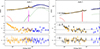 |
Fig. 1. Representative unfolded broadband X-ray spectra of NGC 1566 in type 1 and type 2 states (left and right panel, respectively). In the left panel, the orange and blue points represent the data from XMM-Newton/EPIC-PN and NuSTAR/FPMA observations, respectively. In the right panels, the black, orange, and blue points represent the Suzaku/XIS1, Suzaku/XIS0+XIS3, and Suzaku/HXD-PIN observations, respectively. The solid black, dot-dashed black, red dashed, solid magenta, and dotted green lines represent the total, continuum, soft excess, iron K-line, and reprocessed emission, respectively. The middle figures of each panel show the residual, while the data are fitted without the soft excess components. The bottom panels show the residuals for the full models. |
3.3. Eddington ratio and bolometric luminosity
Using Swift/UVOT and Swift/XRT observations, we studied the UV to X-ray SEDs using three component models: diskbb, blackbody, and cutoff power-law for disk, SE, and continuum emission, respectively. From the spectral modeling, we estimated the disk luminosity (Ldisk) in 10−7 − 0.5 keV, SE luminosity (LSE) in 0.001–10 keV, and continuum luminosity (LPL) in 0.1–500 keV. Then we calculated the bolometric luminosity as Lbol = Ldisk + LSE + LPL. When we had calculated Lbol, the Eddington ratio was estimated as λEdd = Lbol/LEdd, where LEdd = 1.5 × 1038(MBH/M⊙) erg s−1 is the Eddington luminosity. Our results are in good agreement with Gupta et al. (2024), who derived λEdd-dependent bolometric correction factors (κ2 − 10) from the SED analysis of unobscured AGNs in the BASS sample. The detailed SED fitting will be presented in a forthcoming publication.
3.4. Parameter estimation
We obtained several parameters from the spectral analysis, namely kTBB, Γ, Ecut, and Rf. We also calculated the SE flux ( ), continuum flux (
 ), and reflection flux (
 ), using the BLACKBODY component in the 0.5–2 keV range, CUTOFFPL in 2–10 keV, and PEXRAV in 10–40 keV, respectively. We chose the 0.5–2 keV energy range to represent
  as BLACKBODY with kTBB ∼ 0.1 − 0.2 keV is unlikely to contribute to the flux above 2 keV significantly. We represent the continuum emission in the 2–10 keV energy range, as this energy range has historically been used to present the continuum emission. As the reflection hump is generally observed to be most dominant in the ∼10–40 keV energy range, we used this energy range to represent
  .
.
We defined the soft excess strength (Q) as the ratio of the SE to the continuum luminosity:
 (1)
(1)
We also calculated the reflection strength as  .
.
Following Jana et al. (2025), we marked spectral type 1–1.5 as type 1 and type 1.8–2 as type 2 in this work. Since simultaneous optical spectra are scarce, we assigned the optical state of each observation based on the nearest available optical spectral classification. Figure 2 displays the light curve of all five CSAGNs in different panels. The blue circles and orange diamonds mark the type 1 and type 2 states, respectively. The vertical lines in each panel represent the optical observations. The solid horizontal lines in each panel represents the median of transition Eddington ratio,  at −2.01 ± 0.23 (from Jana et al. 2025). The dot-dashed horizontal lines represent the break-Eddington ratio in the V-shaped λEdd − Γ relation (
 , see Section 4.3 for details).
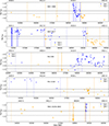 |
Fig. 2. Light curves of all five CSAGNs in different panels. The blue circles and orange diamonds mark the type 1 and type 2 states, respectively. The vertical lines in each panel represent the optical observations, where the solid blue and orange dot-dashed lines represent the type 1 and type 2 spectral states, respectively. The solid horizontal line in each panel represents the median of transition Eddington ratio |


We caution that some observations show type 2 state at high λEdd, while some exhibit type 1 state at low λEdd. This discrepancy may reflect the response time of the BLR to changes in the accretion rate. Moreover, the lack of simultaneous optical data for all X-ray observations may lead to misclassifications, especially during the state transitions.
3.5. Distribution of parameters
In our sample,  was found to be in the range ∼1041 − 1044 erg s−1. The median of
  for type 1 and type 2 states was found to be 42.89 ± 0.03 and 42.35 ± 0.16, respectively. The SE spanned four orders of magnitude, in the range ∼1039 − 43 erg s−1.
In several observations, only upper limits on the SE flux were available. For these, we performed 1000 Monte Carlo simulations by sampling the BLACKBODY normalization (NBB) uniformly between 0 and its upper limit, and computing the SE flux in each trial. The median was estimated using bootstrapping (see Ricci et al. 2018; Gupta et al. 2021, for details). The resulting median  values are 41.80 ± 0.07 and 40.72 ± 0.20 in the type 1 and type 2 states, respectively.
Figure 3 shows the distribution of kTBB, which lies in the ∼80 − 160 eV range and is similar across states, with medians at 122.5 ± 1.4 eV and 120.0 ± 0.1 eV in type 1 and type 2, respectively. The photon index (Γ) is obtained in range of ∼1.5 − 2.1, with medians of 1.72 ± 0.01 and 1.69 ± 0.02 in the type 1 and type 2 states, respectively.
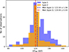 |
Fig. 3. Distribution of blackbody temperature (kTBB). The blue dashed and red dot-dashed lines represent the median value for the type 1 and type 2 states, respectively. |
log λEdd spans ∼ − 3.6 to −0.5 in our sample. The median of log λEdd for the two AGN types is obtained at −1.63 ± 0.06 and −2.67 ± 0.05, respectively. In type 1 log Q peaks around ∼ − 0.75 to −1.25, while in type 2 it is more evenly spread from ∼ − 2.4 to −1.25. Median values of log Q are −1.10 ± 0.03 and −1.73 ± 0.07 in the type 1 and type 2 states, respectively. The median values of all parameters are listed in Table 2.
Median of the X-ray spectral fit parameters.
To investigate the correlation between the different parameters, we used Spearman rank correlation. The correlation index and p-values are listed in Table 3. To investigate the correlations between the various parameters, we performed linear fitting in logarithmic space. To properly account for censored data, we employed a bootstrap approach. For each upper limit a random value was drawn from a uniform distribution between zero and the upper limit, and for each measured value a random sample was drawn from a Gaussian distribution using the measurement uncertainty as the standard deviation. This procedure produced a simulated dataset, which was fitted using LINMIX (Kelly et al. 2009) to obtain the best fit. The procedure was repeated 1000 times, and the average parameters were adopted as the final best-fit values.
Spearman correlation analysis result.
For visualization, we estimated binned medians using survival analysis with the SCIKIT-SURVIVAL package (Pölsterl 2020), which implements the Kaplan–Meier product limit (KMPL) estimator (Feigelson & Nelson 1985; Shimizu et al. 2017). This nonparametric method allows a robust estimation of median values in the presence of censored data. For each correlation, we computed KMPL-based medians in bins of the independent variable, ensuring at least 20 data points per bin.
4. Results and discussion
We studied five CSAGNs to investigate the origin of the SE and its relationship with primary continuum emission. As CSAGNs can show a wide range of λEdd on short timescales, we took advantage of CSAGNs to explore SE emission and its connection to the inner parts of the accretion flows in AGNs.
4.1. Soft excess temperature
We modeled the SE emission using a phenomenological blackbody component. From the spectral fits, we obtained the blackbody temperature (kTBB) for each observation. To investigate whether kTBB is related to the global properties of AGNs, we examined its dependence on several key parameters, namely Lbol,  ,
,  , Q, λEdd, and MBH. We found no statistically significant correlations between kTBB and any of these AGN parameters. The soft excess temperature remains remarkably uniform across a wide range of AGN properties, consistent with previous studies (e.g., Gierliński & Done 2004; Petrucci et al. 2018).
4.2. Primary continuum and soft excess relation
We find a strong positive correlation between SE and PC emission (p ≪ 10−10). Figure 4 displays the variation of  as a function of
  . Using linear regression analysis in logarithmic space, we obtained
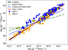 |
Fig. 4. Variation of the soft excess luminosity ( |


 (2)
(2)
with an intrinsic scatter of 0.22 dex. Here,  and
and  . We also obtained similar results for
  .
.
Previous studies have reported a strong positive correlation between SE and continuum flux in AGNs (e.g., Waddell & Gallo 2020; Nandi et al. 2023). Our fit yields a steep slope of ∼1.71, suggesting that SE emission increases more rapidly with PC emission than found in earlier works. For instance, Nandi et al. (2023) analyzed 20 unobscured AGNs and reported a shallower slope of 1.10 ± 0.04, using a power-law model over 0.5–10 keV. However, it is critical to note that their study used a power-law model to fit the SE component and considered the 0.5–10 keV energy range for both SE and PC emission. We converted those to 0.5–2 keV for the SE and 2–10 keV for the PC emission, for direct comparison with our work. By doing this, we obtained a revised slope of 0.77 ± 0.04, which is significantly flatter than the value we derived from our own sample of CSAGNs.
A similar trend is found for unobscured AGNs in the BASS sample (Jana et al., in prep.), which also uses a BLACKBODY model for the SE. The slope for BASS AGNs is 0.73 ± 0.04, still flatter than our sample of CSAGNs. These consistently flatter slopes across different AGN samples, are possibly due to differences in their accretion properties, black hole masses, or spectral modeling approaches. Furthermore, both Nandi et al. (2023) and Jana et al. (in prep.) mainly focused on type 1 AGNs with λEdd > 0.01, whereas our sample spans a broader range of λEdd (∼0.0003 − 0.3) and includes both type 1 and type 2 states.
To test the impact of AGN classification, we repeated our analysis using only CSAGNs in the type 1 state. The slope remains steep at 1.66 ± 0.21, which is consistent with the whole sample, and remains significantly steeper than the results of previous studies of type 1 AGNs. The strong SE-PC correlation across a large range of λEdd supports a common origin, possibly low-temperature Comptonization in a warm corona (e.g., Petrucci et al. 2018; Kubota & Done 2018).
4.3. Γ − λEdd relation and CS transitions
The Γ − λEdd relation provides important insights into AGN accretion and disk-corona coupling (Shemmer et al. 2006; Brightman et al. 2013; Yang et al. 2015; Trakhtenbrot et al. 2017, and references therein). Figure 5 shows this relation for our sample. A single-component linear fit of the form Γ = A + Blog λEdd fails to capture the observed trend. A two-component linear model with a break at  significantly improves the fit, indicating a fundamental change in the accretion properties of AGNs at this λEdd.
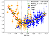 |
Fig. 5. Relation between Γ and λEdd. The blue circles and orange squares represent the data from the type 1 and type 2 states, respectively. The yellow stars represent the binned data points. The red lines represent the linear best fit of the dataset with a break at log λEdd = −2.47 ± 0.09. The break-point is marked by the vertical gray dashed line. The vertical green dash-dotted line represent the median of the transition Eddington ratio ( |


For  we found a positive correlation between Γ and λEdd, with a slope of 0.13 ± 0.07, indicating that AGNs in this regime exhibit a softer X-ray spectrum at higher accretion rates. This trend is consistent with findings obtained by previous studies focused on nearby BASS AGNs (e.g., Trakhtenbrot et al. 2017), which also reported a similar positive Γ–λEdd relation with a slope of ∼0.15 for log λEdd > −2.5. In contrast, for AGNs with
  , we observed a negative correlation, with a slope of −0.44 ± 0.11. We analyzed the variation of individual CSAGNs in our sample, which revealed a range of
  values, from 0.003 to 0.006 (see Appendix B). This variation in
  suggests that the transition in the Γ–λEdd relation is a general feature in CSAGNs and occurs around log λEdd ∼ –2 to –3.
Previous studies reported a possible V-shaped Γ − λEdd relation with breaks around log λEdd ∼ −2 to −2.5 (Gu & Cao 2009; She et al. 2018; Diaz et al. 2023). Recently, Diaz et al. (2023) studied a sample of low-luminosity AGNs and found a similar break at log λEdd ∼ −2.39, which closely matches our findings. She et al. (2018) also reported a break at log λEdd ∼ −2.5 while studying a sample of nearby AGNs with Chandra observations. The break observed in the Γ − λEdd relation is consistent with a transition between two distinct accretion states, similar to the hard to soft spectral state transitions observed in BHXBs (e.g., Remillard & McClintock 2006; Gu & Cao 2009; Jana et al. 2022). This is in agreement with theoretical expectations and recent observations, which suggest that CSAGNs are undergoing state transitions, analogous to the hard to soft transitions in BHXBs (e.g., Noda & Done 2018; Ross et al. 2018; Ruan et al. 2019; Ai et al. 2020; Yan et al. 2020; Hagen et al. 2024; Kang et al. 2025). In agreement with this idea, using a sample of AGNs that includes the sources analyzed here, Jana et al. (2025) showed that the median of transition Eddington ratio ( ; at which CSAGNs switch between type 1 and type 2 states) is
  , which is similar to
  .
.
4.4. Relation between soft excess and Eddington ratio
To understand how the SE emission changes in the variable objects studied here, we studied the dependence of Q (Eq. (1)) on different AGN parameters. Several studies suggest that SE emission varies with AGN properties, hinting at a close connection between SE and the accretion process (e.g., Boissay et al. 2016; Noda & Done 2018; Ghosh et al. 2022; Mehdipour et al. 2023; Nandi et al. 2023; Chen et al. 2025). In some cases, particularly at low flux levels, SE emission has been observed to disappear completely, suggesting a strong connection between SE strength and the accretion process (e.g., Noda & Done 2018; Ghosh et al. 2022).
We studied the dependence of Q on λEdd, a fundamental parameter thought to govern the physics of accretion in AGNs (e.g., Done et al. 2007; Ricci et al. 2018; Gupta et al. 2025). We find that as λEdd increases, the SE emission becomes significantly stronger. Figure 6 shows a strong positive correlation between Q and λEdd (p ≪ 10−10). The Q − λEdd relation is best described by a second-order polynomial fit,
![Mathematical equation: $$ \begin{aligned} \log Q&= (-0.078 \pm 0.019) [\log \lambda _{\rm Edd}]^2\nonumber \\&\qquad + (0.382 \pm 0.072) \log \lambda _{\rm Edd} - (0.339 \pm 0.088), \end{aligned} $$](/articles/aa/full_html/2026/03/aa56654-25/aa56654-25-eq46.gif) (3)
(3)
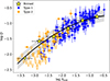 |
Fig. 6. Soft excess strength (Q) as a function of Eddington ratio (λEdd). The filled blue circles and orange squares represent the data from type 1 and type 2 states, respectively, while the open blue circles and orange squares represent the upper limits from type 1 and type 2 state, respectively. The yellow stars represent the binned data points, while the yellow down triangle represents the upper limit. The black dashed line represents the best fit. The gray region marks the 1σ scatter. |
with an intrinsic scatter of 0.19 dex.
A positive correlation between Q and λEdd was originally reported by Boissay et al. (2016) for a sample of 102 hard X-ray selected Seyfert 1 galaxies, although with a very large scatter and flatter slope. Similarly, Waddell & Gallo (2020) suggested the presence of this trend for broad-line Seyfert 1 (BLS1) galaxies, but found that the correlation weakens for narrow-line Seyfert 1 (NLS1) galaxies, which are typically high λEdd sources. Unlike these studies, our sample includes lower-luminosity AGNs, enabling us to probe SE behavior at λEdd < 0.01. In this regime, Q declines sharply, and in many cases the soft excess is not detected, indicating that SE emission weakens or disappears at very low accretion rates. A similar behavior has also been observed in some AGNs where SE emission weakens at the low-accretion state (e.g., Noda & Done 2018; Hagen et al. 2024; Chen et al. 2025).
The Q − λEdd trend we find supports a scenario in which SE emission is closely linked to the inner accretion flow and corona. In both warm Comptonization and blurred reflection scenarios one could expect an enhanced SE at higher λEdd due to increased disk ionization and/or density. For more details, see Sect. 2.9 of the Language Guide. or more efficient disk-corona coupling. In the reflection scenario, at low λEdd, the disk may recede and the corona may expand, reducing the reprocessing efficiency, and thus the SE emission (e.g., Reis & Miller 2013; Done et al. 2007; Wilkins et al. 2016). At high accretion rates, the disk would be more ionized, with an inner radius closer to the ISCO, resulting in stronger reflection. On the other hand, in the warm Comptonization scenario at low λEdd, the warm corona may become inefficient or the inner accretion disk may transition to a radiatively inefficient flow, leading to the suppression or disappearance of the soft excess emission (e.g., Mehdipour et al. 2023; Layek et al. 2024). The disappearance or weakening of SE emission at very low λEdd suggests that at λEdd < 0.01 the conditions required to produce SE are no longer sustained.
4.5. The relation between soft excess and Compton hump
To quantify the influence of the Compton hump, we parameterized it using the reflection strength (RS). Figure 7 illustrates the variation of RS as a function of Q. We did not find any significant correlation between these two quantities, with a p-value of 0.83, suggesting that the reflection strength in CSAGNs is not strongly dependent on Q. If the SE originates primarily from blurred reflection, a positive correlation between Q and RS is expected (e.g., Vasudevan et al. 2014; Boissay et al. 2016). However, our results do not support this scenario, which implies that SE and reflection arise from different physical processes. A study by Waddell & Gallo (2020) found a positive correlation between Q and the hard X-ray excess (similar to RS) in a sample of NLS1 galaxies, but no correlation in BLS1 galaxies. The authors suggested that in NLS1s, SE originates from reflection, whereas in BLS1s, alternative mechanisms such as warm Comptonization or ionized absorption may be responsible.
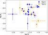 |
Fig. 7. Soft excess strength (Q) as a function of reflection strength (RS). The blue circles and orange squares represent the data from type 1 and type 2 states, respectively. |
We note that the neutral reflection from the torus and BLR also could contribute to the Compton hump, along with the reflection from the disk. The reflection properties of our sample were extensively investigated in previous studies, which consistently report very weak or negligible reflection signatures (e.g., Parker et al. 2019; Jana et al. 2021; Ghosh et al. 2022; Tripathi & Dewangan 2022; Veronese et al. 2024). In many cases, the spectra can be adequately modeled without requiring any reflection component. Even if the torus or the BLR contributes to the Compton hump, the contribution is minimal, and the overall Compton hump flux (torus + ionized disk) remains weak. The combination of a strong SE and weak or absent Compton hump disfavors ionized reflection as the dominant origin of the SE.
4.6. Soft excess and photon index relation
We explored the relationship between Γ and Q for our sample and found a V-shaped Γ − Q relation (Figure 8), similar to the relation between Γ and λEdd. A Spearman correlation analysis yielded a correlation coefficient of −0.22 with p = 0.33 for log Q < −1.53, and 0.71 with p ≪ 10−5 for log Q > −1.53. Given the strong correlation between Q and λEdd, the presence of this break is expected.
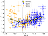 |
Fig. 8. Relation between photon index (Γ) and the soft excess strength (Q) is shown. The blue circles and orange squares represent the data from type 1 and type 2 states, respectively. The open blue circles and orange squares represent the upper limit from type 1 and type 2 states, respectively. The yellow stars represent the binned data points. The black solid lines represent the linear best fit of the dataset with a break at log Q = −1.62 ± 0.12, which corresponds to log λEdd = −2.60 ± 0.14. The break-point is marked by the vertical black dashed line. |
Boissay et al. (2016) found a positive correlation between Q and Γ. Their sample consisted of AGNs with log λEdd > −2.2, and therefore our findings for log Q > −1.53 (corresponding to log λEdd ∼ −2.6) are consistent with their results. Additionally, Boissay et al. (2016) predicted a weak negative correlation between Γ and Q under an ionized reflection scenario using simulations carried out with the relxillp_ion model. As the result of this study is consistent with the finding of Boissay et al. (2016), our findings are inconsistent with the ionized reflection scenario for log λEdd > −2.6. For log Q < −1.53 (i.e., log λEdd < −2.2), no correlation is observed between Γ and Q, as we mostly observed an upper limit of Q. This suggests that, in this accretion regime, the warm corona may not be linked to the hot corona or it becomes extremely weak.
4.7. The origin of the soft excess
The soft excess remains a long-standing puzzle four decades after its discovery (Arnaud et al. 1985; Singh et al. 1985). Understanding the physical mechanisms responsible for the SE is crucial, as it directly impacts our understanding of accretion processes in AGNs. In the ionized reflection scenario, SE arises from reflection off an ionized AD close to the SMBH. Several studies, including those of Vasudevan et al. (2014) and Boissay et al. (2016), have predicted specific correlations between spectral parameters within this framework. While a positive correlation between RS and Q, as well as a negative correlation between Γ and Q, are expected, we find no such trends (see Figs. 8 and 7). Moreover, our broadband spectra show weak or absent Compton humps, a key signature of reflection-dominated spectra (Ross & Fabian 2005; Walton et al. 2013). The absence of strong reprocessed emission across a wide range of λEdd further weakens the case for ionized reflection as the primary SE mechanism. This aligns with the findings of previous studies, which indicate that while ionized reflection can contribute to the SE in certain AGNs, it is unlikely to be the main mechanism producing this component (Gallo et al. 2019; Nandi et al. 2023).
In contrast, our results show a tight correlation between SE and continuum flux (see Fig. 4) across a wide range of λEdd, favoring warm Comptonization. The tight Q − λEdd relation (see Fig. 5) implies that SE emission closely tracks accretion activity, consistent with models where UV disk photons are up-scattered in a warm, optically thick corona (Crummy et al. 2006; Done et al. 2012; Kubota & Done 2018; Middei et al. 2020). Recently, Palit et al. (2024) suggested that the warm corona size increases with λEdd, enhancing SE emission (see also Chen et al. 2025), which is consistent with our findings.
Our study aligns with recent studies of CSAGNs, which suggest that warm Comptonization is the most likely origin for the SE (Jana et al. 2021; Tripathi & Dewangan 2022; Giustini et al. 2017; Veronese et al. 2024). For Mrk 590, Laha et al. (2022) found that both warm Comptonization and ionized reflection could fit the data. However, our analysis favors warm Comptonization as the leading explanation for SE in our sample. While ionized reflection can become significant in highly accreting AGNs (λEdd ∼ 1), this regime is beyond the scope of our study and will be explored in future works. Our results add to the growing consensus that warm Comptonization is a key mechanism shaping the soft X-ray excess in AGNs, especially in systems with moderate to low accretion rates (λEdd = 0.001 − 0.3).
4.8. SE and CS transitions
The SE is believed to play a central role in regulating the ionization state of the BLR, with changes in its flux capable of substantially modifying the ionizing photon budget (Noda & Done 2018). Recent studies have shown that during CS transitions, the SE flux often varies more dramatically than the PC emission, suggesting a strong connection between SE variability and changes in AGN state (e.g., Noda & Done 2018; Mehdipour et al. 2022a). For our sample, we find that the median SE and PC luminosities in the type 1 state are ∼6.3 × 1041 erg s−1 and ∼7.8 × 1042 erg s−1, respectively. In contrast, during the type 2 state, the corresponding median values drop to ∼5.2 × 1040 erg s−1 and ∼2.2 × 1042 erg s−1. This corresponds to a factor of ∼12 change in the SE and a factor of ∼3.5 in the PC between the two states, further indicating that the SE exhibits stronger variability across CS transitions. Except for IRAS 23226–3843, the median SE luminosity changes more drastically than the PC luminosity between spectral states for all sources in our sample. This trend is consistent with the broader picture in which a decline in accretion rate reduces the extreme ultraviolet continuum, leading to fewer ionizing photons and, consequently, weaker or absent BELs (Noda & Done 2018; Ruan et al. 2019). Our finding is consistent with the previous studies of CSAGNs. For instance, in NGC 1566, the SE and PC increased by factors of ∼200 and ∼30, respectively, as the source transitioned from a type 2 to a type 1 state (Tripathi & Dewangan 2022). A similar trend has been observed in Mrk 1018, where the SE exhibited stronger variability than the PC across spectral transitions (Noda & Done 2018; Saha et al. 2025).
This trend is not restricted to a few rare CSAGNs, but is observed in the general AGN population. A few studies showed a sharp decline in the fraction of broad-line AGNs below λEdd ∼ 0.01 − 0.02 (Trump et al. 2011; Mitchell et al. 2023; Hagen et al. 2024; Kang et al. 2025), which coincides with the transition Eddington ratio for CSAGNs. Additionally, we find that the median Q, is ∼0.08 in the type 1 state and ∼0.02 in the type 2 state. This result is consistent with the interpretation that the SE diminishes more rapidly than the PC as AGNs transition to type 2 states. The strong dependence of both Q and SE luminosity on spectral state suggests that the SE is intrinsically connected to CS transitions (Noda & Done 2018). Table 4 shows how the median values of different parameters change between the type 1 and type 2 states.
Factor of change in the median value of fluxes and soft excess strength between type 1 & type 2 states.
5. Summary and conclusions
We investigated the X-ray properties of a sample of five CSAGNs to understand the nature of their inner accretion flow, soft excess emission, and their connection to CS transitions. We used a total 42 XMM-Newton, 4 Suzaku, 22 NuSTAR, and 1021 Swift/XRT observations for our study. Our sample spans three orders of magnitude in Eddington ratios (λEdd ∼ 0.0003 − 0.3) and covers both type 1 and type 2 states. Based on the broadband X-ray spectral study, we retrieved several accretion parameters, namely photon index, blackbody temperature, soft excess strength, soft excess, and primary continuum luminosity. On the basis of multiple correlations, our findings suggest that SE emission originates from a warm corona across a broad range of accretion rates. In the following, we summarize our key findings:
-
We find that SE and PC emission are tightly correlated, with an intrinsic scatter of 0.22 dex (1σ) over four orders of magnitude in luminosity (Fig. 4). The soft excess luminosities cover a wider range than primary continuum luminosities, indicating that the SE is more variable than the continuum emission.
-
The SE emission in CSAGNs varies more rapidly than in AGNs that do not undergo CS transitions. The steeper slope in the SE-PC relation for CSAGNs suggests that these objects experience more pronounced spectral variations, possibly driven by rapid changes in the accretion rate. We also found that the SE emission changes more compared to the PC emission during the CS transitions, suggesting that the SE is intrinsically connected to the optical state change.
-
We observed a very clear V-shaped Γ − λEdd relation with a break at log λEdd = −2.47 ± 0.09 (Fig. 5). This break is consistent with
 for changing-state transitions, which is generally observed at
  .
. -
The soft excess strength correlates positively with λEdd (Fig. 6), indicating that SE emission increases significantly in high-accretion states. This suggests a close connection between SE and the inner accretion disk.
-
We find no correlation between Q and the reflection strength (Fig. 7); this suggests that SE emission is not dominated by blurred reflection.
-
At high accretion rates (λEdd > 0.001), Q and Γ exhibit a positive correlation (Fig. 8).
Overall, from our sample, we find that the warm Comptonization scenario is the most likely origin of the SE, at least in the range of λEdd probed here (λEdd ∼ 0.003 − 0.3). CSAGNs offer crucial insight into the structure and evolution of the inner accretion flow in SMBHs. Our results indicate that SE emission is closely linked to the continuum and is likely dominated by warm Comptonization. This warm coronal emission appears tightly connected to the accretion disk, which radiates primarily in the UV/optical. In a forthcoming study, we will present the UV/optical to X-ray SED to further explore this connection.
Future work will extend the analysis to higher λEdd AGNs (Kallova et al., in prep.; Kumari et al., in prep.) to examine warm Comptonization under different accretion regimes. We find that SE varies more rapidly than the PC during state transitions. Follow-up studies will explore the connection between SE and BELs to understand the physical drivers of BELs using multiwavelength data. To deepen our understanding of SE and its link to the primary X-ray continuum, future studies with larger AGN samples and high-resolution X-ray spectroscopy will be essential. Missions such as XPOSAT (Paul 2022; Vatedka et al. 2025) and NewAthena (Cruise et al. 2025) will help constrain the physical mechanisms behind SE. Additionally, proposed observatories such as AXIS (Reynolds et al. 2023) will be critical for building a comprehensive model of AGN accretion physics and X-ray emission evolution across AGN populations.
Data availability
All the data used in the paper are publicly available. The data are available at the CDS via https://cdsarc.cds.unistra.fr/viz-bin/cat/J/A+A/707/A213
Acknowledgments
We acknowledge support from ANID grants FONDECYT Postdoctoral fellowship 3230303 (AJ) and 3230310 (YD), ANID-Chile BASAL CATA FB210003 (FEB), FONDECYT Regular 1241005 (FEB), and the Millennium Science Initiative, AIM23-0001 (FEB). C.R.acknowledges support from SNSF Consolidator grant F01–13252, Fondecyt Regular grant 1230345, ANID BASAL project FB210003 and the China-Chile joint research fund. A.T. acknowledges financial support from the Bando Ricerca Fondamentale INAF 2022 Large Grant “Toward an holistic view of the Titans: multiband observations of z > 6 QSOs powered by greedy supermassive black holes”. B.T. acknowledges support from the European Research Council (ERC) under the European Union’s Horizon 2020 research and innovation program (grant agreement number 950533). This research was supported by the Excellence Cluster ORIGINS which is funded by the Deutsche Forschungsgemeinschaft (DFG, German Research Foundation) under Germany’s Excellence Strategy – EXC 2094 – 390783311. B.T. also acknowledges the hospitality of the Instituto de Estudios Astrofísicos at Universidad Diego Portales, the Instituto de Astrofísica at Pontificia Universidad Católica de Chile, and the Institut d’Astrophysique de Paris, where parts of this study have been carried out. MJT acknowledges support from UKRI ST/X001075/1. M.K. acknowledges support from NASA through ADAP award 80NSSC22K1126. KKG acknowledges financial support from the Belgian Federal Science Policy Office (BELSPO) in the framework of the PRODEX Programme of the European Space Agency. HKC acknowledges supports the grant NSTC 113-2112-M-007-020. D.I. acknowledges funding provided by the University of Belgrade, Faculty of Mathematics (the contract 451-03-136/2025-03/200104) through the grants by the Ministry of Science, Technological Development and Innovation of the Republic of Serbia. E.S. acknowledges the support of the Alexander von Humboldt Foundation. This research has made use of data and/or software provided by the High Energy Astrophysics Science Archive Research Center (HEASARC), which is a service of the Astrophysics Science Division at NASA/GSFC and the High Energy Astrophysics Division of the Smithsonian Astrophysical Observatory. This work has made use of data obtained from the NuSTAR mission, a project led by Caltech, funded by NASA and managed by NASA/JPL, and has utilized the NuSTARDAS software package, jointly developed by the ASDC, Italy and Caltech, USA. This research has made use of observations obtained with XMM–Newton, an ESA science mission with instruments and contributions directly funded by ESA Member States and NASA. This work made use of XRT data supplied by the UK Swift Science Data Centre at the University of Leicester, UK. This work has made use of data obtained from Suzaku, a collaborative mission between the space agencies of Japan (JAXA) and the USA (NASA).
References
- Ai, Y., Dou, L., Yang, C., et al. 2020, ApJ, 890, L29 [NASA ADS] [CrossRef] [Google Scholar]
- Arnaud, K. A. 1996, ASP Conf. Ser., 101, 17 [Google Scholar]
- Arnaud, K. A., Branduardi-Raymont, G., Culhane, J. L., et al. 1985, MNRAS, 217, 105 [NASA ADS] [CrossRef] [Google Scholar]
- Beuchert, T., Markowitz, A. G., Dauser, T., et al. 2017, A&A, 603, A50 [NASA ADS] [CrossRef] [EDP Sciences] [Google Scholar]
- Boissay, R., Ricci, C., & Paltani, S. 2016, A&A, 588, A70 [NASA ADS] [CrossRef] [EDP Sciences] [Google Scholar]
- Brightman, M., Silverman, J. D., Mainieri, V., et al. 2013, MNRAS, 433, 2485 [Google Scholar]
- Burrows, D. N., Hill, J. E., Nousek, J. A., et al. 2005, Space Sci. Rev., 120, 165 [Google Scholar]
- Chakrabarti, S., & Titarchuk, L. G. 1995, ApJ, 455, 623 [NASA ADS] [CrossRef] [Google Scholar]
- Chen, S.-J., Wang, J.-X., Kang, J.-L., et al. 2025, ApJ, 980, 23 [Google Scholar]
- Chen, S.-J., Buchner, J., Liu, T., et al. 2025, A&A, 701, A144 [NASA ADS] [CrossRef] [EDP Sciences] [Google Scholar]
- Cohen, R. D., Rudy, R. J., Puetter, R. C., Ake, T. B., & Foltz, C. B. 1986, ApJ, 311, 135 [NASA ADS] [CrossRef] [Google Scholar]
- Cruise, M., Guainazzi, M., Aird, J., et al. 2025, Nat. Astron., 9, 36 [Google Scholar]
- Crummy, J., Fabian, A. C., Gallo, L., & Ross, R. R. 2006, MNRAS, 365, 1067 [Google Scholar]
- Dauser, T., Garcia, J., Parker, M. L., Fabian, A. C., & Wilms, J. 2014, MNRAS, 444, L100 [Google Scholar]
- Dauser, T., García, J., Walton, D. J., et al. 2016, A&A, 590, A76 [NASA ADS] [CrossRef] [EDP Sciences] [Google Scholar]
- Denney, K. D., De Rosa, G., Croxall, K., et al. 2014, ApJ, 796, 134 [Google Scholar]
- Diaz, Y., Hernàndez-García, L., Arévalo, P., et al. 2023, A&A, 669, A114 [NASA ADS] [CrossRef] [EDP Sciences] [Google Scholar]
- Ding, Y., Garcıa, J. A., Kallman, T. R., et al. 2024, ApJ, 974, 280 [Google Scholar]
- Done, C., Gierliński, M., & Kubota, A. 2007, A&ARv, 15, 1 [Google Scholar]
- Done, C., Davis, S. W., Jin, C., Blaes, O., & Ward, M. 2012, MNRAS, 420, 1848 [Google Scholar]
- Edelson, R., Gelbord, J., Cackett, E., et al. 2017, ApJ, 840, 41 [NASA ADS] [CrossRef] [Google Scholar]
- Emmanoulopoulos, D., Papadakis, I. E., McHardy, I. M., et al. 2012, MNRAS, 424, 1327 [Google Scholar]
- Esin, A. A., McClintock, J. E., & Narayan, R. 1997, ApJ, 489, 865 [NASA ADS] [CrossRef] [Google Scholar]
- Evans, P. A., Beardmore, A. P., Page, K. L., et al. 2009, MNRAS, 397, 1177 [Google Scholar]
- Feigelson, E. D., & Nelson, P. I. 1985, ApJ, 293, 192 [NASA ADS] [CrossRef] [Google Scholar]
- Fender, R., & Belloni, T. 2004, ARA&A, 42, 317 [NASA ADS] [CrossRef] [Google Scholar]
- Feng, H.-C., Liu, H. T., Bai, J. M., et al. 2021, ApJ, 912, 92 [NASA ADS] [CrossRef] [Google Scholar]
- Frank, J., King, A., & Raine, D. J. 2002, Accretion Power in Astrophysics (Third Edition (Cambridge University Press)) [Google Scholar]
- Fukazawa, Y., Mizuno, T., Watanabe, S., et al. 2009, PASJ, 61, S17 [Google Scholar]
- Gallo, L. C., Gonzalez, A. G., Waddell, S. G. H., et al. 2019, MNRAS, 484, 4287 [Google Scholar]
- García, J., & Kallman, T. R. 2010, ApJ, 718, 695 [CrossRef] [Google Scholar]
- García, J. A., Kara, E., Walton, D., et al. 2019, ApJ, 871, 88 [CrossRef] [Google Scholar]
- Ghosh, R., Laha, S., Deshmukh, K., et al. 2022, ApJ, 937, 31 [Google Scholar]
- Gierliński, M., & Done, C. 2004, MNRAS, 349, L7 [Google Scholar]
- Giustini, M., Costantini, E., De Marco, B., et al. 2017, A&A, 597, A66 [NASA ADS] [CrossRef] [EDP Sciences] [Google Scholar]
- Gruber, D. E., Matteson, J. L., Peterson, L. E., & Jung, G. V. 1999, ApJ, 520, 124 [NASA ADS] [CrossRef] [Google Scholar]
- Gu, M., & Cao, X. 2009, MNRAS, 399, 349 [NASA ADS] [CrossRef] [Google Scholar]
- Gupta, K. K., Ricci, C., Tortosa, A., et al. 2021, MNRAS, 504, 428 [NASA ADS] [CrossRef] [Google Scholar]
- Gupta, K. K., Ricci, C., Temple, M. J., et al. 2024, A&A, 691, A203 [NASA ADS] [CrossRef] [EDP Sciences] [Google Scholar]
- Gupta, K. K., Ricci, C., Tortosa, A., et al. 2025, ApJ, 990, 86 [Google Scholar]
- Haardt, F., & Maraschi, L. 1991, ApJ, 380, L51 [Google Scholar]
- Hagen, S., Done, C., Silverman, J. D., et al. 2024, MNRAS, 534, 2803 [NASA ADS] [CrossRef] [Google Scholar]
- Harrison, F. A., Craig, W. W., Christensen, F. E., et al. 2013, ApJ, 770, 103 [Google Scholar]
- Jana, A., Kumari, N., Nandi, P., et al. 2021, MNRAS, 507, 687 [NASA ADS] [CrossRef] [Google Scholar]
- Jana, A., Ricci, C., Naik, S., et al. 2022, MNRAS, 512, 5942 [CrossRef] [Google Scholar]
- Jana, A., Ricci, C., Temple, M. J., et al. 2025, A&A, 693, A35 [NASA ADS] [CrossRef] [EDP Sciences] [Google Scholar]
- Jansen, F., Lumb, D., Altieri, B., et al. 2001, A&A, 365, L1 [NASA ADS] [CrossRef] [EDP Sciences] [Google Scholar]
- Kang, J.-L., Done, C., Hagen, S., et al. 2025, MNRAS, 538, 121 [Google Scholar]
- Kawamuro, T., Ueda, Y., Tazaki, F., & Terashima, Y. 2013, ApJ, 770, 157 [NASA ADS] [CrossRef] [Google Scholar]
- Kelly, B. C., Bechtold, J., & Siemiginowska, A. 2009, ApJ, 698, 895 [Google Scholar]
- Kollatschny, W., Grupe, D., Parker, M. L., et al. 2020, A&A, 638, A91 [NASA ADS] [CrossRef] [EDP Sciences] [Google Scholar]
- Kollatschny, W., Grupe, D., Parker, M. L., et al. 2023, A&A, 670, A103 [NASA ADS] [CrossRef] [EDP Sciences] [Google Scholar]
- Koratkar, A., Deustua, S. E., Heckman, T., et al. 1995, ApJ, 440, 132 [NASA ADS] [CrossRef] [Google Scholar]
- Koss, M. J., Ricci, C., Trakhtenbrot, B., et al. 2022a, ApJS, 261, 2 [NASA ADS] [CrossRef] [Google Scholar]
- Koss, M. J., Trakhtenbrot, B., Ricci, C., et al. 2022b, ApJS, 261, 6 [NASA ADS] [CrossRef] [Google Scholar]
- Koyama, K., Tsunemi, H., Dotani, T., et al. 2007, PASJ, 59, 23 [Google Scholar]
- Krolik, J. H. 1999, Active Galactic Nuclei: From the Central Black Hole to the Galactic Environment (Princeton University Press) [Google Scholar]
- Kubota, A., & Done, C. 2018, MNRAS, 480, 1247 [Google Scholar]
- Laha, S., Meyer, E., Roychowdhury, A., et al. 2022, ApJ, 931, 5 [NASA ADS] [CrossRef] [Google Scholar]
- Lawther, D., Vestergaard, M., Raimundo, S., et al. 2023, MNRAS, 519, 3903 [Google Scholar]
- Layek, N., Nandi, P., Naik, S., et al. 2024, MNRAS, 528, 5269 [NASA ADS] [CrossRef] [Google Scholar]
- Lu, K.-X., Li, Y.-R., Wu, Q., et al. 2025, ApJS, 276, 51 [Google Scholar]
- Lyu, B., Yan, Z., Yu, W., & Wu, Q. 2021, MNRAS, 506, 4188 [NASA ADS] [CrossRef] [Google Scholar]
- Maccarone, T. J. 2003, A&A, 409, 697 [NASA ADS] [CrossRef] [EDP Sciences] [Google Scholar]
- MacLeod, C. L., Ross, N. P., Lawrence, A., et al. 2016, MNRAS, 457, 389 [Google Scholar]
- Magdziarz, P., Blaes, O. M., Zdziarski, A. A., Johnson, W. N., & Smith, D. A. 1998, MNRAS, 301, 179 [NASA ADS] [CrossRef] [Google Scholar]
- Malkan, M. A., & Sargent, W. L. W. 1982, ApJ, 254, 22 [NASA ADS] [CrossRef] [Google Scholar]
- McElroy, R. E., Husemann, B., Croom, S. M., et al. 2016, A&A, 593, L8 [NASA ADS] [CrossRef] [EDP Sciences] [Google Scholar]
- McHardy, I. M., Koerding, E., Knigge, C., Uttley, P., & Fender, R. P. 2006, Nature, 444, 730 [NASA ADS] [CrossRef] [Google Scholar]
- Mehdipour, M., Kriss, G. A., Brenneman, L. W., et al. 2022a, ApJ, 925, 84 [NASA ADS] [CrossRef] [Google Scholar]
- Mehdipour, M., Kriss, G. A., Costantini, E., et al. 2022b, ApJ, 934, L24 [NASA ADS] [CrossRef] [Google Scholar]
- Mehdipour, M., Kriss, G. A., Kaastra, J. S., Costantini, E., & Mao, J. 2023, ApJ, 952, L5 [NASA ADS] [CrossRef] [Google Scholar]
- Merloni, A., Heinz, S., & di Matteo, T. 2003, MNRAS, 345, 1057 [Google Scholar]
- Merloni, A., Dwelly, T., Salvato, M., et al. 2015, MNRAS, 452, 69 [Google Scholar]
- Middei, R., Petrucci, P. O., Bianchi, S., et al. 2020, A&A, 640, A99 [NASA ADS] [CrossRef] [EDP Sciences] [Google Scholar]
- Mitchell, J. A. J., Done, C., Ward, M. J., et al. 2023, MNRAS, 524, 1796 [NASA ADS] [CrossRef] [Google Scholar]
- Nandi, P., Chatterjee, A., Jana, A., et al. 2023, ApJS, 269, 15 [Google Scholar]
- Netzer, H. 2013, The Physics and Evolution of Active Galactic Nuclei (Cambridge University Press) [Google Scholar]
- Noda, H., & Done, C. 2018, MNRAS, 480, 3898 [Google Scholar]
- Ochmann, M. W., Kollatschny, W., & Zetzl, M. 2020, Contrib. Astron. Obs. Skalnate Pleso, 50, 318 [NASA ADS] [Google Scholar]
- Ochmann, M. W., Kollatschny, W., Probst, M. A., et al. 2024, A&A, 686, A17 [NASA ADS] [CrossRef] [EDP Sciences] [Google Scholar]
- Oh, K., Koss, M. J., Ueda, Y., et al. 2022, ApJS, 261, 4 [NASA ADS] [CrossRef] [Google Scholar]
- Oknyansky, V. L., Gaskell, C. M., Huseynov, N. A., et al. 2017, MNRAS, 467, 1496 [NASA ADS] [Google Scholar]
- Oknyansky, V. L., Winkler, H., Tsygankov, S. S., et al. 2019, MNRAS, 483, 558 [NASA ADS] [CrossRef] [Google Scholar]
- Oknyansky, V. L., Tsygankov, S. S., Dodin, A. S., et al. 2023, ATel, 16324, 1 [Google Scholar]
- Palit, B., Różańska, A., Petrucci, P. O., et al. 2024, A&A, 690, A308 [NASA ADS] [CrossRef] [EDP Sciences] [Google Scholar]
- Palit, B., Śniegowska, M., Markowitz, A., et al. 2025, MNRAS, 540, L14 [Google Scholar]
- Panda, S., & Śniegowska, M. 2024, ApJS, 272, 13 [NASA ADS] [CrossRef] [Google Scholar]
- Parker, M. L., Schartel, N., Grupe, D., et al. 2019, MNRAS, 483, L88 [NASA ADS] [CrossRef] [Google Scholar]
- Paul, B. 2022, in 44th COSPAR Scientific Assembly. Held 16–24 July, 44, 1853 [Google Scholar]
- Peca, A., Koss, M. J., Oh, K., et al. 2025, ApJ, 990, 3 [Google Scholar]
- Petrucci, P. O., Paltani, S., Malzac, J., et al. 2013, A&A, 549, A73 [NASA ADS] [CrossRef] [EDP Sciences] [Google Scholar]
- Petrucci, P. O., Ursini, F., De Rosa, A., et al. 2018, A&A, 611, A59 [NASA ADS] [CrossRef] [EDP Sciences] [Google Scholar]
- Pölsterl, S. 2020, J. Mach. Learn. Res., 21, 1 [Google Scholar]
- Rees, M. J. 1988, Nature, 333, 523 [Google Scholar]
- Reis, R. C., & Miller, J. M. 2013, ApJ, 769, L7 [NASA ADS] [CrossRef] [Google Scholar]
- Remillard, R. A., & McClintock, J. E. 2006, ARA&A, 44, 49 [Google Scholar]
- Reynolds, C. S., Kara, E. A., Mushotzky, R. F., et al. 2023, SPIE Conf. Ser., 12678, 126781E [Google Scholar]
- Ricci, C., & Trakhtenbrot, B. 2023, Nat. Astron., 7, 1282 [Google Scholar]
- Ricci, C., Trakhtenbrot, B., Koss, M. J., et al. 2017, ApJS, 233, 17 [Google Scholar]
- Ricci, C., Ho, L. C., Fabian, A. C., et al. 2018, MNRAS, 480, 1819 [NASA ADS] [CrossRef] [Google Scholar]
- Ricci, C., Kara, E., Loewenstein, M., et al. 2020, ApJ, 898, L1 [Google Scholar]
- Ricci, C., Loewenstein, M., Kara, E., et al. 2021, ApJS, 255, 7 [NASA ADS] [CrossRef] [Google Scholar]
- Risaliti, G., Elvis, M., Fabbiano, G., Baldi, A., & Zezas, A. 2005, ApJ, 623, L93 [Google Scholar]
- Risaliti, G., Salvati, M., Elvis, M., et al. 2009, MNRAS, 393, L1 [NASA ADS] [CrossRef] [Google Scholar]
- Rivers, E., Markowitz, A., Duro, R., & Rothschild, R. 2012, ApJ, 759, 63 [NASA ADS] [CrossRef] [Google Scholar]
- Ross, R. R., & Fabian, A. C. 2005, MNRAS, 358, 211 [CrossRef] [Google Scholar]
- Ross, N. P., Ford, K. E. S., Graham, M., et al. 2018, MNRAS, 480, 4468 [Google Scholar]
- Ruan, J. J., Anderson, S. F., Eracleous, M., et al. 2019, ApJ, 883, 76 [NASA ADS] [CrossRef] [Google Scholar]
- Saha, T., Krumpe, M., Markowitz, A., et al. 2025, A&A, 699, A205 [NASA ADS] [CrossRef] [EDP Sciences] [Google Scholar]
- Shakura, N. I., & Sunyaev, R. A. 1973, A&A, 500, 33 [NASA ADS] [Google Scholar]
- Shappee, B. J., Prieto, J. L., Grupe, D., et al. 2014, ApJ, 788, 48 [Google Scholar]
- She, R., Ho, L. C., Feng, H., & Cui, C. 2018, ApJ, 859, 152 [NASA ADS] [CrossRef] [Google Scholar]
- Shemmer, O., Brandt, W. N., Netzer, H., Maiolino, R., & Kaspi, S. 2006, ApJ, 646, L29 [Google Scholar]
- Sheng, Z., Wang, T., Jiang, N., et al. 2017, ApJ, 846, L7 [NASA ADS] [CrossRef] [Google Scholar]
- Shimizu, T. T., Mushotzky, R. F., Meléndez, M., et al. 2017, MNRAS, 466, 3161 [NASA ADS] [CrossRef] [Google Scholar]
- Sikora, M., Stawarz, Ł., & Lasota, J.-P. 2007, ApJ, 658, 815 [NASA ADS] [CrossRef] [Google Scholar]
- Singh, K. P., Garmire, G. P., & Nousek, J. 1985, ApJ, 297, 633 [NASA ADS] [CrossRef] [Google Scholar]
- Sobolewska, M. A., Siemiginowska, A., & Gierliński, M. 2011, MNRAS, 413, 2259 [CrossRef] [Google Scholar]
- Stern, D., McKernan, B., Graham, M. J., et al. 2018, ApJ, 864, 27 [Google Scholar]
- Sunyaev, R. A., & Titarchuk, L. G. 1980, A&A, 500, 167 [NASA ADS] [Google Scholar]
- Svoboda, J., Guainazzi, M., & Merloni, A. 2017, A&A, 603, A127 [NASA ADS] [CrossRef] [EDP Sciences] [Google Scholar]
- Takahashi, T., Abe, K., Endo, M., et al. 2007, PASJ, 59, 35 [Google Scholar]
- Temple, M. J., Ricci, C., Koss, M. J., et al. 2023, MNRAS, 518, 2938 [Google Scholar]
- Trakhtenbrot, B., Ricci, C., Koss, M. J., et al. 2017, MNRAS, 470, 800 [NASA ADS] [CrossRef] [Google Scholar]
- Trakhtenbrot, B., Arcavi, I., MacLeod, C. L., et al. 2019, ApJ, 883, 94 [Google Scholar]
- Tripathi, P., & Dewangan, G. C. 2022, ApJ, 930, 117 [NASA ADS] [CrossRef] [Google Scholar]
- Trump, J. R., Impey, C. D., Kelly, B. C., et al. 2011, ApJ, 733, 60 [NASA ADS] [CrossRef] [Google Scholar]
- Vasudevan, R. V., & Fabian, A. C. 2007, MNRAS, 381, 1235 [NASA ADS] [CrossRef] [Google Scholar]
- Vasudevan, R. V., Mushotzky, R. F., Reynolds, C. S., et al. 2014, ApJ, 785, 30 [Google Scholar]
- Vatedka, R., Tyagi, A., Vadodariya, K., et al. 2025, J. Astron. Telesc. Instrum. Syst., 11, 035001 [Google Scholar]
- Veronese, S., Vignali, C., Severgnini, P., Matzeu, G. A., & Cignoni, M. 2024, A&A, 683, A131 [NASA ADS] [CrossRef] [EDP Sciences] [Google Scholar]
- Waddell, S. G. H., & Gallo, L. C. 2020, MNRAS, 498, 5207 [NASA ADS] [CrossRef] [Google Scholar]
- Walton, D. J., Nardini, E., Fabian, A. C., Gallo, L. C., & Reis, R. C. 2013, MNRAS, 428, 2901 [NASA ADS] [CrossRef] [Google Scholar]
- Wilkins, D. R., Cackett, E. M., Fabian, A. C., & Reynolds, C. S. 2016, MNRAS, 458, 200 [Google Scholar]
- Xiang, X., Ballantyne, D. R., Bianchi, S., et al. 2022, MNRAS, 515, 353 [NASA ADS] [CrossRef] [Google Scholar]
- Xu, D. W., Komossa, S., Grupe, D., et al. 2024, Universe, 10, 61 [NASA ADS] [CrossRef] [Google Scholar]
- Yan, Z., Xie, F.-G., & Zhang, W. 2020, ApJ, 889, L18 [NASA ADS] [CrossRef] [Google Scholar]
- Yang, Q.-X., Xie, F.-G., Yuan, F., et al. 2015, MNRAS, 447, 1692 [NASA ADS] [CrossRef] [Google Scholar]
- Yuan, F., & Narayan, R. 2014, ARA&A, 52, 529 [NASA ADS] [CrossRef] [Google Scholar]
- Zdziarski, A. A., Pjanka, P., Sikora, M., & Stawarz, Ł. 2014, MNRAS, 442, 3243 [NASA ADS] [CrossRef] [Google Scholar]
Appendix A: Observation log
Observation log
Appendix B: Notes on individual sources
B.1. NGC 1566
NGC 1566 is a nearby CSAGN (z = 0.00476), that showed multiple CS transitions over the years (see Jana et al. 2025, for details). More recently, NGC 1566 underwent an outburst in 2018 when the source transitioned from type 1.9 to type 1 states (e.g., Parker et al. 2019; Oknyansky et al. 2017, 2019). During this outburst, both primary continuum and soft excess flux increased along with optical, ultraviolet, mid-infrared, and millimeter fluxes (e.g., Oknyansky et al. 2019; Tripathi & Dewangan 2022). The source again moved back to type 2 state with fluxes in all wavebands gradually decreasing (Ochmann et al. 2020, 2024; Xu et al. 2024).
The X-ray properties of NGC 1566 has been studied extensively in the past (e.g., Kawamuro et al. 2013; Parker et al. 2019; Jana et al. 2021; Tripathi & Dewangan 2022). Previous studies have found an evolving SE that decreases when the flux decreases, consistent with the findings of the current work (e.g., Tripathi & Dewangan 2022). It is also found that reflection was very weak with Rf < 0.2 (e.g., Jana et al. 2021). Modeling with RELXILLCP required an additional BLACKBODY component for the SE, indicating that ionized, blurred reflection is not the origin of the SE in this source, but rather warm Comptonization. Tripathi & Dewangan (2022) also found a similar result.
In the current work, we employed phenomenological models; however, our findings are consistent with previous studies that have examined the source in detail using physical models. Figure B.1 displays the relation of the SE with the continuum emission of NGC 1566. In our study, we found  , with intrinsic scatter of 0.15 dex (1σ). The slope is steeper compared to the entire sample. The tight correlation of the SE and PC is consistent with the warm Comptonization scenario as the origin of the SE emission in NGC 1566.
We show the Γ − λEdd relation in Figure B.2. We obtained a V-shaped relation, with a break at log λEdd = −2.58 ± 0.09, which is consistent with the entire sample. Figure B.3 shows the variation of Q as a function of λEdd. The positive correlation indicates that the SE strongly deepens on the accretion rate, and SE emission vanishes rapidly at low-accretion state, possibly at log λEdd < −2.5. Both Q − λEdd and Γ − λEdd relations indicate the change of the accretion geometry at λEdd ∼ 0.003, below which the warm corona weakens significantly.
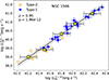 |
Fig. B.1. 0.5–2 keV soft excess luminosity ( |


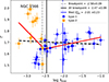 |
Fig. B.2. Relation between the photon index (Γ) and the Eddington ratio (λEdd). The black dashed line represents the linear best fit. The two red lines represent the two-linear fit of the data, with a break. The vertical solid blue and solid black lines represent the median of transition Eddington ratio ( |

Broadband X-ray properties of NGC 1566
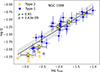 |
Fig. B.3. Variation of soft excess strength (Q) as a function of Eddington ratio (λEdd). The black solid line represents the linear best fit. The gray region marks the 1σ scatter. |
B.2. NGC 2617
NGC 2617 transitioned to type 1 state from type 2 state between 2003 and 2013 (Shappee et al. 2014). Since then, the source remained in type 1 state until 2023. In October 2023, NGC 2617 lost its broad Hβ line and entered a type 2 state (Oknyansky et al. 2023). NGC 2617 showed the presence of soft excess in 2013, when it was in the high-flux state (Giustini et al. 2017). Later the SE emission decreased as it moved toward the type 2 state.
NGC 2617 showed a strong positive correlation between the SE and continuum emission, with a Spearman correlation index of 0.95 with p ≪ 10−10. Figure B.4 shows the variation of the SE emission as a function of continuum emission. The linear fit between the two quantities revealed,  . The observed slope is slightly steeper than that of the whole sample.
In Figure B.5, we show the relation between the Γ and λEdd. The Γ − λEdd relation shows a sharp break at log λEdd = −2.45 ± 0.06, indicating a change of geometry in the inner accretion flow. Figure B.6 displays the relation between the Q and λEdd, which shows strong positive correlations, with ρ = 0.87 and p ≪ 10−10. The observed correlations among different parameters are consistent with the warm Comptonization scenario as the origin of the SE emission. The findings are also consistent with the entire sample.
We found that at log λEdd ∼ −2.5, the SE emission diminishes very rapidly with decreasing accretion rate in NGC 2617. At the same λEdd, the accretion geometry is also found to change. This suggests that the warm corona is closely linked with the inner accretion flow, possibly related to the inner accretion disk. Once the inner accretion disk receded, the warm corona also became weak.
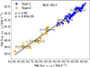 |
Fig. B.4. 0.5–2 keV soft excess luminosity ( |


Broadband X-ray properties of NGC 2617
Broadband X-ray properties of Mrk 590
B.3. Mrk 590
Mrk 590 showed several CS transitions in the past four decades (e.g., Denney et al. 2014; Jana et al. 2025). The source entered a type 2 state in 2006 (Denney et al. 2014), where it remained until 2014. After that, the flux slowly increased, and the source entered a type 1 state in 2017 (Oh et al. 2022). The broadband X-ray properties of Mrk 590 have been studied extensively in the past (e.g., Rivers et al. 2012; Ghosh et al. 2022; Lawther et al. 2023). Mrk 590 showed a variable SE emission, where the SE generally weakens when the primary flux decreases (e.g., Ghosh et al. 2022). Rivers et al. (2012) found that the SE emission decreased by a factor of ∼20 − 30, while the PC emission only changed about ∼10%, suggesting the SE emission is independent of the PC emission. Ghosh et al. (2022) found that SE emission could be explained with both ionized reflection and warm Comptonization scenarios. Palit et al. (2025) reported the emergence of the SE emission when the source transitioned to a type 1 state, when the UV flux also increased. The authors suggested that it is linked with the warm corona, which forms or becomes strong with increasing accretion rate.
Figure B.7 displays the relation between the SE emission and the continuum emission. The SE emission has a strong positive correlation with the continuum emission with ρ = 0.90 and p ≪ 10−10. With linear fitting, we obtained  , with an intrinsic scatter of 0.19 dex (1σ).
We show the relation between the Γ and λEdd in Figure B.8. We obtained a positive correlation between these two parameters. Figure B.9 shows the variation of Q as a function of λEdd. We obtained a positive correlation with ρ = 0.65 and p < 10−5. Broadband spectral analysis revealed the reflection is very weak or absent, suggesting the reflection did not contribute to the SE emission. The correlations we obtained among different parameters indicate that the origin of the SE emission is most probably the warm corona.
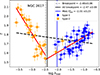 |
Fig. B.5. Relation between the photon index (Γ) and the Eddington ratio (λEdd). The black dashed line represents the linear best fit. The two red lines represent the two-linear fit of the data, with a break. The vertical solid blue and solid black lines represent the median of transition Eddington ratio ( |

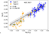 |
Fig. B.6. Variation of soft excess strength (Q) as a function of Eddington ratio (λEdd). The black solid line represents the linear best fit. The gray region marks the 1σ scatter. |
In Mrk 590, we did not observe any change of geometry in the inner accretion flow, although there is a hint of change in slope at log λEdd < −1.5. We also obtained only an upper limit of the SE flux below log λEdd ∼ −2, indicating the warm corona substantially weakens below this.
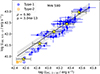 |
Fig. B.7. 0.5–2 keV soft excess luminosity ( |


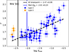 |
Fig. B.8. Relation between the photon index (Γ) and the Eddington ratio (λEdd). The black dashed line represents the linear best fit. The vertical solid blue and solid black lines represent the median of transition Eddington ratio ( |

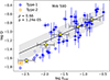 |
Fig. B.9. Variation of soft excess strength (Q) as a function of Eddington ratio (λEdd). The black solid line represents the linear best fit. The gray region marks the 1σ scatter. |
B.4. Mrk 1018
Mrk 1018 is one of the first AGNs that showed CS transitions (Cohen et al. 1986). The source transitioned to type 1 state in 1984, where it remained until 2008 (McElroy et al. 2016). The source moved to type 1.9 state in January 2015 (McElroy et al. 2016). In 2020, the source showed a full CS transition when it briefly entered a type 1 state and moved back to type 1.8 state (Lu et al. 2025).
The broadband X-ray properties of Mrk 1018 have been studied extensively in the past (e.g., Noda & Done 2018; Lyu et al. 2021; Veronese et al. 2024), which agrees with our findings. We find that the reflection is very weak or absent in the broadband X-ray spectroscopy. This agrees with the work of Veronese et al. (2024), who found that no reflection component is needed to model the hard X-ray spectra. We also found evolving SE emission, which is also reported in the previous studies (e.g., Noda & Done 2018). These suggest that warm coronal emission contributes to the SE emission in Mrk 1018.
Figure B.10 displays the relation between the SE and continuum emission of Mrk 1018. Strong positive relation (ρ = 0.89 and p < 10−5.) suggests a common physical origin of the SE and continuum emission. In Figure B.11, we show the relation between Γ and λEdd. We obtained a positive correlation between these two parameters, with a hint of break around log λEdd ∼ −2.5. Figure B.12 shows the variation of Q with λEdd. We obtained ρ = 0.71 and p < 10−5, indicating Q strongly linked with the accretion rate.
In Mrk 1018, we could only probe up to log λEdd ∼ −2.7. Low SE emission indicates that the warm corona becomes weak at this λEdd, and still exists. We expect the warm corona would vanish or diminish at lower λEdd. The observed relations among different parameters are consistent with the warm corona scenario of the SE.
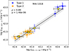 |
Fig. B.10. 0.5–2 keV soft excess luminosity ( |


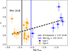 |
Fig. B.11. Relation between the photon index (Γ) and the Eddington ratio (λEdd). The black dashed line represents the linear best fit. The vertical solid blue and solid black lines represent the median of transition Eddington ratio ( |

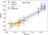 |
Fig. B.12. Variation of soft excess strength (Q) as a function of Eddington ratio (λEdd). The black solid line represents the linear best fit. The gray region marks the 1σ scatter. |
Broadband X-ray properties of Mrk 1018
B.5. IRAS 23226–3843
IRAS 23226–3843 showed several CS transitions in the last decade (e.g., Kollatschny et al. 2020, 2023; Jana et al. 2025). We detected SE emission in the source, which evolves with the accretion rate. Figure B.13 shows the relation of the SE and continuum emission, which shows a strong positive correlation with ρ = 0.95 and p < 10−5. We find the presence of moderate reflection in the source; however, the strength of the Compton hump (reflection strength RS) does not correlate with the Q. This suggests that the SE originates from a warm Corona.
Figure B.14 displays the relation between Γ and λEdd. The Γ − λEdd shows a V-shaped relation with a break at log λEdd ∼ −2.1, indicating a possible change of inner accretion flow. Figure B.15 shows the variation of Q as a function of λEdd. A positive correlation between these two parameters indicates that SE emission is strongly linked with the accretion rate. These relations are consistent with the warm Comptonization scenario as the origin of the SE.
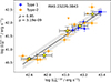 |
Fig. B.13. 0.5–2 keV soft excess luminosity ( |


Broadband X-ray properties of IRAS 23226–3843
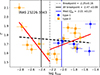 |
Fig. B.14. Relation between the photon index (Γ) and the Eddington ratio (λEdd). The black dashed line represents the linear best fit. The two red lines represent the two-linear fit of the data, with a break. The vertical solid blue and solid black lines represent the median of transition Eddington ratio ( |

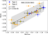 |
Fig. B.15. Variation of soft excess strength (Q) as a function of Eddington ratio (λEdd). The black solid line represents the linear best fit. The gray region marks the 1σ scatter. |
Appendix C: Soft excess model
We modeled SE emission using a phenomenological blackbody (BB) model. We chose this model as we wanted to test both warm corona and ionized reflection scenarios as the origin of the SE. We note that in warm Comptonization scenario, a Comptonization model such as COMPTT or NTHCOMP would provide a more physical description of the SE emission. To test this, we replaced the blackbody component with NTHCOMP and found that the flux in the 0.5–2 keV range remains unchanged. However, when integrating over the broader 0.001–10 keV range, NTHCOMP yields fluxes higher by ∼0.2 dex compared to the blackbody model. This difference does not significantly affect Lbol, as the bulk of the emission originates from the DISKBB and power-law components.
All Tables
Factor of change in the median value of fluxes and soft excess strength between type 1 & type 2 states.
All Figures
|
Fig. 1. Representative unfolded broadband X-ray spectra of NGC 1566 in type 1 and type 2 states (left and right panel, respectively). In the left panel, the orange and blue points represent the data from XMM-Newton/EPIC-PN and NuSTAR/FPMA observations, respectively. In the right panels, the black, orange, and blue points represent the Suzaku/XIS1, Suzaku/XIS0+XIS3, and Suzaku/HXD-PIN observations, respectively. The solid black, dot-dashed black, red dashed, solid magenta, and dotted green lines represent the total, continuum, soft excess, iron K-line, and reprocessed emission, respectively. The middle figures of each panel show the residual, while the data are fitted without the soft excess components. The bottom panels show the residuals for the full models. |
| In the text | |
|
Fig. 2. Light curves of all five CSAGNs in different panels. The blue circles and orange diamonds mark the type 1 and type 2 states, respectively. The vertical lines in each panel represent the optical observations, where the solid blue and orange dot-dashed lines represent the type 1 and type 2 spectral states, respectively. The solid horizontal line in each panel represents the median of transition Eddington ratio |
| In the text | |
|
Fig. 3. Distribution of blackbody temperature (kTBB). The blue dashed and red dot-dashed lines represent the median value for the type 1 and type 2 states, respectively. |
| In the text | |
|
Fig. 4. Variation of the soft excess luminosity ( |
| In the text | |
|
Fig. 5. Relation between Γ and λEdd. The blue circles and orange squares represent the data from the type 1 and type 2 states, respectively. The yellow stars represent the binned data points. The red lines represent the linear best fit of the dataset with a break at log λEdd = −2.47 ± 0.09. The break-point is marked by the vertical gray dashed line. The vertical green dash-dotted line represent the median of the transition Eddington ratio ( |
| In the text | |
|
Fig. 6. Soft excess strength (Q) as a function of Eddington ratio (λEdd). The filled blue circles and orange squares represent the data from type 1 and type 2 states, respectively, while the open blue circles and orange squares represent the upper limits from type 1 and type 2 state, respectively. The yellow stars represent the binned data points, while the yellow down triangle represents the upper limit. The black dashed line represents the best fit. The gray region marks the 1σ scatter. |
| In the text | |
|
Fig. 7. Soft excess strength (Q) as a function of reflection strength (RS). The blue circles and orange squares represent the data from type 1 and type 2 states, respectively. |
| In the text | |
|
Fig. 8. Relation between photon index (Γ) and the soft excess strength (Q) is shown. The blue circles and orange squares represent the data from type 1 and type 2 states, respectively. The open blue circles and orange squares represent the upper limit from type 1 and type 2 states, respectively. The yellow stars represent the binned data points. The black solid lines represent the linear best fit of the dataset with a break at log Q = −1.62 ± 0.12, which corresponds to log λEdd = −2.60 ± 0.14. The break-point is marked by the vertical black dashed line. |
| In the text | |
|
Fig. B.1. 0.5–2 keV soft excess luminosity ( |
| In the text | |
|
Fig. B.2. Relation between the photon index (Γ) and the Eddington ratio (λEdd). The black dashed line represents the linear best fit. The two red lines represent the two-linear fit of the data, with a break. The vertical solid blue and solid black lines represent the median of transition Eddington ratio ( |
| In the text | |
|
Fig. B.3. Variation of soft excess strength (Q) as a function of Eddington ratio (λEdd). The black solid line represents the linear best fit. The gray region marks the 1σ scatter. |
| In the text | |
|
Fig. B.4. 0.5–2 keV soft excess luminosity ( |
| In the text | |
|
Fig. B.5. Relation between the photon index (Γ) and the Eddington ratio (λEdd). The black dashed line represents the linear best fit. The two red lines represent the two-linear fit of the data, with a break. The vertical solid blue and solid black lines represent the median of transition Eddington ratio ( |
| In the text | |
|
Fig. B.6. Variation of soft excess strength (Q) as a function of Eddington ratio (λEdd). The black solid line represents the linear best fit. The gray region marks the 1σ scatter. |
| In the text | |
|
Fig. B.7. 0.5–2 keV soft excess luminosity ( |
| In the text | |
|
Fig. B.8. Relation between the photon index (Γ) and the Eddington ratio (λEdd). The black dashed line represents the linear best fit. The vertical solid blue and solid black lines represent the median of transition Eddington ratio ( |
| In the text | |
|
Fig. B.9. Variation of soft excess strength (Q) as a function of Eddington ratio (λEdd). The black solid line represents the linear best fit. The gray region marks the 1σ scatter. |
| In the text | |
|
Fig. B.10. 0.5–2 keV soft excess luminosity ( |
| In the text | |
|
Fig. B.11. Relation between the photon index (Γ) and the Eddington ratio (λEdd). The black dashed line represents the linear best fit. The vertical solid blue and solid black lines represent the median of transition Eddington ratio ( |
| In the text | |
|
Fig. B.12. Variation of soft excess strength (Q) as a function of Eddington ratio (λEdd). The black solid line represents the linear best fit. The gray region marks the 1σ scatter. |
| In the text | |
|
Fig. B.13. 0.5–2 keV soft excess luminosity ( |
| In the text | |
|
Fig. B.14. Relation between the photon index (Γ) and the Eddington ratio (λEdd). The black dashed line represents the linear best fit. The two red lines represent the two-linear fit of the data, with a break. The vertical solid blue and solid black lines represent the median of transition Eddington ratio ( |
| In the text | |
|
Fig. B.15. Variation of soft excess strength (Q) as a function of Eddington ratio (λEdd). The black solid line represents the linear best fit. The gray region marks the 1σ scatter. |
| In the text | |
Current usage metrics show cumulative count of Article Views (full-text article views including HTML views, PDF and ePub downloads, according to the available data) and Abstracts Views on Vision4Press platform.
Data correspond to usage on the plateform after 2015. The current usage metrics is available 48-96 hours after online publication and is updated daily on week days.
Initial download of the metrics may take a while.