| Issue |
A&A
Volume 707, March 2026
|
|
|---|---|---|
| Article Number | A134 | |
| Number of page(s) | 18 | |
| Section | Planets, planetary systems, and small bodies | |
| DOI | https://doi.org/10.1051/0004-6361/202556700 | |
| Published online | 11 March 2026 | |
Giant Outer Transiting Exoplanet Mass (GOT’EM) survey
VII. TOI-6041: A multi-planet system including a warm Neptune exhibiting strong transit-timing variations
1
Institut d’astrophysique de Paris, CNRS & Sorbonne Université, UMR 7095,
98bis boulevard Arago,
75014
Paris,
France
2
LTE, UMR8255 CNRS, Observatoire de Paris, PSL Univ., Sor-bonne Univ.,
77 av. Denfert-Rochereau,
75014
Paris,
France
3
Center for Space and Habitability, University of Bern,
Gesellschaftsstrasse 6,
3012
Bern,
Switzerland
4
ETH Zurich, Department of Physics,
Wolfgang-Pauli-Strasse 2,
8093
Zurich,
Switzerland
5
Department of Physics and Astronomy, University of New Mexico,
210 Yale Blvd NE,
Albuquerque,
NM
87106,
USA
6
Department of Astronomy and Astrophysics, University of California,
Santa Cruz,
CA
95064,
USA
7
Space Research and Planetary Sciences, Physics Institute, University of Bern,
Gesellschaftsstrasse 6,
3012
Bern,
Switzerland
8
Observatoire astronomique de l’Université de Genève,
Chemin Pegasi 51,
1290
Versoix,
Switzerland
9
Observatoire de Haute-Provence, CNRS, Université d’Aix-Marseille,
04870
Saint-Michel-l’Observatoire,
France
10
European Space Agency (ESA), European Space Research and Technology Centre (ESTEC),
Keplerlaan 1,
2201 AZ
Noordwijk,
The Netherlands
11
Department of Physics, University of Warwick,
Gibbet Hill Road,
Coventry
CV4 7AL,
UK
12
Space Research Institute, Austrian Academy of Sciences,
Schmiedl-strasse 6,
8042
Graz,
Austria
13
Center for Astrophysics |Harvard & Smithsonian,
60 Garden Street,
Cambridge,
MA
02138,
USA
14
CFisUC, Departamento de Física, Universidade de Coimbra,
3004-516
Coimbra,
Portugal
15
Caltech/IPAC-NASA Exoplanet Science Institute,
770 S. Wilson Avenue,
Pasadena,
CA
91106,
USA
16
Dipartimento di Fisica, Università degli Studi di Torino,
via Pietro Giuria 1,
10125
Torino,
Italy
17
Observatoire de Genève, Université de Genève,
51 Chemin Pegasi,
1290
Versoix,
Switzerland
18
NASA Ames Research Center,
Moffett Field,
CA
94035,
USA
19
Amateur Astronomer,
7507 52nd Place NE,
Marysville,
WA
98270,
USA
20
Space sciences, Technologies and Astrophysics Research (STAR) Institute, Université de Liège,
Allée du 6 Août 19C,
4000
Liège,
Belgium
21
Instituto de Astrofisica e Ciencias do Espaco, Universidade do Porto, CAUP,
Rua das Estrelas,
4150-762
Porto,
Portugal
22
Leiden Observatory, University of Leiden,
Einsteinweg 55,
2333 CA
Leiden,
The Netherlands
23
NASA Goddard Space Flight Center,
8800 Greenbelt Rd,
Greenbelt,
MD
20771,
USA
24
Instituto de Astrofísica de Canarias,
Vía Láctea s/n,
38200
La Laguna, Tenerife,
Spain
25
Departamento de Astrofísica, Universidad de La Laguna,
Astrofísico Francisco Sanchez s/n,
38206
La Laguna, Tenerife,
Spain
26
Admatis,
5. Kandó Kálmán Street,
3534
Miskolc,
Hungary
27
Depto. de Astrofísica, Centro de Astrobiología (CSIC-INTA),
ESAC campus,
28692
Villanueva de la Cañada (Madrid),
Spain
28
Departamento de Fisica e Astronomia, Faculdade de Ciencias, Universidade do Porto,
Rua do Campo Alegre,
4169-007
Porto,
Portugal
29
INAF, Osservatorio Astronomico di Padova,
Vicolo dell’Osservatorio 5,
35122
Padova,
Italy
30
Department of Astronomy, Stockholm University, AlbaNova University Center,
10691
Stockholm,
Sweden
31
Institute of Space Research, German Aerospace Center (DLR),
Rutherfordstrasse 2,
12489
Berlin,
Germany
32
Centre for Exoplanet Science, SUPA School of Physics and Astronomy, University of St Andrews,
North Haugh,
St Andrews
KY16 9SS,
UK
33
INAF, Osservatorio Astrofisico di Torino,
Via Osservatorio, 20,
10025
Pino Torinese To,
Italy
34
Centre for Mathematical Sciences, Lund University,
Box 118,
221 00
Lund,
Sweden
35
Aix Marseille Univ, CNRS, CNES, LAM,
38 rue Frédéric Joliot-Curie,
13388
Marseille,
France
36
Univ. Grenoble Alpes, CNRS, IPAG,
38000
Grenoble,
France
37
ARTORG Center for Biomedical Engineering Research, University of Bern,
Bern,
Switzerland
38
ELTE Gothard Astrophysical Observatory,
9700
Szombathely,
Szent Imre h. u. 112,
Hungary
39
SRON Netherlands Institute for Space Research,
Niels Bohrweg 4,
2333 CA
Leiden,
The Netherlands
40
Centre Vie dans l’Univers, Faculté des sciences, Université de Genève,
Quai Ernest-Ansermet 30,
1211
Genève 4,
Switzerland
41
Leiden Observatory, University of Leiden,
PO Box 9513,
2300 RA
Leiden,
The Netherlands
42
Department of Space, Earth and Environment, Chalmers University of Technology,
Onsala Space Observatory,
439 92
Onsala,
Sweden
43
National and Kapodistrian University of Athens, Department of Physics, University Campus,
Zografos
157 84
Athens,
Greece
44
Astrobiology Research Unit, Université de Liège,
Allée du 6 Août 19C,
4000
Liège,
Belgium
45
Department of Astrophysics, University of Vienna,
Türkenschanzstrasse 17,
1180
Vienna,
Austria
46
Institute for Theoretical Physics and Computational Physics, Graz University of Technology,
Petersgasse 16,
8010
Graz,
Austria
47
Department of Earth and Planetary Sciences, University of California,
Riverside,
CA
92521,
USA
48
Vanderbilt University, Department of Physics & Astronomy,
6301 Stevenson Center Ln.,
Nashville,
TN
37235,
USA
49
Konkoly Observatory, Research Centre for Astronomy and Earth Sciences,
1121
Budapest,
Konkoly Thege Miklós út 15–17,
Hungary
50
ELTE Eötvös Loránd University, Institute of Physics,
Pázmány Péter sétány 1/A,
1117
Budapest,
Hungary
51
Institut d’astrophysique de Paris, UMR7095 CNRS, Université Pierre & Marie Curie,
98bis blvd. Arago,
75014
Paris,
France
52
Astrophysics Group, Lennard Jones Building, Keele University,
Staffordshire
ST5 5BG,
UK
53
European Space Agency, ESA – European Space Astronomy Centre,
Camino Bajo del Castillo s/n,
28692
Villanueva de la Cañada,
Madrid,
Spain
54
Institute of Astronomy, Faculty of Physics, Astronomy and Informatics, Nicolaus Copernicus University,
Grudziądzka 5,
87-100
Toruń,
Poland
55
INAF, Osservatorio Astrofisico di Catania,
Via S. Sofia 78,
95123
Catania,
Italy
56
Dipartimento di Fisica e Astronomia “Galileo Galilei”, Università degli Studi di Padova,
Vicolo dell’Osservatorio 3,
35122
Padova,
Italy
57
Cavendish Laboratory,
JJ Thomson Avenue,
Cambridge
CB3 0HE,
UK
58
German Aerospace Center (DLR),
Markgrafenstrasse 37,
10117
Berlin,
Germany
59
Institut fuer Geologische Wissenschaften, Freie Universitaet Berlin,
Malteserstrasse 74-100,
12249
Berlin,
Germany
60
Institut de Ciencies de l’Espai (ICE, CSIC),
Campus UAB, Can Magrans s/n,
08193
Bellaterra,
Spain
61
Institut d’Estudis Espacials de Catalunya (IEEC),
08860
Castelldefels (Barcelona),
Spain
62
Department of Physics and Kavli Institute for Astrophysics and Space Research, Massachusetts Institute of Technology,
Cambridge,
MA
02139,
USA
63
HUN-REN-ELTE Exoplanet Research Group,
Szent Imre h. u. 112.,
Szombathely
9700,
Hungary
64
Institute of Astronomy, University of Cambridge,
Madingley Road,
Cambridge
CB3 0HA,
UK
65
Department of Astrophysical Sciences, Princeton University,
4 Ivy Lane,
Princeton,
NJ
08544,
USA
66
Proto-Logic LLC,
1718 Euclid Street NW,
Washington, DC
20009,
USA
67
SETI Institute, Mountain View, CA 94043 USA/NASA Ames Research Center,
Moffett Field,
CA
94035,
USA
★ Corresponding author: This email address is being protected from spambots. You need JavaScript enabled to view it.
Received:
1
August
2025
Accepted:
27
November
2025
Abstract
We present the characterisation of the TOI-6041 system, a bright (V = 9.84 ± 0.03) G7-type star hosting at least two planets. The inner planet, TOI-6041 b, is a warm Neptune with a radius of 4.55−0.17+0.18 R⊕, initially identified as a single-transit event in TESS photometry. Subsequent observations with TESS and CHEOPS revealed additional transits, enabling the determination of its 26.04945−0.00034+0.00033 orbital period and the detection of significant transit-timing variations (TTVs), exhibiting a peak-to-peak amplitude of about 1 hour. Radial-velocity (RV) measurements obtained with the APF spectrographs allowed us to place a 3σ upper mass limit of 28.9 M⊕ on TOI-6041 b. In addition, the RV data reveal a second companion, TOI-6041 c, on an 88 d orbit, with a minimum mass of 0.25 MJup. A preliminary TTV analysis suggested that the observed variations could be caused by gravitational perturbations from planet c; however, reproducing the observed amplitudes requires a relatively high eccentricity of about 0.3 for that planet. Our dynamical stability analysis indicates that such a configuration is dynamically viable and places a 1σ upper limit on the mass of TOI-6041 c at 0.8 MJup. An alternative is the presence of a third, low-mass planet located between planets b and c, or on an inner orbit relative to planet b – particularly near a mean-motion resonance with planet b – which could account for the observed variations. These findings remain tentative, and further RV and photometric observations are essential in to better constrain the mass of planet b and to refine the TTV modeling, thereby improving our understanding of the system’s dynamical architecture.
Key words: planets and satellites: detection / planets and satellites: dynamical evolution and stability
© The Authors 2026
 Open Access article, published by EDP Sciences, under the terms of the Creative Commons Attribution License (https://creativecommons.org/licenses/by/4.0), which permits unrestricted use, distribution, and reproduction in any medium, provided the original work is properly cited.
This article is published in open access under the Subscribe to Open model. This email address is being protected from spambots. You need JavaScript enabled to view it. to support open access publication.
1 Introduction
Gravitational interactions between planets can induce deviations from strictly periodic transit times – known as transit-timing variations (TTVs; Agol et al. 2005; Holman & Murray 2005). These variations provide a powerful dynamical tool for estimating planetary masses and probing orbital architectures. For instance, TTVs were first used together with radial-velocity (RV) measurements to characterize the Kepler-9 system (Holman et al. 2010) and later enabled the inference of planetary masses from TTVs alone in the Kepler-11 system (Lissauer et al. 2011). In addition, TTVs can be used to confirm planetary candidates or to infer the presence of non-transiting companions, with notable examples including KOI-142 and K2-146 (Nesvornỳ et al. 2013; Hamann et al. 2019).
The NASA Kepler mission, followed by its K2 extension, provided the first large statistical sample of exoplanetary systems with detectable TTVs. This enabled numerous dynamical mass measurements and constraints on mutual inclinations (Holczer et al. 2016; Hadden & Lithwick 2017). While some TTV systems were discovered from the ground (e.g., WASP-148, Hébrard et al. 2020), more recently the NASA TESS mission (Ricker et al. 2015) expanded the catalog of TTV-bearing systems (e.g., Hobson et al. 2023; Heidari et al. 2025). However, its shorter observing windows – typically around 27 d – limit its sensitivity to TTVs, particularly for planets with longer orbital periods (P ≳ 20 d). In a given TESS sector, such planets often appear as single-transit events. The extended mission revisits the same sectors after about two years and occasionally captures a second transit – producing a so-called duotransit. This sparse coverage is usually insufficient for unambiguous period determination or robust TTV detection. Fully characterizing these systems typically requires extensive follow-up, including additional photometric monitoring and RV observations.
In this context, we present the detection and characterization of the TOI-6041 system, a multi-planetary system hosting at least two planets. The inner planet was initially identified as a single-transit event in the TESS data. Subsequent TESS observations, together with our follow-up campaign – including space-based photometry, high-resolution imaging, and RV measurements – have enabled the characterization of both planets in the system and revealed strong TTVs for the inner planet.
The structure of this paper is as follows. In Sect. 2, we present the observational datasets, including TESS and CHEOPS photometry, RV follow-up, and high-resolution imaging. Section 3 describes the stellar characterization. In Sect. 4, we detail the photometric and spectroscopic analysis. The dynamical modeling and TTV analysis are discussed in Sect. 5. Finally, in Sect. 6, we highlight prospects for further follow-up and summarize our conclusions.
2 Observations
2.1 TESS photometry
TESS observed TOI-6041 in three sectors: Sector 18 (November 2019), Sector 58 (November 2022), and Sector 85 (November 2024). A single-transit event was identified in Sector 18 and vetted by the TESS Single Transit Planetary Candidate (TSTPC) group (Harris et al. 2023; Burt et al. 2021) and the Planet Hunters TESS (PHT) citizen scientists (Eisner et al. 2021). After the second transit was detected in Sector 58, the TESS Science Processing Operations Center (SPOC) assigned the system a TESS object of interest (TOI) (Guerrero et al. 2021), as the planetary candidate signal successfully passed all diagnostic tests outlined in the data-validation report (Twicken et al. 2018; Li et al. 2019). These tests included the odd-even transit depth test, the ghost diagnostic test, and the difference-image centroiding test. Based on centroiding analyses from Sectors 18 through 85, the transit signal is located within 1.49 ± 2.53 arcseconds of the host star TOI-6041.
The two transits observed in Sectors 18 and 58 are separated by 1094.06 d. Multiple possible periods are compatible with the detection of the two transits, from the Pmin = 20.260 d (defined from the lack of transits seen in TESS photometry) to Pmax = 1094.06 d (the time interval between the transits). A third transit was later detected in Sector 85, 729 d after the second. It enabled a large number of aliases to be ruled out; however, because it occurred Pmax/3 = 364.7 d after the previous transit, it was insufficient to uniquely determine the period due to the large time gaps and the limited number of observed events in the TESS data alone. Combining the three TESS detections with the non-detections in the light curves therefore leaves a minimum allowed period of 20.260 d and a maximum of 364.7 d.
Nevertheless, such candidates offer a simple avenue for photometric period assessment by targeting the times of transit according to each of the possible periods. This has been performed extensively on long-period targets from the ground (e.g., Schanche et al. 2022; Ulmer-Moll et al. 2022, etc.) and from space (e.g., Osborn et al. 2022; Luque et al. 2023, etc.).
The data analyzed in this paper include two-minute cadence observations processed by the Presearch Data Conditioning–Simple Aperture Photometry (PDC-SAP) pipeline (Stumpe et al. 2012; Stumpe et al. 2014; Smith et al. 2012), provided by the Science Processing Operations Center at NASA Ames Research Center (Jenkins et al. 2016). The TESS light curves were retrieved from the Mikulski Archive for Space Telescopes (MAST1) using the <mono>lightkurve</mono> package (Gaia Collaboration 2018).
We used <mono>tpfplotter</mono> (Aller et al. 2020) to visualize the target pixel files and assess potential light-curve contamination, incorporating sources from Gaia Data Release 3 (DR3; Gaia Collaboration 2016, Gaia Collaboration 2021). Our analysis considered sources within the photometric aperture down to a contrast of six magnitudes. Beyond this threshold, contamination is negligible, contributing less than 0.4%. As shown in Fig. B.1, no stars within the TESS aperture exceed this six-magnitude contrast limit in Sector 18. The same applies to Sectors 58 and 85. We therefore did not include dilution from nearby stars in our joint modeling.
Furthermore, using Eq. (4) from Vanderburg et al. (2019), we estimate that a neighboring star would need to be within a contrast of ∆mag < 2.3 (at 3σ) to be capable of producing the observed transit depth. No such bright stars are present in the TESS aperture, ruling out the possibility that the transit signal is due to a background eclipsing binary. This conclusion is further supported by our high-resolution imaging, which is presented in Sect. 2.6.
2.2 CHEOPS photometry
As discussed in Sect. 2.1, the orbital period of TOI-6041 b remained uncertain based on the TESS data alone. Initial modelling of this TESS data using the <mono>MonoTools</mono> package2 (Osborn 2022) revealed 54 aliases. More usefully, the fit allows the marginal period probability across the aliases thanks to a combination of the transit model likelihood, a geometric transit probability prior, a window function prior (see Kipping 2018), and an eccentricity prior (in this case using a beta distribution derived from populations of planets with 2 < RP < 6 R⊕ from Bern model simulations; Emsenhuber et al. 2021). The result is shown in Fig. C.1. In order to resolve the true period, we turned to observations with CHEOPS.
The CHEOPS mission (Benz et al. 2021; Fortier et al. 2024) is a 30 cm aperture ESA telescope dedicated to the study of transiting exoplanets. It performs high-precision optical photometry in a 330–1100 nm pass band, from a Sun-synchronous and nadir-locked low-Earth orbit. One science case within the CHEOPS GTO has been the determination of the orbital periods of planetary candidates found to have ambiguous periods in TESS photometry (see, e.g., Osborn et al. 2022; Tuson et al. 2023; Psaridi et al. 2024).
TOI-6041 was observed on nine occasions by CHEOPS in 2023 and 2024 (see Table 1). Due to the significant depth of TOI-6041 b and large expected S/N in CHEOPS, we designed an observing strategy in order to flexibly observe partial transits. This allowed for short (three-orbit, ∼5 h) observations to be more easily scheduled between higher priority observations. An initial transit was found at ∼2460254.8 BJD, with the full transit event being observed. This transit occurred exactly Pmax/2 after the second TESS transit, allowing us to exclude half the aliases. A further transit ingress was clearly seen at ∼2460306.9 BJD, which corresponded to two potential periods – either 52.1 or 26.05 d. Finally, in order to determine the period, we observed a time only corresponding to the 26.05 d alias at ∼2460645.5 BJD, finding another clear ingress feature. Together, these three transits determined a period of 26.049 ± 0.001 d for TOI-6041 b.
Due to CHEOPS’ field rotation once per 99 ṁin orbit, substantial detrending is necessary to achieve photometry close to the expected photon noise. We initially processed the sub-arrays using the <mono>PIPE</mono> package3, which models the point spread function (PSF) on the images (see, e.g., Brandeker et al. 2022; Morris et al. 2021). We then used the <mono>chexoplanet</mono> package4 in order to further detrend the CHEOPS photometry. This first assesses which housekeeping data such as background, number of centroids, and on-board temperature correlate with flux, looking at both linear and quadratic trends. It then built a model that decor-relates the flux using these parameters, as well as a spline with ∼9 deg spacing to model rapid changes in flux as a function of spacecraft roll-angle, and a simple transit model (see, e.g., Egger et al. 2024). The result is photometry with a precision of ∼330 ppm/h.
Summary of CHEOPS observations.
2.3 APF spectroscopy
We collected 102 RV measurements of TOI-6041 using the Levy High-Resolution Spectrograph (R ≈ 114 000; Burt et al. 2014) on the 2.4 m Automated Planet Finder (APF) telescope at Lick Observatory (Vogt et al. 2014; Radovan et al. 2014, 2010). Observations were conducted between January 30, 2020, and June 27, 2023. The RVs have a median uncertainty of 2.6 m s−1 and a mean dispersion of 13.2 m s−1. For further details on the instrumental setup and data reduction, see Fulton et al. (2015). Four measurements were excluded due to their high error bars. The complete list of corrected RVs is provided in Table E.1.
2.4 SOPHIE spectroscopy
We observed TOI-6041 using the SOPHIE high-resolution spectrograph mounted on the 193 cm telescope at the Observatoire de Haute-Provence (OHP; Perruchot et al. 2008; Bouchy et al. 2013). SOPHIE has been extensively used to characterize numerous planetary candidates discovered by TESS (e.g., Serrano Bell et al. 2024; Martioli et al. 2023; Heidari et al. 2022; Moutou et al. 2021).
For this study, we obtained four spectra of TOI-6041 between August and October, 2024. The observations were conducted in SOPHIE’s high-resolution mode (R = 75 000) with simultaneous sky monitoring to account for potential contamination from moonlight. Exposure times ranged from 900 to 2100 seconds, depending on weather conditions, and were chosen to achieve a target S/N per pixel of approximately 50 at 550 nm. Two of the spectra had slightly lower S/N values of 45 and 39, but they were still sufficient for our analysis.
The RVs were derived using the standard SOPHIE pipeline, which computes cross-correlation functions (CCFs) as described by Bouchy et al. (2009) and further refined by Heidari et al. (2024). The resulting RV measurements presented in Table E.2 and have typical uncertainties of approximately 2 m/s and a mean dispersion of 11.9 m/s.
2.5 TRES spectroscopy
A reconnaissance spectrum of TOI-6041 was obtained with the Tillinghast Reflector Echelle Spectrograph (TRES; Fűrész 2008), mounted on the 1.5 m Tillinghast Reflector telescope at the Fred Lawrence Whipple Observatory (FLWO) on Mount Hopkins, Arizona. TRES is an optical, fiber-fed echelle spectrograph covering a wavelength range of 390–910 nm with a resolving power of R ≈ 44 000. The TRES spectrum was extracted following the procedure described by Buchhave et al. (2010). This spectrum was only used for our stellar classification presented in Sect. 3.
2.6 High-resolution imaging
As a usual part of the validation and confirmation process for transiting exoplanets, high-resolution imaging is one of the critical assets required. The presence of a close companion star, whether truly bound or in the line of sight, will provide “third-light” contamination of the observed transit, leading to derived properties for the exoplanet and host star that are incorrect (Ciardi et al. 2015; Furlan & Howell 2017, 2020; Bouma et al. 2018). In addition, it has been shown that the presence of a close companion dilutes small planet transits (<1.2 Re) to the point of non-detection (Lester et al. 2021). Given that nearly half of FGK stars are in binary or multiple-star systems (Matson et al. 2018), high-resolution imaging provides crucial information toward our understanding of each discovered exoplanet as well as more global information on exoplanetary formation, dynamics, and evolution (Howell et al. 2021).
TOI-6041 was observed on 2020 December 02 and 2021 February 03 using the ‘Alopeke speckle instrument on the Gemini North 8-m telescope (Scott et al. 2021). ‘Alopeke provides simultaneous speckle imaging in two bands (562 nm and 832 nm) with output final data products including a reconstructed image with robust contrast limits on companion detections (e.g., Howell et al. 2016). While both observations had consistent results showing that TOI-6041 is a single star, within the achieved angular resolution and 5σ magnitude contrast limits, the December 2020 observation had better seeing, which led to deeper contrast levels in the 562 nm band. Four sets of 1000 × 0.06 second images were obtained and processed in our standard reduction pipeline (see Howell et al. 2011). Figure D.1 shows our final contrast curves and the 562 nm and 832 nm reconstructed speckle images. We find that TOI-6041 is a single star with no companion brighter than five-to-nine orders of magnitude below that of the target star from the 8-m telescope diffraction limit (20 mas) out to 1.2”. At the distance of TOI-6041 (d=72 pc), these angular limits correspond to spatial limits of 1.44–86.4 AU.
3 Stellar characterization
To determine the stellar atmospheric parameters, we first combined the SOPHIE spectra of TOI-6041 to construct a high S/N template, after correcting for both the star’s RV variation and the barycentric Earth RV. We then applied the methodology of Sousa et al. (2011), Santos et al. (2013), and Sousa et al. (2018) to derive the effective temperature (Teff), metallicity ([Fe/H]), and surface gravity (log g). A more accurate trigonometric log g was also derived using Gaia DR3 data, following the procedure described in Sousa et al. (2021). Additionally, we estimated the projected stellar rotational velocity (vsin i) for each individual SOPHIE spectrum using the calibration of Boisse et al. (2010) and then computed the mean value, which we report in Table 2 along with other stellar properties.
As an independent analysis, we also derived stellar parameters from the TRES spectrum using the Stellar Parameter Classification (SPC; Buchhave et al. 2012) tool. The SPC cross-correlates the observed spectrum with a grid of synthetic spectra based on Kurucz atmospheric models (Kurucz 1992) to determine the star’s Teff, [Fe/H], log g, and vsin i. Following the recommendation of Tayar et al. (2022), we conservatively adopted a systematic uncertainty floor on the TRES-derived Teff, which can be seen in brackets in Table 2. For the SOPHIE-derived Teff, the systematic uncertainty had already been included in the reported uncertainty (Sousa et al. 2011). The stellar parameters derived from the TRES spectrum are consistent within 1σ with those obtained from the SOPHIE spectra, as summarized in Table 2.
An analysis of the broadband spectral energy distribution (SED) of the star was performed together with the Gaia DR3 parallax, in order to determine an empirical measurement of the stellar radius (Stassun & Torres 2016; Stassun et al. 2017, 2018). The JHKS magnitudes were sourced from 2MASS (Skrutskie et al. 2006), the W1–W4 magnitudes from WISE (Wright et al. 2010), the GBPGRP magnitudes from Gaia (Gaia Collaboration 2023), and the NUV magnitude from GALEX (Martin et al. 2005). The absolute flux-calibrated Gaia spectrum was also utilized, when available. Together, the available photometry spans the full stellar SED over the wavelength range of at least 0.4–10 µm and at most 0.2–20 µm (see Fig. 1).
A fit using PHOENIX stellar atmosphere models (Husser et al. 2013) was performed, adopting the Teff, [Fe/H], and log g from the SOPHIE spectroscopic analysis. The extinction, AV, was fit for, limited to the maximum line-of-sight value from the Galactic dust maps of Schlegel et al. (1998). The resulting fit (Fig. 1) has an χ2 = 16.2, excluding the GALEX NUV flux, which indicates a moderate level of activity (Findeisen et al. 2011), with the best-fit AV = 0.03 ± 0.03. Integrating the (unreddened) model SED gives the bolometric flux at Earth, Fbol = 3.233 ± 0.075 × 10⁻⁹ erg s−1 cm−2. Taking the Fbol together with the Gaia parallax directly gives the bolometric luminosity, Lbol = 0.532 ± 0.012 L⊙. The Stefan-Boltzmann relation then gives the stellar radius, R⋆ = 0.855 ± 0.023 R⊙. In addition, the stellar mass was estimated using the empirical relations of Torres et al. (2010), with the offset correction applied following Santos et al. (2013), yielding M⋆ = 0.85 ± 0.01 M⊙. We note that the intrinsic error from the Torres et al. (2010) calibration was also added in quadrature to the final uncertainty.
The formal error estimates for the stellar radius from our SED analysis may be underestimated. For a star such as TOI-6041, the systematic uncertainty floor is expected to be approximately 4.2% in radius, as suggested by Tayar et al. (2022). To account for this, we conservatively adopted these relative uncertainties and report them in brackets in Table 2. In the case of the stellar mass, our uncertainty is consistent with this systematic uncertainty floor.
We estimated the stellar rotation period using the method described in Suárez Mascareño et al. (2016), which relies on the activity–rotation relation calibrated for different spectral types using the chromospheric activity index log ( ). For this G-type star, we applied the corresponding calibration with log (
 ) = −4.7 ± 0.1, derived from the SOPHIE spectra following the procedures of Noyes et al. (1984) and Boisse et al. (2010). We compare this with the value obtained from Mamajek & Hillenbrand (2008), which incorporates both log(
 ) and the B − V color. These methods yield rotation periods of 23 ± 5 days and 29 ± 5 days, respectively, consistent within approximately 1σ.
To further investigate the stellar rotation period, we applied the Lomb-Scargle periodogram to the SAP TESS light curves from all three available sectors, with periods from 0 to 50 d. We detected a strong, broad peak between approximately 20 and 30 d, with a false alarm probability below 0.001% (see the periodogram and phase-folded light curve in Fig. F.1). This signal is consistent with the rotation periods estimated from log( ) and is likely associated with rotational modulation. Its broad nature may be attributed to the limited time baseline of each TESS sector, which spans only about 27 d. Additionally, using the empirical age–activity relations of Mamajek & Hillenbrand (2008), we estimate an age of 2.0 ± 1.1 Gyr.
Finally, as a further check, we compared these values with results obtained using an alternative modeling method in <mono>EXOFASTv2</mono>, performed simultaneously with the planetary fit (see Sect. 4.2). The parameters agree within 1σ, except for the stellar age, which is only consistent at the 2σ level. However, we note that the stellar age derived from the <mono>EXOFASTv2</mono> fit is poorly constrained, yielding a broad and asymmetric posterior distribution (see Fig. G.1).
Stellar properties of TOI-6041.
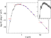 |
Fig. 1 Spectral energy distribution of TOI-6041. Red symbols represent the observed photometric measurements, where the horizontal bars represent the effective width of the pass band. Blue symbols show the model fluxes from the best-fit PHOENIX atmosphere model (black). The absolute flux-calibrated Gaia spectrum is shown as a gray swathe in the inset figure. |
4 Detection and characterization of TOI-6041’s planets
4.1 RV-only analysis
We began our RV analysis by performing a periodogram analysis of the RVs and the S-index activity indicator using the Data and Analysis Center for Exoplanets (DACE; Delisle et al. 2016)5. Since we only had four SOPHIE RV measurements, we only used the APF data in this section to avoid instrumental offsets between the two datasets, while we also tested fits including both datasets in our global modeling in Sect. 4.2.
The periodogram of RVs showed a significant peak at 88 d, below the analytical false alarm probability (FAP, Baluev 2008) of 0.1% (see Fig. 2, first panel). We modelled and subtracted this signal using a circular Keplerian fit (see justification below). The periodogram of the residuals then reveals a peak at 0.9 d and a tentative signal around 11 d, both with FAP values close to 10% (see Fig. 2, second panel). These two signals are aliases of each other and are not statistically significant. Additional RV measurements are required to understand their origin. Finally, we detect neither a significant signal in the S-index activity periodogram (see Fig. 2, third panel) nor any correlation between the S-index and the RVs (Pearson’s correlation coefficient r =−0.1) or their residuals (r=0.3) after removing the 88 d signal.
Additionally, we considered several RV-only models and performed model comparisons. The RV analysis was conducted using <mono>juliet</mono> (Espinoza et al. 2019), which employs RadVel (Fulton et al. 2018) to model the RVs. Since we found no significant influence of stellar activity in our RVs, we did not include a Gaussian process in our analysis. For each tested model, <mono>juliet</mono> computes the Bayesian log evidence (ln Z). A model is considered moderately favored over another if the difference in Bayesian log evidence (∆ ln Z) exceeds two, while a difference greater than five indicates strong preference (Trotta 2008). When ∆ ln Z ≤ 2, the models are statistically indistinguishable, and in such cases, the model with the fewest free parameters is preferred.
First, we tested a no-planet model (No-planet) and a one-Keplerian model with circular orbit and a uniform prior on the orbital period between 70 and 100 d (1cpl). For the remaining parameters, we adopted fairly broad uniform priors. The one-Keplerian model converged on the 88 d signal. As shown in Table 3, the ∆ ln Z between these two models is 25.0, indicating a strong detection of the 88 d signal. We then considered a one-Keplerian model with a freely varying eccentricity (1cpl), which yielded a best-fit eccentricity of e = 0.3 ± 0.2. However, since the eccentricity is not significantly detected and the ∆ ln Z values for the circular and eccentric models are indistinguishable, we adopted the circular model for our final analysis.
Next, we tested a two-Keplerian model on 88 d and 26 d signals (2cpl). Since we did not observe a signature for the 26 d periodic signal in the RV periodogram, we fixed the transit epoch (T0) and period to the values derived from photometry for this planet (see Sect. 2.2) and ran the model. This model converged with an amplitude of  for this signal, but it reached the prior edge. The ∆ ln Z comparison showed this model is indistinguishable from the one-Keplerian model, indicating no significant detection of 26 d signal in RVs, which is consistent with the results of the periodogram.
Finally, we tested a three-Keplerian model with an additional planet candidate with a circular orbit and a uniform prior on the period ranging from 0 to 20 d (3cpl). This model was motivated by the tentative 0.9 d and 11 d signals observed in the residual periodogram. The fit converged on an 11 d signal. However, this model remained statistically indistinguishable from the one-planet model, confirming that the 11 d signal is not statistically significantly detected.
Therefore, we conclude that the only robustly detected signal in our RV data is the 88 d signal. Since this signal has no corresponding signal in the S-index activity indicator, it is likely of planetary origin. In the rest of this paper, we refer to it as TOI-6041 c.
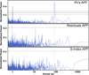 |
Fig. 2 Periodograms of RV and S-index derived from APF data for TOI-6041. From top to bottom: APF RVs, residuals of the RVs after a Keplerian fit to the 88 d signal, and the S-index activity indicator. The vertical pink line marks the planet candidate with a period of 88 d, which shows no corresponding signal in the S-index periodogram. The horizontal lines indicate false alarm probability (FAP; Baluev 2008) thresholds of 0.1%, 1%, and 10%, respectively, from top to bottom. |
Comparison of different models tested using RV-only data analyzed with <mono>juliet</mono>.
4.2 Global modeling
To simultaneously model the stellar and planetary parameters, we used <mono>EXOFASTv2</mono> (Eastman et al. 2013; Eastman 2017; Eastman et al. 2019). Our analysis incorporated photometric data from three TESS sectors, three CHEOPS observations, and RVs from APF. We applied Gaussian priors on [Fe/H], centered on the value derived from the SOPHIE spectrum (Sect. 3), but adopted a conservatively broad standard deviation equal to twice its reported uncertainty. A Gaussian prior was also applied to the parallax, using values from the Gaia DR3 catalog. Additionally, we imposed an upper limit on extinction, AV, based on the dust maps from Schlegel et al. (1998). The broadband photometry, as presented in Table 2, is also included. The Gaia DR3 parallax, the AV upper limit, and the broadband photometry were used to constrain the stellar properties through SED fitting. To compare our results, we also modeled the star using the MESA Isochrones and Stellar Tracks (MIST; Dotter 2016; Choi et al. 2016) method. As part of the modeling process, we simultaneously detrended the TESS photometry using a spline (Vanderburg & Johnson 2014) within <mono>EXOFASTv2</mono> to mitigate instrumental systematics (see Sect. 2.2 for the CHEOPS detrending procedure). We did not impose any priors on the planetary parameters, allowing <mono>EXOFASTv2</mono> to explore them freely (see Eastman et al. (2013), Eastman (2017), and Eastman et al. (2019) for detailed information).
We began our analysis with a circular orbit model for both planets. Upon convergence, we observed a significant TTV signal for TOI-6041 b (see Fig. H.2). To account for this, we incorporated a TTV model using <mono>EXOFASTv2</mono> as part of our joint analysis and re-ran the fit. We note that the TTVs in this model correspond to artificial shifts added to a Keplerian model, which allows for a first estimate of the system parameters. In most cases, such an approach provides suitable parameter estimates (see, e.g., Hébrard et al. 2020; Almenara et al. 2022). Mutual gravitational interactions are taken into account below in Sect. 5. The updated model, which included TTVs, was strongly favored by the Bayesian information criterion (BIC), with a difference of ∆BIC = 543.8 compared to the Keplerian-only model. This indicates a significantly better fit to the data. We chose this model as the final one and present the posterior distributions of all model parameters in Table 4 and Table I.1, while the best-fit model for both the RV and photometric data is shown in Fig. 3.
Including TTVs in the model allowed the transit times to deviate from those predicted by a purely Keplerian orbit and a strictly linear ephemeris. <mono>EXOFASTv2</mono> determined the mid-transit times based on both a linear ephemeris and a TTV model, and provide the corresponding observed-minus-calculated (O–C) diagram (see Fig. H.1). A summary of the observed mid-transit time and the TTV measurements is provided in Table 5 (see Sect. 5 for a more detailed discussion of the system’s TTVs). The TTVs display a peak-to-peak variation of 57.2 minutes and an RMS scatter of 28 minutes.
We also tested fits that included the SOPHIE RVs. However, given that only four SOPHIE measurements were available, the corresponding RV jitter term could not be robustly constrained. Importantly, including or excluding these four data points did not affect our results. We therefore chose not to include the SOPHIE RVs in our final analysis. The results indicate that TOI-6041 has a mass of  , a radius of 0.879 ± 0.026 R⊙, and an effective temperature of
  . These values are consistent within 1σ with those derived from the spectral analysis and SED fitting presented in Sect. 3, with the exception of the stellar age, which differs at the 2σ level. However, we note that the age estimate from the <mono>EXOFASTv2</mono> analysis remains weakly constrained, yielding a broad and skewed posterior distribution (see Fig.G.1).
For TOI-6041 b, accounting for the observed TTV signal, we determine an average orbital period of  d and a radius of
  . Although this planet is not unambiguously detected in our RV data, the measurements allow us to place a 3σ upper limit on its RV semi-amplitude of 7 m s−1, corresponding to a maximum mass of 28.9 M⊕. Additional RV observations are needed to more tightly constrain the mass of TOI-6041 b.
We also tested a model allowing a nonzero eccentricity for TOI-6041 b. However, the MCMC chains did not converge well due to a strong bimodality in the argument of periastron (ω), with two dominant modes around 20◦ and 230◦. The posterior distribution of the eccentricity spans the entire prior range (0–1), with 68% of the probability lying below 0.6. We therefore conclude that the current data do not support a significant eccentricity detection for TOI-6041 b. As before, additional observations – both RV and TTV – are needed to better constrain the planet’s eccentricity.
The outer planet, TOI-6041 c, is detected solely through our RV measurements. It has an orbital period of  d and a minimum mass of
  . We adopted a circular orbit for this planet, as the eccentricity is not significantly constrained by the data (see Sect. 4.1). We also note that including or excluding an RV model for TOI-6041 b does not affect the derived parameters of TOI-6041 c. Whether TOI-6041 c is transiting remains uncertain, as the time of periastron listed in Table 4 has an uncertainty of approximately 12 d. Each TESS sector provides about 27 d of coverage, and a data gap occurs about near the midpoint of the relevant sector. It is therefore possible that a potential transit fell within this gap. Additional RV measurements are required to better constrain the time of periastron and to assess the planet’s transit probability.
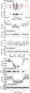 |
Fig. 3 APF RV measurements of TOI-6041 (top panel); phase-folded RVs for TOI-6041c (second panel) and TOI-6041b (third panel); and the phase-folded CHEOPS and TESS light curves for TOI-6041b (fourth and fifth panels). The red lines show the best-fit models derived using EXOFASTv2. Residuals are displayed at the bottom of each panel. |
5 Dynamical analysis
In this section we present a dynamical analysis of the TOI-6041 system to assess the long-term stability of its orbital configuration and to investigate whether the observed TTVs of planet b can be explained by its gravitational interactions with the outer planet c. Although several transits of planet b have been observed, the planet is not detected in RVs; planet c, conversely, is detected via RVs but does not transit. This limits our ability to constrain the system’s orbital architecture. The analysis presented here should therefore be regarded as exploratory, pending additional observational constraints. Additional data would benefit from a photodynamical analysis (see, e.g., Almenara et al. 2022).
Median values and 68% confidence intervals for TOI-6041 and its two planets.
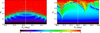 |
Fig. 4 Stability analysis of TOI-6041 system. The phase space of the system is explored by varying the orbital period, Pi, and eccentricity, ei, of each planet independently. For each initial condition (Table 4), the system is integrated over 10 kyr, and a stability criterion is derived with the frequency analysis of the mean longitude. The chaotic diffusion is measured by the variation in the frequencies. The color-scale corresponds to the logarithmic variation in the stability index used in Correia et al. (2010). The red zone corresponds to highly unstable orbits, while the dark blue region can be assumed to be stable on a billion-year timescale. Dashed white lines indicate the nominal orbital periods reported in Table 4. |
Median values and 68% confidence interval for transit times, and TTVs.
5.1 Stability analysis
We first performed a global frequency analysis (Laskar 1990, 1993) in the vicinity of the best fitting circular solution (Table 4), using the methodology described in Correia et al. (2005), Correia et al. (2010), and Couetdic et al. (2010). The goal is to assess the long-term stability of the orbital solution. The system was integrated on a regular 2D mesh of initial conditions, varying the orbital period and eccentricity of each planet individually, while keeping all other orbital elements fixed to the values listed in Table 4. The integrations were carried out using the symplectic integrator SABA1064 of Farrés et al. (2013), with a time step of 5 × 10⁻³ yr, and included general-relativity corrections. Each initial condition was integrated over 10 kyr, and a stability indicator was derived with the frequency analysis of the mean longitude, to be the variation in the measured mean motion over the two consecutive 5 kyr intervals of time (for more details, see Couetdic et al. 2010). For regular motion, there is no significant variation in the mean motion along the trajectory, while it can vary significantly for chaotic trajectories. The results are shown in Fig. 4, where “red” represents the strongly chaotic trajectories, and “dark blue” denotes extremely stable regions. We observe that the system remains stable for eccentricities up to ∼0.15 for planet b and ∼0.3 for planet c.
Additionally, we computed a 2D stability map for the two unconstrained orbital parameters of planet c – the inclination, ic, and the longitude of the ascending node, Ωc – to assess how dynamical arguments can constrain their possible values. Figure 6 explores the stability in the (Ωc, ic) plane, with all other orbital elements fixed to the values listed in Table 4. We find that the system remains stable for 20◦ ≲ ic ≲ 160◦, corresponding to mutual inclinations up to about 70◦. This dynamical constraint allows us to place an upper limit on the true mass of planet c, despite the absence of a transit. Given the 1σ upper bound on the minimum mass, mc sin ic < 0.274MJup, and the inclination, ic ≲ 160◦, we infer a 1σ upper limit on the true mass of mc ≲ 0.80MJup.
5.2 Transit-timing variations
To investigate the origin of the observed TTVs in planet b, we generated synthetic TTV signals using <mono>TTVFast</mono> (Deck et al. 2014) for different orbital configurations of planet c. Adopting the circular and coplanar setup from Table 4, we found that the resulting TTV amplitudes remained below 2 minutes; these are significantly smaller than the observed variations. Reducing the inclination of planet c (and thereby increasing its true mass) increased the amplitude somewhat, but it remained insufficient to match observations.
In contrast, increasing the eccentricity of planet c had a stronger effect on the TTVs: for ec ∼ 0.3 (i.e., the largest stable value; see Sect. 5.1), the simulated TTV amplitudes become comparable to those observed. However, the shape of the signal becomes highly sensitive to the initial orbital phase angles, particularly the argument of pericenter ωc and mean longitude λc. Figure 5 illustrates this degeneracy by showing two configurations with identical eccentricity but different ωc values. This highlights a key limitation of TTV modeling: different combinations of poorly constrained orbital elements can yield similar TTV signatures (Lithwick et al. 2012). It is worth noting that the period ratio between planets b and c is close to a 7:2 commensurability, corresponding to a fifth-order mean-motion resonance (MMR). Such a high-order resonance would typically generate weaker TTV signals unless the perturber has a relatively large eccentricity, consistent with the value required in our modeling. Moreover, in observed systems, TTVs are often associated with first- or second-order MMRs, which makes it less likely that planet c alone is responsible for the observed TTVs for planet b. Additional photometric observations will be needed to improve the analysis of the TTVs and assess the viability of this configuration.
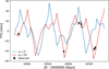 |
Fig. 5 Transit-timing variations of TOI-6041b planet. We adopted ec = 0.3 and two values of the argument of pericenter: ωc = 0◦ (blue) and ωc = 50◦ (red). All other parameters are fixed at their nominal values from Table 4. The dots correspond to the observed TTVs. While the amplitudes are consistent with observations, the signal shape depends strongly on the orbital phase angles. |
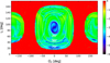 |
Fig. 6 Stability analysis of TOI-6041 system in the (Ωc, ic) plane. The phase space is explored by varying these two parameters, while all other orbital elements are fixed to the nominal values in Table 4. As in Fig. 4, red regions indicate strongly chaotic orbits, while dark blue regions correspond to long-term stability. White curves denote levels of constant mutual inclination between planets b and c. |
5.3 Effect of a potential third planet
A tentative 11 d signal in our RV-only analysis presented in Sect. 4.1, suggests the possible presence of an additional inner planet. To evaluate its potential dynamical impact, we included a hypothetical third planet in our numerical simulations. We assumed a circular orbit with P = 11 d, a RV semi-amplitude of K = 0.5 m/s, and all orbital angles set to 0◦, except for the inclination (i = 90◦). We first verified that the system remains dynamically stable in the presence of this third planet. To investigate this, we varied its semi-major axis and eccentricity over a wide range and performed a stability analysis. The stability map (Fig. J.2) reveals that stable orbits are indeed possible for semi-major axes below 0.15 AU, corresponding to orbital periods shorter than 22 d.
Next, we tested its impact on the TTVs of planet b. In the circular and coplanar configuration for all three planets, the additional planet’s influence is negligible: the resulting TTVs remain below 2 minutes. Its effect remained negligible across the different orbital configurations we explored. For example, in Fig. 7, we adopt the favorable setup previously shown to reproduce the observed TTVs – specifically ec = 0.3 and ωc = 50◦ for planet c – and include the additional planet while varying its eccentricity, e, between 0 and 0.4. The resulting TTV signal of planet b remains essentially unchanged.
We further tested several near-resonant periods for this additional inner planet, placing it closer to low-order MMRs with planet b (e.g., 3:2, 4:3, and 5:4). Such resonances could enhance the gravitational interactions with planet b and potentially account for the large observed TTV amplitudes. Specifically, we ran numerical simulations with the third planet placed at orbital periods of 17.3, 19.63, and 20.96 d, and computed the TTVs of planet b, assuming circular and coplanar orbits for all three planets. As shown in Fig. J.1, the resulting TTV amplitudes can be comparable to those observed, particularly for the periods near the 4:3 and 5:4 MMRs. In this configuration, the additional planet acts as the main perturber inducing TTVs on planet b, while planet c contributes negligibly. The exact shape of the signal remains sensitive to the poorly constrained orbital elements and the inherent degeneracies of TTV modeling. Nevertheless, this provides a plausible explanation for the observed TTVs of planet b that does not require a high eccentricity for planet c.
We also explored the possibility of a third undetected planet located between planets b and c, assuming the same RV semi-amplitude (K = 0.5 m/s) as before. As shown in Fig. J.2, stable orbits exist in this region for low eccentricities, particularly near 0.25 AU, corresponding to orbital periods between approximately 30 and 70 d. This range includes several possible MMRs; for instance, a planet with a period of around 34.7 d lies near the 4:3 MMR with planet b and the 5:2 MMR with planet c, whereas a period of around 39 d corresponds to the 3:2 MMR with planet b and the 9:4 MMR with planet c.
To test its impact on the TTVs of planet b, we placed the third planet at orbital periods of 36 and 41 d and computed the TTVs of planet b, again assuming circular and coplanar orbits for all three planets. As shown in Fig. J.3, these configurations also produce TTV amplitudes of the same order as the observed variations. In this case, the additional planet acts as the main perturber inducing TTVs on planet b, though planet c also contributes non-negligibly to the signal. As before, the detailed signal shape remains sensitive to the poorly constrained orbital elements and the inherent degeneracies of TTV modeling. Nevertheless, this scenario offers another plausible explanation for the observed variations. It does not require a high eccentricity for planet c and is consistent with the expectation that the dynamically stable region between planets b and c could host an additional, undetected planet. New transit observations and RV measurements will be essential to confirm the presence of such possible companions and to refine the TTV modeling.
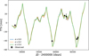 |
Fig. 7 Transit-timing variations of TOI-6041b in a three-planet model including the hypothetical 11 d planet. We adopted the same favorable configuration as in Fig. 5, with ec = 0.3 and ωc = 50◦, and varied the eccentricity of the additional planet, e, from 0 to 0.4. The resulting curves show negligible differences, confirming that planet c likely is the dominant source of the observed TTVs in this configuration. |
6 Summary and discussion
TOI-6041 is a G7-type star with a radius of R∗ = 0.879 ± 0.026 R⊙ and a mass of  , and it is located at a distance of 72.3 ± 0.1 pc. The system hosts at least two planets. The inner planet, TOI-6041 b, is a transiting Neptune-like planet with a period of
  d, a radius of
  , and a 3σ upper limit on the RV semi-amplitude of 7 m s−1, corresponding to a maximum mass of 28.9 M⊕. This constraint implies a bulk density below approximately 1.7 g cm−3, suggesting the presence of a substantial gaseous envelope. Further RV measurements would enhance the precision of the inner planet’s mass estimate and enable modeling of its internal structure.
The outer companion, TOI-6041 c, is detected only through our RV measurements and has a minimum mass of  MJup and an orbital period of
  d. Preliminary dynamical modeling of the observed TTVs of TOI-6041 b suggests that they could arise from gravitational perturbations by planet c, although matching the observed amplitudes requires a relatively high eccentricity of about 0.3. By integrating the dynamical stability analysis with the observed minimum mass constraints, we derive a 1σ upper bound on the true mass of planet c of approximately 0.80 MJup. An alternative is the presence of a third, low-mass planet located between planets b and c or on an inner orbit relative to planet b – particularly near an MMR with planet b – which could significantly contribute to the observed variations. In this three-planet configuration, the observed TTV amplitudes can be reproduced without requiring large eccentricities.
With a magnitude of V = 9.84 ± 0.03 mag, TOI-6041 is a good candidate for follow-up observations. Using the 3σ upper-mass limit of the inner planet, we estimate a lower bound on the transmission spectroscopy metric (TSM; Kempton et al. 2018) of TSM ≥ 59, suggesting that TOI-6041 b is a good target for atmospheric characterization. This is particularly compelling given its estimated equilibrium temperature of  , which places the planet near the so-called “hazy-atmosphere” regime (270– 600 K) proposed by Yu et al. (2021). This offers an opportunity to probe haze formation and to characterize atmospheric compositions above it (Kawashima et al. 2019). Moreover, cooler atmospheres may exhibit disequilibrium chemistry, providing additional insight into atmospheric processes and their underlying physics (Fortney et al. 2020).
In parallel, TOI-6041 b is well suited for spin–orbit alignment measurements, which can help constrain its dynamical history. Using Eq. (6) of Gaudi & Winn (2007), we estimated a Rossiter–McLaughlin (RM; McLaughlin 1924; Rossiter 1924) semi-amplitude of 7.7 ± 2.4 m s−1, which is within reach of high-precision spectrographs such as HARPS-N. Moreover, the relatively high-impact parameter of the transit (b= 0.74 ± 0.02) is advantageous for RM observations, as it reduces the degeneracy between v sin i⋆ and the projected spin–orbit angle λ (see Gaudi & Winn 2007), thereby allowing for a more precise determination of λ. Planets on relatively long-period orbits, such as TOI-6041 b, are particularly valuable for RM observations, as their spin–orbit angles are less likely to have been modified by tidal realignment (Li & Winn 2016), and therefore they may retain signatures of their formation and migration histories.
The location of TOI-6041 b in the so-called Neptunian “savanna” further strengthens the scientific interest of this system (see Fig. 8). This region of parameter space corresponds to a milder deficit of intermediate-sized planets at longer orbital periods and lower levels of stellar irradiation (Bourrier et al. 2023), in contrast to the more pronounced Neptunian desert at shorter periods (P ≲ 4 d; Mazeh et al. 2016). While the origin of these features in the radius–period plane is not fully understood, several physical mechanisms have been proposed.
Runaway gas accretion, which is predicted to occur beyond the ice line, is one such mechanism thought to contribute to the gap between sub-Neptunes and gas giants (Pollack et al. 1996; Lissauer et al. 2009). The presence of TOI-6041 b and other similar planets, located well within the ice line, therefore raises the question of whether it formed in situ or instead migrated inward after formation. If migration occurred, the nature of the process–whether through smooth disk-driven migration or high-eccentricity dynamical interactions–could leave observable signatures, such as spin–orbit misalignments or nonzero orbital eccentricities. Continued characterization of the system, including improved mass constraints, eccentricity measurements, and RM observations, could thus provide valuable information on the migration pathways of Neptunian planets in this transitional regime.
Finally, the significant TTVs observed in this system offer a valuable opportunity to study planet–planet gravitational interactions. Additional photometric and RV observations will also be essential to refine the TTV analysis and to better characterize the architecture and interactions within the system.
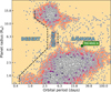 |
Fig. 8 Location of TOI-6041 b within radius–period diagram, along with other known exoplanets whose radius precision is better than 30%, taken from the NASA Exoplanet Archive (https://exoplanetarchive.ipac.caltech.edu/) as of June 5, 2025. The background-density map illustrates the distribution of confirmed exo-planets, with regions labeled as the desert, ridge, and savanna to reflect differing planet-occurrence rates (Castro-González et al. 2024). TOI-6041 b (green marker) lies in the savanna region. This plot was generated using the <mono>nep-des</mono> Python code (https://github.com/castro-gzlz/nep-des). |
Acknowledgements
N.H. acknowledges support from a postdoctoral fellowship funded by the Domaine de Recherche et d’Innovation Majeur (DIM), financed by the Île-de-France Region. This work was granted access to the HPC resources of MesoPSL financed by the Region Île-de-France and the project Equip@Meso (reference ANR-10-EQPX-29-01) of the programme Investissements d’Avenir supervised by the Agence Nationale pour la Recherche. We warmly thank the OHP staff for their support on the observations. We received funding from the French Programme National de Physique Stellaire (PNPS) and the Programme National de Planétologie (PNP) of CNRS (INSU). This paper made use of data collected by the TESS mission which is publicly available from the Mikulski Archive for Space Telescopes (MAST) operated by the Space Telescope Science Institute (STScI). Funding for the TESS mission is provided by NASA’s Science Mission Directorate. We acknowledge the use of public TESS data from pipelines at the TESS Science Office and at the TESS Science Processing Operations Center. Resources supporting this work were provided by the NASA High-End Computing (HEC) Program through the NASA Advanced Supercomputing (NAS) Division at Ames Research Center for the production of the SPOC data products. Some of the observations in this paper made use of the High-Resolution Imaging instrument ‘Alopeke and were obtained under Gemini LLP Proposal Number: GN/S-2021A-LP-105. ‘Alopeke was funded by the NASA Exoplanet Exploration Program and built at the NASA Ames Research Center by Steve B. Howell, Nic Scott, Elliott P. Horch, and Emmett Quigley. Alopeke was mounted on the Gemini North telescope of the international Gemini Observatory, a program of NSF’s OIR Lab, which is managed by the Association of Universities for Research in Astronomy (AURA) under a cooperative agreement with the National Science Foundation. on behalf of the Gemini partnership: the National Science Foundation (United States), National Research Council (Canada), Agencia Nacional de Investigación y Desarrollo (Chile), Ministerio de Ciencia, Tecnología e Innovación (Argentina), Ministério da Ciência, Tecnologia, Inovações e Comunicações (Brazil), and Korea Astronomy and Space Science Institute (Republic of Korea). the catalog described here is a subset of the full AllWISE catalog available from IRSA (http://irsa.ipac.caltech.edu/) with a selection of the columns of the full catalog. D. D. and Z. E. acknowledge support from the TESS Guest Investigator Program grant 80NSSC23K0769. This work has been carried out within the framework of the NCCR PlanetS supported by the Swiss National Science Foundation under grants 51NF40_182901 and 51NF40_205606. MNG is the ESA CHEOPS Project Scientist and Mission Representative. B.M.M. is the ESA CHEOPS Project Scientist. All of them are/were responsible for the Guest Observers (GO) Programme. None of them relay/relayed proprietary information between the GO and Guaranteed Time Observation (GTO) Programmes, nor do/did they decide on the definition and target selection of the GTO Programme. TWi acknowledges support from the UKSA and the University of Warwick. YAl acknowledges support from the Swiss National Science Foundation (SNSF) under grant 200020_192038. C.B. acknowledges support from the Swiss Space Office through the ESA PRODEX program.; This work has been carried out within the framework of the NCCR PlanetS supported by the Swiss National Science Foundation under grants 51NF40_182901 and 51NF40_205606. ACMC acknowledges support from the FCT, Portugal, through the CFisUC projects UIDB/04564/2020 and UIDP/04564/2020, with DOI identifiers 10.54499/UIDB/04564/2020 and 10.54499/UIDP/04564/2020, respectively.; A.C., A.D., B.E., K.G., and J.K. acknowledge their role as ESA-appointed CHEOPS Science Team Members. DG gratefully acknowledges financial support from the CRT foundation under Grant No. 2018.2323 “Gaseousor rocky? Unveiling the nature of small worlds”. S.G.S. acknowledge support from FCT through FCT contract nr. CEECIND/00826/2018 and POPH/FSE (EC); The Portuguese team thanks the Portuguese Space Agency for the provision of financial support in the framework of the PRODEX Programme of the European Space Agency (ESA) under contract number 4000142255. DB, EP, EV, IR and RA acknowledge financial support from the Agencia Estatal de Investigación of the Ministerio de Ciencia e Innovación MCIN/AEI/10.13039/501100011033 and the ERDF “A way of making Europe” through projects PID2021125627OB-C31, PID2021125627OBC32, PID2021127289NBI00, PID2023150468NBI00 and PID2023149439NBC41; from the Centre of Excellence “Severo Ochoa” award to the Instituto de Astrofísica de Canarias (CEX2019000920S), the Centre of Excellence “María de Maeztu” award to the Institut de Ciències de l’Espai (CEX2020001058M), and from the Generalitat de Catalunya/CERCA programme. SCCB acknowledges the support from Fundação para a Ciência e Tecnologia (FCT) in the form of work contract through the Scientific Employment Incentive program with reference 2023.06687.CEECIND and DOI 10.54499/2023.06687.CEECIND/CP2839/CT0002. LBo, GBr, VNa, IPa, GPi, RRa, GSc, VSi, and TZi acknowledge support from CHEOPS ASIINAF agreement n. 201929HH.0. ABr was supported by the SNSA. ACC acknowledges support from STFC consolidated grant number ST/V000861/1, and UKSA grant number ST/X002217/1. P.E.C. is funded by the Austrian Science Fund (FWF) Erwin Schroedinger Fellowship, program J4595N. This project was supported by the CNES. A.De. acknowledges financial support from the Swiss National Science Foundation (SNSF) for project 200021_200726. This work was supported by FCT Fundação para a Ciência e a Tecnologia through national funds and by FEDER through COMPETE2020 through the research grants UIDB/04434/2020, UIDP/04434/2020, 2022.06962.PTDC.; O.D.S.D. is supported in the form of work contract (DL 57/2016/CP1364/CT0004) funded by national funds through FCT. B.O. D. acknowledges support from the Swiss State Secretariat for Education, Research and Innovation (SERI) under contract number MB22.00046. A.C., A.D., B.E., K.G., and J.K. acknowledge their role as ESAappointed CHEOPS Science Team Members. This project has received funding from the Swiss National Science Foundation for project 200021_200726. It has also been carried out within the framework of the National Centre of Competence in Research PlanetS supported by the Swiss National Science Foundation under grant 51NF40_205606. The authors acknowledge the financial support of the SNSF. MF and CMP gratefully acknowledge the support of the Swedish National Space Agency (DNR 65/19, 174/18). M.G. is an F.R.S.FNRS Research Director. He acknowledges financial support from the Österreichische Akademie 1158 der Wissenschaften and from the European Union H2020MSCAITN2019 1159 under Grant Agreement no. 860470 (CHAMELEON). Calculations were performed using supercomputer resources provided by the Vienna Scientific Cluster (VSC). K.W.F.L. was supported by Deutsche Forschungsgemeinschaft grants RA714/141 within the DFG Schwerpunkt SPP 1992, Exploring the Diversity of Extrasolar Planets. This work was granted access to the HPC resources of MesoPSL financed by the Region Ile de France and the project Equip@Meso (reference ANR10EQPX2901) of the programme Investissements d’Avenir supervised by the Agence Nationale pour la Recherche. This work has been carried out within the framework of the NCCR PlanetS supported by the Swiss National Science Foundation under grants 51NF40_182901 and 51NF40_205606. A.L. acknowledges support of the Swiss National Science Foundation under grant number TMSGI2-211697. ML acknowledges support of the Swiss National Science Foundation under grant number PCEFP2_194576. PM acknowledges support from STFC research grant number ST/R000638/1. This work was also partially supported by a grant from the Simons Foundation (PI Queloz, grant number 327127). NCSa acknowledges funding by the European Union (ERC, FIERCE, 101052347). Views and opinions expressed are however those of the author(s) only and do not necessarily reflect those of the European Union or the European Research Council. Neither the European Union nor the granting authority can be held responsible for them. A. S. acknowledges support from the Swiss Space Office through the ESA PRODEX program. V.V.G. is an F.R.S.-FNRS Research Associate. J.V. acknowledges support from the Swiss National Science Foundation (SNSF) under grant PZ00P2_208945. NAW acknowledges UKSA grant ST/R004838/1. This research made use of nep-des (available in https://github.com/castro-gzlz/nep-des). GyMSz acknowledges the support of the Hungarian National Research, Development and Innovation Office (NKFIH) grant K125015, a a PRODEX Experiment Agreement No. 4000137122, the Lendület LP2018-7/2021 grant of the Hungarian Academy of Science and the support of the city of Szombathely. The Belgian participation to CHEOPS has been supported by the Belgian Federal Science Policy Office (BELSPO) in the framework of the PRODEX Program, and by the University of Liège through an ARC grant for Concerted Research Actions financed by the Wallonia-Brussels Federation. AL acknowledges support of the Swiss National Science Foundation under grant number TMSGI2-211697. AL and JK acknowledge support of the Swiss National Science Foundation under grant number TMSGI2-211697.
References
- Agol, E., Steffen, J., Sari, R., & Clarkson, W. 2005, MNRAS, 359, 567 [Google Scholar]
- Aller, A., Lillo-Box, J., Jones, D., Miranda, L. F., & Barceló Forteza, S. 2020, A&A, 635, A128 [NASA ADS] [CrossRef] [EDP Sciences] [Google Scholar]
- Almenara, J., Hébrard, G., Diaz, R. F., et al. 2022, A&A, 663, A134 [NASA ADS] [CrossRef] [EDP Sciences] [Google Scholar]
- Baluev, R. V. 2008, MNRAS, 385, 1279 [Google Scholar]
- Benz, W., Broeg, C., Fortier, A., et al. 2021, Exp. Astron., 51, 109 [Google Scholar]
- Boisse, I., Eggenberger, A., Santos, N., et al. 2010, A&A, 523, A88 [NASA ADS] [CrossRef] [EDP Sciences] [Google Scholar]
- Bouchy, F., Isambert, J., Lovis, C., et al. 2009, in EAS Publications Series, 37, EAS Publications Series, ed. P. Kern, 247 [CrossRef] [EDP Sciences] [Google Scholar]
- Bouchy, F., Díaz, R., Hébrard, G., et al. 2013, A&A, 549, A49 [NASA ADS] [CrossRef] [EDP Sciences] [Google Scholar]
- Bouma, L. G., Masuda, K., & Winn, J. N. 2018, AJ, 155, 244 [Google Scholar]
- Bourrier, V., Attia, O., Mallonn, M., et al. 2023, A&A, 669, A63 [NASA ADS] [CrossRef] [EDP Sciences] [Google Scholar]
- Brandeker, A., Heng, K., Lendl, M., et al. 2022, A&A, 659, L4 [NASA ADS] [CrossRef] [EDP Sciences] [Google Scholar]
- Buchhave, L. A., Bakos, G. Á., Hartman, J. D., et al. 2010, ApJ, 720, 1118 [NASA ADS] [CrossRef] [Google Scholar]
- Buchhave, L. A., Latham, D., Johansen, A., et al. 2012, Nature, 486, 375 [NASA ADS] [CrossRef] [Google Scholar]
- Burt, J., Hanson, R., Rivera, E., et al. 2014, in Software and Cyberinfrastructure for Astronomy III, 9152, International Society for Optics and Photonics, 915211 [Google Scholar]
- Burt, J. A., Dragomir, D., Mollière, P., et al. 2021, AJ, 162, 87 [NASA ADS] [CrossRef] [Google Scholar]
- Castro-González, A., Bourrier, V., Lillo-Box, J., et al. 2024, A&A, 689, A250 [NASA ADS] [CrossRef] [EDP Sciences] [Google Scholar]
- Choi, J., Dotter, A., Conroy, C., et al. 2016, APJ, 823, 102 [Google Scholar]
- Ciardi, D. R., Beichman, C. A., Horch, E. P., & Howell, S. B. 2015, APJ, 805, 16 [Google Scholar]
- Correia, A. C., Udry, S., Mayor, M., et al. 2005, A&A, 440, 751 [NASA ADS] [CrossRef] [EDP Sciences] [Google Scholar]
- Correia, A. C. M., Couetdic, J., Laskar, J., et al. 2010, A&A, 511, A21 [NASA ADS] [CrossRef] [EDP Sciences] [Google Scholar]
- Couetdic, J., Laskar, J., Correia, A. C. M., Mayor, M., & Udry, S. 2010, A&A, 519, A10 [NASA ADS] [CrossRef] [EDP Sciences] [Google Scholar]
- Deck, K. M., Agol, E., Holman, M. J., & Nesvornỳ, D. 2014, ApJ, 787, 132 [CrossRef] [Google Scholar]
- Delisle, J.-B., Ségransan, D., Buchschacher, N., & Alesina, F. 2016, A & A, 590, A134 [Google Scholar]
- Dotter, A. 2016, ApJS, 222, 8 [Google Scholar]
- Eastman, J. 2017, Astrophysics Source Code Library [record ascl:1710] [Google Scholar]
- Eastman, J., Gaudi, B. S., & Agol, E. 2013, PASP, 125, 83 [Google Scholar]
- Eastman, J. D., Rodriguez, J. E., Agol, E., et al. 2019, arXiv preprint [arXiv:1907.09480] [Google Scholar]
- Egger, J., Osborn, H., Kubyshkina, D., et al. 2024, A&A, 688, A223 [NASA ADS] [CrossRef] [EDP Sciences] [Google Scholar]
- Eisner, N. L., Barragán, O., Lintott, C., et al. 2021, MNRAS, 501, 4669 [NASA ADS] [CrossRef] [Google Scholar]
- Emsenhuber, A., Mordasini, C., Burn, R., et al. 2021, A&A, 656, A70 [NASA ADS] [CrossRef] [EDP Sciences] [Google Scholar]
- Espinoza, N., Kossakowski, D., & Brahm, R. 2019, MNRAS, 490, 2262 [Google Scholar]
- Farrés, A., Laskar, J., Blanes, S., et al. 2013, Celest. Mech. Dyn. Astron., 116, 141 [Google Scholar]
- Fűrész, G. 2008, PhD thesis, University of Szeged, Hungary Findeisen, K., Hillenbrand, L., & Soderblom, D. 2011, AJ, 142, 23 [Google Scholar]
- Fortney, J. J., Visscher, C., Marley, M. S., et al. 2020, AJ, 160, 288 [NASA ADS] [CrossRef] [Google Scholar]
- Fortier, A., Simon, A., Broeg, C., et al. 2024, A&A, 687, A302 [NASA ADS] [CrossRef] [EDP Sciences] [Google Scholar]
- Fulton, B. J., Weiss, L. M., Sinukoff, E., et al. 2015, ApJ, 805, 175 [NASA ADS] [CrossRef] [Google Scholar]
- Fulton, B. J., Petigura, E. A., Blunt, S., & Sinukoff, E. 2018, PASP, 130, 044504 [Google Scholar]
- Furlan, E., & Howell, S. 2017, AJ, 154, 66 [NASA ADS] [CrossRef] [Google Scholar]
- Furlan, E., & Howell, S. 2020, APJ, 898, 47 [Google Scholar]
- Gaia Collaboration (Prusti, T., et al.) 2016, A&A, 595, A1 [NASA ADS] [CrossRef] [EDP Sciences] [Google Scholar]
- Gaia Collaboration (Cardoso, J., et al.) 2018, Astrophysics Source Code Library [record ascl:1812.013] [Google Scholar]
- Gaia Collaboration (Brown, A. G. A., et al.) 2021, A&A, 649, A1 [NASA ADS] [CrossRef] [EDP Sciences] [Google Scholar]
- Gaia Collaboration 2023, A&A, 674, A1 [NASA ADS] [CrossRef] [EDP Sciences] [Google Scholar]
- Gaudi, B. S., & Winn, J. N. 2007, APJ, 655, 550 [Google Scholar]
- Guerrero, N. M., Seager, S., Huang, C. X., et al. 2021, ApJS, 254, 39 [NASA ADS] [CrossRef] [Google Scholar]
- Hadden, S., & Lithwick, Y. 2017, AJ, 154, 5 [Google Scholar]
- Hamann, A., Montet, B. T., Fabrycky, D. C., Agol, E., & Kruse, E. 2019, AJ, 158, 133 [NASA ADS] [CrossRef] [Google Scholar]
- Harris, M., Dragomir, D., Mireles, I., et al. 2023, ApJ, 959, L1 [NASA ADS] [CrossRef] [Google Scholar]
- Hébrard, G., Diaz, R. F., Correia, A., et al. 2020, A&A, 640, A32 [NASA ADS] [CrossRef] [EDP Sciences] [Google Scholar]
- Heidari, N., Boisse, I., Orell-Miquel, J., et al. 2022, A&A, 658, A176 [NASA ADS] [CrossRef] [EDP Sciences] [Google Scholar]
- Heidari, N., Boisse, I., Hara, N., et al. 2024, A&A, 681, A55 [NASA ADS] [CrossRef] [EDP Sciences] [Google Scholar]
- Heidari, N., Hébrard, G., Martioli, E., et al. 2025, A&A, 694, A36 [NASA ADS] [CrossRef] [EDP Sciences] [Google Scholar]
- Hobson, M. J., Trifonov, T., Henning, T., et al. 2023, AJ, 166, 201 [NASA ADS] [CrossRef] [Google Scholar]
- Holczer, T., Mazeh, T., Nachmani, G., et al. 2016, ApJS, 225, 9 [Google Scholar]
- Holman, M. J., & Murray, N. W. 2005, Science, 307, 1288 [Google Scholar]
- Holman, M. J., Fabrycky, D. C., Ragozzine, D., et al. 2010, Science, 330, 51 [Google Scholar]
- Howell, S. B., Everett, M. E., Sherry, W., Horch, E., & Ciardi, D. R. 2011, AJ, 142, 19 [Google Scholar]
- Howell, S. B., Everett, M. E., Horch, E. P., et al. 2016, ApJ, 829, L2 [NASA ADS] [CrossRef] [Google Scholar]
- Howell, S. B., Scott, N. J., Matson, R. A., et al. 2021, Front. Astron. Space Sci., 8, 635864 [Google Scholar]
- Husser, T. O., Wende-von Berg, S., Dreizler, S., et al. 2013, A&A, 553, A6 [NASA ADS] [CrossRef] [EDP Sciences] [Google Scholar]
- Jenkins, J. M., Twicken, J. D., McCauliff, S., et al. 2016, in Software and Cyber-infrastructure for Astronomy IV, 9913, International Society for Optics and Photonics, 99133E [Google Scholar]
- Kawashima, Y., Hu, R., & Ikoma, M. 2019, ApJ, 876, L5 [Google Scholar]
- Kempton, E. M.-R., Bean, J. L., Louie, D. R., et al. 2018, PASP, 130, 114401 [CrossRef] [Google Scholar]
- Kipping, D. 2018, Res. Notes AAS, 2, 223 [Google Scholar]
- Kurucz, R. L. 1992, in The Stellar Populations of Galaxies, 149, eds. B. Barbuy, & A. Renzini, 225 [CrossRef] [Google Scholar]
- Laskar, J. 1990, Icarus, 88, 266 [NASA ADS] [CrossRef] [Google Scholar]
- Laskar, J. 1993, Physica D: Nonlinear Phenomena, 67, 257 [NASA ADS] [CrossRef] [Google Scholar]
- Lester, K. V., Matson, R. A., Howell, S. B., et al. 2021, AJ, 162, 75 [NASA ADS] [CrossRef] [Google Scholar]
- Li, G., & Winn, J. N. 2016, APJ, 818, 5 [Google Scholar]
- Li, J., Tenenbaum, P., Twicken, J. D., et al. 2019, PASP, 131, 024506 [NASA ADS] [CrossRef] [Google Scholar]
- Lissauer, J. J., Hubickyj, O., D’Angelo, G., & Bodenheimer, P. 2009, Icarus, 199, 338 [NASA ADS] [CrossRef] [Google Scholar]
- Lissauer, J. J., Fabrycky, D. C., Ford, E. B., et al. 2011, Nature, 470, 53 [Google Scholar]
- Lithwick, Y., Xie, J., & Wu, Y. 2012, ApJ, 761, 122 [Google Scholar]
- Luque, R., Osborn, H. P., Leleu, A., et al. 2023, Nature, 623, 932 [NASA ADS] [CrossRef] [Google Scholar]
- Mamajek, E. E., & Hillenbrand, L. A. 2008, ApJ, 687, 1264 [Google Scholar]
- Martin, D. C., Fanson, J., Schiminovich, D., et al. 2005, APJ, 619, L1 [Google Scholar]
- Martioli, E., Hébrard, G., de Almeida, L., et al. 2023, A&A, 680, A84 [NASA ADS] [CrossRef] [EDP Sciences] [Google Scholar]
- Matson, R. A., Howell, S. B., Horch, E. P., & Everett, M. E. 2018, AJ, 156, 31 [NASA ADS] [CrossRef] [Google Scholar]
- Mazeh, T., Holczer, T., & Faigler, S. 2016, A&A, 589, A75 [NASA ADS] [CrossRef] [EDP Sciences] [Google Scholar]
- McLaughlin, D. 1924, ApJ, 60, 22 [NASA ADS] [CrossRef] [Google Scholar]
- Morris, B. M., Heng, K., Brandeker, A., Swan, A., & Lendl, M. 2021, A&A, 651, L12 [NASA ADS] [CrossRef] [EDP Sciences] [Google Scholar]
- Moutou, C., Almenara, J., Hébrard, G., et al. 2021, A&A, 653, A147 [NASA ADS] [CrossRef] [EDP Sciences] [Google Scholar]
- Nesvornỳ, D., Kipping, D., Terrell, D., et al. 2013, APJ, 777, 3 [Google Scholar]
- Noyes, R., Hartmann, L., Baliunas, S., Duncan, D., & Vaughan, A. 1984, APJ, 279, 763 [Google Scholar]
- Osborn, H. P. 2022, MonoTools: Planets of uncertain periods detector and modeler, Astrophysics Source Code Library [record ascl:2204.020] [Google Scholar]
- Osborn, H. P., Bonfanti, A., Gandolfi, D., et al. 2022, A&A, 664, A156 [NASA ADS] [CrossRef] [EDP Sciences] [Google Scholar]
- Perruchot, S., Kohler, D., Bouchy, F., et al. 2008, in Ground-based and Airborne Instrumentation for Astronomy II, 7014, SPIE, 235 [Google Scholar]
- Pollack, J. B., Hubickyj, O., Bodenheimer, P., et al. 1996, Icarus, 124, 62 [NASA ADS] [CrossRef] [Google Scholar]
- Psaridi, A., Osborn, H., Bouchy, F., et al. 2024, A&A, 685, A5 [NASA ADS] [CrossRef] [EDP Sciences] [Google Scholar]
- Radovan, M. V., Cabak, G. F., Laiterman, L. H., Lockwood, C. T., & Vogt, S. S. 2010, in Ground-based and Airborne Instrumentation for Astronomy III, 7735, SPIE, 1736 [Google Scholar]
- Radovan, M. V., Lanclos, K., Holden, B. P., et al. 2014, in Ground-based and Airborne Telescopes V, 9145, SPIE, 842 [Google Scholar]
- Ricker, G. R., Winn, J. N., Vanderspek, R., et al. 2015, J. Astron. Telesc. Instrum. Syst., 1, 014003 [Google Scholar]
- Rossiter, R. 1924, ApJ, 60 [Google Scholar]
- Santos, N., Sousa, S., Mortier, A., et al. 2013, A&A, 556, A150 [NASA ADS] [CrossRef] [EDP Sciences] [Google Scholar]
- Schanche, N., Pozuelos, F., Günther, M., et al. 2022, A&A, 657, A45 [NASA ADS] [CrossRef] [EDP Sciences] [Google Scholar]
- Schlegel, D. J., Finkbeiner, D. P., & Davis, M. 1998, ApJ, 500, 525 [Google Scholar]
- Scott, N. J., Howell, S. B., Gnilka, C. L., et al. 2021, Front. Astron. Space Sci., 8, 716560 [Google Scholar]
- Serrano Bell, J., Díaz, R., Hébrard, G., et al. 2024, A&A, 684, A6 [NASA ADS] [CrossRef] [EDP Sciences] [Google Scholar]
- Skrutskie, M. F., Cutri, R., Stiening, R., et al. 2006, AJ, 131, 1163 [NASA ADS] [CrossRef] [Google Scholar]
- Smith, J. C., Stumpe, M. C., Van Cleve, J. E., et al. 2012, PASP, 124, 1000 [Google Scholar]
- Sousa, S. G., Santos, N. C., Israelian, G., et al. 2011, A&A, 526, A99 [NASA ADS] [CrossRef] [EDP Sciences] [Google Scholar]
- Sousa, S., Adibekyan, V., Delgado-Mena, E., et al. 2018, A&A, 620, A58 [NASA ADS] [CrossRef] [EDP Sciences] [Google Scholar]
- Sousa, S. G., Adibekyan, V., Delgado-Mena, E., et al. 2021, A&A, 656, A53 [NASA ADS] [CrossRef] [EDP Sciences] [Google Scholar]
- Stassun, K. G., & Torres, G. 2016, AJ, 152, 180 [Google Scholar]
- Stassun, K. G., Collins, K. A., & Gaudi, B. S. 2017, AJ, 153, 136 [Google Scholar]
- Stassun, K. G., Corsaro, E., Pepper, J. A., & Gaudi, B. S. 2018, AJ, 155, 22 [Google Scholar]
- Stumpe, M. C., Smith, J. C., Van Cleve, J. E., et al. 2012, PASP, 124, 985 [Google Scholar]
- Stumpe, M. C., Smith, J. C., Catanzarite, J. H., et al. 2014, PASP, 126, 100 [Google Scholar]
- Suárez Mascareño, A., Rebolo, R., & Hernández, J. G. 2016, A&A, 595, A12 [NASA ADS] [CrossRef] [EDP Sciences] [Google Scholar]
- Tayar, J., Claytor, Z. R., Huber, D., & van Saders, J. 2022, APJ, 927, 31 [Google Scholar]
- Torres, G., Andersen, J., & Giménez, A. 2010, A&A Rev., 18, 67 [Google Scholar]
- Trotta, R. 2008, Contemp. Phys., 49, 71 [Google Scholar]
- Tuson, A., Queloz, D., Osborn, H. P., et al. 2023, MNRAS, 523, 3090 [CrossRef] [Google Scholar]
- Twicken, J. D., Catanzarite, J. H., Clarke, B. D., et al. 2018, PASP, 130, 064502 [Google Scholar]
- Ulmer-Moll, S., Lendl, M., Gill, S., et al. 2022, A&A, 666, A46 [NASA ADS] [CrossRef] [EDP Sciences] [Google Scholar]
- Vanderburg, A., & Johnson, J. A. 2014, PASP, 126, 948 [Google Scholar]
- Vanderburg, A., Huang, C. X., Rodriguez, J. E., et al. 2019, ApJ, 881, L19 [Google Scholar]
- Vogt, S. S., Radovan, M., Kibrick, R., et al. 2014, PASP, 126, 359 [NASA ADS] [CrossRef] [Google Scholar]
- Wright, E. L., Eisenhardt, P. R., Mainzer, A. K., et al. 2010, AJ, 140, 1868 [Google Scholar]
- Yu, X., He, C., Zhang, X., et al. 2021, Nat. Astron., 5, 822 [NASA ADS] [CrossRef] [Google Scholar]
- Zhang, L.-y., Su, T., Misra, P., et al. 2022, ApJS, 264, 17 [Google Scholar]
MAST Archive
MonoTools GitHub repository
Available at https://dace.unige.ch
Appendix A Acknowledgements
Appendix B TESS Target Pixel File
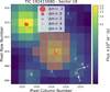 |
Fig. B.1 TESS Sector 18 target pixel file image, produced with <mono>tpfplotter</mono> (Aller et al. 2020). The image displays electron counts, with red-contoured pixels indicating the SPOC aperture mask. Red circles mark the primary target (labeled as 1) and nearby sources (labeled with other numbers) at their Gaia DR3 positions. The size of each circle represents the relative brightness of the corresponding source compared to the target star. Arrows illustrate the proper motion of each star. |
Appendix C Period alias analysis
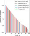 |
Fig. C.1 Log probabilities for individual aliases below 100 d from MonoTools analysis. Dark red bars show aliases ruled out by CHEOPS non-detections. Light red bars show aliases ruled out by the initial CHEOPS transit (at t3 = 2460254.82; also identical to the alias constraints from the additional TESS transit at t5 = 2460619.47). Light blue bars show potential aliases after the third transit. The dark blue bar (Pb ∼ 52 d) shows the only other remaining alias after the second CHEOPS transit detection (at t4 = 2460306.92), and the green bar shows the true period confirmed by the third CHEOPS transit observation (at t6 = 2460645.53). Only solutions with P < 100 d are shown. |
Appendix D High-resolution image
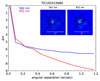 |
Fig. D.1 Contrast curves for speckle interferometry observations of TOI-6041 are represented by blue and red solid lines, corresponding to the 562 nm and 832 nm bands, respectively. The plot also features the final reconstructed images, which are exhibited in the upper right corner. |
Appendix E RV time series
APF RVs for TOI-6041
SOPHIE RVs for TOI-6041
Appendix F Periodogram on SAP TESS data
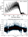 |
Fig. F.1 Rotation period analysis from the SAP TESS light curve, after masking transits of TOI-6041 b. Top: Lomb-Scargle periodogram showing a broad, significant peak between 20–30 d, under the 0.001% FAP. Bottom: Light curve phase-folded on the best-fit period (∼23 d), with the model overplotted in red. This analysis was performed using the <mono>Astropy</mono> library. |
Appendix G Age probability distribution function
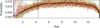 |
Fig. G.1 Posterior probability distribution for stellar age from the EXO-FASTv2 fit (see Sect. 4.2). Each color represents an individual MCMC chain, with the thick black curve showing the average across all chains. The thin black vertical line marks the best value. |
Appendix H TTVs of TOI-6041 b
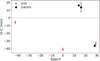 |
Fig. H.1 TTV observed–calculated (O–C) diagram for TOI-6041b. The transit times are calculated using a linear ephemeris model, Tc = T0 + E · P, with T0 = 2459890.114417 ± 0.000467 BJD and P = 26.049584 ± 2.37 × 10⁻⁵ d, where E represents the transit epoch. These values are derived by minimizing the covariance between T0 and P, following the approach described in Eastman et al. (2019). |
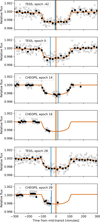 |
Fig. H.2 TOI-6041 TESS and CHEOPS photometric data, overplotted by the joint modeling including the TTV fit using the <mono>EXOFASTv2</mono>. The data points are plotted in gray, with the black points representing the binned data: 20-minute bins for the TESS data and 9-minute bins for the CHEOPS data. The best-fit transit models are displayed in orange. Vertical blue lines show the expected linear mid-transit times, and vertical orange lines mark the measured mid-transit times; both include their respective 1σ error bars. The transit epoch is labeled in the top-left corner of each plot. |
Appendix I Wavelength, telescope, and transit parameters derived from <mono>EXOFASTv2</mono> fit
Wavelength, telescope, and transit parameters derived from <mono>EXOFASTv2</mono> fit.
Appendix J Different tests on the effect of a potential third planet
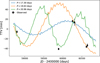 |
Fig. J.1 Transit-timing variations of TOI-6041b with a hypothetical planet placed interior to planet b. We adopt circular and coplanar orbits for all three planets and consider three orbital periods for the additional planet: 17.3 d (blue), 19.63 d (orange) and 20.96 d (green), corresponding to potential 3:2, 4:3 and 5:4 MMRs with planet b. |
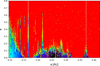 |
Fig. J.2 Possible location of an additional planet in the TOI-6041 system. The stability of a low-mass planet (K = 0.5 m/s) is analyzed as a function of semi-major axis and eccentricity. All angles are set to 0◦, except for the inclination (90◦). As in Figures 4 and 6, red regions indicate strongly chaotic orbits, while dark blue regions correspond to long-term stability. White dashed lines indicate the nominal orbital periods of planets b and c. |
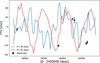 |
Fig. J.3 Transit-timing variations of TOI-6041b with a hypothetical planet placed between planets b and c. We adopt circular and coplanar orbits for all three planets and consider two orbital periods for the additional planet: 36 d (blue) and 41 d (red), corresponding to potential 4:3 and 3:2 MMRs with planet b. In both cases, the resulting TTV amplitudes are consistent with the observed variations. |
All Tables
Comparison of different models tested using RV-only data analyzed with <mono>juliet</mono>.
Wavelength, telescope, and transit parameters derived from <mono>EXOFASTv2</mono> fit.
All Figures
|
Fig. 1 Spectral energy distribution of TOI-6041. Red symbols represent the observed photometric measurements, where the horizontal bars represent the effective width of the pass band. Blue symbols show the model fluxes from the best-fit PHOENIX atmosphere model (black). The absolute flux-calibrated Gaia spectrum is shown as a gray swathe in the inset figure. |
| In the text | |
|
Fig. 2 Periodograms of RV and S-index derived from APF data for TOI-6041. From top to bottom: APF RVs, residuals of the RVs after a Keplerian fit to the 88 d signal, and the S-index activity indicator. The vertical pink line marks the planet candidate with a period of 88 d, which shows no corresponding signal in the S-index periodogram. The horizontal lines indicate false alarm probability (FAP; Baluev 2008) thresholds of 0.1%, 1%, and 10%, respectively, from top to bottom. |
| In the text | |
|
Fig. 3 APF RV measurements of TOI-6041 (top panel); phase-folded RVs for TOI-6041c (second panel) and TOI-6041b (third panel); and the phase-folded CHEOPS and TESS light curves for TOI-6041b (fourth and fifth panels). The red lines show the best-fit models derived using EXOFASTv2. Residuals are displayed at the bottom of each panel. |
| In the text | |
|
Fig. 4 Stability analysis of TOI-6041 system. The phase space of the system is explored by varying the orbital period, Pi, and eccentricity, ei, of each planet independently. For each initial condition (Table 4), the system is integrated over 10 kyr, and a stability criterion is derived with the frequency analysis of the mean longitude. The chaotic diffusion is measured by the variation in the frequencies. The color-scale corresponds to the logarithmic variation in the stability index used in Correia et al. (2010). The red zone corresponds to highly unstable orbits, while the dark blue region can be assumed to be stable on a billion-year timescale. Dashed white lines indicate the nominal orbital periods reported in Table 4. |
| In the text | |
|
Fig. 5 Transit-timing variations of TOI-6041b planet. We adopted ec = 0.3 and two values of the argument of pericenter: ωc = 0◦ (blue) and ωc = 50◦ (red). All other parameters are fixed at their nominal values from Table 4. The dots correspond to the observed TTVs. While the amplitudes are consistent with observations, the signal shape depends strongly on the orbital phase angles. |
| In the text | |
|
Fig. 6 Stability analysis of TOI-6041 system in the (Ωc, ic) plane. The phase space is explored by varying these two parameters, while all other orbital elements are fixed to the nominal values in Table 4. As in Fig. 4, red regions indicate strongly chaotic orbits, while dark blue regions correspond to long-term stability. White curves denote levels of constant mutual inclination between planets b and c. |
| In the text | |
|
Fig. 7 Transit-timing variations of TOI-6041b in a three-planet model including the hypothetical 11 d planet. We adopted the same favorable configuration as in Fig. 5, with ec = 0.3 and ωc = 50◦, and varied the eccentricity of the additional planet, e, from 0 to 0.4. The resulting curves show negligible differences, confirming that planet c likely is the dominant source of the observed TTVs in this configuration. |
| In the text | |
|
Fig. 8 Location of TOI-6041 b within radius–period diagram, along with other known exoplanets whose radius precision is better than 30%, taken from the NASA Exoplanet Archive (https://exoplanetarchive.ipac.caltech.edu/) as of June 5, 2025. The background-density map illustrates the distribution of confirmed exo-planets, with regions labeled as the desert, ridge, and savanna to reflect differing planet-occurrence rates (Castro-González et al. 2024). TOI-6041 b (green marker) lies in the savanna region. This plot was generated using the <mono>nep-des</mono> Python code (https://github.com/castro-gzlz/nep-des). |
| In the text | |
|
Fig. B.1 TESS Sector 18 target pixel file image, produced with <mono>tpfplotter</mono> (Aller et al. 2020). The image displays electron counts, with red-contoured pixels indicating the SPOC aperture mask. Red circles mark the primary target (labeled as 1) and nearby sources (labeled with other numbers) at their Gaia DR3 positions. The size of each circle represents the relative brightness of the corresponding source compared to the target star. Arrows illustrate the proper motion of each star. |
| In the text | |
|
Fig. C.1 Log probabilities for individual aliases below 100 d from MonoTools analysis. Dark red bars show aliases ruled out by CHEOPS non-detections. Light red bars show aliases ruled out by the initial CHEOPS transit (at t3 = 2460254.82; also identical to the alias constraints from the additional TESS transit at t5 = 2460619.47). Light blue bars show potential aliases after the third transit. The dark blue bar (Pb ∼ 52 d) shows the only other remaining alias after the second CHEOPS transit detection (at t4 = 2460306.92), and the green bar shows the true period confirmed by the third CHEOPS transit observation (at t6 = 2460645.53). Only solutions with P < 100 d are shown. |
| In the text | |
|
Fig. D.1 Contrast curves for speckle interferometry observations of TOI-6041 are represented by blue and red solid lines, corresponding to the 562 nm and 832 nm bands, respectively. The plot also features the final reconstructed images, which are exhibited in the upper right corner. |
| In the text | |
|
Fig. F.1 Rotation period analysis from the SAP TESS light curve, after masking transits of TOI-6041 b. Top: Lomb-Scargle periodogram showing a broad, significant peak between 20–30 d, under the 0.001% FAP. Bottom: Light curve phase-folded on the best-fit period (∼23 d), with the model overplotted in red. This analysis was performed using the <mono>Astropy</mono> library. |
| In the text | |
|
Fig. G.1 Posterior probability distribution for stellar age from the EXO-FASTv2 fit (see Sect. 4.2). Each color represents an individual MCMC chain, with the thick black curve showing the average across all chains. The thin black vertical line marks the best value. |
| In the text | |
|
Fig. H.1 TTV observed–calculated (O–C) diagram for TOI-6041b. The transit times are calculated using a linear ephemeris model, Tc = T0 + E · P, with T0 = 2459890.114417 ± 0.000467 BJD and P = 26.049584 ± 2.37 × 10⁻⁵ d, where E represents the transit epoch. These values are derived by minimizing the covariance between T0 and P, following the approach described in Eastman et al. (2019). |
| In the text | |
|
Fig. H.2 TOI-6041 TESS and CHEOPS photometric data, overplotted by the joint modeling including the TTV fit using the <mono>EXOFASTv2</mono>. The data points are plotted in gray, with the black points representing the binned data: 20-minute bins for the TESS data and 9-minute bins for the CHEOPS data. The best-fit transit models are displayed in orange. Vertical blue lines show the expected linear mid-transit times, and vertical orange lines mark the measured mid-transit times; both include their respective 1σ error bars. The transit epoch is labeled in the top-left corner of each plot. |
| In the text | |
|
Fig. J.1 Transit-timing variations of TOI-6041b with a hypothetical planet placed interior to planet b. We adopt circular and coplanar orbits for all three planets and consider three orbital periods for the additional planet: 17.3 d (blue), 19.63 d (orange) and 20.96 d (green), corresponding to potential 3:2, 4:3 and 5:4 MMRs with planet b. |
| In the text | |
|
Fig. J.2 Possible location of an additional planet in the TOI-6041 system. The stability of a low-mass planet (K = 0.5 m/s) is analyzed as a function of semi-major axis and eccentricity. All angles are set to 0◦, except for the inclination (90◦). As in Figures 4 and 6, red regions indicate strongly chaotic orbits, while dark blue regions correspond to long-term stability. White dashed lines indicate the nominal orbital periods of planets b and c. |
| In the text | |
|
Fig. J.3 Transit-timing variations of TOI-6041b with a hypothetical planet placed between planets b and c. We adopt circular and coplanar orbits for all three planets and consider two orbital periods for the additional planet: 36 d (blue) and 41 d (red), corresponding to potential 4:3 and 3:2 MMRs with planet b. In both cases, the resulting TTV amplitudes are consistent with the observed variations. |
| In the text | |
Current usage metrics show cumulative count of Article Views (full-text article views including HTML views, PDF and ePub downloads, according to the available data) and Abstracts Views on Vision4Press platform.
Data correspond to usage on the plateform after 2015. The current usage metrics is available 48-96 hours after online publication and is updated daily on week days.
Initial download of the metrics may take a while.