| Issue |
A&A
Volume 707, March 2026
|
|
|---|---|---|
| Article Number | A141 | |
| Number of page(s) | 11 | |
| Section | Atomic, molecular, and nuclear data | |
| DOI | https://doi.org/10.1051/0004-6361/202557067 | |
| Published online | 11 March 2026 | |
Theoretical investigation of transition data of astrophysical importance in neutral sulphur
1
State Key Laboratory of Solar Activity and Space Weather, National Astronomical Observatories, Chinese Academy of Sciences,
PR China
2
Theoretical Astrophysics, Department of Physics and Astronomy, Uppsala University,
Box 516,
751 20
Uppsala,
Sweden
3
Department of Materials Science and Applied Mathematics, Malmö University,
205 06
Malmö,
Sweden
★ Corresponding author: This email address is being protected from spambots. You need JavaScript enabled to view it.
Received:
2
September
2025
Accepted:
26
January
2026
Abstract
Accurate and comprehensive atomic data are essential for the modelling of stellar spectra. Uncertainties in the oscillator strengths of specific lines used for abundance analyses directly translate into uncertainties in the derived elemental abundances; incomplete or biased atomic data sets can impart significant errors in non-local thermodynamic equilibrium (non-LTE) modelling. Theoretical calculations of atomic data are therefore crucial to supplement the limited experimental results. In this work, we present extensive atomic data, including oscillator strengths, transition rates, and lifetimes for 1730 electric-dipole (E1) transitions among 107 levels in neutral sulphur (S I) using the multi-configuration Dirac–Hartree–Fock (MCDHF) and relativistic-configuration-interaction (RCI) methods. These levels belong to the configurations 3p3np (n = 3 − 7), 3p3nf (n = 4, 5), 3s3p5, 3p3ns (n = 4 − 7), and 3p3nd (n = 3 − 6). The accuracy of the computed transition rates is assessed by combining the comparison of the differences in transition rates between the Babushkin and Coulomb gauges with a cancellation-factor (CF) analysis. Approximately 16% of the ab initio results achieved an accuracy classification of A–B, corresponding to uncertainties within 10%, as defined by the Atomic Spectra Database of the National Institute of Standards and Technology (NIST ASD). Applying a fine-tuning technique was found to significantly improve the accuracy of the results in the Coulomb gauge, thereby improving the consistency between the Babushkin and Coulomb gauges; about 24% of the fine-tuned transition data are assigned to the accuracy classes A–B.
Key words: atomic data / atomic processes
© The Authors 2026
 Open Access article, published by EDP Sciences, under the terms of the Creative Commons Attribution License (https://creativecommons.org/licenses/by/4.0), which permits unrestricted use, distribution, and reproduction in any medium, provided the original work is properly cited.
This article is published in open access under the Subscribe to Open model. This email address is being protected from spambots. You need JavaScript enabled to view it. to support open access publication.
1 Introduction
Spectroscopy is a powerful tool in astrophysics, providing critical insights into the physical conditions and chemical abundances of stars (Tennyson 2019). Sulphur, as one of the most abundant elements in the Universe, exhibits a wealth of spectral features across multiple wavelength bands that have been observed with both space- and ground-based facilities (e.g. Durrance et al. 1983; Skillman & Kennicutt 1993; Carpenter et al. 1994). These lines serve as powerful diagnostics for probing stellar atmospheres, the interstellar medium, and galaxies (e.g. Judge 1988; Feaga et al. 2002; Anderson et al. 2013). In particular, as an α element, sulphur is routinely employed in the study of Galactic chemical evolution (e.g. Nissen et al. 2007; Skúladóttir et al. 2015; Duffau et al. 2017; Costa Silva et al. 2020; da Silva et al. 2023).
Given this importance, it is of interest to reliably infer sulphur abundances in stars and in other astronomical objects. However, accurate analyses of observed sulphur spectra require accurate and complete atomic data sets. Errors in transition data of small sets of diagnostic lines directly impact inferred sulphur abundances; while incomplete or systematically biased atomic data sets could impact the statistical equilibrium in non-local thermodynamic equilibrium (non-LTE) models (e.g. Kamp et al. 2001; Daflon et al. 2003; Takeda et al. 2005; Korotin & Kiselev 2024). Considerable effort has therefore been devoted to both theoretical calculations and laboratory measurements of transition data for neutral sulphur.
On the experimental side, earlier measurements of oscillator strength and transition probabilities between multiplet transitions were reported by Savage & Lawrence (1966), Bridges & Wiese (1967), and Müller (1968). Doering (1990) measured relative oscillator strengths for the 3p4 3P − 3p3(4S)4s 3So (1814 Å), 3p4 3P − 3p3(2D)4s 3Do (1479 Å), and 3p4 3P − 3p3(4S)3d 3Do (1429 Å) multiplets using the method of electron energy-loss spectroscopy. Delalic et al. (1990) determined the radiative lifetimes of eight different multiplets in the visible range using the high-frequency deflection technique. Beideck et al. (1994) derived oscillator strengths for eight transitions of the multiplets between ![Mathematical equation: $\[3 \mathrm{p}^{3}({ }^{4} \mathrm{S}) 4 \mathrm{s}~^{3} \mathrm{S}^\mathrm{o}, 3 \mathrm{p}^{3}({ }^{2} \mathrm{P}) 4 \mathrm{s}~^{3} \mathrm{P}^\mathrm{o}\]$](/articles/aa/full_html/2026/03/aa57067-25/aa57067-25-eq1.png) , and 3p4 3P based on measured mean lifetimes and branching ratios using beam-foil spectroscopic techniques at the Toledo Heavy Ion Accelerator. Based on the oscillator strength reported by Doering (1990) and Beideck et al. (1994), Federman & Cardelli (1995) analysed interstellar spectra towards ζ-Oph acquired with the Goddard High-Resolution Spectrograph and obtained a self-consistent set of oscillator strengths for approximately a dozen S I lines from a curve of growth. More recently, using time-resolved vacuum-ultraviolet laser spectroscopy, Zerne et al. (1997) determined oscillator strengths for the
, and 3p4 3P based on measured mean lifetimes and branching ratios using beam-foil spectroscopic techniques at the Toledo Heavy Ion Accelerator. Based on the oscillator strength reported by Doering (1990) and Beideck et al. (1994), Federman & Cardelli (1995) analysed interstellar spectra towards ζ-Oph acquired with the Goddard High-Resolution Spectrograph and obtained a self-consistent set of oscillator strengths for approximately a dozen S I lines from a curve of growth. More recently, using time-resolved vacuum-ultraviolet laser spectroscopy, Zerne et al. (1997) determined oscillator strengths for the ![Mathematical equation: $\[3 \mathrm{p}^{3}({ }^{4} \mathrm{S}) 4 \mathrm{s}~^{3} \mathrm{S}_{1}^\mathrm{o}{-}3 \mathrm{p}^{3}({ }^{4} \mathrm{S}) 4 \mathrm{p}~^{3} \mathrm{P}_{0,1,2}\]$](/articles/aa/full_html/2026/03/aa57067-25/aa57067-25-eq2.png) triplet at 10 450 Å and Berzinsh et al. (1997) reported lifetimes for twelve states. These lifetime data were combined by Biémont et al. (1998) with their theoretical branching ratios from relativistic Hartree–Fock (HFR) calculations to deduce a consistent set of oscillator strengths for vacuum ultraviolet lines.
triplet at 10 450 Å and Berzinsh et al. (1997) reported lifetimes for twelve states. These lifetime data were combined by Biémont et al. (1998) with their theoretical branching ratios from relativistic Hartree–Fock (HFR) calculations to deduce a consistent set of oscillator strengths for vacuum ultraviolet lines.
Besides experimental measurements, there are also a number of theoretical calculations of the transition data for S I. Ganas (1982) calculated the optical oscillator strengths for the sulphur isoelectric sequence using an analytic atomic independent-particle-model potential. Kurucz & Peytremann (1975) calculated the oscillator strength semi-empirically using scaled Thomas-Fermi-Dirac radial wave functions and eigenvectors found through least-squares fits to observed energy levels. Ho & Henry (1985), Fleming & Hibbert (1999), Tayal (1998), and Chen & Msezane (1997) did the calculations using the CIV3 code based on configuration-interaction (CI) method (Hibbert 1975). Fawcett (1986) calculated the oscillator strengths for allowed n=3–3 and 3–4 transitions of S I with the HFR program package. Fischer (1987) carried out multi-configuration Hartree–Fock (MCHF) calculations for a number of 3p3(2D)nd 3Po terms in S I. More recently, Froese Fischer et al. (2006) reported both allowed electricdipole (E1) and some forbidden transitions among levels up to ![Mathematical equation: $\[3 \mathrm{p}^{3}({ }^{4} \mathrm{S}) 3 \mathrm{d}~^{3} \mathrm{D}^\mathrm{o}\]$](/articles/aa/full_html/2026/03/aa57067-25/aa57067-25-eq3.png) by including relativistic effects through the Breit–Pauli Hamiltonian. Zatsarinny & Bartschat (2006), hereafter ZB2006 reported fine structure energies for configurations 3p3nl of certain levels up to n=12 and the associated E1 oscillator strengths among them using a B-spline box-based multi-channel method. In this calculation, they included CI effects by using a fairly large B-spline basis set and relativistic effects through the Breit–Pauli Hamiltonian. Deb & Hibbert (2006) and Deb & Hibbert (2008), hereafter DH2008 presented oscillator strengths and radiative rates for 2173 E1 transitions among 120 levels using the CIV3 program with a fine-tuning technique. However, as reported by ZB2006, comparisons of oscillator strengths and transition probabilities among various calculations sometimes show large disagreement. The large disagreement between different calculations indicates large uncertainties in the theoretical atomic data, which may have a significant impact on astrophysical spectroscopic analyses. This may be due to the insufficient configuration interactions included in many of the calculations. The most recent work by DH2008 included 300 000 configuration state functions (CSFs) in their CI calculation, which, to our knowledge, is the largest scale calculation for S I to date. However, larger scale calculations, such as those with millions of CSFs, had not been performed until now.
by including relativistic effects through the Breit–Pauli Hamiltonian. Zatsarinny & Bartschat (2006), hereafter ZB2006 reported fine structure energies for configurations 3p3nl of certain levels up to n=12 and the associated E1 oscillator strengths among them using a B-spline box-based multi-channel method. In this calculation, they included CI effects by using a fairly large B-spline basis set and relativistic effects through the Breit–Pauli Hamiltonian. Deb & Hibbert (2006) and Deb & Hibbert (2008), hereafter DH2008 presented oscillator strengths and radiative rates for 2173 E1 transitions among 120 levels using the CIV3 program with a fine-tuning technique. However, as reported by ZB2006, comparisons of oscillator strengths and transition probabilities among various calculations sometimes show large disagreement. The large disagreement between different calculations indicates large uncertainties in the theoretical atomic data, which may have a significant impact on astrophysical spectroscopic analyses. This may be due to the insufficient configuration interactions included in many of the calculations. The most recent work by DH2008 included 300 000 configuration state functions (CSFs) in their CI calculation, which, to our knowledge, is the largest scale calculation for S I to date. However, larger scale calculations, such as those with millions of CSFs, had not been performed until now.
The purpose of this study is to present the results of our extensive calculations using the fully relativistic multi-configuration Dirac–Hartree–Fock (MCDHF) and relativistic configuration interaction (RCI) methods. Here we provide two sets of calculation results. One set was obtained directly from the MCDHF and RCI calculations, which we refer to as the ab initio results. The other set involves fine-tuning of eigenvalues in the RCI calculations, which we refer to as the fine-tuned results. We compare the fine-tuned data with the ab initio results to investigate the effects of fine-tuning on radiative data and lifetimes. The new atomic data set may help with assessing the accuracy of various atomic data via comparisons with other data sets.
This paper is structured into four sections, including the Introduction. Section 2 introduces the theoretical methods and computational schemes. Section 3 presents the results and discussions on energy levels, transition data, and lifetimes. Section 4 includes our conclusion.
2 Method
2.1 Multi-configuration Dirac–Hartree–Fock approach
The calculations were performed using the MCDHF and RCI methods, based on a Dirac–Coulomb Hamiltonian, which are implemented in the general-purpose relativistic atomic-structure package GRASP20181. We briefly outline the methods in this section and refer the reader to Grant (2007), Froese Fischer et al. (2016), Froese Fischer et al. (2019), and Jönsson et al. (2023b) for details of the MCDHF method and Jönsson et al. (2023a) for a step-by-step instruction manual of the package.
In the MCDHF method, the atomic state wave functions (ASFs, Ψ(γ(j) PJM)) are expanded over a linear combination of configuration state functions (CSFs, Φ(γi PJM)):
![Mathematical equation: $\[\Psi(\gamma^{(j)} P J M)=\sum_i^{N_{\text {CSFs }}} c_i^{(j)} ~\Phi(\gamma_i P J M).\]$](/articles/aa/full_html/2026/03/aa57067-25/aa57067-25-eq4.png) (1)
(1)
The CSFs are jj-coupled multi-electron functions built from products of one-electron Dirac orbitals. The radial parts of the one-electron orbitals and the expansion coefficients of the CSFs are obtained in a relativistic self-consistent field procedure by solving the Dirac–Hartree–Fock radial equations and the configuration interaction eigenvalue problem. The angular integrations needed for the construction of the energy functional are based on the second quantisation method in the coupled tensorial form (Gaigalas et al. 1997, 2001). Once the radial components of the one-electron orbitals are determined, in the following RCI calculations, higher order interactions, such as the Breit interaction and quantum electrodynamic effects (self-energy and vacuum polarization), are added to the Dirac–Coulomb Hamiltonian. Keeping the radial components fixed, the expansion coefficients of the CSFs for the target states are obtained by solving the configuration interaction eigenvalue problem.
Once the ASFs have been determined from RCI calculations, the radiative E1 transition data (e.g. transition rates A and weighted oscillator strengths log(gf)) between two states, γ′P′J′ and γPJ, can be computed in terms of reduced matrix elements of the transition operator by summing up reduced matrix elements between all the CSFs for the lower and upper states:
![Mathematical equation: $\[\langle\Psi(\gamma P J)\|\mathbf{T}^{(1)}\| \Psi(\gamma^{\prime} P^{\prime} J^{\prime})\rangle=\sum_{j, k} c_j c_k^{\prime}~\langle\Phi(\gamma_j P J)\|\mathbf{T}^{(1)}\| \Phi(\gamma_k^{\prime} P^{\prime} J^{\prime})\rangle.\]$](/articles/aa/full_html/2026/03/aa57067-25/aa57067-25-eq5.png) (2)
(2)
The transition operator can be expressed in the Babushkin and Coulomb gauges, which in the non-relativistic limit, respectively, correspond to the length and velocity forms. In the limit of including CSFs obtained by all possible excitations to a complete set of orbitals, we may arrive at the exact wave functions to the Dirac equation; this leads to identical values for the Babushkin and Coulomb transition moments (Grant 1974). However, when approximate multi-electron wave functions are used in practice, the transition data in the two gauges are often different. The relative difference between the values of these two gauges, dT = |AB − AC|/max(AB, AC), can be used as one indicator of the accuracy of the wave functions (Froese Fischer 2009; Ekman et al. 2014). It should be noted that dT should be used in a statistical manner as done in Papoulia et al. (2019) and Li et al. (2023a,b). We discuss this further in Section 3.2.1.
In the MCDHF relativistic calculations, the ASFs are given in terms of jj-coupled CSFs. In order to identify the computed states and adapt the labelling conventions followed by the astronomers and experimentalists, the ASFs are transformed from jj-coupling to a basis of LSJ-coupled CSFs. In the GRASP2018 package, the transformation from jj- to LSJ-coupling is done by the jj21sj program developed by Gaigalas et al. (2003, 2004, 2017).
Summary of the computational schemes for S I.
2.2 Computational schemes
We targeted the states belonging to the {3p3np (n = 3 − 7), 3p3nf (n = 4, 5)} even configurations and the {3s3p5, 3p3ns (n = 4 − 7), 3p3nd (n = 3 − 6)} odd configurations. To account for higher order configuration–interaction contributions in the wave functions relative to the target configurations, we employed extended multi-reference (MR) configurations in both MCDHF (MR-MCDHF) and RCI (MR-RCI) calculations. These extended MR sets were determined through the rcsfmr program in GRASP2018 based on the results of a preliminary calculation. The final MR sets adopted in the MCDHF and RCI calculations, the orbital sets, and the total number of CSFs (NCSFs) for even and odd parities are presented in Table 1.
Our calculations were performed in the extended optimal level scheme (Dyall et al. 1989) for the weighted average of the even and odd parity states. The multi-reference single-double (MR-SD) method was employed to obtain CSF expansions, which allows for single and double (SD) substitutions from MR configurations to orbitals within an active set (AS; Olsen et al. 1988; Sturesson et al. 2007; Froese Fischer et al. 2016). The orbitals in the AS are divided into spectroscopic orbitals, which build the configurations in the MR, and correlation orbitals, which are introduced to correct the initially obtained wave functions. 1s22s22p6 was always kept as an inactive closed core. In the MCDHF calculations, the 3s orbitals were kept inactive and the CSF expansions were produced by SD substitutions from all the other valence orbitals of the configurations in the MR-MCDHF. The final wave functions of the target states were determined in a subsequent RCI calculation, which included CSF expansions that were formed by allowing SD substitution from the n ≥ 3 sub-shells of the MR-MCDHF configurations and single substitution from the n ≥ 3 sub-shells of the additional configurations in the MR-RCI to the active sets of orbitals presented in Table 1. Breit interactions were also taken into account in the RCI calculation. The final even and odd state expansions, respectively, contained 11 049 420 and 8 146 099 CSFs, distributed over different J symmetries (0–5 for even parity and 0–4 for odd parity).
2.3 Fine-tuning
In atomic-structure calculations, fine-tuning or adjustment of the diagonal elements of the Hamiltonian matrix based on experimental energies is a powerful semi-empirical technique that can substantially reduce the deviations between theoretical and experimentally observed energy levels. This technique has been implemented in the CIV3 (Hibbert 1975) program based on the CI method and in the ATSP2K (Froese Fischer et al. 2007) program based on the MCHF method. It has been successfully applied to the calculations of several atomic systems to obtain accurate energy levels and transition parameters (e.g. Lundberg et al. 2001; Corrégé & Hibbert 2004; Froese Fischer & Tachiev 2004). Both of the above methods are based on LSJ-coupled configuration state functions, where the off-diagonal matrix elements between different LS-terms are small. However, applying fine-tuning directly to jj-coupled calculations is challenging due to the large off-diagonal matrix elements. To address this issue, Li et al. (2023) proposed a method to convert the Hamiltonian from jj-coupling to one in LSJ-coupling, where fine-tuning can be applied, and return to the jj-coupling form. The procedure was successfully implemented in GRASP2018 through two new programs jj2lsj_2022 and rfinetune. They also demonstrated that fine-tuning, using C III and B I as examples, significantly improved the accuracy of transition rates and lifetimes, showing clear improvements compared to ab initio calculations. The LS-composition analysis of the ab initio results reveals that, with a few exceptions in 3p3(4S)7p 3P and 3s3p5 3P states, most states in S I can be well described with relatively pure LSJ-coupling. Therefore, we adopted the same approach as that employed in Li et al. (2023).
In this work, we applied our fine-tuning procedure for the even and odd states using the MR-RCI set, based on experimental energies from the Atomic Spectra Database of the National Institute of Standards and Technology (NIST ASD) (Kramida et al. 2024). It should be noted that while we were preparing the paper, NIST ASD updated the energy levels based on the results from Civiš et al. (2024). Upon careful comparison, we found that the corrections on the energy levels were negligible, with most relative differences being of the order of 10−7. The largest correction occurred in the 3p3(4S)7p 5P3, with a relative difference of 10−4. Such small differences will not have significant impacts on our fine-tuning results. Therefore, we retained the fine-tuning results in this work.
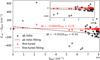 |
Fig. 1 Energy differences as a function of excitation energies provided by NIST ASD. The dashed black and red lines are the linear fit to the data from ab initio (black plus) and fine-tuning (red plus) calculations, respectively. The inset in the upper right shows an enlarged view for ENIST > 5 × 104 cm−1. |
3 Results and discussions
3.1 Energy levels
The energy levels for the 107 lowest states of S I (56 even states and 51 odd states) from both ab initio and fine-tuning calculations are presented in Table A.1, together with the experimental energies from the recent update of the NIST ASD by Civiš et al. (2024). The numbers in the first column of the table, labelled as ‘No.’ are in the order of the energy levels given in the NIST ASD. Figure 1 shows the energy differences between calculated data and NIST ASD values plotted against the excitation energies, ENIST. The agreement between the computational and experimental energies is systematically improved after fine-tuning; the systematic error of computational excitation energies decreases from 0.22% to 0.03%, and the root-mean-square deviation decreases from 188.5 cm−1 to 20.3 cm−1. Especially for the energy levels of ![Mathematical equation: $\[3 \mathrm{p}^{4}~{ }^{1} \mathrm{S}_{0}, 3 \mathrm{p}^{3}({ }^{4} \mathrm{S}) 4 \mathrm{s}~^{5} \mathrm{S}_{2}^\mathrm{o},{ }^{3} \mathrm{S}_{1}^\mathrm{o}\]$](/articles/aa/full_html/2026/03/aa57067-25/aa57067-25-eq6.png) , and 3p3(4S)4p 5P1,2,3,3 P0,1,2, the ab initio energies are rather far away (more than 300 cm−1) from the experimental energies; in contrast, the fine-tuned energies are all within 50 cm−1 of the experimental values, except for 3p4 1S0, which differs by 96 cm−1. In addition, fine-tuning can help correct the energy positions of the levels, where the positions refer to the level locations arranged in terms of the excitation energies. For example, in the ab initio calculation, the
, and 3p3(4S)4p 5P1,2,3,3 P0,1,2, the ab initio energies are rather far away (more than 300 cm−1) from the experimental energies; in contrast, the fine-tuned energies are all within 50 cm−1 of the experimental values, except for 3p4 1S0, which differs by 96 cm−1. In addition, fine-tuning can help correct the energy positions of the levels, where the positions refer to the level locations arranged in terms of the excitation energies. For example, in the ab initio calculation, the ![Mathematical equation: $\[3 \mathrm{p}^{3}({ }^{2} \mathrm{P}) 4 \mathrm{s}~^{1} \mathrm{P}_{1}^{\mathrm{o}}\]$](/articles/aa/full_html/2026/03/aa57067-25/aa57067-25-eq7.png) state is higher than the 3p3(2D)4p 3F states and in the wrong position compared to experimental data. Fine-tuning brings the energy into the correct position with a corresponding slightly decreased mixing with the
state is higher than the 3p3(2D)4p 3F states and in the wrong position compared to experimental data. Fine-tuning brings the energy into the correct position with a corresponding slightly decreased mixing with the ![Mathematical equation: $\[3 \mathrm{p}^{3}({ }^{2} \mathrm{D}) 3 \mathrm{d}~^{1} \mathrm{P}_{1}^\mathrm{o}\]$](/articles/aa/full_html/2026/03/aa57067-25/aa57067-25-eq8.png) perturber into the
perturber into the ![Mathematical equation: $\[3 \mathrm{p}^{3}({ }^{2} \mathrm{P}) 4 \mathrm{s}~^{1} \mathrm{P}_{1}^\mathrm{o}\]$](/articles/aa/full_html/2026/03/aa57067-25/aa57067-25-eq9.png) state.
state.
Further iterations of fine-tuning could potentially yield results even closer to the experimental energies. Considering the total time cost involved in the fine-tuning process and the recalculation of the wave functions and transition properties, as well as the fact that currently available results have already reached a level of accuracy that is challenging to attain simply by increasing the size of the CSF basis, especially given that the present work involved over ten million CSFs in the calculations, we believe that the current results are sufficient to study the impact of fine-tuning on transition data.
3.2 Transition data
The transition parameters computed from both ab initio and fine-tuning calculations for 1730 E1 transitions among the 107 energy levels given in Table A.1 are presented in Table A.2; the full table is available at the CDS. Note that the wavelengths listed in all tables of the paper are derived from the experimental energy levels in the NIST ASD, which are originally from Civiš et al. (2024); the transition data, including weighted oscillator strengths, log(gf) and transition rates, A, for both ab initio and fine-tuned results are all adjusted using experimental wavelengths.
3.2.1 Accuracy assessment
We evaluated the accuracy of our computed transition data following the method used in Li et al. (2023b). This approach is based on grouping transitions based on the magnitude of A values. For S I, we chose six groups such that A < 10−2 s−1, 10−2 ≤ A < 100 s−1, 100 ≤ A < 103 s−1, 103 ≤ A < 3.5 × 10⁵ s−1, 3.5 × 10⁵ ≤ A < 107 s−1, and A ≥ 107. Next, we calculated the averaged dTav for each group. As we mentioned in Section 2.1, the gauge difference parameter should only be used as an uncertainty estimate in a statistical manner for a group of transitions with similar properties. As such, we define ![Mathematical equation: $\[\mathrm{d} \tilde{T}\]$](/articles/aa/full_html/2026/03/aa57067-25/aa57067-25-eq10.png) as max(dT, dTav) to replace dT as the gauge difference indicator for individual transitions. We then folded the cancellation-factor (CF) into the analysis. This is a numerical measure of the cancellation effect in the computation of transition matrix elements (e.g. Cowan 1981; Zhang et al. 2013; Gaigalas et al. 2020). A small CF (generally under about 0.1 or 0.05 as given in Cowan 1981) indicates a strong cancellation effect, resulting in computed transition parameters with large uncertainties.
as max(dT, dTav) to replace dT as the gauge difference indicator for individual transitions. We then folded the cancellation-factor (CF) into the analysis. This is a numerical measure of the cancellation effect in the computation of transition matrix elements (e.g. Cowan 1981; Zhang et al. 2013; Gaigalas et al. 2020). A small CF (generally under about 0.1 or 0.05 as given in Cowan 1981) indicates a strong cancellation effect, resulting in computed transition parameters with large uncertainties.
The final accuracy class for each computed transition rate was estimated by a combined analysis of the ![Mathematical equation: $\[\mathrm{d} \tilde{T}\]$](/articles/aa/full_html/2026/03/aa57067-25/aa57067-25-eq11.png) and CF parameters. Based on the above procedure, we divided the accuracy into five classes, following the definition conventions of the accuracy classification in the NIST ASD. The A, B, C, D, and E classes correspond to the {A, A+, and AA}, {B+ and B}, {C+ and C}, {D+ and D}, and E classes, respectively, as defined by the NIST ASD. The definitions of
and CF parameters. Based on the above procedure, we divided the accuracy into five classes, following the definition conventions of the accuracy classification in the NIST ASD. The A, B, C, D, and E classes correspond to the {A, A+, and AA}, {B+ and B}, {C+ and C}, {D+ and D}, and E classes, respectively, as defined by the NIST ASD. The definitions of ![Mathematical equation: $\[\mathrm{d} \tilde{T}\]$](/articles/aa/full_html/2026/03/aa57067-25/aa57067-25-eq12.png) and CF for each accuracy class are as follows:
and CF for each accuracy class are as follows:
![Mathematical equation: $\[\begin{aligned}&-\mathrm{A}(\leq 3 \%): \mathrm{d} \tilde{T} \leq 3 ~\&~ \mathrm{CF} \geq 0.1 \\&-\mathrm{B}(\leq 10 \%): 3<\mathrm{d} \tilde{T} \leq 10 ~\&~ \mathrm{CF} \geq 0.1 \text { or } \\&\qquad\quad\qquad\qquad\qquad \mathrm{d} \tilde{T} \leq 3 ~\&~ \mathrm{CF}<0.1 \\&-\mathrm{C}(\leq 25 \%): 10<\mathrm{d} \tilde{T} \leq 25 ~\&~ \mathrm{CF} \geq 0.1 \text { or } \\&\qquad\qquad\qquad\quad 3<\mathrm{d} \tilde{T} \leq 10 ~\&~ \mathrm{CF}<0.1 \\&-\mathrm{D}(\leq 50 \%): 25<\mathrm{d} \tilde{T} \leq 50 ~\&~ \mathrm{CF} \geq 0.1 \text { or } \\&\qquad\quad\qquad\qquad 10<\mathrm{d} \tilde{T} \leq 25 ~\&~ \mathrm{CF}<0.1 \\&-\mathrm{E}(>50 \%): \mathrm{d} \tilde{T}>50 \text { or } \\& \qquad\quad\qquad\qquad25<\mathrm{d} \tilde{T} \leq 50 ~\&~ \mathrm{CF}<0.1\end{aligned}\]$](/articles/aa/full_html/2026/03/aa57067-25/aa57067-25-eq13.png)
We provide the estimated accuracy class for each transition in Table A.2; these were defined based on the above procedure for both ab initio and fine-tuned results. We hope that this information can provide data users with a reference for data quality. Taking the Babushkin gauge as an example, the percentage fraction of each accuracy class is as follows:
ab initio : A: 2.1%; B: 13.8%; C: 30.0%; D: 28.6%; E: 25.5%
fine-tuned : A: 9.1%; B: 15.1%; C: 26.1%; D: 26.8%; E: 22.9%
The reason for the high proportion of lower accuracy data is that among the 1730 transition data, approximately 50% are LS-forbidden inter-combination transitions (IC), including two-electron one-photon (TEOP) transitions involving the 3s3p5 energy levels. These transitions are governed by electron correlation effects, which are difficult to calculate accurately. In high-accuracy classes A and B, over 80% of the transitions are LS-allowed, whereas in the low-accuracy classes D and E, more than 70% are LS-forbidden IC transitions.
The statistical results indicate that the proportion of high-accuracy results in classes A and B obtained from the fine-tuned calculations is higher than that from the ab initio calculations. The primary reason for this difference is that fine-tuning reduces the overall differences in the transition data between the Babushkin and Coulomb gauges.
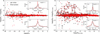 |
Fig. 2 Left: comparison of log(gf) between Babushkin and Coulomb gauges for ab initio (black plus) and fine-tuned (red plus) results, respectively. Insets (a1) and (a2) show the histograms of the log(gf) differences for transitions with log(gf) ≥ −2 and log(gf) < −2, respectively. Right: comparison of log(gf) between ab initio and fine-tuned calculations for Babushkin (black diamond) and Coulomb gauges (red hexagon), respectively. Insets (b1) and (b2) show the histograms of the log(gf) differences for transitions with log(gf) ≥ −3 and log(gf) < −3, respectively. |
3.2.2 Comparison between Babushkin and Coulomb gauges
The left panel of Figure 2 presents the differences in log(gf) values between the Babushkin and Coulomb gauges. The histograms (insets (a1) and (a2)) show the distribution of the gauge difference for transitions with log(gf) ≥ −2 and log(gf) < −2, respectively. Both the ab initio and fine-tuned data show good agreement between the two gauges, with 73% of the total of 1730 transitions differing by less than 0.1 dex. For transitions with log(gf) greater than −2.0, approximately 86% agree within 0.1 dex between the two gauges for both ab initio and fine-tuned results. In the same subset, as can be seen from the histogram (a1) in the left panel of Figure 2, the number of transitions with differences between the two gauges greater than 0.05 dex is higher for the ab initio results (33%) than for the fine-tuned results (23%). This indicates that fine-tuning can enhance the consistency between the Babushkin and Coulomb gauges to a certain degree, which accounts for the higher proportion of high-accuracy data in the fine-tuned results compared to those obtained from ab initio calculations, as demonstrated in Section 3.2.1.
Generally, stronger transitions show better agreement between the Babushkin and Coulomb gauges. However, we observed six outliers in the range of −1 to 0 of log(gf)B in Figure 2. These are transitions between high Rydberg states 3p3(4S)7p 3P0,1,2 and ![Mathematical equation: $\[3 \mathrm{p}^{3}({ }^{4} \mathrm{S}) 6 \mathrm{d}~^{3} \mathrm{D}_{1,2,3}^{\mathrm{o}}\]$](/articles/aa/full_html/2026/03/aa57067-25/aa57067-25-eq14.png) . Despite the large differences (by 1–1.5 dex) between the Babushkin and Coulomb gauges for these transitions, the ab initio and fine-tuned data in the Babushkin gauge show excellent agreement, with deviations of less than 0.01 dex, while the results in the Coulomb gauge differ by 0.2–0.5 dex. Although all six transitions are classified as E accuracy class based on the method described in Section 3.2.1, we suggest that the Babushkin gauge data may be more reliable for these transitions.
. Despite the large differences (by 1–1.5 dex) between the Babushkin and Coulomb gauges for these transitions, the ab initio and fine-tuned data in the Babushkin gauge show excellent agreement, with deviations of less than 0.01 dex, while the results in the Coulomb gauge differ by 0.2–0.5 dex. Although all six transitions are classified as E accuracy class based on the method described in Section 3.2.1, we suggest that the Babushkin gauge data may be more reliable for these transitions.
3.2.3 Comparison between ab initio and fine-tuned results
The right panel of Figure 2 presents a comparison of log(gf) values between the fine-tuned and the ab initio results. The histograms (insets (b1) and (b2)) display the distribution of the differences for transitions with log(gf) ≥ −3 and log(gf) < −3, respectively. It is important to note that all data, including wavelengths and transition data, were adjusted to match the experimental energy levels, ensuring that the differences shown in the figure are solely due to the changes in mixing coefficients caused by fine-tuning. From this comparison, we observe that fine-tuning has a significant impact on log(gf) values, with approximately 42% of the Babushkin data (and 45% of the Coulomb gauge data) showing changes greater than 0.1 dex. Second, as can be seen from the histogram (b1), the effect of fine-tuning is more pronounced on the Coulomb gauge results than on the Babushkin gauge data. For example, among transitions with log(gf) greater than −3.0, 42% of the Coulomb data show changes greater than 0.05 dex, compared to 26% of the Babushkin data. Third, fine-tuning has a more substantial effect on weak transitions than on strong transitions. The histograms show that 44% of transitions with log(gf) < −3 have a change in the Babushkin gauge greater than 0.2 dex, compared to 9% of transitions with log(gf) ≥ −3.
Despite ongoing debates concerning the choice of the appropriate gauge (e.g. Starace 1971; Hibbert 1974; Cowan 1981; Papoulia et al. 2019; Gaigalas et al. 2024), the Babushkin gauge is generally considered to yield more reliable transition results, as it better describes the outer part of the wave functions that governs the atomic transitions (Hibbert 1974). In addition, the contributions from the negative-energy states were not taken into account in the MCDHF and RCI calculations, which have negligible effects on the Babushkin gauge results but can affect the Coulomb gauge results significantly, especially for the weak IC transitions; this further suggests that the Babushkin gauge results appear to be more reliable (Chen et al. 2001). This explains the findings presented in Figure 2 and the conclusions in Sections 3.2.1 and 3.2.2, which namely show that fine-tuning can better improve the less accurate results in the Coulomb gauge, thereby enhancing the agreement between the Babushkin and Coulomb gauges and consequently improving the overall accuracy. Furthermore, the transition matrix element in Coulomb gauge contains a dependence on the transition energy, making it more sensitive to fine-tuning. For these reasons, the greater impact of fine-tuning on the Coulomb gauge than on the Babushkin gauge is expected.
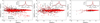 |
Fig. 3 Comparison of log(gf) from the current study with those from previous works. Left: ZB2006 (Zatsarinny & Bartschat 2006). Middle: DH2008 (Deb & Hibbert 2008). Right: NIST ASD (Kramida et al. 2024). The data in NIST ASD were compiled from various sources, including Müller (1968); Beideck et al. (1994); Biémont et al. (1996, 1998); Zerne et al. (1997); Froese Fischer et al. (2006) and Zatsarinny & Bartschat (2006). Babushkin results from present ab initio (black plus) and fine-tuned (red plus) RCI calculations are used in the comparison. The inset figures show the histograms of the distribution of the number of transitions for the differences in log(gf). Note that the y-axis range is consistent across all plots in Figures 2 and 3. |
3.2.4 Comparison with previous theoretical and experimental results
In Figure 3, our ab initio and fine-tuned log(gf) results are compared with the data from ZB2006 (1719 transitions), DH2008 (1001 transitions), and NIST ASD2 (528 transitions). ZB2006 is based on the B-spline box-based multi-channel method, while DH2008 is based on CI methods with fine-tuning. The histograms in each panel show the statistical distribution of the differences between our results and the others. Overall, our results show better agreement with ZB2006 than with DH2008. For example, among transitions with log(gf) greater than −3.0, 68.4% (66.9%) of the ab initio (fine-tuned) data agree within ±0.1 dex with ZB2006, while only 44.6% agree with DH2008.
However, some unexpected large deviations are observed in the lower right corner of the left panel in Figure 3, indicating that fine-tuning leads to large discrepancies of >1.0 dex compared with ZB2006 data for certain transitions. Most of these transitions are IC transitions between ![Mathematical equation: $\[3 \mathrm{p}^{3}({ }^{2} \mathrm{D}) 4 \mathrm{p}~^{1} \mathrm{P}, 3 \mathrm{p}^{3}({ }^{4} \mathrm{S}) \mathrm{nd}~(\mathrm{n}=3,4,5,6)~{ }^{3} \mathrm{D}^{\mathrm{o}},{ }^{5} \mathrm{D}^{\mathrm{o}}\]$](/articles/aa/full_html/2026/03/aa57067-25/aa57067-25-eq15.png) and 3p3(4S)nf (n = 3, 4, 5) 3F, 5F. IC transitions are directly caused by the mixing of states, and their theoretical transition rates are very sensitive to the quality of the wave functions; the accurate calculation of their transition data is more challenging than for LS-allowed transitions. In the upper panel of Figure 4, we compare the results of the anomalous transitions for which both ZB2006 and DH2008 data are available. As can be seen from the figure, our fine-tuned data are the largest, while our ab initio data are the smallest among all the calculated results. It is also interesting to note that, despite the considerable differences among various results, our fine-tuned data show better agreement with the fine-tuned results of DH2008, while the ab initio results are closer to ZB2006. Upon closer inspection of the energy levels associated with these ‘anomalous’ transitions, we observe no tendency for the fine-tuning process to ‘over-correct’ for inaccuracies in energy separations. In the middle and lower panels of Figure 3, we show the distribution of the dT and CF parameters. It is clear that the fine-tuned results have better consistency between the Babushkin and Coulomb gauges than the ab initio and the DH2008 results. The fine-tuned results exhibit larger CF values than the ab initio data. Based on the accuracy assessment using the
and 3p3(4S)nf (n = 3, 4, 5) 3F, 5F. IC transitions are directly caused by the mixing of states, and their theoretical transition rates are very sensitive to the quality of the wave functions; the accurate calculation of their transition data is more challenging than for LS-allowed transitions. In the upper panel of Figure 4, we compare the results of the anomalous transitions for which both ZB2006 and DH2008 data are available. As can be seen from the figure, our fine-tuned data are the largest, while our ab initio data are the smallest among all the calculated results. It is also interesting to note that, despite the considerable differences among various results, our fine-tuned data show better agreement with the fine-tuned results of DH2008, while the ab initio results are closer to ZB2006. Upon closer inspection of the energy levels associated with these ‘anomalous’ transitions, we observe no tendency for the fine-tuning process to ‘over-correct’ for inaccuracies in energy separations. In the middle and lower panels of Figure 3, we show the distribution of the dT and CF parameters. It is clear that the fine-tuned results have better consistency between the Babushkin and Coulomb gauges than the ab initio and the DH2008 results. The fine-tuned results exhibit larger CF values than the ab initio data. Based on the accuracy assessment using the ![Mathematical equation: $\[\mathrm{d} \tilde{T}\]$](/articles/aa/full_html/2026/03/aa57067-25/aa57067-25-eq16.png) &CF method in Section 3.2.1, all transitions from the fine-tuning calculations in Figure 4 have an accuracy class better than C (i.e. A, B or C), while all results from the ab initio calculations are worse than class C (i.e. C, D, or E). Therefore, with regard to a dT and CF assessment, the fine-tuned results are considered more accurate. We hope for precise experimental measurements in the future to verify them.
&CF method in Section 3.2.1, all transitions from the fine-tuning calculations in Figure 4 have an accuracy class better than C (i.e. A, B or C), while all results from the ab initio calculations are worse than class C (i.e. C, D, or E). Therefore, with regard to a dT and CF assessment, the fine-tuned results are considered more accurate. We hope for precise experimental measurements in the future to verify them.
Of the 1730 transitions presented in this work, data for 528 of them are available in NIST ASD; they were compiled by Kaufman & Martin (1993) and Podobedova et al. (2009). These data mainly consist of the stronger transitions (S ≥ 0.01) from ZB2006, while the remaining transitions were sourced from other theoretical calculations (Biémont et al. 1996, 1998; Froese Fischer et al. 2006; Zatsarinny & Bartschat 2006) and experimental measurements (Müller 1968; Beideck et al. 1994; Zerne et al. 1997). NIST ASD critically compiled and assessed the uncertainties associated with these results. A comparison of our results with these compiled data helped us assess the reliability of our calculated results. A comparison between our calculated results and the data from NIST ASD is presented in the right panel of Figure 3. We can see that our calculated data, both ab initio and fine-tuned, agree well with the recommended log(gf) values from NIST ASD, with approximately 74% of the results falling within ±0.1 dex and 54% falling within ±0.05 dex.
Specifically, the results for the transitions with available experimental measurements and for the ten transitions used as solar abundance diagnostics are presented in Table 2. The theoretical results include ab initio and fine-tuned RCI calculations, B-splines calculation from ZB2006 and CI calculation from DH 2008. The laboratory measured results from Beideck et al. (1994) and Zerne et al. (1997) are listed in the last column. Beideck et al. (1994) derived the oscillator strengths based on measured mean lifetimes and branching ratios using beam-foil spectroscopic techniques. However, all theoretical results for spectral lines, including 1296.17 Å, 1203.86 Å, 1305.88 Å, 1807.31 Å, and 1826.24 Å, fall outside the experimental uncertainties by Beideck et al. (1994), while different theoretical calculations agree very well with each other to ±0.03 dex. We further examined the measured results reported by Müller (1968), which provided the oscillator strengths for individual lines of the 1814 Å and 1299 Å multiplets. As shown in Beideck et al. (1994), the discrepancies between the results of the two experiments are particularly large, with a minimum difference of 0.1 dex in log(gf). This indicates that there may still be considerable uncertainties in the measured results.
The comparison results for the ten visible and near-infrared spectral lines used by Scott et al. (2015) for the abundance analysis of the Sun are shown in the lower half of Table 2. For the 10 450 Å triplet lines, different theoretical results and laboratory measurements based on laser spectroscopy by Zerne et al. (1997) agree very well within 0.02 dex, although the results from DH2008 are slightly outside the measurement uncertainties. For all ten transitions, the results from DH2008 are generally larger than those from ZB2006 and present calculations, while our ab initio and fine-tuned results are in overall good agreement with ZB2006. However, for the two 4690 Å lines and the 6750 Å triplet, the differences between our results and those of ZB2006 are large, with the maximum difference reaching 0.07 dex. These lines were used as diagnostics for the solar sulphur abundance (e.g. Caffau et al. 2007; Scott et al. 2015). However, owing to this significant discrepancy, 6750 Å was given zero weight in the recent analysis of Amarsi et al. (2025), and requires for further improvements to the theoretical calculations. Precise laboratory measurements of the oscillator strengths for these diagnostic lines are highly desirable for the future, not only to better constrain theoretical calculations, but also for astrophysical applications. Astrophysical consistency tests may also help to assess the reliability and quality of theoretical data (e.g. Laverick et al. 2019; Korotin & Kiselev 2024), especially when laboratory measurements are unavailable.
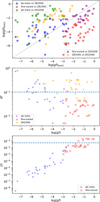 |
Fig. 4 Upper panel: comparison of theoretical log(gf) values for transitions with log(gf)RCI > −3.0 and Δlog(gf) > 1.0 dex shown in the left and middle panels of Figure 3. Middle panel: scatter plot of dT values. Lower panel: scatter plot of CF values. The dashed lines in the middle panel and the lower panel represent dT = 0.1 and CF = 0.05, respectively. ZB2006: Zatsarinny & Bartschat (2006); DH2008: Deb & Hibbert (2008). |
Comparison of experimental and theoretical weighted oscillator strength, log(gf), for S I.
Comparison of experimental and theoretical radiative lifetimes (in units of nanosecond) for S I.
3.3 Lifetimes
Comparing the calculated lifetimes with the precise measured values can also help to evaluate the overall accuracy of the calculated transition data. Figure 5 presents a comparison of our fine-tuned and ab initio lifetimes in Babushkin and Coulomb gauges, respectively (upper panel), as well as with the results from ZB2006 and DH2008 (lower panel). The ab initio and fine-tuned lifetimes agree very well with each other, except for the levels with #19, #20, #28, #29, #30, and #58 in Table A.1. These levels also exhibit significant discrepancies with the results from ZB2006 and DH2008. For levels with #19, #20, and #58, the large discrepancies between ab initio and fine-tuned lifetimes are due to changes in the mixing coefficients of the CSFs caused by fine-tuning. For example, a level with #58 of 3p3(4S)6p 5P1 has a percentage purity of 92% in the ab initio calculation, which is close to pure LSJ-coupling. In contrast, fine-tuning reduced the percentage purity to 84%, with increased mixing with 3p3(2D)4p 1P1 to 7%, which shortens the lifetime of 3p3(4S)6p 5P1. The lifetimes of the triplet states ![Mathematical equation: $\[3 \mathrm{s} 3 \mathrm{p}^{5}~{ }^{3} \mathrm{P}_{2,1,0}^{\mathrm{o}}\]$](/articles/aa/full_html/2026/03/aa57067-25/aa57067-25-eq35.png) (levels with #28, #29, and #30) are partly determined by the TEOP transitions 3s3p5 3Po–3s23p34p 3P, 5P and the IC transitions
(levels with #28, #29, and #30) are partly determined by the TEOP transitions 3s3p5 3Po–3s23p34p 3P, 5P and the IC transitions ![Mathematical equation: $\[3 \mathrm{s} 3 \mathrm{p}^{5}~{ }^{3} \mathrm{P}^{\mathrm{o}}{-}3 \mathrm{s}^{2} 3 \mathrm{p}^{4}~{ }^{1} \mathrm{D},{ }^{1} \mathrm{S}\]$](/articles/aa/full_html/2026/03/aa57067-25/aa57067-25-eq36.png) ; these transitions are driven by electron correlation and are very challenging to compute accurately. The triplet states are found to be strongly mixed with 3p3(2D)nd 3Po(n = 3 − 7). For these levels, the lifetimes in the Babushkin gauge are more stable, while fine-tuning causes larger changes in the Coulomb gauge. This is consistent with the results discussed in Section 3.2.3, which namely show that fine-tuning has a greater impact on the transition data in the Coulomb gauge.
; these transitions are driven by electron correlation and are very challenging to compute accurately. The triplet states are found to be strongly mixed with 3p3(2D)nd 3Po(n = 3 − 7). For these levels, the lifetimes in the Babushkin gauge are more stable, while fine-tuning causes larger changes in the Coulomb gauge. This is consistent with the results discussed in Section 3.2.3, which namely show that fine-tuning has a greater impact on the transition data in the Coulomb gauge.
Overall, the comparison in the lower panel of Figure 5 shows that our results have better agreement with those from ZB2006 than with DH2008. Among the 78 levels with three sets (ZB2006, DH2008 and our calculation) of lifetimes available, 69 of them show agreement with the results from ZB2006 within the range of 0.9 ≤ τ/τft ≤ 1.1, while only 35 levels from DH2008 meet this criterion. We also note that our computed lifetimes of the Rydberg states 3p3(4S)6d 5Do (levels with No. #97–#101) quintet and the 3p3(4S)7p 3P (levels with No. #102–#104) triplet also show significant differences from those of ZB2006. These levels also experience strong level mixing, especially the 3p3(4S)7p 3P triplet, which has a percentage purity of only about 50%. For ![Mathematical equation: $\[3 \mathrm{p}^{3}({ }^{4} \mathrm{S}) 6 \mathrm{d} ~5 \mathrm{D}_{4}^{\mathrm{o}}\]$](/articles/aa/full_html/2026/03/aa57067-25/aa57067-25-eq37.png) , our results, i.e. 266.27/269.21 ns from the ab initio calculation and 264.35/251.99 ns from the fine-tuned calculation, are in very good agreement with the experimental value of 260 ± 20 ns, which was obtained by Delalic et al. (1990) using the high-frequency deflection technique (see Table 3). In contrast, the results from ZB2006 are 165/163 ns, which are significantly lower than the experimental values.
, our results, i.e. 266.27/269.21 ns from the ab initio calculation and 264.35/251.99 ns from the fine-tuned calculation, are in very good agreement with the experimental value of 260 ± 20 ns, which was obtained by Delalic et al. (1990) using the high-frequency deflection technique (see Table 3). In contrast, the results from ZB2006 are 165/163 ns, which are significantly lower than the experimental values.
Table 3 compares our calculated lifetimes with other theoretical calculations and experimentally measured results. Other calculation results include B-spline calculation of ZB2006, HFR calculation of Biémont et al. (1998), CI calculation of DH2008, and MCHF calculation of Froese Fischer et al. (2006). In comparison to the others, the HFR results are generally much smaller, except for ![Mathematical equation: $\[3 \mathrm{p} 3({ }^{2} \mathrm{P}) 4 \mathrm{s}~^{3} \mathrm{P}_{0,1,2}^{\mathrm{o}}, 3 \mathrm{p}^{3}({ }^{2} \mathrm{D}) 4 \mathrm{p}~^{3} \mathrm{P}_{2}\]$](/articles/aa/full_html/2026/03/aa57067-25/aa57067-25-eq38.png) , and
, and ![Mathematical equation: $\[3 \mathrm{p}^{3}(^{4} \mathrm{S}) 6 \mathrm{d}~^{5} \mathrm{D}_{4}^{\mathrm{o}}\]$](/articles/aa/full_html/2026/03/aa57067-25/aa57067-25-eq39.png) . The theoretical results from the present calculations, as well as those from ZB2006 and DH2008, are in very good agreement with the experimental measurements obtained by Berzinsh et al. (1997) using laser spectroscopy and Beideck et al. (1994) using the beam-foil technique; they are also in good agreement with the astronomical observations by Federman & Cardelli (1995), except for the 3p3(4S)4d 3D1,2,3 states, where the lifetimes from DH2008 are approximately half of the measured results by Berzinsh et al. (1997). For the long-lived states, namely
. The theoretical results from the present calculations, as well as those from ZB2006 and DH2008, are in very good agreement with the experimental measurements obtained by Berzinsh et al. (1997) using laser spectroscopy and Beideck et al. (1994) using the beam-foil technique; they are also in good agreement with the astronomical observations by Federman & Cardelli (1995), except for the 3p3(4S)4d 3D1,2,3 states, where the lifetimes from DH2008 are approximately half of the measured results by Berzinsh et al. (1997). For the long-lived states, namely ![Mathematical equation: $\[3 \mathrm{p}^{3}({ }^{4} \mathrm{S}) 4 \mathrm{s}~^{5} \mathrm{S}_{2}^\mathrm{o}, 3 \mathrm{p}^{3}({ }^{4} \mathrm{S}) \mathrm{np}~^{5} \mathrm{P}_{3}(\mathrm{n}=5,6,7)\]$](/articles/aa/full_html/2026/03/aa57067-25/aa57067-25-eq40.png) , and
, and ![Mathematical equation: $\[3 \mathrm{p}^{3}({ }^{4}\mathrm{S}) 6 \mathrm{d}~^{3} \mathrm{D}_{2}^\mathrm{o}\]$](/articles/aa/full_html/2026/03/aa57067-25/aa57067-25-eq41.png) , there are significant differences between theoretical and experimental measurements, nor among different calculations and experimental results. For these energy levels, which are dominated by weak transitions, both theoretical calculations and experimental measurements are challenging. In addition, the measurements of lifetimes for long-lived states often have large uncertainties and further precise measurements are needed.
, there are significant differences between theoretical and experimental measurements, nor among different calculations and experimental results. For these energy levels, which are dominated by weak transitions, both theoretical calculations and experimental measurements are challenging. In addition, the measurements of lifetimes for long-lived states often have large uncertainties and further precise measurements are needed.
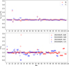 |
Fig. 5 Upper: comparison of fine-tuned lifetimes (ft) between Babushkin (B) and Coulomb (C) gauges. Lower: comparison of fine-tuned lifetimes with other theoretical results. ZB2006: Zatsarinny & Bartschat (2006); DH2008 Deb & Hibbert (2008). ZB2006/ft, B/B: the Babushkin gauge of ZB2006 divided by the Babushkin gauge of fine-tuned lifetimes. The three dashed grey lines represent τ/τft = 0.9, 1.0, and 1.1, respectively. |
4 Conclusion
The energy levels, transition data, and lifetimes of S I were calculated using both the ab initio and fine-tuning approaches based on the MCDHF and RCI methods. We found that fine-tuning provides more accurate mixing coefficients, which correctly position the energy levels. It can also better improve the results in the Coulomb gauge, which is typically less accurate in ab initio calculations. The corrections to the wave functions resulting from fine-tuning improve the consistency of the transition data between the Babushkin and Coulomb gauges, thereby enhancing the accuracy of the transition data.
We conducted extensive comparisons with various theoretical and experimental results. The accuracy level of the computed data was evaluated using a combination of gauge differences parameters and CFs. For applications requiring complete atomic datasets, we recommend using the fine-tuned data in the Babushkin gauge; for specific transitions, cross-validation with different sources is advised to ensure reliability. Notably, significant discrepancies were observed among different theoretical calculations for certain transitions, particularly for the solar-abundance diagnostic lines. The lack of precise experimental measurements complicates the assessment of the accuracy of different calculations. Further experimental efforts are essential to validating and constraining theoretical predictions.
The atomic data provided in this study can be used for astrophysical applications, not least non-LTE stellar spectroscopic analyses (e.g. Korotin & Kiselev 2024). In particular, the implications of these new data on the solar sulphur abundance were recently discussed in detail in Amarsi et al. (2025).
Data availability
The full versions of Table A.1 and Table A.2 are available at the CDS via https://cdsarc.cds.unistra.fr/viz-bin/cat/J/A+A/707/A141.
Acknowledgements
WL acknowledges the support from the National Key R&D Program of China No. 2022YFF0503800, the National Natural Science Foundation of China (NSFC, Grant No. 12373058) and the specialized research fund for State Key Laboratory of Solar Activity and Space Weather. AMA acknowledges support from the Swedish Research Council (VR 2020-03940) the Crafoord Foundation via the Royal Swedish Academy of Sciences (CR 2024-0015), and the European Union’s Horizon Europe research and innovation programme under grant agreement No. 101079231 (EXOHOST). PJ acknowledges support from the Swedish Research Council (VR 2023-05367). AMA and WL also acknowledge support from the 2024 Chinese Academy of Sciences (CAS) President’s International Fellowship Initiative (PIFI). WL thanks Yanting Li for the helpful discussion with the rfinetune code. We would also like to thank the anonymous referee for providing useful comments that helped improve the original manuscript.
References
- Amarsi, A. M., Li, W., Grevesse, N., & Jurewicz, A. J. G. 2025, A&A, 703, A35 [NASA ADS] [CrossRef] [EDP Sciences] [Google Scholar]
- Anderson, D. E., Bergin, E. A., Maret, S., & Wakelam, V. 2013, ApJ, 779, 141 [Google Scholar]
- Beideck, D. J., Schectman, R. M., Federman, S. R., & Ellis, D. G. 1994, ApJ, 428, 393 [Google Scholar]
- Berzinsh, U., Caiyan, L., Zerne, R., Svanberg, S., & Biémont, E. 1997, Phys. Rev. A, 55, 1836 [Google Scholar]
- Biémont, E., Storey, P. J., & Zeippen, C. J. 1996, A&A, 309, 991 [Google Scholar]
- Biémont, E., Garnir, H. P., Federman, S. R., Li, Z. S., & Svanberg, S. 1998, ApJ, 502, 1010 [Google Scholar]
- Bridges, J. M., & Wiese, W. L. 1967, Phys. Rev., 159, 31 [Google Scholar]
- Caffau, E., Faraggiana, R., Bonifacio, P., Ludwig, H.-G., & Steffen, M. 2007, A&A, 470, 699 [NASA ADS] [CrossRef] [EDP Sciences] [Google Scholar]
- Carpenter, K. G., Robinson, R. D., Wahlgren, G. M., Linsky, J. L., & Brown, A. 1994, ApJ, 428, 329 [Google Scholar]
- Chen, Z., & Msezane, A. Z. 1997, J. Phys. B At. Mol. Phys., 30, 3873 [Google Scholar]
- Chen, M. H., Cheng, K. T., & Johnson, W. R. 2001, Phys. Rev. A, 64, 042507 [Google Scholar]
- Civiš, S., Kramida, A., Zanozina, E. M., et al. 2024, ApJS, 274, 32 [Google Scholar]
- Corrégé, G., & Hibbert, A. 2004, At. Data Nucl. Data Tables, 86, 19 [Google Scholar]
- Costa Silva, A. R., Delgado Mena, E., & Tsantaki, M. 2020, A&A, 634, A136 [EDP Sciences] [Google Scholar]
- Cowan, R. D. 1981, The Theory of Atomic Structure and Spectra, 1st edn., 3 (University of California Press) [Google Scholar]
- da Silva, R., D’Orazi, V., Palla, M., et al. 2023, A&A, 678, A195 [NASA ADS] [CrossRef] [EDP Sciences] [Google Scholar]
- Daflon, S., Cunha, K., Smith, V. V., & Butler, K. 2003, A&A, 399, 525 [NASA ADS] [CrossRef] [EDP Sciences] [Google Scholar]
- Deb, N. C., & Hibbert, A. 2006, J. Phys. B At. Mol. Phys., 39, 4301 [Google Scholar]
- Deb, N. C., & Hibbert, A. 2008, At. Data Nucl. Data Tables, 94, 561 [Google Scholar]
- Delalic, Z., Erman, P., & Kallne, E. 1990, Phys. Scr, 42, 540 [Google Scholar]
- Doering, J. P. 1990, J. Geophys. Res., 95, 21313 [Google Scholar]
- Duffau, S., Caffau, E., Sbordone, L., et al. 2017, A&A, 604, A128 [NASA ADS] [CrossRef] [EDP Sciences] [Google Scholar]
- Durrance, S. T., Feldman, P. D., & Weaver, H. A. 1983, ApJ, 267, L125 [Google Scholar]
- Dyall, K., Grant, I., Johnson, C., Parpia, F., & Plummer, E. 1989, Comput. Phys. Commun., 55, 425 [NASA ADS] [CrossRef] [Google Scholar]
- Ekman, J., Godefroid, M., & Hartman, H. 2014, Atoms, 2, 215 [CrossRef] [Google Scholar]
- Fawcett, B. C. 1986, At. Data Nucl. Data Tables, 35, 185 [Google Scholar]
- Feaga, L. M., McGrath, M. A., & Feldman, P. D. 2002, ApJ, 570, 439 [Google Scholar]
- Federman, S. R., & Cardelli, J. A. 1995, ApJ, 452, 269 [Google Scholar]
- Federman, S. R., & Cardelli, J. A. 1996, Phys. Scr., 1996, 158 [Google Scholar]
- Fischer, C. F. 1987, J. Phys. B: At. Mol. Phys., 20, 4365 [Google Scholar]
- Fleming, J., & Hibbert, A. 1999, Phys. Scr. Vol. T, 83, 44 [Google Scholar]
- Froese Fischer, C. 2009, Phys. Scr. Vol. T, 134, 014019 [Google Scholar]
- Froese Fischer, C., & Tachiev, G. 2004, At. Data Nucl. Data Tables, 87, 1 [NASA ADS] [CrossRef] [Google Scholar]
- Froese Fischer, C., Tachiev, G., & Irimia, A. 2006, At. Data Nucl. Data Tables, 92, 607 [NASA ADS] [CrossRef] [Google Scholar]
- Froese Fischer, C., Tachiev, G., Gaigalas, G., & Godefroid, M. R. 2007, Comput. Phys. Commun., 176, 559 [NASA ADS] [CrossRef] [Google Scholar]
- Froese Fischer, C., Godefroid, M., Brage, T., Jönsson, P., & Gaigalas, G. 2016, J. Phys. B: At. Mol. Opt. Phys., 49, 182004 [CrossRef] [Google Scholar]
- Froese Fischer, C., Gaigalas, G., Jönsson, P., & Bieroń, J. 2019, Comput. Phys. Commun., 237, 184 [NASA ADS] [CrossRef] [Google Scholar]
- Gaigalas, G., Rudzikas, Z., & Froese Fischer, C. 1997, J. Phys. B At. Mol. Phys., 30, 3747 [Google Scholar]
- Gaigalas, G., Fritzsche, S., & Grant, I. P. 2001, Comput. Phys. Commun., 139, 263 [NASA ADS] [CrossRef] [Google Scholar]
- Gaigalas, G., Žalandauskas, T., & Rudzikas, Z. 2003, At. Data Nucl. Data Tables, 84, 99 [Google Scholar]
- Gaigalas, G., Zalandauskas, T., & Fritzsche, S. 2004, Comput. Phys. Commun., 157, 239 [Google Scholar]
- Gaigalas, G., Froese Fischer, C., Rynkun, P., & Jönsson, P. 2017, Atoms, 5, 6 [CrossRef] [Google Scholar]
- Gaigalas, G., Rynkun, P., Radžiūtė, L., et al. 2020, ApJS, 248, 13 [CrossRef] [Google Scholar]
- Gaigalas, G., Rynkun, P., Domoto, N., et al. 2024, MNRAS, 530, 5220 [Google Scholar]
- Ganas, P. S. 1982, Phys. Lett. A, 87, 394 [Google Scholar]
- Grant, I. P. 1974, J. Phys. B At. Mol. Phys., 7, 1458 [Google Scholar]
- Grant, I. P. 2007, Relativistic Quantum Theory of Atoms and Molecules (New York: Springer) [Google Scholar]
- Hibbert, A. 1974, J. Phys. B: At. Mol. Phys., 7, 1417 [NASA ADS] [CrossRef] [Google Scholar]
- Hibbert, A. 1975, Comput. Phys. Commun., 9, 141 [Google Scholar]
- Ho, Y. K., & Henry, R. J. W. 1985, ApJ, 290, 424 [Google Scholar]
- Judge, P. G. 1988, MNRAS, 231, 419 [Google Scholar]
- Jönsson, P., Gaigalas, G., Fischer, C. F., et al. 2023a, Atoms, 11 [Google Scholar]
- Jönsson, P., Godefroid, M., Gaigalas, G., et al. 2023b, Atoms, 11 [Google Scholar]
- Kamp, I., Iliev, I. K., Paunzen, E., et al. 2001, A&A, 375, 899 [NASA ADS] [CrossRef] [EDP Sciences] [Google Scholar]
- Kaufman, V., & Martin, W. C. 1993, J. Phys. Chem. Ref. Data, 22, 279 [Google Scholar]
- Korotin, S. A., & Kiselev, K. O. 2024, Astron. Rep., 68, 1159 [Google Scholar]
- Kramida, A., Yu. Ralchenko, Reader, J., & NIST ASD Team 2024, NIST Atomic Spectra Database (ver. 5.12), [Online]. Available: https://physics.nist.gov/asd [2025, August 21]. National Institute of Standards and Technology, Gaithersburg, MD [Google Scholar]
- Kurucz, R. L., & Peytremann, E. 1975, SAO Special Report [Google Scholar]
- Laverick, M., Lobel, A., Royer, P., et al. 2019, A&A, 624, A60 [NASA ADS] [CrossRef] [EDP Sciences] [Google Scholar]
- Li, M. C., Li, W., Jönsson, P., Amarsi, A. M., & Grumer, J. 2023a, ApJS, 265, 26 [NASA ADS] [CrossRef] [Google Scholar]
- Li, W., Jönsson, P., Amarsi, A. M., Li, M. C., & Grumer, J. 2023b, A&A, 674, A54 [NASA ADS] [CrossRef] [EDP Sciences] [Google Scholar]
- Li, Y., Gaigalas, G., Li, W., Chen, C., & Jönsson, P. 2023, Atoms, 11 [Google Scholar]
- Lundberg, H., Li, Z. S., & Jönsson, P. 2001, Phys. Rev. A, 63, 032505 [Google Scholar]
- Mason, N. J. 1994, Phys. Scr., 49, 578 [Google Scholar]
- Müller, D. 1968, Zeitsch. Naturf. A, 23, 1707 [Google Scholar]
- Nissen, P. E., Akerman, C., Asplund, M., et al. 2007, A&A, 469, 319 [NASA ADS] [CrossRef] [EDP Sciences] [Google Scholar]
- Olsen, J., Roos, B. O., Jo/rgensen, P., & Jensen, H. J. A. 1988, J. Chem. Phys., 89, 2185 [NASA ADS] [CrossRef] [Google Scholar]
- Papoulia, A., Ekman, J., Gaigalas, G., et al. 2019, Atoms, 7, 106 [NASA ADS] [CrossRef] [Google Scholar]
- Papoulia, A., Ekman, J., & Jönsson, P. 2019, A&A, 621, A16 [NASA ADS] [CrossRef] [EDP Sciences] [Google Scholar]
- Podobedova, L. I., Kelleher, D. E., & Wiese, W. L. 2009, J. Phys. Chem. Ref. Data, 38, 171 [NASA ADS] [CrossRef] [Google Scholar]
- Savage, B. D., & Lawrence, G. M. 1966, ApJ, 146, 940 [NASA ADS] [CrossRef] [Google Scholar]
- Scott, P., Grevesse, N., Asplund, M., et al. 2015, A&A, 573, A25 [NASA ADS] [CrossRef] [EDP Sciences] [Google Scholar]
- Skillman, E. D., & Kennicutt, Jr., R. C. 1993, ApJ, 411, 655 [NASA ADS] [CrossRef] [Google Scholar]
- Skúladóttir, Á., Andrievsky, S. M., Tolstoy, E., et al. 2015, A&A, 580, A129 [NASA ADS] [CrossRef] [EDP Sciences] [Google Scholar]
- Starace, A. F. 1971, Phys. Rev. A, 3, 1242 [Google Scholar]
- Sturesson, L., Jönsson, P., & Froese Fischer, C. 2007, Comput. Phys. Commun., 177, 539 [NASA ADS] [CrossRef] [Google Scholar]
- Takeda, Y., Hashimoto, O., Taguchi, H., et al. 2005, PASJ, 57, 751 [NASA ADS] [Google Scholar]
- Tayal, S. S. 1998, ApJ, 497, 493 [Google Scholar]
- Tennyson, J. 2019, Astronomical Spectroscopy. An Introduction to the Atomic and Molecular Physics of Astronomical Spectroscopy (World Scientific) [Google Scholar]
- Zatsarinny, O., & Bartschat, K. 2006, J. Phys. B At. Mol. Phys., 39, 2861 [Google Scholar]
- Zerne, R., Caiyan, L., Berzinsh, U., & Svanberg, S. 1997, Phys. Scr., 56, 459 [NASA ADS] [CrossRef] [Google Scholar]
- Zhang, W., Palmeri, P., Quinet, P., & Biémont, É. 2013, A&A, 551, A136 [NASA ADS] [CrossRef] [EDP Sciences] [Google Scholar]
GRASP is fully open source and is available on GitHub repository at https://github.com/compas/grasp maintained by the CompAS collaboration.
Note that some log(gf) values for S I transitions in NIST ASD are anomalous (Alexander Kramida, priv. commun.), while the line strength, S, and oscillator strength, f, values are correct. The log(gf) values from NIST ASD adopted in this paper were all calculated from the f values.
Appendix A Energy levels and transition data
Energy levels and lifetimes from ab initio and fine–tuning calculations.
Computed transition data.
All Tables
Comparison of experimental and theoretical weighted oscillator strength, log(gf), for S I.
Comparison of experimental and theoretical radiative lifetimes (in units of nanosecond) for S I.
All Figures
|
Fig. 1 Energy differences as a function of excitation energies provided by NIST ASD. The dashed black and red lines are the linear fit to the data from ab initio (black plus) and fine-tuning (red plus) calculations, respectively. The inset in the upper right shows an enlarged view for ENIST > 5 × 104 cm−1. |
| In the text | |
|
Fig. 2 Left: comparison of log(gf) between Babushkin and Coulomb gauges for ab initio (black plus) and fine-tuned (red plus) results, respectively. Insets (a1) and (a2) show the histograms of the log(gf) differences for transitions with log(gf) ≥ −2 and log(gf) < −2, respectively. Right: comparison of log(gf) between ab initio and fine-tuned calculations for Babushkin (black diamond) and Coulomb gauges (red hexagon), respectively. Insets (b1) and (b2) show the histograms of the log(gf) differences for transitions with log(gf) ≥ −3 and log(gf) < −3, respectively. |
| In the text | |
|
Fig. 3 Comparison of log(gf) from the current study with those from previous works. Left: ZB2006 (Zatsarinny & Bartschat 2006). Middle: DH2008 (Deb & Hibbert 2008). Right: NIST ASD (Kramida et al. 2024). The data in NIST ASD were compiled from various sources, including Müller (1968); Beideck et al. (1994); Biémont et al. (1996, 1998); Zerne et al. (1997); Froese Fischer et al. (2006) and Zatsarinny & Bartschat (2006). Babushkin results from present ab initio (black plus) and fine-tuned (red plus) RCI calculations are used in the comparison. The inset figures show the histograms of the distribution of the number of transitions for the differences in log(gf). Note that the y-axis range is consistent across all plots in Figures 2 and 3. |
| In the text | |
|
Fig. 4 Upper panel: comparison of theoretical log(gf) values for transitions with log(gf)RCI > −3.0 and Δlog(gf) > 1.0 dex shown in the left and middle panels of Figure 3. Middle panel: scatter plot of dT values. Lower panel: scatter plot of CF values. The dashed lines in the middle panel and the lower panel represent dT = 0.1 and CF = 0.05, respectively. ZB2006: Zatsarinny & Bartschat (2006); DH2008: Deb & Hibbert (2008). |
| In the text | |
|
Fig. 5 Upper: comparison of fine-tuned lifetimes (ft) between Babushkin (B) and Coulomb (C) gauges. Lower: comparison of fine-tuned lifetimes with other theoretical results. ZB2006: Zatsarinny & Bartschat (2006); DH2008 Deb & Hibbert (2008). ZB2006/ft, B/B: the Babushkin gauge of ZB2006 divided by the Babushkin gauge of fine-tuned lifetimes. The three dashed grey lines represent τ/τft = 0.9, 1.0, and 1.1, respectively. |
| In the text | |
Current usage metrics show cumulative count of Article Views (full-text article views including HTML views, PDF and ePub downloads, according to the available data) and Abstracts Views on Vision4Press platform.
Data correspond to usage on the plateform after 2015. The current usage metrics is available 48-96 hours after online publication and is updated daily on week days.
Initial download of the metrics may take a while.