| Issue |
A&A
Volume 707, March 2026
|
|
|---|---|---|
| Article Number | A201 | |
| Number of page(s) | 13 | |
| Section | Interstellar and circumstellar matter | |
| DOI | https://doi.org/10.1051/0004-6361/202557653 | |
| Published online | 12 March 2026 | |
Polycyclic aromatic hydrocarbon spectral diversity in NGC 7027 and the evolution of aromatic carriers
1
Department of Physics & Astronomy, The University of Western Ontario,
London,
ON
N6A 3K7,
Canada
2
Institute for Earth and Space Exploration, The University of Western Ontario,
London,
ON
N6A 3K7,
Canada
3
Leiden Observatory, Leiden University,
PO Box 9513,
2300
RA
Leiden,
The Netherlands
4
Astronomy Department, University of Maryland,
College Park,
MD
20742,
USA
5
NASA Ames Research Center,
MS 245-6,
Moffett Field,
CA
94035-1000,
USA
6
Carl Sagan Center, SETI Institute,
339 Bernardo Avenue, Suite 200,
Mountain View,
CA
94043,
USA
★ Corresponding author: This email address is being protected from spambots. You need JavaScript enabled to view it.
Received:
10
October
2025
Accepted:
15
January
2026
Abstract
Context. Polycyclic aromatic hydrocarbons (PAHs) constitute a significant fraction of the Universe’s carbon budget, playing a key role in the cosmic carbon cycle and dominating the mid-infrared spectra of astrophysical environments in which they reside. Although PAHs are known to form in the circumstellar envelopes of post-asymptotic giant branch stars, their formation and evolution are still not well understood.
Aims. We aim to understand how pristine complex hydrocarbons and PAHs in circumstellar environments transition to the PAHs observed in the interstellar medium.
Methods. The mid-infrared PAH spectra (5–18 μm) of the planetary nebula, NGC 7027, were investigated using spectral cubes from JWST MIRI-MRS.
Results. We report the first detection of spatially resolved variations of the PAH spectral profiles across class 𝒜, 𝒜ℬ, and ℬ in all major PAH bands (6.2, 7.7, 8.6, and 11.2 μm) within a single source, NGC 7027. These variations are linked to morphological structures within NGC 7027. Clear correlations are revealed between the 6.2, 7.7, and 8.6 μm features, where the red components (6.26, 7.8, and 8.65 μm) exhibit a strong correlation and the same is found for the blue components of the 6.2 and 7.7 μm features (6.205 and 7.6 μm). The blue component of the 8.6 μm feature (8.56 μm) appears to be independent of the other components. We link this behavior to differences in the molecular structure of their PAH subpopulations. Decomposition of the 11.2 μm band confirms two previously identified components, with the broader 11.25 μm component attributed to emission from very small grains or PAH clusters rather than PAH emission.
Conclusions. We show that PAH profile classes generally vary with proximity to the central star’s UV radiation field, suggesting class ℬ PAHs represent more processed species while class 𝒜 PAHs remain relatively pristine, challenging current notions on the spectral evolution of PAHs.
Key words: techniques: spectroscopic / circumstellar matter / ISM: molecules / planetary nebulae: individual: NGC 7027
© The Authors 2026
 Open Access article, published by EDP Sciences, under the terms of the Creative Commons Attribution License (https://creativecommons.org/licenses/by/4.0), which permits unrestricted use, distribution, and reproduction in any medium, provided the original work is properly cited.
This article is published in open access under the Subscribe to Open model. This email address is being protected from spambots. You need JavaScript enabled to view it. to support open access publication.
1 Introduction
The outflows of dying intermediate-mass stars – i.e., asymptotic giant branch (AGB) stars – are the birth site for dust and carbon-related species, such as polycyclic aromatic hydrocarbons (PAHs; e.g., Frenklach & Feigelson 1989; Boersma et al. 2006; Galliano et al. 2008a; Tielens 2008). Carbon-rich AGB stars dictate the early chemistry in their circumstellar envelopes before the molecules and dust are later incorporated into the interstellar medium (ISM), providing the main source of carbon and other organic elements for the ISM (e.g., Cherchneff et al. 1992; Tielens 2005; Matsuura et al. 2009). Therefore, PAH emission from post-AGB stars and planetary nebulae (PNe) can be studied to unveil the PAH characteristics at the beginning stages of their life cycle.
The characteristics of the PAH population are strongly influenced by the temperature, density, and radiation field of the environment in which they reside. It follows that the PAH emission bands reflect the conditions of their environment, and spectral variations arise in the form of relative intensity, peak emission position, and profile shape (e.g., Cohen et al. 1986; Smith et al. 2007; Galliano et al. 2008b).
Based on observed peak positions and profile shapes of the 3.3, 6.2, 7.7, and 11.2 μm aromatic infrared bands (AIBs), spectra can be categorized into different classes: 𝒜 −𝒟 (Peeters et al. 2002; van Diedenhoven et al. 2004; Matsuura et al. 2014; Sloan et al. 2014). These different AIB classes correlate with the source type (i.e., H II regions, reflection nebulae, Herbig AeBe stars, planetary nebulae; Cohen et al. 1989; Bregman et al. 1989; Peeters et al. 2002; van Diedenhoven et al. 2004) and the observed spectral differences are thought to reflect processing of the PAHs in the local environment by prevalent far-ultraviolet (FUV) photons, shocks, and/or gas phase chemistry (e.g., Peeters et al. 2002; Boersma et al. 2008; Matsuura et al. 2014). Likely, there is an evolutionary relationship between these classes. It has indeed been suggested that recently formed PAHs are predominantly class ℬ ones, but processing in the harsh environment of the ISM converts them into class 𝒜 PAHs (e.g., Peeters et al. 2002; Boersma et al. 2008; Matsuura et al. 2014). A somewhat different scenario is envisioned by Joblin et al. (2008) in which PAHs that formed in C-rich AGB outflows are rich in aliphatics and these species are converted into highly aromatic compounds in harsh radiation fields. There is observational evidence that this conversion already occurs in the (proto)-planetary nebula phase (Goto et al. 2003, 2007).
Infrared studies with the Infrared Space Observatory Short Wavelength Spectrometer (ISO-SWS) have revealed that the planetary nebula, NGC 7027, has an AIB spectrum that is a mix of class 𝒜 and ℬ (Peeters et al. 2002; van Diedenhoven et al. 2004). This source therefore provides a unique opportunity to assess the factors that drive the conversion from class ℬ to class 𝒜. However, the beam size of the SWS instrument was similar to the size of this source in the mid-IR and thus precluded a detailed study of the spatial distribution of the AIBs to trace this evolution in the outflow. The Mid-Infrared Instrument Integral Field Unit (MIRI IFU; Wright et al. 2015; Wells et al. 2015) on board the James Webb Space Telescope (JWST; Gardner et al. 2006) with a pixel scale of 0.2” is well suited to study the spatial-spectral distribution of the AIBs in this nebula.
In Section 2, we describe the AIB classification and, in Section 3, we discuss the morphology of NGC 7027. Details about the observations, data reduction, and analysis are discussed in Section 4. We present the results in Section 5, followed by a discussion in Section 6. Finally, the conclusions of the study are laid out in Section 7.
2 AIB classification
Class 𝒜 profiles exhibit the bluest peak positions. For class 𝒜 profiles, the 6.2 μm band has a peak position between 6.19 and 6.23 μm, the 7.6 μm feature is the dominant component of the 7.7 μm complex, and the 8.6 μm feature peaks between 8.58 and 8.62 μm (Peeters et al. 2002). For the 11.2 μm band, a class 𝒜 or 𝒜ℬ profile peaks at 11.20–11.24 μm. The difference between the 11.2 μm 𝒜 and 𝒜ℬ classifications arises from the full width at half maximum (FWHM), where a class 𝒜 profile has a narrower profile than that of class 𝒜ℬ (van Diedenhoven et al. 2004). Class ℬ, on the other hand, demonstrates redshifted peak positions. In this case, the 7.8 μm component is the dominant one of the 7.7 μm complex and the 8.6 μm feature peaks at a wavelength longward of 8.62 μm. Meanwhile, the 6.2 μm feature peaks between 6.24 and 6.28 μm, and the 11.2 μm band is relatively broad with a peak at ~11.25 μm. In class 𝒞 spectra, the 6.2 μm feature peaks at 6.29 μm and the 7–9 μm complex has a very broad band peaking around 8.2 μm (Peeters et al. 2017). Finally, class 𝒟 has been assigned to PAH spectra with a broad feature peaking at 6.24 μm, a broad feature ranging from 7–9 μm peaking at 7.7 μm, and a peak position at ~11.4 μm of the 11.2 μm PAH band (Matsuura et al. 2014; Sloan et al. 2014). It is important to note that PAH spectra do not simply fall into a discrete class but, rather, seem to form a continuous distribution ranging from Class 𝒜 to 𝒟.
Observations demonstrate that each class has a connection to the astronomical object in which they are observed. Class 𝒜 band profiles are attributed to interstellar material, typically being observed in reflection nebulae, the ISM, and H II regions. Class ℬ and 𝒞 are associated with circumstellar material, being most commonly detected in post-AGB stars, planetary nebulae, and isolated Herbig AeBe stars (e.g., Cohen et al. 1989; Bregman et al. 1989; Peeters et al. 2002; Tielens 2008).
Fig. 1 shows the MIRI medium-resolution spectrometer (MRS) integrated spectrum of NGC 7027 along with archetypal spectra for PAH profile classes 𝒜 and ℬ for each of the 6.2, 7.7, 8.6, and 11.2 μm features. The MIRI integrated spectrum shows a mix of PAH profile classes. The 6.2 and 8.6 μm PAH profiles exhibit a class 𝒜 profile whereas the 7.7 and 11.2 μm features show a class 𝒜ℬ profile.
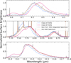 |
Fig. 1 MIRI-MRS integrated spectrum of NGC 7027 along with the PAH profile class 𝒜 (blue) and ℬ (red) for the 6.2, 7–9, and 11.2 μm features (exemplified by IRAS 23133+6050 and HD 44179 respectively; taken from Peeters et al. 2002; van Diedenhoven et al. 2004). |
3 NGC 7027
NGC 7027 is a relatively nearby (~900 pc) carbon-rich PN (Masson 1989; Zijlstra et al. 2008). At a young dynamical age of roughly 600 years, it is still at a relatively early stage of the PN phase of stellar evolution (Masson 1989). NGC 7027 is very bright; at its center lies a very hot white dwarf (WD) with an effective temperature of about 200 000 K and a luminosity of roughly 8000 L⊙ (Latter et al. 2000; Zhang et al. 2005). The current core mass is estimated to be ~0.65 M⊙ (Zijlstra et al. 2008), while the progenitor mass is estimated to have been 3–4 M⊙ (Bernard Salas et al. 2001).
Numerous infrared and submillimeter observations have revealed that the material ejected during the AGB phase has formed a flattened ellipsoidal distribution (Fig. 3; Cox et al. 2002). This nonspherical distribution is likely due to the presence of a binary system at the center of the nebula, as many studies of PNe suggest (e.g., Balick & Frank 2002; De Marco 2009; Moraga Baez et al. 2023). Strong, precessing jets have carved out bipolar cones that are being illuminated by the extreme-ultraviolet (EUV) and FUV photons from the hot central white dwarf (Latter et al. 2000; Cox et al. 2002). These conditions create an ionized nebula, which forms a dense, clumpy, and limb-brightened elliptical ring (Cox et al. 2002; Tielens 2005), an adjacent photodissociation region (PDR), and a surrounding molecular cloud, all expanding with a typical velocity of ~20 km s−1 (Cox et al. 1997; Latter et al. 2000; Bublitz et al. 2023). A simplified schematic of NGC 7027 as viewed from the side is shown in Fig. 2.
The H2 morphology is remarkably different from the morphology of the ionized gas. The H2 emission shows a four-lobed structure that is formed by a limb-brightened biconical shell (Fig. 3; Graham et al. 1993; Kastner et al. 1994). This hourglass-like shell is thought to be capped at both ends, producing the limb brightening observed in the outer rims of the bicone (Latter et al. 2000). The kinematics of the H2 distribution reveal that the lower cone faces toward the line of sight and has an inclination angle of i ~ 60° and the upper cone faces away from the observer (Cox et al. 2002). There is enhanced H2 emission in the equatorial waist due to limb brightening of the inner rims of the biconical shell (Latter et al. 2000; Cox et al. 2002). The asymmetry observed in the lobes is due to the presence of three bipolar outflows that, over time, have carved out holes in the H2 distribution, the most pronounced being “Outflow 1” at a position angle of −53° (Cox et al. 2002; Nakashima et al. 2010). Appendix A details the H2, ionized gas, and 6.2 μm PAH emission as observed by JWST MIRI-MRS within the channel 1 field of view (CH1 FOV; Fig. A.1). The edges of the elliptical ring are pictured by the ionized gas and the 6.2 μm PAH emission (which sits just outside the H II region in the PDR), while the equatorial waist is delineated by the H2 emission. The nebula seems to exhibit the typical layered PDR structure.
The CO emission, which traces the cold, dense material surrounding the PDR, sits further outside the H2 emission and displays a roughly elliptical morphology with particularly bright edges in the NE and SW (Bublitz et al. 2023). Narrow dust lanes are observed along the equatorial belt, and nonuniform dust filaments are observed surrounding the lobed and elliptical ring structures, most prominently around the NE lobe (Kastner et al. 2020; Moraga Baez et al. 2023). Outflow-driven shocks play an important role in the processing of ejected material and are thought to be a mechanism for very small grain and PAH formation in the PN via grain-grain collisions (Lau et al. 2016).
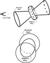 |
Fig. 2 Simplified schematic drawings of NGC 7027 as viewed from the side (top) and the front (bottom). The central star in shown in yellow. The H2 emission primarily lies on the surface of the biconical shell, and is particularly bright along the rims, while the ionized gas and PAHs reside within the elliptical ring. |
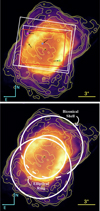 |
Fig. 3 Top: HST/WFC3 NICMOS F212N image of NGC 7027 with JWST MIRI-MRS FOVs for channels 1 (red), 2, and 3 (white) overlaid. The black cross indicates the position of the central star. The yellow contours outline the H2 gas morphology in the continuum-subtracted HST/NICMOS images from Latter et al. (2000). The small orange, pink, blue, and green boxes are the spaxels used to illustrate the AIB variability referred to hereinafter as the E ring, outer NE corner, inner region, and the SW ring, respectively. Bottom: HST/WFC3 NICMOS F212N image of NGC 7027 with a schematic drawing overlaid. Credit: NASA/ESA, Latter et al. (2000). |
4 Observations, data reduction and analysis
We present JWST MIRI-MRS IFU (Wright et al. 2015; Wells et al. 2015; Wright et al. 2023; Argyriou et al. 2023) observations of NGC 7027 (program ID 01523, observation 1). A 3 × 3 mosaic was taken centered on the central star. The resulting spectral cubes cover a wavelength range of 4.9–27.9 μm at a spectral resolution of R ~ 1500–3500 over a FOV of up to 9.8″ × 8.5″ depending on the channel (Fig. 3).
We reduced the data using the JWST science calibration pipeline version 1.15.1 and the CRDS reference file context 1293. We used the default pipeline settings with the exception of performing a residual fringe correction in stage 2 of the pipeline and setting the output cube types to subchannels.
We used data from channels 1 to 3 (4.9–18 μm). For comparative analysis, we used the pixel size of channel 3 (0.2″ × 0.2″) and the FOV of the channel 1 mosaic (7.5″ × 6″). We performed multiplicative stitching between subchannels to obtain the final spectra. We analyzed individual spaxels and extracted a spectrum across the channel 1 FOV, further referred to as the MIRI-MRS integrated spectrum (see Table B.1 for details).
We determined the dust continuum to extract the profiles of the 6.2, 7.7–8.6, and 11.2 μm PAHs (see Appendix C for details) and classify their profiles based on the classification of Peeters et al. (2002) and van Diedenhoven et al. (2004). To facilitate the discussion, we employed four spectra extracted in the apertures shown in Fig. 3 (see Table B.1), probing the NE corner – outside the elliptical ring (pink), the E side of the elliptical ring (orange), the central region (blue), and the SW portion of the elliptical ring (green).
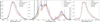 |
Fig. 4 Illustration of the 6.2, 7–9, and 11.2 μm profile variation across the nebula. The single spaxel spectra from Fig. 3 detailed in Table B.1 are utilized here. |
5 Results
Overall, the PAH emission in the MIRI-MRS integrated spectrum (see Fig. 1) of NGC 7027 resembles those reported in the literature (e.g., ISO-SWS; Peeters et al. 2002; van Diedenhoven et al. 2004). However, due to the distinct extraction apertures (7.5″ × 6″ for MIRI-MRS versus 14″ × 20″ for ISO-SWS), differences emerge upon close inspection of the spectral profiles (Fig. 4, Table D.1). The MIRI data reveal that the PAH emission varies systematically across the nebula.
5.1 Spatial variation of the PAH spectral profiles
The spaxel spectra demonstrate wide PAH profile variation across NGC 7027 in each of the major features observed (Fig. 4). We investigated the profile class of the 6.2, 7.7, 8.6, and 11.2 μm PAH bands.
The spatial variations in PAH profile classes reveal a striking morphological pattern across NGC 7027. In the 6.2 μm feature, the outer NE corner of the CH1 FOV (beyond the elliptical ring) is dominated by a strong class 𝒜 profile, with a narrow profile peaking at 6.205 μm (Fig. 5). Within the ring, however, this shifts to a clear class ℬ profile that is broader in shape and peaks at 6.24 μm. The central region presents an intermediate case: while the peak remains consistent with class 𝒜, the band is noticeably broader than in the NE corner.
A similar progression is observed in the 7.7 μm feature. In the NE corner, a class 𝒜 profile is evident, where the 7.6 μm component dominates over the 7.8 μm band (Fig. 5). In contrast, the ring exhibits a pure class ℬ profile with a strong 7.8 μm peak, while the inner region contains a mixture of intermediate class 𝒜ℬ and class ℬ profiles.
The 8.6 μm feature follows the same spatial trend. A class 𝒜 profile with a peak at ~8.6 μm is found in the NE corner, transitioning to a class ℬ profile at ~8.65 μm within the ring, and reverting to class 𝒜 profiles in the inner region.
Finally, the 11.2 μm feature echoes this pattern. The NE corner again shows a class 𝒜 profile at 11.2 μm, while the ring hosts class ℬ profiles. The inner region, as with the 7.7 μm band, displays a mixture of class 𝒜ℬ and ℬ profiles. Interestingly, scattered class 𝒜 profiles were detected surrounding the H2 emission (Fig. D.1). We explore the 11.2 μm band in more detail and its relationship with the H2 emission in the following section.
We note that across all features, the E and SW ring exhibit practically indistinguishable spectra, presumably arising from their comparable physical and chemical conditions and corresponding PAH populations. Summarizing, the spectral profiles of these four PAH bands (6.2, 7.7, 8.6, and 11.2 μm) display class 𝒜, 𝒜ℬ, and ℬ profiles which are linked to morphological structures within NGC 7027.
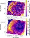 |
Fig. 5 Illustration of the profile variability with the peak position of the 6.2 μm PAH band (top) and the relative peak surface brightness of the 7.8 μm component with respect to the 7.6 μm component (bottom). Black and white contours represent the integrated 6.2 μm PAH surface brightness and the H2 0–0 S(7) integrated surface brightness, respectively (Fig. A.1). |
5.2 Disentangling the 11.2 μm feature
The 11.2 μm feature is known to have at least two components, namely the 11.207 μm one and the 11.25 μm one (Chown et al. 2024). Originally detected in the Orion Bar, the 11.207 μm component is attributed to PAH emission, while the broad 11.25 μm component is thought to be attributed to very small grains (VSGs) or PAH clusters (Chown et al. 2024; Pasquini et al. 2024; Khan et al. 2025). In the Orion Bar, the 11.25 μm VSG component is strongest in the H2 dissociation front and beyond. Following the method established by Khan et al. (2025), we isolated two components at 11.204 and 11.29 μm, referred to as the 11.207 and 11.25 μm components, respectively (Fig. 6; see Appendix E for details).
Spatial mapping (Fig. 7) reveals that the 11.207 μm component has a morphology akin to that of the 6.2 μm PAH feature, while the 11.25 μm component has a spatial distribution roughly resembling the H2 morphology, similar to the Orion Bar observations. This reinforces that the 11.25 μm component is indeed distinct from the PAH emission.
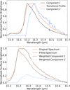 |
Fig. 6 Illustration of the 11.2 μm PAH band decomposition. Top: normalized profiles of the first component, with the narrowest profile representing class 𝒜, the broadest (transitional) profile representing class ℬ, and the second component used in the decomposition of the 11.2 μm feature. Bottom: typical decomposition of the 11.2 μm band by components 1 and 2. |
5.3 Correlation studies of the 6–9 μm features
Motivated by the significant profile variation in the 6.2 and 8.6 μm features, we performed a similar decomposition as was done for the 11.2 μm band to investigate whether the variation arises from the blending of two components. For the 6.2 μm feature, two components at 6.205 μm and 6.26 μm were successfully extracted and fit to reproduce all spectra (Fig. 8). The 6.205 μm component was the narrowest profile observed, whilst the 6.26 μm component was extracted via subtraction of the 6.205 μm component from the broadest profile observed. Fig. 9 shows two components successfully isolated from the 8.6 μm feature, at 8.56 and 8.65 μm. Here, the most redshifted 8.6 μm profile was assigned as the first component and subtracted from the 8.6 μm profile exhibiting the most blueshift to extract the second component. The weak 8.35 μm feature was extracted from the second component to isolate its emission. Details of the decompositions are found in Appendix E.
As the 7.6 and 7.8 μm components in the 7.7 μm feature trace class 𝒜 versus class ℬ PAH populations, respectively, a decomposition was performed to examine the spatial distribution of each component independently. To do so, we fit the 7–9 μm complex using four Gaussian components representing the 7.6, 7.8, 8.2, and 8.6 μm features, consistent with the approach of Peeters et al. (2017) and Stock & Peeters (2017), but adopting a broader 8.2 μm component. The data were well modeled with these Gaussian components and the integrated surface brightnesses of each component were measured (see Appendix E for details).
Analysis of component correlations provides further insight into the PAH interrelationships. Correlation plots between the 6.2, 7.7, and 8.6 μm components reveal that the blue components of the 6.2 and 7.7 μm bands (6.205 and G7.6 μm) are strongly correlated but neither are closely correlated with the blue or red component of the 8.6 μm band (Fig. 10). The three red components of the 6.2, 7.7, and 8.6 μm features (6.26, G7.8, and 8.65 μm) show tight correlations with each other, but none demonstrate correlations with the 6.205 and G7.6 μm components. The 8.56 μm component demonstrates an anticorrelation with the red components of the 6.2 and 7.7 μm components and is, therefore, separate from all other components. We refer the reader to Fig. F.1 for the correlation coefficients between all 6–9 μm components.
Examining component ratios (Fig. F.2) further highlights the uniqueness of the 11.25 μm component. The fractional contribution of the red component to the 6.2 (6.26/6.2), 7.7 (G7.8/7.7), and 8.6 (8.65/8.6) ratios strongly correlate with each other, yet none correlate with the fractional contribution of the VSG component to the 11.2 one (11.25/11.2), reinforcing the conclusion that the 11.25 μm emission arises from a carrier distinct from the carriers of the blue or red components of the 6.2,7.7, and 8.6 μm PAH bands.
We thus find four distinct PAH subpopulations: the red 6–9 μm components (6.26, 7.8, and 8.65 μm), associated with class ℬ populations; the blue 6.205 and 7.6 μm components, characteristic of class 𝒜 populations; the blue 8.56 μm component, the origin of which is explored in Section 6; and the 11.207 μm neutral PAH component. Additionally, the VSG/PAH cluster population is represented by the 11.25 μm component.
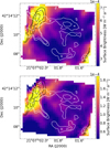 |
Fig. 7 Spatial maps of the integrated surface brightness of the 11.207 μm component (top) and of the 11.25 μm component (bottom). The contours are the same as in Fig. 5. |
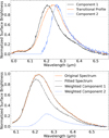 |
Fig. 8 Illustration of the decomposition of the 6.2 μm PAH band. Top: normalized profiles of the first component, with the narrowest profile representing class 𝒜, the broadest (transitional) profile representing class ℬ, and the derived second component used in the decomposition. Bottom: typical decomposition of the 6.2 μm band with components 1 and 2. |
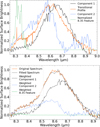 |
Fig. 9 Illustration of the decomposition of the 8.6 μm PAH band. Top: normalized profiles of the redshifted profile representing class ℬ (the first component), the blueshifted profile representing class 𝒜 (the transitional profile), the derived second component used in the decomposition, and the extracted 8.35 μm feature. Bottom: typical decomposition of the 8.6 μm band with components 1 and 2, and the 8.35 μm feature. |
6 Discussion
6.1 Spectral friends
The correlation observed between the 6.2 and 7.7 μm blue components (6.205 μm and 7.6 μm) and the red components (6.26 μm, 7.8 μm, and 8.65 μm) of the 6.2, 7.7, and 8.6 μm PAH bands (Sect. 5) suggests that these components originate from two distinct PAH subpopulations, with a separate third subpopulation represented by the blue 8.56 μm component of the 8.6 μm feature. Understanding the underlying origin of these spectral relationships is crucial.
Ricca et al. (2021) report that the 6.2 μm feature peaks at bluer wavelengths in elongated PAHs and at redder wavelengths in circular PAHs. Expanding on this result, Fig. 11 illustrates the harmonic density functional theory (DFT) calculations of the 6.2 and 7.7 μm peak positions for a set of PAH molecules, offering insight into potential carriers of these emission components. We use the NASA Ames PAH Infrared Spectroscopic Database1 version 4.0 (PAHdb; Bauschlicher et al. 2010; Boersma et al. 2014; Bauschlicher et al. 2018; Mattioda et al. 2020; Ricca et al. 2025) to relate the peak positions of the 6.2 and 7.7 μm bands to their corresponding molecular structures for a collection of seven PAH species. Only cationic PAHs were selected because the 6.2 and 7.7 μm bands are dominated by PAH cations (Hudgins & Allamandola 1999). We further constrained the subset of species by limiting ourselves to PAHs with long straight edges containing adjacent C-H solo bonds (also denoted as zigzag edges) because the 11.2 μm feature, attributed to the solo C-H out-of-plane bending mode, dominates the 10–15 μm C-H out-of-plane bending modes features, indicating that compact species dominate the PAH family (Hony et al. 2001; Ricca et al. 2018, 2021).
We find that the PAHdb calculations of the 6.2 and 7.7 μm peak positions of these species span the full wavelength range covered by the 6.2 and 7.7 μm components in NGC 7027 and that the precise positions of these features are unique for specific PAH molecules. If these findings are confirmed by quantum chemistry studies on a larger set of astrophysically relevant species, the peak positions of the components contributing to the 6.2 and 7.7 μm features could prove to be a useful diagnostic of PAH molecules in space. Based on this small sample, species with a similar structure to C62H20+ and C78H22+ appear to be good candidates for the 6.205 and 7.6 μm components, and molecules analogous to C66H20+ are potential carriers of the 6.26 and 7.8 μm components. We do not exclude, however, the possibility that each subpopulation originates not from a single PAH species, but is instead made up of a group of PAH species sharing similar spectral characteristics whose modes blend together into a single component. We do realize that the photochemical behavior of these putative species would have to be very similar as well to preserve the good correlations observed while the PAH population is being processed by the strong radiation field.
Previous analyses using PAHdb versions older than 4.0 have had issues explaining the class 𝒜 6.2 μm AIB as calculated peak positions of the carbon-carbon (CC) stretching mode in PAHs occurred at too red (i.e., ≃6.3 μm) of a wavelength. Subsequent DFT calculations on PANHs – PAHs with one or more N atoms substituted in their C skeleton – have revealed that the peak position is shifted toward the blue and such species can explain the peak position of class 𝒜 AIB profiles (Hudgins et al. 2005; Peeters et al. 2002). This has been taken to imply that PANHs are an important component in the interstellar PAH family (Boersma et al. 2013; Shannon & Boersma 2019; Rap et al. 2022). However, recent DFT studies established that earlier studies relied on calculations with basis sets that did not properly allow for polarization effects, and also that the use of more reliable basis sets results in CC modes spanning the full range (6.2–6.3 μm) of observed AIB peak positions (Ricca et al. 2021). Moreover, these new calculations demonstrate that PANHs have a strong out-of-plane mode at 11.0 μm. As this mode is very weak in AIB spectra, at most 10% of the 6.2 μm AIB could be ascribed to PANHs in the PAH family (Ricca et al. 2021). We note that Figure 11 is based on these improved DFT calculations.
We have limited our analysis to PAH cations. PAH anions also show CC modes in this wavelength range. However, with G0 = 6 × 10⁵ Habings, T = 2000 K, and n = 107 cm−3 (Tielens 2005), the PAH ionization parameter is γ = G0T1/2/ne ≃ 105 Habings K1/2 cm3 and the abundance of PAH anions in PDRs was calculated to be ≲1% (Sidhu et al. 2023). PAH anions are only abundant inside dense cores where they are protected from intense FUV radiation. This implies, however, that they are not exposed to the strong FUV field that can excite them. Hence, anions can be safely ignored in this analysis.
Previous studies link these PAH components to structural characteristics. For instance, Peeters et al. (2017) attribute the G7.6 μm component to compact, cationic, small PAHs and the G7.8 μm component to neutral, very large PAHs or PAH clusters. However, our results here are inconsistent with these findings. We instead see the G7.8/G7.6 μm ratio map (Fig. G.2) closely resembles the 6.2/11.207 ratio map (Fig. G.1), a known tracer of the ionic-to-neutral PAH ratio. This instead suggests that the conditions that favor the G7.8 μm component also favor charged PAHs, while the conditions that favor neutral PAHs also favor the G7.6 μm component. However, the C–C stretching modes are very weak in neutral PAHs (Hudgins & Allamandola 1999) and such species are not expected to contribute major features to the 6–9 μm range (Oomens et al. 2003; Bauschlicher et al. 2008). It is likely that these variations have no connection with PAH charge but instead with both PAH size and structure (Bauschlicher et al. 2008, 2009). It has been suggested that a red peak position of the 7.7 μm band is indicative of PAHs with ~96–130 C (Langhoff 1996; Bauschlicher et al. 2008; Joblin et al. 2008; Bauschlicher et al. 2009), albeit a few smaller-sized PAHs also show a red 7.7 μm band (see e.g., Fig 11). We do not see such a trend in the small subset of PAHs included in Fig. 11 due to its limited sample and size range.
Density functional theory studies imply that the intrinsic strength of the 8.6 μm in-plane C-H bending mode is a strong function of the PAH size and molecular structure (Bauschlicher et al. 2008, 2009; Ricca et al. 2012). Comparison of these quantum chemistry studies with observations implies that the 8.6 μm band is carried by a subset of compact PAHs with sizes in the range ~96–150 C atoms. Irregular or smaller compact PAHs do not show a very distinct 8.6 μm band while very large compact PAHs (>150 C atoms) show an 8.6 μm band that is much too strong compared to the C-C modes.
Given that the 6.205 and 7.6 μm components have no clear 8.6 μm counterpart, this serves as an indication that these blue components originate from medium-sized, asymmetric PAHs, consistent with Ricca et al. (2021). However, medium-sized asymmetric PAHs may be carriers of the weak 8.35 μm feature since these PAHs have intrinsically weak C-H in-plane bending modes. Unfortunately, as the 8.35 μm feature is a weak band perched on the side of the much stronger 8.6 μm feature, it is difficult to ascertain a strong link between the 8.35 μm feature and the 6.205 and 7.6 μm components. The subpopulation traced by the red components (6.26, 7.8, and 8.65 μm) is likely composed of compact PAHs within the ~96–150 C-atom size range, which is set by the 8.65 μm band. We note that the PAHs shown in Fig. 11 exhibit C–H in-plane bending emission shortward of 8.5 μm. The anticorrelation observed between the 8.56 μm component and the red components of the 6.2 and 7.7 μm features indicate that the same conditions that favor the 6.205 and 7.6 μm components, hamper the 8.56 μm one. The lack of correlation with any other component suggests that perhaps the 8.56 μm component stems from PAHs that are very large (>150 C atoms). In very large PAHs, the positive charge per carbon is very small and they behave more similarly to neutrals, which have insignificant 6.2 and 7.7 μm emission (Ricca et al. 2012). This is consistent with a scenario in which the smallest PAHs have been destroyed due to harsh photochemical processing in the nebula. Since the 3.3/11.2 PAH band ratio is a known diagnostic of PAH size (e.g., Allamandola et al. 1989; Pech et al. 2002; Ricca et al. 2012), future observations of NGC 7027 including the 3.3 μm feature would prove useful in linking the PAH size across the nebula to the variations found in this analysis of the 6.2, 7.7, and 8.6 μm features.
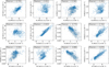 |
Fig. 10 Correlations between the 6.205, 6.26, G7.6, G7.8, 8.56, and 8.65 μm integrated component surface brightnesses normalized over the total 11.2 μm integrated surface brightness. Correlation coefficients are shown at the top and error bars are shown in light gray. |
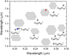 |
Fig. 11 6.2 and 7.7 μm peak positions of seven cationic PAH species (data taken from Ricca et al. 2021). Uncertainties for the theoretical band positions, calculated in Mackie et al. (2016, 2018) and Lemmens et al. (2019), are shown by the gray error bars (for details see Appendix H). The blue and red circles represent the observed peak positions of the blue and red components of the 6.2 and 7.7 μm bands in NGC 7027, respectively. |
6.2 PAH clusters and VSGs – Identity crisis of class ℬ11.2
The 6.2, 7.7, and 8.6 μm PAH bands exhibit class 𝒜, 𝒜ℬ, and ℬ profiles across the nebula. However, the variation in the 11.2 μm band is dominated by the contribution from the newly identified 11.25 μm component, which was extracted here for the first time in a PN. As has been demonstrated in Sect. 5, this component behaves distinctly from the PAH emission. Our results are consistent with the assignment of the 11.25 μm emission to PAH clusters and/or VSGs put forward by Chown et al. (2024), Pasquini et al. (2024), and Khan et al. (2025). Consequently, it is difficult to interpret the variation in the 11.2 μm feature as a shift in PAH spectral class since the 11.25 μm component over-shadows any subtle profile variations toward class ℬ. In fact, this component calls into question the existence of the 11.2 μm class ℬ profile defined in van Diedenhoven et al. (2004), as it is tarnished by the VSG contribution. The unique behavior of class ℬ11.2 was already noted in van Diedenhoven et al. (2004), where it was observed that class ℬ11.2 differs from class ℬ6–9. The recent discovery of the 11.25 μm component perhaps provides an explanation for the anomalous behavior of class ℬ11.2.
6.3 PAH evolution
The spatial distribution of PAH spectral classes observed within the nebula (Sect. 5) has the potential to provide valuable insights into the evolutionary processing mechanisms acting upon PAHs. Class ℬ profiles (which we attribute to large, compact PAHs with 96–130 C atoms) predominantly appear in the elliptical ring, while class 𝒜 profiles (which we attribute to medium-sized, asymmetric PAHs with 50–96 C atoms) appear in the region external to the ring.
We propose that the primary mechanism responsible for processing these PAHs is the star’s intense UV radiation (e.g., Cox et al. 2002; Moraga Baez et al. 2023). Consequently, these results suggest that the class ℬ PAHs are the material processed by UV radiation, while the class 𝒜 PAHs are unrefined and shielded from such energetic interactions. This is in line with laboratory studies and astronomical models that imply that smaller PAHs (class 𝒜) are more easily fragmented in a strong radiation field present near the PDR surface leaving the more robust larger PAHs (class ℬ) behind (Zhen et al. 2014b,a; Berné et al. 2015; Andrews et al. 2016; Panchagnula et al. 2024). Further astronomical observations focusing on the 3.3/11.2 μm AIB ratio, which is an established PAH size indicator (Croiset et al. 2016; Knight et al. 2021), can confirm the deduced differences in PAH size.
This is a slightly different scenario than originally suggested by Peeters et al. (2002) in which PAHs are injected by PNe into the ISM as class ℬ and the conversion to class 𝒜 occurs in the ISM, driven by the harsh radiation field. We emphasize, though, that the 5–15 μm spectra analyzed here are very consistent with predominantly aromatic materials (cf., Fig. 11). Near-infrared observations may provide insight into whether the photochemically driven loss of small PAHs in NGC 7027 is accompanied by a loss of aliphatic material, as seen in some post-AGB objects Goto et al. (2003, 2007).
We reconcile our results with earlier studies where class 𝒜 is observed in the ISM and class ℬ PAHs in PNe and protoplanetary disks as follows. In PNe, most of a star’s initial mass is expelled during the AGB phase. The majority of this ejected material is never ultimately processed by the star’s harsh UV radiation or shocks, preserving its original, pristine state as it migrates into the ISM. PAHs in the ISM, therefore, retain their original class 𝒜 spectral profiles, which is consistent with PAH observations in the ISM. Conversely, despite the cooler temperatures in protoplanetary disk environments, the class ℬ profiles observed could be linked to the strong radiation fields incident on these disks, effectively processing the PAH population.
Theoretical studies show that shocks can also process the circumstellar and interstellar PAH family (Micelotta et al. 2010). The circumstellar environment of NGC 7027 is heavily processed by the jet(s) emanating from the star(s) (Lau et al. 2016; Bublitz et al. 2023). However, the regions most heavily processed fall outside of the FOV of these observations. Future observational studies could be instrumental in testing these models and elucidating the effects of shocks on the PAH family in space.
7 Conclusions
We present, for the first time, high-resolution spectral data of the mid-IR PAH emission in NGC 7027 from JWST MIRI-MRS spectral cubes. Our findings are as follows:
We report the first observation of PAH spectral profile changes over different classes (here 𝒜, 𝒜ℬ, and ℬ) in each of the major features observed (6.2, 7.7, 8.6, and 11.2 μm) within a single extended target;
We decomposed the 6.2 μm feature into two new components at 6.05 and 6.26 μm, the 7.7 μm feature into two Gaussian components, G7.6 and G7.8 μm, and the 8.6 μm feature into two components at 8.56 and 8.65 μm. Correlation plots reveal that the 6.05 and G7.6 μm components are strongly correlated and the red components of the three features (6.26, G7.8, and 8.65 μm) exhibit a tight correlation, while no correlation is observed between the red and blue components of the features. The 8.56 μm component is not observed to have a strong relationship with any of the other components. We, therefore, hypothesize that these components represent three distinct PAH subpopulations, with the blue 6.2 and 7.7 μm components belonging to medium-sized asymmetric PAHs (e.g.,
![Mathematical equation: $\[\mathrm{C}_{62} \mathrm{H}_{20}^{+}\]$](/articles/aa/full_html/2026/03/aa57653-25/aa57653-25-eq1.png) ), the red 6.2, 7.7, and 8.6 μm components to large (96–150 C atoms), compact, symmetric PAHs, and the 8.56 μm component to very large PAHs (≥150 C atoms);
), the red 6.2, 7.7, and 8.6 μm components to large (96–150 C atoms), compact, symmetric PAHs, and the 8.56 μm component to very large PAHs (≥150 C atoms);A successful decomposition was performed of the 11.2 μm band into its two formerly reported components: 11.207 and 11.25 μm (Pasquini et al. 2024; Khan et al. 2025). We confirm that these components behave similarly in NGC 7027 as in previous studies of the Orion Bar, in which the 11.207 μm component represents the neutral PAH emission and the 11.25 μm component represents unique emission potentially from VSGs or PAH clusters, thus casting doubt on the existence of the class ℬ 11.2 μm profile as described by van Diedenhoven et al. (2004). The 11.2 μm band shows no clear counterpart to the red or blue components observed in the 6.2, 7.7, and 8.6 μm bands, nor is any link found between these components and the 11.25 μm component;
Class ℬ profiles were observed in the elliptical ring closer to the harsh UV radiation, whereas class 𝒜 profiles were detected further outside the ring. The profile variations across NGC 7027 therefore indicate that class 𝒜 PAH profiles, linked to the 6.205 and 7.6 components, presumably originate from less refined PAHs, and also that the class ℬ PAH emission, associated with the 6.26, 7.8, and 8.65 components, arises from more photo-processed PAH species. This implies that the majority of PAHs present in PNe enter the ISM as class 𝒜, shifting the perception of the evolution of PAH profile classes throughout the PAH life cycle.
Future spectroscopic work needs to be done to investigate the origin of the different PAH feature components and profile classes. Additional high-resolution spectral data from NGC 7027 and other PNe would help in disentangling the nature of PAHs in the early phases of their evolution.
Acknowledgements
We thank the referee for the helpful feedback. This work is based on observations made with the NASA/ESA/CSA James Webb Space Telescope. The data were obtained from the Mikulski Archive for Space Telescopes at the Space Telescope Science Institute, which is operated by the Association of Universities for Research in Astronomy, Inc., under NASA contract NAS 5-03127 for JWST. These observations are associated with program #1523 (DOI: 10.17909/5kp7-y840). Els Peeters acknowledges support from the Natural Sciences and Engineering Research Council of Canada. Alessandra Ricca acknowledges support from the Internal Scientist Funding Model (ISFM) Laboratory Astrophysics Directed Work Package at NASA Ames (22-A22ISFM-0009). This article is based upon work from COST Action CA21126 – Carbon molecular nanostructures in space (NanoSpace), supported by COST (European Cooperation in Science and Technology).
References
- Allamandola, L. J., Tielens, A. G. G. M., & Barker, J. R. 1989, ApJS, 71, 733 [Google Scholar]
- Andrews, H., Candian, A., & Tielens, A. G. G. M. 2016, A&A, 595, A23 [NASA ADS] [CrossRef] [EDP Sciences] [Google Scholar]
- Argyriou, I., Glasse, A., Law, D. R., et al. 2023, A&A, 675, A111 [NASA ADS] [CrossRef] [EDP Sciences] [Google Scholar]
- Balick, B., & Frank, A. 2002, ARA&A, 40, 439 [Google Scholar]
- Bauschlicher, Charles W., J., Peeters, E., & Allamandola, L. J. 2008, ApJ, 678, 316 [NASA ADS] [CrossRef] [Google Scholar]
- Bauschlicher, Charles W., J., Peeters, E., & Allamandola, L. J. 2009, ApJ, 697, 311 [NASA ADS] [CrossRef] [Google Scholar]
- Bauschlicher, Jr., C. W., Boersma, C., Ricca, A., et al. 2010, ApJS, 189, 341 [NASA ADS] [CrossRef] [Google Scholar]
- Bauschlicher, Jr., C. W., Ricca, A., Boersma, C., & Allamandola, L. J. 2018, ApJS, 234, 32 [NASA ADS] [CrossRef] [Google Scholar]
- Bernard Salas, J., Pottasch, S. R., Beintema, D. A., & Wesselius, P. R. 2001, A&A, 367, 949 [NASA ADS] [CrossRef] [EDP Sciences] [Google Scholar]
- Berné, O., Montillaud, J., & Joblin, C. 2015, A&A, 577, A133 [NASA ADS] [CrossRef] [EDP Sciences] [Google Scholar]
- Boersma, C., Hony, S., & Tielens, A. G. G. M. 2006, A&A, 447, 213 [NASA ADS] [CrossRef] [EDP Sciences] [Google Scholar]
- Boersma, C., Bouwman, J., Lahuis, F., et al. 2008, A&A, 484, 241 [NASA ADS] [CrossRef] [EDP Sciences] [Google Scholar]
- Boersma, C., Bregman, J. D., & Allamandola, L. J. 2013, ApJ, 769, 117 [NASA ADS] [CrossRef] [Google Scholar]
- Boersma, C., Bauschlicher, Jr., C. W., Ricca, A., et al. 2014, ApJS, 211, 8 [NASA ADS] [CrossRef] [Google Scholar]
- Bregman, J. D., Allamandola, L. J., Tielens, A. G. G. M., Geballe, T. R., & Witteborn, F. C. 1989, ApJ, 344, 791 [NASA ADS] [CrossRef] [Google Scholar]
- Bublitz, J., Kastner, J. H., Hily-Blant, P., et al. 2023, ApJ, 942, 14 [Google Scholar]
- Cherchneff, I., Barker, J. R., & Tielens, A. G. G. M. 1992, ApJ, 401, 269 [Google Scholar]
- Chown, R., Sidhu, A., Peeters, E., et al. 2024, A&A, 685, A75 [NASA ADS] [CrossRef] [EDP Sciences] [Google Scholar]
- Cohen, M., Allamandola, L., Tielens, A. G. G. M., et al. 1986, ApJ, 302, 737 [Google Scholar]
- Cohen, M., Tielens, A. G. G. M., Bregman, J., et al. 1989, ApJ, 341, 246 [NASA ADS] [CrossRef] [Google Scholar]
- Cox, P., Maillard, J. P., Huggins, P. J., et al. 1997, A&A, 321, 907 [Google Scholar]
- Cox, P., Huggins, P. J., Maillard, J.-P., et al. 2002, A&A, 384, 603 [NASA ADS] [CrossRef] [EDP Sciences] [Google Scholar]
- Croiset, B. A., Candian, A., Berné, O., & Tielens, A. G. G. M. 2016, A&A, 590, A26 [NASA ADS] [CrossRef] [EDP Sciences] [Google Scholar]
- De Marco, O. 2009, PASP, 121, 316 [NASA ADS] [CrossRef] [Google Scholar]
- Frenklach, M., & Feigelson, E. D. 1989, ApJ, 341, 372 [NASA ADS] [CrossRef] [Google Scholar]
- Galliano, F., Dwek, E., & Chanial, P. 2008a, ApJ, 672, 214 [NASA ADS] [CrossRef] [Google Scholar]
- Galliano, F., Madden, S. C., Tielens, A. G. G. M., Peeters, E., & Jones, A. P. 2008b, ApJ, 679, 310 [Google Scholar]
- Gardner, J. P., Mather, J. C., Clampin, M., et al. 2006, Space Sci. Rev., 123, 485 [Google Scholar]
- Goto, M., Gaessler, W., Hayano, Y., et al. 2003, ApJ, 589, 419 [NASA ADS] [CrossRef] [Google Scholar]
- Goto, M., Kwok, S., Takami, H., et al. 2007, ApJ, 662, 389 [NASA ADS] [CrossRef] [Google Scholar]
- Graham, J. R., Serabyn, E., Herbst, T. M., et al. 1993, AJ, 105, 250 [NASA ADS] [CrossRef] [Google Scholar]
- Hony, S., Van Kerckhoven, C., Peeters, E., et al. 2001, A&A, 370, 1030 [CrossRef] [EDP Sciences] [Google Scholar]
- Hudgins, D. M., & Allamandola, L. J. 1999, ApJ, 513, L69 [Google Scholar]
- Hudgins, D. M., Bauschlicher, Jr., C. W., & Allamandola, L. J. 2005, ApJ, 632, 316 [NASA ADS] [CrossRef] [Google Scholar]
- Joblin, C., Szczerba, R., Berné, O., & Szyszka, C. 2008, A&A, 490, 189 [NASA ADS] [CrossRef] [EDP Sciences] [Google Scholar]
- Kastner, J. H., Gatley, I., Merrill, K. M., Probst, R., & Weintraub, D. 1994, ApJ, 421, 600 [CrossRef] [Google Scholar]
- Kastner, J. H., Bublitz, J., Balick, B., et al. 2020, Galaxies, 8, 49 [Google Scholar]
- Khan, B., Abbott, B., Peeters, E., et al. 2025, A&A, 699, A133 [NASA ADS] [CrossRef] [EDP Sciences] [Google Scholar]
- Knight, C., Peeters, E., Stock, D. J., Vacca, W. D., & Tielens, A. G. G. M. 2021, ApJ, 918, 8 [NASA ADS] [CrossRef] [Google Scholar]
- Langhoff, S. R. 1996, J. Phys. Chem., 100, 2819 [Google Scholar]
- Latter, W. B., Dayal, A., Bieging, J. H., et al. 2000, ApJ, 539, 783 [NASA ADS] [CrossRef] [Google Scholar]
- Lau, R. M., Werner, M., Sahai, R., & Ressler, M. E. 2016, ApJ, 833, 115 [Google Scholar]
- Lemmens, A. K., Rap, D. B., Thunnissen, J. M. M., et al. 2019, A&A, 628, A130 [EDP Sciences] [Google Scholar]
- Mackie, C. J., Candian, A., Huang, X., et al. 2016, J. Chem. Phys., 145, 084313 [NASA ADS] [CrossRef] [Google Scholar]
- Mackie, C. J., Candian, A., Huang, X., et al. 2018, Phys. Chem. Chem. Phys. (Incorp. Faraday Trans.), 20, 1189 [Google Scholar]
- Masson, C. R. 1989, ApJ, 336, 294 [NASA ADS] [Google Scholar]
- Matsuura, M., Barlow, M. J., Zijlstra, A. A., et al. 2009, MNRAS, 396, 918 [NASA ADS] [CrossRef] [Google Scholar]
- Matsuura, M., Bernard-Salas, J., Lloyd Evans, T., et al. 2014, MNRAS, 439, 1472 [NASA ADS] [CrossRef] [Google Scholar]
- Mattioda, A. L., Hudgins, D. M., Boersma, C., et al. 2020, ApJS, 251, 22 [NASA ADS] [CrossRef] [Google Scholar]
- Micelotta, E. R., Jones, A. P., & Tielens, A. G. G. M. 2010, A&A, 510, A36 [NASA ADS] [CrossRef] [EDP Sciences] [Google Scholar]
- Moraga Baez, P., Kastner, J. H., Balick, B., Montez, R., & Bublitz, J. 2023, ApJ, 942, 15 [NASA ADS] [CrossRef] [Google Scholar]
- Nakashima, J.-i., Kwok, S., Zhang, Y., & Koning, N. 2010, AJ, 140, 490 [Google Scholar]
- Oomens, J., Tielens, A. G. G. M., Sartakov, B. G., von Helden, G., & Meijer, G. 2003, ApJ, 591, 968 [Google Scholar]
- Panchagnula, S., Kamer, J., Candian, A., et al. 2024, Phys. Chem. Chem. Phys. (Incorp. Faraday Trans.), 26, 18557 [Google Scholar]
- Pasquini, S., Peeters, E., Schefter, B., et al. 2024, A&A, 685, A77 [NASA ADS] [CrossRef] [EDP Sciences] [Google Scholar]
- Pech, C., Joblin, C., & Boissel, P. 2002, A&A, 388, 639 [NASA ADS] [CrossRef] [EDP Sciences] [Google Scholar]
- Peeters, E., Hony, S., Van Kerckhoven, C., et al. 2002, A&A, 390, 1089 [NASA ADS] [CrossRef] [EDP Sciences] [Google Scholar]
- Peeters, E., Bauschlicher, Charles W., J., Allamandola, L. J., et al. 2017, ApJ, 836, 198 [NASA ADS] [CrossRef] [Google Scholar]
- Rap, D. B., Schrauwen, J. G. M., Marimuthu, A. N., Redlich, B., & Brünken, S. 2022, Nat. Astron., 6, 1059 [Google Scholar]
- Ricca, A., Bauschlicher, Charles W., J., Boersma, C., Tielens, A. G. G. M., & Allamandola, L. J. 2012, ApJ, 754, 75 [NASA ADS] [CrossRef] [Google Scholar]
- Ricca, A., Bauschlicher, Jr., C. W., Roser, J. E., & Peeters, E. 2018, ApJ, 854, 115 [Google Scholar]
- Ricca, A., Boersma, C., & Peeters, E. 2021, ApJ, 923, 202 [NASA ADS] [CrossRef] [Google Scholar]
- Ricca, A., Boersma, C., Maragkoudakis, A., et al. 2025, ApJS, 282, 7 [Google Scholar]
- Shannon, M. J., & Boersma, C. 2019, ApJ, 871, 124 [NASA ADS] [CrossRef] [Google Scholar]
- Sidhu, A., Tielens, A. G. G. M., Peeters, E., & Cami, J. 2023, MNRAS, 522, 3227 [Google Scholar]
- Sloan, G. C., Lagadec, E., Zijlstra, A. A., et al. 2014, ApJ, 791, 28 [NASA ADS] [CrossRef] [Google Scholar]
- Smith, J. D. T., Draine, B. T., Dale, D. A., et al. 2007, ApJ, 656, 770 [Google Scholar]
- Stock, D. J., & Peeters, E. 2017, ApJ, 837, 129 [NASA ADS] [CrossRef] [Google Scholar]
- Tielens, A. G. G. M. 2008, ARA&A, 46, 289 [Google Scholar]
- Tielens, A. G. G. M. 2005, The Physics and Chemistry of the Interstellar Medium (Cambridge University Press) [Google Scholar]
- van Diedenhoven, B., Peeters, E., Van Kerckhoven, C., et al. 2004, ApJ, 611, 928 [NASA ADS] [CrossRef] [Google Scholar]
- Wells, M., Pel, J. W., Glasse, A., et al. 2015, PASP, 127, 646 [NASA ADS] [CrossRef] [Google Scholar]
- Wright, G. S., Wright, D., Goodson, G. B., et al. 2015, PASP, 127, 595 [NASA ADS] [CrossRef] [Google Scholar]
- Wright, G. S., Rieke, G. H., Glasse, A., et al. 2023, PASP, 135, 048003 [NASA ADS] [CrossRef] [Google Scholar]
- Zhang, Y., Liu, X. W., Luo, S. G., Péquignot, D., & Barlow, M. J. 2005, A&A, 442, 249 [NASA ADS] [CrossRef] [EDP Sciences] [Google Scholar]
- Zhen, J., Castellanos, P., Paardekooper, D. M., Linnartz, H., & Tielens, A. G. G. M. 2014a, ApJ, 797, L30 [Google Scholar]
- Zhen, J., Paardekooper, D. M., Candian, A., Linnartz, H., & Tielens, A. G. G. M. 2014b, Chem. Phys. Lett., 592, 211 [CrossRef] [Google Scholar]
- Zijlstra, A. A., van Hoof, P. A. M., & Perley, R. A. 2008, ApJ, 681, 1296 [NASA ADS] [CrossRef] [Google Scholar]
Appendix A NGC 7027 morphology
The morphological structures in the MIRI MRS CH1 FOV of NGC 7027 are demonstrated by the integrated surface brightness maps of the H I recombination line Pfund α (n=6-5), 6.2 μm PAH feature, and the H2 0-0 S(7) emission line, shown in Fig. A.1. The Pfund α emission traces the H II region which has the form of an elliptical shell. The 6.2 μm PAH emission sits just outside of the Pfund α emission and traces the atomic PDR, and morphologically resembles the ionized gas. Finally, the H2 emission outlines the surface of the molecular PDR.
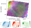 |
Fig. A.1 Three-color image of the 6.2 μm PAH feature (red), H2 0-0 S(7) emission line (green), and the Pfund α (n=6-5) emission line (blue) integrated surface brightness RGB maps in the NGC 7027 MIRI CH1 FOV (top). The individual integrated surface brightness images are shown in the bottom panels. |
Appendix B Extraction apertures
We utilize five extraction apertures in this study for the MIRI-MRS spectral cube and reference the ISO-SWS data. The information about the position and size each of these is given in Table B.1. The MIRI-MRS data have a position angle of 74.67°.
Information about the NGC 7027 extraction apertures utilized. Right ascension and declination (J2000) are given in [21:07:ss.ss] and [+42:14:ss.ss] respectively.
Appendix C Continuum determination
In order to isolate the PAH emission, the rising dust continuum emission and the emission from other contributors must be removed from the spectra. To trace out the continuum emission, we place anchor points at wavelengths solely probing the dust continuum emission and on either side of each PAH band.
We estimate the continuum emission for the MIRI-MRS spectral cube in two ways: one version has anchor points at 8.225 and 8.25 μm and another without anchor points around 8.2 μm (Fig. C.1). In addition, we fit both spectra with a plateau (PL) continuum, which is simply a linear fit between any two specified points and a spline curve (global spline, GS) elsewhere. The PL continuum is used to fit linearly underneath the main PAH features to avoid unusual effects from the spline curve which artificially augment or diminish the strength of the PAH emission. We thus use these PL continua for all plots and analysis.
Following the original classification of Peeters et al. (2002), we use the PL continuum with anchor points at ~8.2 μm for the profile classification of the 7.7 and 8.6 μm PAH bands. For all other analyses, the PL continuum without the anchor points at ~8.2 μm is used.
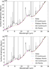 |
Fig. C.1 Illustration of the global spline (GS, orange) and plateau (PL, green) continuum without (top) and with (bottom) an anchor point near 8.2 μm for the MIRI-MRS integrated spectrum of NGC 7027. |
Appendix D Profile variability across NGC 7027
Table D.1 demonstrates a rich variety of PAH spectral characteristics of the ISO-SWS, MIRI-MRS, and spaxel apertures of NGC 7027 (Fig. 3; Table B.1). The outer NE corner is consistently characterized by class 𝒜 profiles, while the E and SW ring are consistently characterized by class ℬ profiles, with the exception of the class 𝒜ℬ 11.2 μm spectrum in SW ring. The spectra of ISO-SWS, MIRI-MRS, and the inner region, exhibit variation in spectral classes across the distinct PAH bands.
Overview of the PAH spectral classes in NGC 7027.
The 6.2 and 11.2 μm profile FWHMs across the nebula are measured. Fig. D.1 displays the changes in the profile widths across NGC 7027. Interestingly, the FWHM map of the 11.2 μm feature roughly follows the H2 contours.
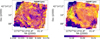 |
Fig. D.1 Profile width variability of the 6.2 (left) and 11.2 μm (right) features. The contours are the same as in Fig. 5. |
Appendix E Feature decompositions
Motivated by the decomposition performed on the 11.2 μm band by Khan et al. (2025), the 6.2 μm band is decomposed using the same method. We use the narrowest profile in the MIRI-MRS cube at 6.205 μm as the first component, and subtract this (scaled) component from the broadest profile in our mosaic to reveal component 2 which has a peak position of 6.26 μm (Fig. 8). Subsequently, we fit the 6.2 μm profile at each spaxel with a linear combination of these two components. This decomposition accurately models the 6.2 μm profiles observed in the mosaic (Fig. 8). The integrated surface brightnesses of each component are measured and used for analysis.
To reveal the contribution from each of the main PAH features within the 7-9 μm complex across the nebula, we fit the 7-9 μm complex using four Gaussian profiles to model the emission from the 7.6, 7.8, 8.2, and 8.6 μm features following the method used in Peeters et al. (2017) and Stock & Peeters (2017). We follow the methodology employed by Stock & Peeters (2017) to determine the peak position and FWHM of these Gaussians. The fitting routine tends toward a broad G8.2 component, rather than a narrow G8.2 (as done by Peeters et al. (2017) and Stock & Peeters (2017)). Subsequently, we fix the peak position (FWHM) to 7.636 (0.354), 7.889 (0.215), 8.042 (0.853), and 8.625 (0.305) μm, while we allow the amplitude to vary for each spectrum. We obtain very good fits to the spectra using a broad G8.2 μm component as shown in Fig. E.1, where the 8.2 μm component seems to represent both the 8.2 μm feature employed by these authors and the underlying 7–9 μm plateau upon which these four PAH bands sit.
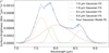 |
Fig. E.1 Four-Gaussian decomposition of the 7-9 μm complex employing a broad G8.2 profile for an example spectrum. Components are G7.6, G7.8, G8.2, and G8.6 μm. |
Given the variation in the 8.6 μm profiles, we perform a similar decomposition on this feature as done for the 6.2 μm band to reveal the potential underlying components. Here, we use the most redshifted profile in the MIRI-MRS cube at 8.65 μm as the first component, and subtract this (scaled) component from the profile exhibiting the largest blueshift to uncover component 2 with a peak position of 8.56 μm (Fig. 9). We extract the 8.35 μm feature which sits on top of the 8.56 μm component by subtracting a linear continuum underneath it. Subsequently, we fit the 8.6 μm profile at each spaxel with a linear combination of these two components and the 8.35 μm feature. The observed 8.6 μm profiles are well-modeled and the integrated surface brightnesses of each component are utilized for analysis.
Following the method in Khan et al. (2025), we consider the narrowest 11.2 profile in our mosaic as the primary component, which peaks at 11.204 μm, whereas in the Orion Bar the 11.207 μm component peaks at 11.20 μm. Second, we consider the broadest 11.2 profile in the spectral cube and subtract the scaled component 1 to obtain component 2, namely the 11.25 μm component, which peaks at 11.29 μm in NGC 7027 and in the Orion Bar (Khan et al. 2025). It is important to note that the primary component found here in NGC 7027 is broader than that of the Orion Bar, likely due to residual contamination from the secondary component, even in the narrowest profile. We attribute the slight differences in peak position to the decomposition method. Since the widest profile in NGC 7027 is broader than the widest profile in the Orion Bar, the 11.25 μm component here is also slightly broader than in the Orion Bar.
Using a linear combination of these two weighted components, we successfully decompose the 11.2 μm profile of each spaxel in the mosaic (see Fig. 6) and subsequently integrate the components to measure their integrated surface brightness spatially.
Appendix F Feature correlations
The heat-map highlighting the Pearson correlation coefficients between the 6-9 μm components is shown in Fig. F.1. All features are normalized over the 11.207 μm PAH component to remove any correlative behavior that is simply due to the contribution of the total PAH emission since we aim to uncover the underlying relationships between PAH components.
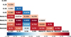 |
Fig. F.1 Heat-map demonstrating the strength of correlations between the 6-9 μm components when normalized to the 11.207 μm PAH component, where the intersection between two components displays their correlation coefficient. Redder boxes indicate a strong correlation, bluer boxes indicate a strong anticorrelation, and light boxes are present when there is little-to-no correlation. |
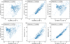 |
Fig. F.2 Correlation plots between the 6.26, 7.8, 8.65, and 11.25 μm components normalized over their feature totals. The Pearson correlation coefficient is shown in the top left corner of the plots. Error bars are shown in light gray. |
Figure F.2 shows no significant correlation between 11.25 and the red components of the 6.2, 7.7, and 8.6 μm features. On the other hand, the 6.26, G7.8, and 8.65 μm components demonstrate tight correlations with each other. Therefore, these plots serve as another indication that the 11.25 μm component exhibits unique behavior from the PAHs, while the 6.26, 7.8, and 8.65 μm components belong to the same PAH subpopulation.
Appendix G PAH band ratio maps
The ratio of the integrated surface brightness of PAH bands are calculated to reveal the relative strength of the features spatially. In particular, we calculate the 6.2/11.207 PAH band ratio since this ratio this is a known tracer of PAH charge. We use the 11.207 μm component since it contains only the PAH contribution to the 11.2 μm, without significant contamination from the 11.25 μm VSG/cluster component. The map reveals that, generally, the ionic PAHs dominate most in the ring. The ratio map of the G7.8/G7.6 PAH components is calculated and reveals a roughly co-spatial relationship with the 6.2/11.207 map.
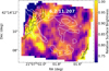 |
Fig. G.1 Spatial map of the 6.2 μm feature over the 11.207 μm component ratio. The contours are the same as in Fig. 5. |
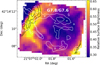 |
Fig. G.2 Spatial map of the G7.8 μm component over the G7.6 μm component ratio. The contours are the same as in Fig. 5. |
Appendix H Theoretical 6.2 and 7.7 μm band positions
It is worth noting that the calculations of the scaled harmonic peak positions of the 6.2 and 7.7 μm, such as in in Fig. 11, are accurate to 1.3% (Mackie et al. 2016; Lemmens et al. 2019).
For a set of small PAHs, the mid-infrared (5-18 μm) region has been studied in a cold molecular beam and modeled using anharmonic theory (Lemmens et al. 2019). Comparison between the FELIX free-electron laser experimental spectra and second-order vibrational perturbation theory calculations shows agreement in peak positions within ~0.5%, on average. Given that the FELIX bandwidth is ~1% of the photon energy, the theoretical values may in some cases be more accurate than the experimental determinations.
All Tables
Information about the NGC 7027 extraction apertures utilized. Right ascension and declination (J2000) are given in [21:07:ss.ss] and [+42:14:ss.ss] respectively.
All Figures
|
Fig. 1 MIRI-MRS integrated spectrum of NGC 7027 along with the PAH profile class 𝒜 (blue) and ℬ (red) for the 6.2, 7–9, and 11.2 μm features (exemplified by IRAS 23133+6050 and HD 44179 respectively; taken from Peeters et al. 2002; van Diedenhoven et al. 2004). |
| In the text | |
|
Fig. 2 Simplified schematic drawings of NGC 7027 as viewed from the side (top) and the front (bottom). The central star in shown in yellow. The H2 emission primarily lies on the surface of the biconical shell, and is particularly bright along the rims, while the ionized gas and PAHs reside within the elliptical ring. |
| In the text | |
|
Fig. 3 Top: HST/WFC3 NICMOS F212N image of NGC 7027 with JWST MIRI-MRS FOVs for channels 1 (red), 2, and 3 (white) overlaid. The black cross indicates the position of the central star. The yellow contours outline the H2 gas morphology in the continuum-subtracted HST/NICMOS images from Latter et al. (2000). The small orange, pink, blue, and green boxes are the spaxels used to illustrate the AIB variability referred to hereinafter as the E ring, outer NE corner, inner region, and the SW ring, respectively. Bottom: HST/WFC3 NICMOS F212N image of NGC 7027 with a schematic drawing overlaid. Credit: NASA/ESA, Latter et al. (2000). |
| In the text | |
|
Fig. 4 Illustration of the 6.2, 7–9, and 11.2 μm profile variation across the nebula. The single spaxel spectra from Fig. 3 detailed in Table B.1 are utilized here. |
| In the text | |
|
Fig. 5 Illustration of the profile variability with the peak position of the 6.2 μm PAH band (top) and the relative peak surface brightness of the 7.8 μm component with respect to the 7.6 μm component (bottom). Black and white contours represent the integrated 6.2 μm PAH surface brightness and the H2 0–0 S(7) integrated surface brightness, respectively (Fig. A.1). |
| In the text | |
|
Fig. 6 Illustration of the 11.2 μm PAH band decomposition. Top: normalized profiles of the first component, with the narrowest profile representing class 𝒜, the broadest (transitional) profile representing class ℬ, and the second component used in the decomposition of the 11.2 μm feature. Bottom: typical decomposition of the 11.2 μm band by components 1 and 2. |
| In the text | |
|
Fig. 7 Spatial maps of the integrated surface brightness of the 11.207 μm component (top) and of the 11.25 μm component (bottom). The contours are the same as in Fig. 5. |
| In the text | |
|
Fig. 8 Illustration of the decomposition of the 6.2 μm PAH band. Top: normalized profiles of the first component, with the narrowest profile representing class 𝒜, the broadest (transitional) profile representing class ℬ, and the derived second component used in the decomposition. Bottom: typical decomposition of the 6.2 μm band with components 1 and 2. |
| In the text | |
|
Fig. 9 Illustration of the decomposition of the 8.6 μm PAH band. Top: normalized profiles of the redshifted profile representing class ℬ (the first component), the blueshifted profile representing class 𝒜 (the transitional profile), the derived second component used in the decomposition, and the extracted 8.35 μm feature. Bottom: typical decomposition of the 8.6 μm band with components 1 and 2, and the 8.35 μm feature. |
| In the text | |
|
Fig. 10 Correlations between the 6.205, 6.26, G7.6, G7.8, 8.56, and 8.65 μm integrated component surface brightnesses normalized over the total 11.2 μm integrated surface brightness. Correlation coefficients are shown at the top and error bars are shown in light gray. |
| In the text | |
|
Fig. 11 6.2 and 7.7 μm peak positions of seven cationic PAH species (data taken from Ricca et al. 2021). Uncertainties for the theoretical band positions, calculated in Mackie et al. (2016, 2018) and Lemmens et al. (2019), are shown by the gray error bars (for details see Appendix H). The blue and red circles represent the observed peak positions of the blue and red components of the 6.2 and 7.7 μm bands in NGC 7027, respectively. |
| In the text | |
|
Fig. A.1 Three-color image of the 6.2 μm PAH feature (red), H2 0-0 S(7) emission line (green), and the Pfund α (n=6-5) emission line (blue) integrated surface brightness RGB maps in the NGC 7027 MIRI CH1 FOV (top). The individual integrated surface brightness images are shown in the bottom panels. |
| In the text | |
|
Fig. C.1 Illustration of the global spline (GS, orange) and plateau (PL, green) continuum without (top) and with (bottom) an anchor point near 8.2 μm for the MIRI-MRS integrated spectrum of NGC 7027. |
| In the text | |
|
Fig. D.1 Profile width variability of the 6.2 (left) and 11.2 μm (right) features. The contours are the same as in Fig. 5. |
| In the text | |
|
Fig. E.1 Four-Gaussian decomposition of the 7-9 μm complex employing a broad G8.2 profile for an example spectrum. Components are G7.6, G7.8, G8.2, and G8.6 μm. |
| In the text | |
|
Fig. F.1 Heat-map demonstrating the strength of correlations between the 6-9 μm components when normalized to the 11.207 μm PAH component, where the intersection between two components displays their correlation coefficient. Redder boxes indicate a strong correlation, bluer boxes indicate a strong anticorrelation, and light boxes are present when there is little-to-no correlation. |
| In the text | |
|
Fig. F.2 Correlation plots between the 6.26, 7.8, 8.65, and 11.25 μm components normalized over their feature totals. The Pearson correlation coefficient is shown in the top left corner of the plots. Error bars are shown in light gray. |
| In the text | |
|
Fig. G.1 Spatial map of the 6.2 μm feature over the 11.207 μm component ratio. The contours are the same as in Fig. 5. |
| In the text | |
|
Fig. G.2 Spatial map of the G7.8 μm component over the G7.6 μm component ratio. The contours are the same as in Fig. 5. |
| In the text | |
Current usage metrics show cumulative count of Article Views (full-text article views including HTML views, PDF and ePub downloads, according to the available data) and Abstracts Views on Vision4Press platform.
Data correspond to usage on the plateform after 2015. The current usage metrics is available 48-96 hours after online publication and is updated daily on week days.
Initial download of the metrics may take a while.