| Issue |
A&A
Volume 707, March 2026
|
|
|---|---|---|
| Article Number | A367 | |
| Number of page(s) | 12 | |
| Section | Planets, planetary systems, and small bodies | |
| DOI | https://doi.org/10.1051/0004-6361/202557725 | |
| Published online | 24 March 2026 | |
Weak S-type asteroids compared to C-type explain the observed size distribution of the main belt
1
Charles University, Faculty of Mathematics and Physics, Institute of Astronomy,
V Holešovičkách 2,
18000
Praha 8,
Czech Republic
2
Astronomical Institute of the Czech Academy of Sciences,
Fričova 298,
25165
Ondřejov,
Czech Republic
★ Corresponding author: This email address is being protected from spambots. You need JavaScript enabled to view it.
Received:
16
October
2025
Accepted:
4
February
2026
Abstract
The main belt, the region between the orbits of Mars and Jupiter, is home to more than 1 million asteroids. These asteroids form orbital groups, (i.e., asteroid families formed by collisions) and also spectral groups (taxonomies) with different chemical compositions, in particular carbonaceous (C-types) and silicate (S-types). In this paper, we extend the existing main-belt collisional model by finding the appropriate strength-versus-size dependence (also known as the scaling law) for these two groups. We used color indices and geometric albedos of 56 and 72 spectroscopically confirmed C- and S-types (control samples), along with statistical methods on 1 065 034 asteroids, to assign C-, S-, or other types. This allowed us to construct observed size-frequency distributions (SFDs) for several subpopulations constrained by either semimajor axis (inner, middle, outer) or taxonomy (C, S, other). Then we used a Monte Carlo collisional model to compute the long-term collisional evolution (4.5 billion years) and derive synthetic SFDs. Our best-fit scaling laws indicate that S-types must be weaker below approximately 0.2 km than C-types to explain the deficiency of asteroids in the inner part of the main belt near (and below) the observational limit. This may correspond to differences in chemical composition or material porosity. Future research will focus on the scaling laws of asteroids with rare or “extreme” taxonomies (e.g., V, M).
Key words: minor planets, asteroids: general
© The Authors 2026
 Open Access article, published by EDP Sciences, under the terms of the Creative Commons Attribution License (https://creativecommons.org/licenses/by/4.0), which permits unrestricted use, distribution, and reproduction in any medium, provided the original work is properly cited.
This article is published in open access under the Subscribe to Open model. This email address is being protected from spambots. You need JavaScript enabled to view it. to support open access publication.
1 Introduction
As the main belt (MB) represents a huge sample of more than 1 million asteroids (Tedesco & Desert 2002; Gladman et al. 2009), we need statistical descriptions of this sample. The appropriate description is the cumulative size distribution (hereafter SFD), i.e., the total number of asteroids N(≥D) greater than or equal to the size D. The characteristics of this distribution are affected by a series of processes, including collisions, fragmentation, ejection, perturbations by resonances, and the Yarkovsky effect, i.e., a drift of the semimajor axis due to thermal radiation forces (O’Brien & Greenberg 2005; Bottke et al. 2006; Vokrouhlický et al. 2015; Granvik et al. 2016).
One of the first efforts to explain the observed SFD was made by Anders (1965), who proposed that the initial (primordial) differential SFD was Gaussian. Later, this was disproved by Davis et al. (1979, 1985). The first analytical model was provided by Dohnanyi (1969), who showed that if the asteroid destruction rate is equal to their production rate, i.e., they are in collisional equilibrium (O’Brien & Greenberg 2003), then the cumulative SFD of these asteroids is described by a power law with slope −2.5. However, he did not use any realistic scaling laws. The first realistic scaling laws were used by Davis et al. (1979, 1985). They emphasized that precise collisional models should include other effects, for example, an orbital decay of asteroids over time. Later, Campo Bagatin et al. (1994) showed that scaling laws must be size-dependent to match the observations. An explicit form of the scaling law for the MB was found by O’Brien & Greenberg (2003, 2005).
In the following years, the collisional evolution of the MB was studied by several authors, focusing primarily on the characteristics of the evolved cumulative SFD. For example, Campo Bagatin et al. (1994) found a cutoff at small sizes; Bottke et al. (2005) showed that the cumulative SFD at large sizes is determined by early evolution of the MB from 4.5 to 3.9 Gyr ago; Cibulková et al. (2014) found that most asteroids appear monolithic rather than porous; and Bottke et al. (2015) noticed that the cumulative SFD is “wavy” for asteroids smaller than 10 km.
A substantial contribution is the work of Morbidelli et al. (2009), who published a Monte Carlo code Boulder for simulations of collisional evolution using a particle-in-a-box approach (Rubinstein & Kroese 2016). The code includes results from smoothed-particle hydrodynamic (SPH) simulations (Benz & Asphaug 1999; Cossins 2010; Jutzi 2015), which approximate a projectile and a target by thousands to millions of particles, tracking the relevant physical quantities. Morbidelli et al. (2009) themselves studied the primordial SFD of planetesimals.
Collisions are necessary to explain a number of other observations. They can, for example, explain the formation of comets (Bottke et al. 2022), the origin of dust in the Solar System (Landgraf et al. 2002; Nesvorný et al. 2006), the presence of nonindigenous material on Vesta, Bennu, and Almahata Sitta (Bottke et al. 2020a), asteroid shapes (Marchis et al. 2021; Brož et al. 2022), and cratering on asteroids (Bottke et al. 2020b).
Last but not the least, collisions are crucial for the formation of asteroid families (Michel et al. 2001; Zappalà et al. 1990; Nesvorný et al. 2002; Vokrouhlický et al. 2006). Collisional models can also help identify families (Nesvorný et al. 2015), estimate their age (Nesvorný et al. 2006; Vokrouhlický et al. 2010), describe their evolution (Vernazza et al. 2018), and study material strength (Marschall et al. 2022).
In this paper, we continue these studies by extending the collisional model of the MB. In particular, we split the MB into C-and S-types, since these two spectral (taxonomic) groups are the most common (Gradie & Tedesco 1982; Tholen 1984). Our goal is to find explicit forms of their scaling laws. To do so, we need to set up proper initial conditions and scaling laws for both populations and simulate their long-term collisional evolution. The resulting synthetic cumulative SFDs are then compared to the corresponding observed SFDs.
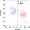 |
Fig. 1 Scatter plot of the C- (blue) and S-type (red) control samples in the i - z vs. a* plane, along with their uncertainties σi-z and σa*. |
2 Identifying C- and S-types in catalogs
The characteristics of reflectance spectrum determine the taxonomy of an asteroid (Bus & Binzel 2002a; DeMeo et al. 2009). These characteristics can also be described by magnitudes measured in several passbands - for example, g, r, i, z as measured by the Sloan Digital Sky Survey (SDSS) (Blanton et al. 2017). Their mutual subtraction yields distance-independent color indices. The indices are further calibrated by subtracting the values corresponding to the solar analog (Ivezić et al. 2001). For us, the most relevant color indices are i - z and the first principal component (denoted a*), obtained via principal component analysis by Ivezić et al. (2001). The two most populous taxonomies, i.e., C- and S-types are distinctive in a*, i – z, and the geometrical albedo pV (Zellner 1979; Ivezić et al. 2001; Delbo 2004; Parker et al. 2008).
2.1 Control sample of C- and S-types
To define our control samples, we first retrieved 328 C-type and 491 S-type asteroids identified by Bus & Binzel (2002a,b) during a spectroscopic survey of the MB. Their a* and i – z values were obtained from the SDSS catalog (Blanton et al. 2017), and their albedos from the AKARI (Yamauchi et al. 2011) catalog or, if unavailable, the Wide-field Infrared Survey Explorer (WISE; Masiero et al. 2011) catalog.
The C- or S-type was appended to the respective control sample if it satisfied three criteria: all values of a*, i – z, and pV known; uncertainties σa*, σi-z, and σpV below 0.1; and semimajor axis (proper or osculating) in the range 2.05-3.8 au. Applying these constraints yielded 56 C-types and 72 S-types. The scatter plots of both control samples are shown in Figs. 1 and 2. Within the uncertainties, C-types have negative a*, and S-types have positive a*, in agreement with Parker et al. (2008). A few C-types, however, have pV > 0.1, which is more typical of X-types, especially M-types in Tholen’s taxonomy (Tholen 1984) with a median of 0.17 (Bus & Binzel 2002a). These cases may represent other types but were retained in the C-type control sample.
2.2 Algorithm for an assignment of C-types, S-types, and other types
We implemented a Monte Carlo algorithm to assign C-, S-, or neither C- nor S-type (hereinafter, other type) to every asteroid with unknown taxonomy, using our control samples. The details are described in Vávra (2024) and in Appendix D.
As a result, from 1 065 034 asteroids, we obtained 601 213 C-and 453 998 S-types. Their spatial distribution is shown in Fig. 3. S-types prevail in the inner part of the MB, but as the semimajor axis increases, they are gradually overtaken by C-types, in agreement with Ivezić et al. (2001), Mothé-Diniz et al. (2003), and Marsset et al. (2022). Specifically, S-types comprise 58% of the inner MB, while C-types comprise 52% and 75% of the middle and outer parts, respectively. Other types represent only 1% of all asteroids.
2.3 Observational incompleteness
We estimated the observational limit size from the differential distribution of absolute magnitudes H, as in Hendler & Malhotra (2020). The method is based on the maximum absolute magnitude Hmax of the differential distribution. Below this value (H < Hmax), a population is considered complete, i.e., unbiased. The differential magnitude distributions N(H) for C-, S-, and other types are shown in Fig. F.1. We set the binning of the differential distributions to dH = 0.1 mag. The most populated bins for C-, S-, and other types are located at 17.00, 17.63, and 17.37 mag, respectively.
We then computed corresponding sizes for all absolute magnitudes within the most populated bin. For C-types, for example, H ranged from 16.95 to 17.05 mag. To compute D, we used the standard formula (Bowell et al. 1989)
![Mathematical equation: D = 10^{0.5[6.259-\log_{10}pV-0.4H]}\,.](/articles/aa/full_html/2026/03/aa57725-25/aa57725-25-eq1.png) (1)
(1)
From these sizes, we constructed a “tiny” differential SFD N(D), with binning dD = 0.1 km, as shown in Fig. F.2. If the differential SFD was unimodal, we used the 16% and 84% percentiles (to suppress outliers). If it was bimodal - because it contained a “mix” of other taxonomies - we used the 8% and 92% percentiles. We assumed that the observational limit size, or rather a transition from completeness to incompleteness, is between these percentiles. Hence, the observational limits are as follows: For C-types, 1.7 and 2.6 km; S-types, 0.7 and 1.0 km; other types, 0.7 and 2.1 km; the whole MB, 1.0 and 2.5 km; the inner part, 0.5 and 1.3 km; the middle part, 0.7 and 2.0 km; and the outer part, 1.2 and 2.8 km. In the following, the upper bound of each size range is adopted as the respective observational limit.
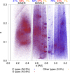 |
Fig. 3 Scatter plot of eccentricity vs. semimajor axis (both proper or osculating) for all resulted 601 213 C-, 453 998 S-, and 9823 other types across different parts of the MB (inner, middle, and outer) separated by vertical black lines. Above the plot are the relative numbers of each taxonomy (blue for C-, red for S-, and orange for other types) within the specific parts of the MB. |
2.4 Distributions of sizes
Finally, we computed sizes for all 1 065 034 asteroids and constructed the observed cumulative SFDs for the whole MB, its parts (inner, middle, outer), and C-type, S-type, and other taxonomies. The borders of the parts are based on the positions of the Kirkwood gaps (Kirkwood 1860). In particular, the inner borders lie at 2.05 and 2.502 au, the middle at 2.502 and 2.825 au, and the outer at 2.825 and 3.25 au. Substantial differences appear among individual SFDs, namely the power-law slopes in different ranges, the cumulative number of asteroids N(≥D), the presence of “knees” (where the SFDs change slopes), and the observational limits. The SFDs are shown in Figs. 4 and 5.
The differences are intrinsic properties of the populations. For the inner, middle, and outer parts, this is obvious, as they were split according to semimajor axis. For the C-types, S-types, and other types, the differences among SFDs are not “artifacts” of our method (Sect. 2.2), because the surveys’ completeness (0.5-2.5 km) is already sufficient to observe them. Using a different method (e.g., based only on pV) would lead to similar results.
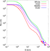 |
Fig. 4 Observed SFD of the entire MB (green) and its individual parts: inner (red), middle (magenta), and outer (blue). We highlight the three largest asteroids in each region: inner - (19) Fortuna, (7) Iris, and (4) Vesta (red points); middle - (15) Eunomia, (2) Pallas, and (1) Ceres (magenta points); and outer - (704) Interamnia, (52) Europa, and (10) Hygiea (blue points). The “star-shaped” points on each SFD mark the limit size ranges obtained in Sect. 2.3, below which the data are observationally incomplete for the entire MB (green), inner (red), middle (magenta), and outer (blue) parts. The observed SFDs differ significantly, even above 100 km, where collisional evolution is negligible, implying different initial conditions. |
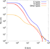 |
Fig. 5 Same as Fig. 4, but for C-types (blue), S-types (red), and other types (orange). We include: the five largest C-types - (1) Ceres, (10) Hygiea, (52) Europa, (511) Davida, and (31) Euphrosyne (blue points); S-types - (15) Eunomia, (7) Iris, (3) Juno, (532) Herculina, and (29) Amphitrite (red points); and other types (4) Vesta, (2) Pallas, (704) Interamnia, (65) Cybele, and (87) Sylvia (orange points). |
3 Collisional models with fixed rheology
Collisional models of the MB vary in complexity. For simplicity, single or “mean” rheology is assumed for all populations. Here, we thoroughly test models with single rheology but different numbers of populations (one to three).
For all main-belt populations, we prescribed the decay timescales τmb(D) for various sizes, as in Brož et al. (2024), in agreement with the observed near-Earth object (NEO) population (see their Fig. B.3). The decay timescales τmb directly determine the influx of NEOs, while the decay timescales τneo of NEOs determine their outflux. If the influx or outflux is incorrect, the synthetic versus observed SFDs of NEOs do not match. For simplicity, we assumed that τmb is the same for all populations. However, each population were required to have different collisional probabilities and impact velocities.
For each model and each population involved, we set the initial SFDs to follow a pattern similar to the observed SFDs but with higher cumulative numbers N(≥D), i.e., their initial SFD lies above the observed one. This excess was used because long-term collisional evolution inevitably leads to a temporal decrease in N(≥D). The smaller the size D, the higher excess. The observed SFD of each population is different (cf. Figs. 4 and 5); therefore, the initial SFD for each population must also be different. In this context, the term “initial” means after early bombardment by leftover planetesimals (Nesvorný et al. 2023), after giant-planet instabilities (Deienno et al. 2024, 2025), and after implantation of C-type bodies (Anderson et al. 2025). We do not refer to post-accretion SFDs, which could be very similar in different parts of the belt.
Using the Monte Carlo collisional code Boulder (Morbidelli et al. 2009; Vernazza et al. 2018), SFDs were collisionally evolved for up to 4.5 billion years. Each was evolved 100 times (100 simulations) with different random seeds due to the intrinsic stochasticity of large disruptions. The set of synthetic SFDs was then compared to the observed SFD discussed in Sect. 2.4. We primarily focused on how many synthetic SFDs lay below or above the observed one. If the majority (e.g., more than 60) lay significantly below, we considered the simulation problematic. This occurred especially at sizes D < 4 km, i.e., close to the observational limit. If more asteroids had been detected below this size, the observed SFD would have increased and differed even more from the synthetic SFDs. We thus manually adjusted the initial SFDs and ran the simulations again.
3.1 Scaling law
To describe the tendency of a target to be disrupted, we must directly measure or simulate collisions between targets and projectiles under different scenarios - namely, with different impact velocities, impact angles, and different sizes. In case of direct measurements, we are limited to very small target sizes; for example, Gault et al. (1963) used centimeter-sized rocky targets, while Fujiwara et al. (1977), Davis & Ryan (1990), and Nakamura et al. (1992) used up to 10 cm-sized, and Capaccioni et al. (1986) 30 cm-sized ones. On the other hand, as far as simulations are concerned, we can use results from hundreds of SPH simulations performed on much larger targets than those in laboratory experiments (e.g., Benz & Asphaug 1994, 1995, 1999; Love & Ahrens 1996; Durda et al. 2007; Jutzi et al. 2008, 2010; Jutzi 2015; Schwartz et al. 2016; Ševeček et al. 2017, 2019; Vernazza et al. 2018; Rozehnal et al. 2022). As a result of such calibrated simulations, we can obtain the so-called scaling law for the target.
We adopted the scaling law from Benz & Asphaug (1999) in the form
![Mathematical equation: Q^*(D)\equiv {1\over q}\left[Q_0\left(\frac{D}{D_0}\right)^a+B\rho \left(\frac{D}{D_0}\right)^b\right],](/articles/aa/full_html/2026/03/aa57725-25/aa57725-25-eq2.png) (2)
(2)
where D [cm] is the target size (diameter); D0 [cm] is the normalization size; Q* [erg g−1] is the energy of the impact per unit mass of the target required to disperse 50% of the target (Durda et al. 1998; O’Brien & Greenberg 2003); a, b, B [erg g−2], q, and Q0 [erg g−1] are free parameters; and ρ [g cm−3] is the density of the target.
As shown by Benz & Asphaug (1999), the free parameters a, b, B, and Q0 depend on the impact velocity as well as on the material. They performed several SPH simulations to derive the free parameters for basalt and ice. We used their scaling law for basalt, which was slightly adjusted (see the discussion in Vernazza et al. 2018). The respective parameters were q = 1, D0 = 2cm, ρ = 3 g cm−3, Q0 = 9 ∙ 107ergg−1, B = 0.5 ergg−2 cm3, a = −0.53, and b = 1.36.
3.2 Collisional probabilities and impact velocities
We determined the collisional probabilities and impact velocities between individual populations using the Öpik formalism (Öpik 1951; Greenberg 1982; Bottke & Greenberg 1993). The quantities were computed for individual pairs of asteroid orbits, based on their osculating semimajor axis, eccentricity, and inclination. To reduce computational time, we selected 1000 non-repeating random orbits from each population. The resulting mean values are summarized in Table E.1.
3.3 Initial differential SFDs
We generated initial differential SFDs as a set of points:  . These points follow a pattern prescribed by a piece-wise power-law function, with a negative slope(s) γ for a specific size range(s), dN(D) = CDγ, where C is a constant. The number of slopes is three, four, or five; the slopes, along with their respective size ranges, are considered free parameters. The bins were logarithmically spaced, and neighboring bin centers had a fixed ratio of 1.15. The normalization number nnorm for the normalization size dnorm is given for the corresponding cumulative distribution, nnorm = N(≥dnorm). The respective relation is
  , and the power-law slope thus differs by one: N(≥D) = C, Dκ, where C′ is a constant and κ = γ + 1. Additionally, the initial SFDs did not include the largest asteroids; therefore, we added them manually to respective populations.
3.4 One main belt population
As a verification, we simulated the collisional evolution of the entire MB population. We tested two different types of the initial SFDs - “no tail” and “with tail.” Both followed a pattern similar to the observed SFD, down to D = 4 km. The three largest asteroids (1) Ceres, (2) Pallas, and (4) Vesta were added manually. Both types of initial SFDs, along with their respective synthetic SFDs, are shown in Figs. F.3, F.4. We see that both initial conditions resulted in synthetic SFDs matching the observed SFD, in agreement with Bottke et al. (2005, 2020b). Therefore, it does not matter which type is chosen; for the initial SFDs in subsequent models, we used only the first type.
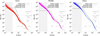 |
Fig. 6 Initial SFD (black), 100 evolved SFDs of the inner (red), middle (pink), and outer (blue) parts, and their respective observed SFD (green). The vertical dashed gray lines represent size ranges where the initial SFD was approximated by a different power law, i.e., a different slope. For the inner part, for example, the slopes are −3.55 above 100 km, −2.30 between 100 and 60 km, −1.65 between 60 and 15 km, and −4.00 between 15 and 3 km. The last slope below 3 km was set to zero, i.e., a constant cumulative SFD (“no tail”). Individual slopes are shown in gray within the panels at the respective size ranges. Density ρ, normalization size dnorm, and the normalization number nnorm for each part are shown on the right side of the respective panel. The gray areas correspond to the size ranges below the observational limits. The problem in the inner part is that most evolved SFDs lie below the observed SFD below D ~ 3 km. |
3.5 Inner, middle, and outer parts
When we split the MB into three parts - inner, middle, and outer - the situation was different. It was very difficult to set the correct initial SFDs for each part: changing one parameter in one initial SFD affected the evolved SFDs of all three parts because the respective collisional probabilities are nonzero (Table E.1). For the inner belt, in particular, we tested a number of different slopes: κ4 ∈ {−4.0, −4.5, −5.0}, κ3 ∈ {−1.8, −1.7, −1.65}, and κ2 ∈ {−2.2, −2.3, −2.4}. Our best initial SFDs, along with each simulation, are shown in Fig. 6.
Overall, the sum of all three SFDs matches the observed SFD (Fig. F.5). However, there are imperfections in the individuals parts: i) every evolved SFD of the outer part lies above the observed one between 21 and 47 km; ii) the majority of the evolved SFDs of the middle part lies above the observed one between 5 and 10 km; and iii) the majority of the evolved SFDs of the inner part lies below the observed one below D ≈ 3 km. The last imperfection is the most crucial because more than 90% of evolved SFDs of the inner part lie below the observed SFD. This imperfection persists to sizes below the observational limit at 1.3 km, which is even worse, because the debiased observed SFD would lie even further above. We found no “triad” of initial SFDs that resolves this deficiency.
3.6 C-types, S-types, and other types
When we split the MB into three taxonomies - C-types, S-types, and other types - the situation was the same. C-type density was set to 1.7 g/cm3, and S-type density to 3.0 g/cm3 (Vernazza et al. 2021). Our best initial SFDs, along with individual simulations, are shown in Fig. 7.
Both C- and S-types exhibit the same problem as in the inner part. In particular, the most evolved C- and S-types lie below the respective observed ones below 7 and 4 km, respectively. The most crucial problem, though, is the fact that 94 and 69 evolved SFDs of C- and S-types, respectively, lie below their observed SFDs at the observational limits (2.6 km for C-types; 1 km for S-types). We found no initial SFDs that resolved these deficiencies.
Problem with other types. Moreover, the observed SFD of other types is clearly too shallow (Fig. 7, right). The “tail” should always be Dohnanyi-like, with a slope of approximately −2.5. Indeed, evolved SFDs of other types are always steep below D ≈ 10 km. The observed other types must therefore be incorrect, i.e., some observed (assigned) C- and S-types must actually be other types. Conversely, including all other types in C- or S-types could potentially solve these deficiencies.
We thus tried to reassign all observed other types to C-types, creating a “mix” of C- and other types. Of course, the initial SFDs of this “mix”, along with S-types, had to be modified due to their mutual collisions. This partially solved the problem, but only for C-types. Out of 100 simulations, only 40% were below the observed SFD (at or below 2.6 km), which is acceptable. However, S-type deficiency remained: out of 100 simulations, 70% were below the observed SFD (at or below 1.0 km). Consequently, this is only a partial solution.
We also tried to reassign other types to S-types, but this model was inconsistent. This “mix” exhibited an excess at multikilometer sizes, which contradicts our results for the inner belt (Sect. 3.5). Moreover, SMASSII spectra of other types were mostly B-types (with affinity to C-types) and X-types, which appear distributed across the belt - unlike S-types, which should prevail in the inner belt.
Another solution would be to modify our algorithm for assigning C- and S-types, i.e., to tighten the condition for classifying asteroids with unknown taxonomy as C- or S-type, making them less numerous. However, the “ultimate” solution is to modify the rheology (scaling law) for S-types because SFD characteristics depend sensitively on the slope and, in particular, the position of the scaling-law minimum (Marschall et al. 2022). On the other hand, the rheology of C-types should remain similar to the entire MB, because C-types comprise ~80% of the multi-kilometer population (Fig. 5).
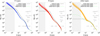 |
Fig. 7 Same as Fig. 6 for the C-types, S-types, and other types. The problem with both C- and S-types is that most evolved SFDs lie below the observed SFD below D ~ 7 and 4 km, respectively. Conversely, evolved SFDs of other types always lie above the observed SFD (see text for discussion). |
4 Collisional models with variable rheology
In more complex models, each population can have distinct rheology. In the case of C- and S-types, differences arise due to their chemical and mineralogical composition: C-types are carbonaceous, and S-types are silicate. Vernazza et al. (2021) showed that C- and S-types differ further in bulk density (1.7 vs. 3.0 g cm−3 for D ≳ 100 km); porosity (20 vs. 8%); and shape (higher sphericity index for C-types). Furthermore, the ratio between the critical periods (the spin barrier) of C- and S-types depends on their cohesive strengths; Carbognani (2017) estimated that the cohesive strength of C-types is higher than that of S-types by 40%. All these properties were inferred from adaptive-optics imaging surveys (Vernazza et al. 2021), spectroscopic surveys (Bus & Binzel 2002b; Binzel et al. 2019), and light curve inversion (Warner et al. 2009; Ďurech et al. 2010, 2019).
Regarding material properties, laboratory measurements were conducted on meteorites, with compositions similar to C-and S-types - namely, carbonaceous and ordinary chondrites. They primarily contain different amounts of carbon or silicates (Hutchison 2007) and also differ in bulk and grain density and hence porosity (Consolmagno et al. 2008; Macke et al. 2011). All these examples strongly suggest that C- and S-types have distinct rheology.
To solve the deficiencies of the inner part and S-types (Sects. 3.5, 3.6), we tried modifying the scaling law. We proposed three ideas. Specifically, we either made asteroids
below the scaling-law minimum stronger, so that they more easily disrupted those at the minimum, making them less numerous and thus unable to disrupt even bigger ones; or
made asteroids at and below the minimum weaker, so that they did not disrupt those above the minimum; or
made asteroids below the minimum weaker and those above stronger to preserve them.
In the context of Eq. (2), these ideas correspond to properly lowering a, increasing D0, and lowering q (i.e., idea 1); lowering Q0 (idea 2a) or a (idea 2b); or lowering D0 (idea 3); which simultaneously shifts the scaling-law minimum, as shown in Fig. 8.
We tested these ideas on the entire MB population to determine which ones substantially increase the SFDs at sizes near (and below) the observational limit. We rejected idea 1, because it did not substantially increase the SFDs. We also rejected idea 2a because it resulted in roughly the same increase as idea 2b. Hereinafter, we refer to idea 2b as idea 2.
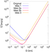 |
Fig. 8 Original scaling law (gray) and its modifications (labeled here as “ideas”), plotted in blue, pink, red, and orange. |
4.1 Fitting scaling laws - inner, middle, and outer
For the inner part of the MB, we tested 12 different scaling laws. For idea 2, we used values a ∈ {-0.60, −0.65,..., −0.86}, while for the idea 3, we used D ∈ {1.9,1.8,..., 1.4} cm (cf. a = −0.53 and D0 = 2cm in Sect. 3.1). The corresponding set of scaling laws is shown in Fig. 9.
Compared to the SFDs for the original scaling law (left panel in Fig. 6), the SFD of the inner belt increased most for a = −0.86, without considerable change in the SFDs of the other two parts. However, the initial conditions were modified accordingly; we tried 25 different initial SFDs. The best final SFDs, in comparison to those observed, are shown in Fig. 10. At the observational limit (D = 1 km), 52% of the final SFDs lies below the observed SFD, which is acceptable. Unfortunately, a minor excess appears between approximately 3 and 7 km. Some initial conditions resolved this excess; however, they led to a substantial decrease below the observational limit, which would eventually bring us back to the original problem. Still, we conclude that idea 2 is acceptable. For the idea 3, we obtained comparable results if D0 = 1.4 cm, but at the expense of considerable excess of multi-kilometer bodies; we thus consider idea 3 less acceptable.
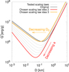 |
Fig. 9 Twelve scaling laws (gray) tested for the inner belt, compared to the original (black) from Sect. 3.5. Those, which substantially increased the evolved SFDs below the observational limit, are shown in red and orange. The directions of scaling law minimum changes for decreasing a and D0 are shown by red and orange arrows, respectively. |
4.2 Fitting scaling laws for C- and S-types
Since the inner part is mostly composed of S-types, we used the same modified scaling law for them as for the inner part (idea 2) to see if it solved the deficiency at small sizes. For C-types, we kept the original scaling law, namely, the one used in Sect. 3. To select the best pair of initial SFDs for C- and S-types, we defined the goodness of the fit in terms of the “pseudo” χ2 (Cibulková et al. 2014). It is called “pseudo” because we used only formal uncertainties and did not perform a statistical χ2 test to determine a statistical significance of the fit. The definition of χ2 is discussed in Appendix C.
We tested six different initial SFDs for C-types. For S-types, we tried the original plus two modifications because we expected an increase in C-types to create more projectiles that could potentially disrupt some S-types. The total number of initial SFD pairs was 18 (Fig. F.6). For each pair, we computed the collisional evolution and corresponding χ2. The χ2 was evaluated between the observational limit and 120 km and 60 km, for C- and S-types, respectively. We chose these limits because the observed SFDs are “jaggy” above these sizes, which would bias χ2.
The best-fit collisional model, with the lowest χ2 = 50.0, is shown in Fig. 11. It is a significant improvement with respect to the original initial SFDs (χ2 = 197.9). This corresponds to better than 10% agreement with the observed SFDs. The statistical distribution of 100 synthetic SFDs is even: approximately 50 lie above, and 50 lie below the observed SFD for sizes above the observational limit. More importantly, almost no synthetic SFDs “undershoot” the observed SFD for sizes below the observational limit. In this sense, our collisional model is self-consistent and explains the observed SFDs of both C- and S-types.
The explicit forms of our best-fit scaling laws for C- and S-types are as follows:
 (3)
(3)
 (4)
(4)
where QC,S* is in ergs per gram and R = D/2 is in centimeters. These formulæ demonstrate that S-types are significantly weaker than C-types at sizes D ≲ 0.2 km below the current observational limits. This weakness, however, is seen due to collisional cascade at sizes D ≳ 1 km above the limits.
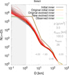 |
Fig. 10 Same as Fig. 6, for the inner part and a modified scaling law (“idea 2”). For comparison, we also plot SFDs for the original scaling law (gray lines, corresponding to the left panel in Fig. 6). The synthetic SFDs of the middle and outer belt did not change considerably. |
5 Conclusions
In this work, we studied the collisional evolution and equilibrium of the MB. We distinguished either individual parts of the MB (inner, middle, outer) or taxonomic classes of asteroids (C-, S-, other types), which exhibit notable differences in observed SFDs.
First, we studied models with fixed, single rheology. For the inner MB and of S-types, synthetic SFDs showed significant deficiencies at sizes near or below the observational limit (12.5 km). It was impossible to solve this problem by modifying initial conditions because the final state was largely determined by collisional equilibrium between populations.
Therefore, we also studied models with variable, modified rheology. For the inner MB or, equivalently, S-types, we found that these asteroids had to be substantially weaker than C-types, for sizes below the current observational limit (D ≲ 0.2 km). As we explain in Appendices A and B, this weakness is not related to the YORP effect (Rubincam 2000) or the Yarkovsky effect (Vokrouhlický et al. 2015), but reflects the intrinsic rheology of materials.
Our collisional model is in agreement with the most recent James Webb Space Telescope (JWST) observations of decameter MB asteroids (Burdanov et al. 2025), which show a break from shallow to steep slope (−2.66; debiased) at approximately 100 m (see Fig. 12). While above this break, the SFDs of C- and S-types exhibit similar shapes due to mutual collisions (as observed by Maeda et al. 2021; Gallegos et al. 2023), we predict a difference between C- and S-types for decameter bodies. If these bodies are rubble-piles, a transition to the strength regime at smaller sizes is natural (Jutzi et al. 2023; Walsh et al. 2024). It will be soon possible to obtain the respective SFDs for these types separately, as more and more JWST observations become available.
The fact that C-types are stronger and S-types are weaker seems counter-intuitive. First, C-types are more porous than S-types (20% vs. 8%; Vernazza et al. (2021). However, Jutzi et al. (2010); Jutzi (2015) showed that greater porosity allows pore compaction, which actually increases strength (see their Fig. 5). Second, most meteorites reaching Earth are ordinary chondrites, meaning carbonaceous chondrite parent bodies either disintegrate in Earth’s atmosphere due to pre-existing fractures, (Borovicka et al. 2019; Brož et al. 2024) or disrupt in interplanetary space due to thermal cracking (Granvik et al. 2016; Shober et al. 2025). However, this reflects a different type of weakness, occurring at small, meter scales; here, we addressed hundred-meter scales.
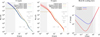 |
Fig. 11 Same as Fig. 6 for C- and S-types with a modified scaling law (“idea 2”). After this modification, both synthetic SFDs agree very well with the observed SFDs above the observational limits, and almost none “undershoots” the observed SFDs below the limits. The respective pseudo χ2 was 50.0. For reference, we also plot the corresponding best-fit scaling laws for the C- and S-types (Eqs. (3) and (4)) with the gray areas corresponding to the range of sizes below the observational limits. |
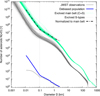 |
Fig. 12 Comparison of our collisional model with JWST observations (Burdanov et al. 2025). The SFD for the sum of C- and S-types (green) exhibits a change of slope from shallow to steep (q = −2.66) at approximately 100 m, in agreement with the observed (gray), debiased (blue), and scaled (dash-dotted) SFD from JWST. For reference, we also plot the synthetic SFD of S-types (gray); these S-types are about five times less numerous than C-types and exhibit a change of slope at a smaller size (∼50m). |
Acknowledgements
M.B. was supported by GACR grants nos. 25-16507S, 2516789S of the Czech Science Foundation. We thank the referee Rogerio Deienno for a constructive review, which helped us to clearly explain our results.
References
- Anders, E. 1965, Icarus, 4, 399 [Google Scholar]
- Anderson, S. E., Vernazza, P., & Brož, M. 2025, Nat. Astron., 9, 1464 [Google Scholar]
- Benz, W., & Asphaug, E. 1994, Icarus, 107, 98 [Google Scholar]
- Benz, W., & Asphaug, E. 1995, Comput. Phys. Commun., 87, 253 [NASA ADS] [CrossRef] [Google Scholar]
- Benz, W., & Asphaug, E. 1999, Icarus, 142, 5 [NASA ADS] [CrossRef] [Google Scholar]
- Binzel, R. P., DeMeo, F. E., Turtelboom, E. V., et al. 2019, Icarus, 324, 41 [Google Scholar]
- Blanton, M. R., Bershady, M. A., Abolfathi, B., et al. 2017, AJ, 154, 28 [Google Scholar]
- Borovicka, J., Popova, O., & Spurný, P. 2019, Meteor. Planet. Sci., 54, 1024 [Google Scholar]
- Bottke, W. F., & Greenberg, R. 1993, Geophys. Res. Lett., 20, 879 [Google Scholar]
- Bottke, W. F., Durda, D. D., Nesvorný, D., et al. 2005, Icarus, 175, 111 [Google Scholar]
- Bottke, William F. J., Vokrouhlický, D., Rubincam, D. P., & Nesvorný, D. 2006, Annu. Rev. Earth Planet. Sci., 34, 157 [CrossRef] [Google Scholar]
- Bottke, W. F., Brož, M., O’Brien, D. P., et al. 2015, in Asteroids IV, 701 [Google Scholar]
- Bottke, W., Walsh, K., Vokrouhlický, D., & Nesvorný, D. 2020a, in AAS/Division for Planetary Sciences Meeting Abstracts, 52, 402.02 [Google Scholar]
- Bottke, W. F., Vokrouhlický, D., Ballouz, R. L., et al. 2020b, AJ, 160, 14 [Google Scholar]
- Bottke, W., Vokrouhlický, D., Marschall, R., et al. 2022, in AAS/Division for Planetary Sciences Meeting Abstracts, 54, 304.03 [Google Scholar]
- Bowell, E., Hapke, B., Domingue, D., et al. 1989, in Asteroids II, eds. R. P. Binzel, T. Gehrels, & M. S. Matthews, 524 [Google Scholar]
- Brož, M., Ďurech, J., Carry, B., et al. 2022, A&A, 657, A76 [NASA ADS] [CrossRef] [EDP Sciences] [Google Scholar]
- Brož, M., Vernazza, P., Marsset, M., et al. 2024, A&A, 689, A183 [NASA ADS] [CrossRef] [EDP Sciences] [Google Scholar]
- Brož, M., Binzel, R., Vernazza, P., et al. 2026, A&A, in press https://doi.org/10.1051/0004-6361/202557980 [Google Scholar]
- Burdanov, A. Y., de Wit, J., Brož, M., et al. 2025, Nature, 638, 74 [Google Scholar]
- Bus, S. J., & Binzel, R. P. 2002a, Icarus, 158, 146 [Google Scholar]
- Bus, S. J., & Binzel, R. P. 2002b, Icarus, 158, 106 [CrossRef] [Google Scholar]
- Campo Bagatin, A., Cellino, A., Davis, D. R., Farinella, P., & Paolicchi, P. 1994, Planet. Space Sci., 42, 1079 [NASA ADS] [CrossRef] [Google Scholar]
- Capaccioni, F., Cerroni, P., Coradini, M., et al. 1986, Icarus, 66, 487 [Google Scholar]
- Čapek, D., & Vokrouhlický, D. 2004, Icarus, 172, 526 [Google Scholar]
- Carbognani, A. 2017, Planet. Space Sci., 147, 1 [Google Scholar]
- Cibulková, H., Brož, M., & Benavidez, P. G. 2014, Icarus, 241, 358 [CrossRef] [Google Scholar]
- Consolmagno, G., Britt, D., & Macke, R. 2008, Chem. Erde/Geochemistry, 68, 1 [NASA ADS] [Google Scholar]
- Cossins, P. J. 2010, arXiv e-prints [arXiv:1007.1245] [Google Scholar]
- Davis, D. R., Chapman, C. R., Greenberg, R., Weidenschilling, S. J., & Harris, A. W. 1979, in Asteroids, eds. T. Gehrels, & M. S. Matthews, 528 [Google Scholar]
- Davis, D. R., & Ryan, E. V. 1990, Icarus, 83, 156 [Google Scholar]
- Davis, D. R., Chapman, C. R., Weidenschilling, S. J., & Greenberg, R. 1985, Icarus, 62, 30 [NASA ADS] [CrossRef] [Google Scholar]
- Deienno, R., Nesvorný, D., Clement, M. S., et al. 2024, Planet. Sci. J., 5, 110 [Google Scholar]
- Deienno, R., Izidoro, A., Nesvorný, D., et al. 2025, ApJ, 986, 146 [Google Scholar]
- Delbo, M. 2004, PhD thesis, Free University of Berlin, Germany [Google Scholar]
- DeMeo, F. E., Binzel, R. P., Slivan, S. M., & Bus, S. J. 2009, Icarus, 202, 160 [Google Scholar]
- Dohnanyi, J. S. 1969, J. Geophys. Res., 74, 2531 [Google Scholar]
- Durda, D. D., Greenberg, R., & Jedicke, R. 1998, Icarus, 135, 431 [Google Scholar]
- Durda, D. D., Bottke, W. F., Nesvorný, D., et al. 2007, Icarus, 186, 498 [NASA ADS] [CrossRef] [Google Scholar]
- Ďurech, J., Sidorin, V., & Kaasalainen, M. 2010, A&A, 513, A46 [Google Scholar]
- Ďurech, J., Hanus, J., & Vanco, R. 2019, A&A, 631, A2 [Google Scholar]
- Fujiwara, A., Kamimoto, G., & Tsukamoto, A. 1977, Icarus, 31, 277 [NASA ADS] [CrossRef] [Google Scholar]
- Gallegos, C., Fuentes, C., & Peña, J. 2023, Planet. Sci. J., 4, 128 [Google Scholar]
- Gault, D. E., Moore, H. J., & Shoemaker, E. M. 1963, Spray Ejected from the Lunar Surface by Meteoroid Impact [Google Scholar]
- Gladman, B. J., Davis, D. R., Neese, C., et al. 2009, Icarus, 202, 104 [NASA ADS] [CrossRef] [Google Scholar]
- Gradie, J., & Tedesco, E. 1982, Science, 216, 1405 [NASA ADS] [CrossRef] [Google Scholar]
- Granvik, M., Morbidelli, A., Jedicke, R., et al. 2016, Nature, 530, 303 [Google Scholar]
- Greenberg, R. 1982, AJ, 87, 184 [Google Scholar]
- Hendler, N. P., & Malhotra, R. 2020, Planet. Sci. J., 1, 75 [Google Scholar]
- Hutchison, R. 2007, Cambridge Planetary Science: Meteorites: A Petrologic, Chemical and Isotopic Synthesis Series Number 2 (Cambridge, England: Cambridge University Press) [Google Scholar]
- Ivezić, Ž., Tabachnik, S., Rafikov, R., et al. 2001, AJ, 122, 2749 [Google Scholar]
- Jutzi, M. 2015, Planet. Space Sci., 107, 3 [CrossRef] [Google Scholar]
- Jutzi, M., Benz, W., & Michel, P. 2008, Icarus, 198, 242 [NASA ADS] [CrossRef] [Google Scholar]
- Jutzi, M., Michel, P., Benz, W., & Richardson, D. C. 2010, Icarus, 207, 54 [Google Scholar]
- Jutzi, M., Raducan, S. D., Landeck, A., Blum, J., & Michel, P. 2023, in LPI Contributions, 2851, Asteroids, Comets, Meteors Conference, 2439 [Google Scholar]
- Kirkwood, D. 1860, AJ, 6, 126 [Google Scholar]
- Knezevic, Z., & Milani, A. 2012, in IAU Joint Discussion, P18 [Google Scholar]
- Landgraf, M., Liou, J. C., Zook, H. A., & Grün, E. 2002, AJ, 123, 2857 [Google Scholar]
- Love, S. G., & Ahrens, T. J. 1996, Icarus, 124, 141 [Google Scholar]
- Macke, R. J., Consolmagno, G. J., & Britt, D. T. 2011, Meteor. Planet. Sci., 46, 1842 [Google Scholar]
- Maeda, N., Terai, T., Ohtsuki, K., et al. 2021, AJ, 162, 280 [NASA ADS] [CrossRef] [Google Scholar]
- Marchis, F., Jorda, L., Vernazza, P., et al. 2021, A&A, 653, A57 [NASA ADS] [CrossRef] [EDP Sciences] [Google Scholar]
- Marschall, R., Nesvorný, D., Deienno, R., et al. 2022, AJ, 164, 167 [NASA ADS] [CrossRef] [Google Scholar]
- Marsset, M., DeMeo, F. E., Burt, B., et al. 2022, AJ, 163, 165 [NASA ADS] [CrossRef] [Google Scholar]
- Marzari, F., Rossi, A., & Scheeres, D. J. 2011, Icarus, 214, 622 [NASA ADS] [CrossRef] [Google Scholar]
- Masiero, J. R., Mainzer, A. K., Grav, T., et al. 2011, ApJ, 741, 68 [Google Scholar]
- Michel, P., Benz, W., Tanga, P., & Richardson, D. C. 2001, Science, 294, 1696 [NASA ADS] [CrossRef] [Google Scholar]
- Morbidelli, A., Bottke, W. F., Nesvorný, D., & Levison, H. F. 2009, Icarus, 204, 558 [Google Scholar]
- Moskovitz, N. A., Wasserman, L., Burt, B., et al. 2022, Astron. Comput., 41, 100661 [NASA ADS] [CrossRef] [Google Scholar]
- Mothé-Diniz, T., Carvano, J. M. á., & Lazzaro, D. 2003, Icarus, 162, 10 [CrossRef] [Google Scholar]
- Nakamura, A., Suguiyama, K., & Fujiwara, A. 1992, Icarus, 100, 127 [Google Scholar]
- Nesvorný, D., Morbidelli, A., Vokrouhlický, D., Bottke, W. F., & Brož, M. 2002, Icarus, 157, 155 [Google Scholar]
- Nesvorný, D., Enke, B. L., Bottke, W. F., et al. 2006, Icarus, 183, 296 [Google Scholar]
- Nesvorný, D., Brož, M., & Carruba, V. 2015, in Asteroids IV, 297 [Google Scholar]
- Nesvorný, D., Roig, F. V., Vokrouhlický, D., et al. 2023, Icarus, 399, 115545 [CrossRef] [Google Scholar]
- Nesvorný, D., Vokrouhlický, D., Shelly, F., et al. 2024, Icarus, 417, 116110 [Google Scholar]
- O’Brien, D. P., & Greenberg, R. 2003, Icarus, 164, 334 [CrossRef] [Google Scholar]
- O’Brien, D. P., & Greenberg, R. 2005, Icarus, 178, 179 [CrossRef] [Google Scholar]
- Öpik, E. J. 1951, Proc. R. Irish Acad. Sect. A, 54, 165 [Google Scholar]
- Parker, A., Ivezić, Ž., Jurić, M., et al. 2008, Icarus, 198, 138 [Google Scholar]
- Rozehnal, J., Brož, M., Nesvorný, D., et al. 2022, Icarus, 383, 115064 [NASA ADS] [CrossRef] [Google Scholar]
- Rubincam, D. P. 2000, Icarus, 148, 2 [Google Scholar]
- Rubinstein, R. Y., & Kroese, D. P. 2016, Simulation and the Monte Carlo Method, 3rd edn., Wiley Series in Probability and Statistics (Nashville, TN: John Wiley & Sons) [Google Scholar]
- Schwartz, S. R., Yu, Y., Michel, P., & Jutzi, M. 2016, Adv. Space Res., 57, 1832 [Google Scholar]
- Ševeček, P., Brož, M., Nesvorný, D., et al. 2017, Icarus, 296, 239 [Google Scholar]
- Ševeček, P., Brož, M., & Jutzi, M. 2019, A&A, 629, A122 [Google Scholar]
- Shober, P. M., Devillepoix, H. A. R., Vaubaillon, J., et al. 2025, Nat. Astron., 9, 799 [Google Scholar]
- Tedesco, E. F., & Desert, F.-X. 2002, AJ, 123, 2070 [NASA ADS] [CrossRef] [Google Scholar]
- Tholen, D. J. 1984, PhD thesis, University of Arizona [Google Scholar]
- Vernazza, P., Brož, M., Drouard, A., et al. 2018, A&A, 618, A154 [NASA ADS] [CrossRef] [EDP Sciences] [Google Scholar]
- Vernazza, P., Ferrais, M., Jorda, L., et al. 2021, A&A, 654, A56 [NASA ADS] [CrossRef] [EDP Sciences] [Google Scholar]
- Vokrouhlický, D., Brož, M., Morbidelli, A., et al. 2006, Icarus, 182, 92 [CrossRef] [Google Scholar]
- Vokrouhlický, D., Bottke, W. F., Chesley, S. R., Scheeres, D. J., & Statler, T. S. 2015, in Asteroids IV, eds. P. Michel, F. E. DeMeo, & W. F. Bottke, 509 [Google Scholar]
- Vokrouhlický, D., Nesvorný, D., Bottke, W. F., & Morbidelli, A. 2010, AJ, 139, 2148 [CrossRef] [Google Scholar]
- Vávra, M. 2024, Master’s thesis, Charles University, Prague, Czech Republic [Google Scholar]
- Walsh, K. J., Richardson, D. C., & Michel, P. 2008, Nature, 454, 188 [Google Scholar]
- Walsh, K. J., Ballouz, R. L., Bottke, W. F., et al. 2024, Nat. Commun., 15, 5653 [Google Scholar]
- Warner, B. D., Harris, A. W., & Pravec, P. 2009, Icarus, 202, 134 [NASA ADS] [CrossRef] [Google Scholar]
- Yamauchi, C., Fujishima, S., Ikeda, N., et al. 2011, PASP, 123, 852 [Google Scholar]
- Zappalà, V., Cellino, A., Farinella, P., & Knezevic, Z. 1990, AJ, 100, 2030 [CrossRef] [Google Scholar]
- Zellner, B. 1979, in Asteroids, eds. T. Gehrels, & M. S. Matthews, 783 [Google Scholar]
Appendix A Note on the YORP effect
Alternatively, weakness at sub-kilometer sizes might be related to the YORP effect (Rubincam 2000). If bodies spin up over the spin barrier, they disrupt (Walsh et al. 2008; Marzari et al. 2011) and such disruptions are not accounted for in our model. However, the scaling of the YORP effect (Čapek & Vokrouhlický 2004) with the semimajor axis (a−2), the bulk density (ρ−1), suggests that C- and S-types should be comparable in this regard. Consequently, the differences between SFDs of C- and S-types should be attributed to something else.
Appendix B Note on the Yarkovsky effect
Alternatively, the deficiency of S-types at sub-km sizes might be related to the Yarkovsky drift (e.g., Vokrouhlický et al. 2015), or equivalently the decay timescales τmb. In principle, they might be different for C- and S-types. We constrained them by the debiased SFD of C- and S-type NEOs, as determined by Nesvorný et al. (2024). According to our collisional model, τmb for C-types should be substantially increased (by a factor of ≈10), but for S-types, which are more numerous among NEOs (Marsset et al. 2022), it was impossible to reach an equilibrium at the observed level.
In order to avoid this discrepancy, we adjusted the decay timescales τneo. For C-types, we decreased the value to 3 My, in agreement with dynamical simulations of NEOs originating from C-type families (Brož et al. 2024). For S-types, we increased the value up to 30 My, which is possible for long-lived objects among NEOs, originating preferentially from S-type families; the well-known example is (99924) Apophis (Brož et al. 2026). This solves the discrepancy; τmb for C-types is increased only by a factor of 2, and for S-types it is decreased by a factor of 2 (Fig. B.1), which is sufficient to reach the equilibrium of S-type NEOs. However, our collisional model also indicates that these adjustments further decreased the main-belt population of S-types, so their deficiency should be attributed to something else.
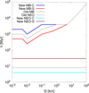 |
Fig. B.1 Decay timescales τmb and τneo of C- and S-types for our modified collisional model, aiming at fitting the SFDs of C- and S-type NEOs (Nesvorný et al. 2024). The new timescales are plotted in color, the old ones in gray. |
Appendix C Definition of χ2
For individual populations (C- or S-types), we define the contributions to χ2 as
 (C.1)
(C.1)
where N(≥Di)med is the median of the set  , whose members (labeled by k) are 100 individual evolved SFDs at size Di; N(≥ Di)obs is the observed SFD, and n is the number of individual bins (we chose n = 102). We assumed formal uncertainties σi ≡ 0.1 N(≥Di)obs, similarly as in Cibulková et al. (2014). The smallest size D1 corresponds to our estimate of the observational limit and the biggest size Dn to the maximum size for evaluating χ2. The bin size log [dD] in the log space is constant, therefore log [dD] = (log [Dn] - log [D1])/(n - 1). We finally evaluate the total χ2 as a sum for C- and S-types
 (C.2)
(C.2)
Since individual points in the evolved SFDs, as well as in the observed cumulative SFD, do not have exactly the same resolution in sizes, all  and N(≥Di)obs were interpolated linearly in the log-log plane.
Appendix D Algorithm for an assignment of C-and S-types
The algorithm, we implemented to assign C-, S-, or other types to each asteroid with unknown taxonomies is described as follows. The asteroid were identified in five catalogs, namely, Astorb (osculating orbital elements a, e, i and absolute magnitudes H, Moskovitz et al. 2022); Astdys (proper orbital elements ap, ep, ip, Knezevic & Milani 2012); AKARI (albedo pV, Yamauchi et al. 2011); WISE (albedo pV, Masiero et al. 2011) and SDSS (colours a* and i - z, Blanton et al. 2017). If pV was found in both AKARI and WISE, we preferred the one from AKARI.
We split asteroids into five groups, which differ from each other according to the knowledge of a*, i - z and pV. The most reliable asteroids are in the first group (I), as they have all three quantities known and all their uncertainties are below 0.1. The second (II) has at least one uncertainty above 0.1. The third (III) has only a* and i - z known, the fourth (IV) has only pV known and the fifth (V) has all three quantities unknown.
We then computed the individual distributions dN for our control sample of C- or S-types and for individual quantities (a*, i - z and pV). We assumed each quantity is normally distributed, thus the formula is
![Mathematical equation: \dd N(x)=\sum_{i=1}^n \frac{1}{\sqrt{2\pi}\sigma_i}\exp[-\,\frac{1}{2}\left(\frac{x-q_i}{\sigma_i}\right)^2],](/articles/aa/full_html/2026/03/aa57725-25/aa57725-25-eq11.png) (D.1)
(D.1)
where the summation is performed over all asteroids in either C- (n = 56) or S-type (n = 72) control sample; qi is the specific value of quantity of i-th asteroid and σi is its uncertainty; x is the independent variable where the distribution is evaluated. We denote these control-sample distributions with sub- and superscripts to distinguish C- and S-types as well as individual quantities, for example,  .
.
For an asteroid with unknown taxonomy, we assumed that individual quantities are also normally distributed, for example, for the albedo
![Mathematical equation: G_{pV}(x)\equiv\frac{1}{\sqrt{2\pi}\sigma_{\!pV}}\exp[-\frac{1}{2}\left(\frac{x-pV}{\sigma_{\!pV}}\right)^2]\,.\label{G}](/articles/aa/full_html/2026/03/aa57725-25/aa57725-25-eq13.png) (D.2)
(D.2)
The five groups are inspected asteroid by asteroid, separately in the inner, middle, and outer parts of the MB. If an asteroid was present in the SMASSII database (Bus & Binzel 2002a), its taxonomy was directly assigned (C-, S- or other types). If not present, the observed distributions of our control samples (Figs. 1, 2) and the distributions defined in Eq. (D.2) were used to assign taxonomy. The way of assignment differs for different groups:
-
The quantity Ctot is calculated as the product of three integrals
 (D.3)
(D.3)and similarly Stot. If Ctot < 0.1 and Stot < 0.1, then other taxonomy is assigned. Else a pseudo-random number r between 0 and 1 is generated and if
 (D.4)
(D.4)then C-type is assigned, else S-type is assigned. If the assigned taxonomy is C/S/other, then the tuple of asteroid’s a*, σa*, i - z, σi-z, pV, σpV is appended to a set denoted as C/S/O.
Same as in the previous group. However, now and in the following, a*, i - z, pV, σa*, σi-z, σpV is not appended to the sets C, S or O.
Ctot and Stot are calculated as the product of the first two integrals in Eq. (D.3). If Ctot < 0.12/3 and Stot < 0.12/3, then other taxonomy is assigned. Else, the pseudo-random number generator is called and the inequality Eq. (D.4) is tested again. If assigned taxonomy is C/S/other, then pV and it’s corresponding uncertainty σpV is randomly chosen from the set C/S/O. The size D is calculated according to Eq. (1).
Ctot and Stot are calculated with the last integral in Eq. (D.3). If Ctot < 0.11/3 and Stot < 0.11/3, then other taxonomy is assigned. Else, again, a pseudo-random number generator is called. If assigned taxonomy is C/S/other, then the tuple of a*, i - z, σa* and σi-z is randomly chosen from the set C/S/O.
The tuple of a*, σa*, i - z, σi-z, pV and σpV is randomly chosen from the union of the sets C, S and O and the size D is calculated according to Eq. (1). The assigned taxonomy is C/S/other if the tuple is chosen from the set C/S/O.
Appendix E Supplementary tables
Collisional probabilities p and impact velocities vimp between different populations. The value of the uncertainty corresponds to the uncertainty of the mean.
Appendix F Supplementary figures
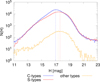 |
Fig. F.1 The differential distribution of absolute magnitude H with binning dH = 0.1 mag for C- (blue), S- (red) and other types (orange). The positions of Hmax of individual distributions are highlighted by vertical dotted lines - blue for C-, red for S-, and orange for other types. |
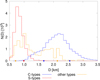 |
Fig. F.2 The differential SFDs with binning dD = 0.1 km for C- (blue), S- (red), and other types (orange) within the most populated absolute magnitude bin. The blue (for C-), red (for S-) and orange (for other types) points correspond to the borders of size ranges within the observational limit sizes lie. The lower bound of S- and other types is the same, therefore the lower bound of S-types is not visible. |
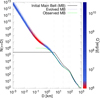 |
Fig. F.3 The first type of the initial size-frequency distribution (SFD) (black line), 100 evolved (synthetic) SFDs (color lines) and the observed SFD (green line) of the whole MB population. The strength Q*(D) (scaling law) is highlighted by the color bar, emphasized in the vicinity of the minimum (red color). |
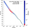 |
Fig. F.4 Same as Fig. F.3, computed for the second type of initial SFD. The slopes between 4 and 15 km as well as below 0.1 km, i.e., −2.5, correspond to the Dohnanyi (1969) equilibrium slope. |
 |
Fig. F.6 Six and three trial initial SFDs of C- and S-types (gray), compared to the original ones (black). The pair of C- (blue) and S-types (red) initial SFDs, which resulted in the lowest χ2, is also plotted. |
All Tables
Collisional probabilities p and impact velocities vimp between different populations. The value of the uncertainty corresponds to the uncertainty of the mean.
All Figures
|
Fig. 1 Scatter plot of the C- (blue) and S-type (red) control samples in the i - z vs. a* plane, along with their uncertainties σi-z and σa*. |
| In the text | |
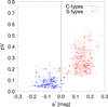 |
Fig. 2 Same as Fig. 1, but in the pV vs. a* plane. |
| In the text | |
|
Fig. 3 Scatter plot of eccentricity vs. semimajor axis (both proper or osculating) for all resulted 601 213 C-, 453 998 S-, and 9823 other types across different parts of the MB (inner, middle, and outer) separated by vertical black lines. Above the plot are the relative numbers of each taxonomy (blue for C-, red for S-, and orange for other types) within the specific parts of the MB. |
| In the text | |
|
Fig. 4 Observed SFD of the entire MB (green) and its individual parts: inner (red), middle (magenta), and outer (blue). We highlight the three largest asteroids in each region: inner - (19) Fortuna, (7) Iris, and (4) Vesta (red points); middle - (15) Eunomia, (2) Pallas, and (1) Ceres (magenta points); and outer - (704) Interamnia, (52) Europa, and (10) Hygiea (blue points). The “star-shaped” points on each SFD mark the limit size ranges obtained in Sect. 2.3, below which the data are observationally incomplete for the entire MB (green), inner (red), middle (magenta), and outer (blue) parts. The observed SFDs differ significantly, even above 100 km, where collisional evolution is negligible, implying different initial conditions. |
| In the text | |
|
Fig. 5 Same as Fig. 4, but for C-types (blue), S-types (red), and other types (orange). We include: the five largest C-types - (1) Ceres, (10) Hygiea, (52) Europa, (511) Davida, and (31) Euphrosyne (blue points); S-types - (15) Eunomia, (7) Iris, (3) Juno, (532) Herculina, and (29) Amphitrite (red points); and other types (4) Vesta, (2) Pallas, (704) Interamnia, (65) Cybele, and (87) Sylvia (orange points). |
| In the text | |
|
Fig. 6 Initial SFD (black), 100 evolved SFDs of the inner (red), middle (pink), and outer (blue) parts, and their respective observed SFD (green). The vertical dashed gray lines represent size ranges where the initial SFD was approximated by a different power law, i.e., a different slope. For the inner part, for example, the slopes are −3.55 above 100 km, −2.30 between 100 and 60 km, −1.65 between 60 and 15 km, and −4.00 between 15 and 3 km. The last slope below 3 km was set to zero, i.e., a constant cumulative SFD (“no tail”). Individual slopes are shown in gray within the panels at the respective size ranges. Density ρ, normalization size dnorm, and the normalization number nnorm for each part are shown on the right side of the respective panel. The gray areas correspond to the size ranges below the observational limits. The problem in the inner part is that most evolved SFDs lie below the observed SFD below D ~ 3 km. |
| In the text | |
|
Fig. 7 Same as Fig. 6 for the C-types, S-types, and other types. The problem with both C- and S-types is that most evolved SFDs lie below the observed SFD below D ~ 7 and 4 km, respectively. Conversely, evolved SFDs of other types always lie above the observed SFD (see text for discussion). |
| In the text | |
|
Fig. 8 Original scaling law (gray) and its modifications (labeled here as “ideas”), plotted in blue, pink, red, and orange. |
| In the text | |
|
Fig. 9 Twelve scaling laws (gray) tested for the inner belt, compared to the original (black) from Sect. 3.5. Those, which substantially increased the evolved SFDs below the observational limit, are shown in red and orange. The directions of scaling law minimum changes for decreasing a and D0 are shown by red and orange arrows, respectively. |
| In the text | |
|
Fig. 10 Same as Fig. 6, for the inner part and a modified scaling law (“idea 2”). For comparison, we also plot SFDs for the original scaling law (gray lines, corresponding to the left panel in Fig. 6). The synthetic SFDs of the middle and outer belt did not change considerably. |
| In the text | |
|
Fig. 11 Same as Fig. 6 for C- and S-types with a modified scaling law (“idea 2”). After this modification, both synthetic SFDs agree very well with the observed SFDs above the observational limits, and almost none “undershoots” the observed SFDs below the limits. The respective pseudo χ2 was 50.0. For reference, we also plot the corresponding best-fit scaling laws for the C- and S-types (Eqs. (3) and (4)) with the gray areas corresponding to the range of sizes below the observational limits. |
| In the text | |
|
Fig. 12 Comparison of our collisional model with JWST observations (Burdanov et al. 2025). The SFD for the sum of C- and S-types (green) exhibits a change of slope from shallow to steep (q = −2.66) at approximately 100 m, in agreement with the observed (gray), debiased (blue), and scaled (dash-dotted) SFD from JWST. For reference, we also plot the synthetic SFD of S-types (gray); these S-types are about five times less numerous than C-types and exhibit a change of slope at a smaller size (∼50m). |
| In the text | |
|
Fig. B.1 Decay timescales τmb and τneo of C- and S-types for our modified collisional model, aiming at fitting the SFDs of C- and S-type NEOs (Nesvorný et al. 2024). The new timescales are plotted in color, the old ones in gray. |
| In the text | |
|
Fig. F.1 The differential distribution of absolute magnitude H with binning dH = 0.1 mag for C- (blue), S- (red) and other types (orange). The positions of Hmax of individual distributions are highlighted by vertical dotted lines - blue for C-, red for S-, and orange for other types. |
| In the text | |
|
Fig. F.2 The differential SFDs with binning dD = 0.1 km for C- (blue), S- (red), and other types (orange) within the most populated absolute magnitude bin. The blue (for C-), red (for S-) and orange (for other types) points correspond to the borders of size ranges within the observational limit sizes lie. The lower bound of S- and other types is the same, therefore the lower bound of S-types is not visible. |
| In the text | |
|
Fig. F.3 The first type of the initial size-frequency distribution (SFD) (black line), 100 evolved (synthetic) SFDs (color lines) and the observed SFD (green line) of the whole MB population. The strength Q*(D) (scaling law) is highlighted by the color bar, emphasized in the vicinity of the minimum (red color). |
| In the text | |
|
Fig. F.4 Same as Fig. F.3, computed for the second type of initial SFD. The slopes between 4 and 15 km as well as below 0.1 km, i.e., −2.5, correspond to the Dohnanyi (1969) equilibrium slope. |
| In the text | |
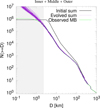 |
Fig. F.5 Summed SFDs of all three parts from Fig. 6. |
| In the text | |
|
Fig. F.6 Six and three trial initial SFDs of C- and S-types (gray), compared to the original ones (black). The pair of C- (blue) and S-types (red) initial SFDs, which resulted in the lowest χ2, is also plotted. |
| In the text | |
Current usage metrics show cumulative count of Article Views (full-text article views including HTML views, PDF and ePub downloads, according to the available data) and Abstracts Views on Vision4Press platform.
Data correspond to usage on the plateform after 2015. The current usage metrics is available 48-96 hours after online publication and is updated daily on week days.
Initial download of the metrics may take a while.