| Issue |
A&A
Volume 707, March 2026
|
|
|---|---|---|
| Article Number | A60 | |
| Number of page(s) | 17 | |
| Section | Planets, planetary systems, and small bodies | |
| DOI | https://doi.org/10.1051/0004-6361/202557819 | |
| Published online | 04 March 2026 | |
Transit distances and compositions of low-velocity exocomets in the β Pic system
Institut d’Astrophysique de Paris, CNRS, UMR 7095, Sorbonne Université, 98 bis boulevard Arago,
75014
Paris,
France
★ Corresponding author: This email address is being protected from spambots. You need JavaScript enabled to view it.
Received:
24
October
2025
Accepted:
21
January
2026
Abstract
Beta Pictoris is a young nearby A5V star, about 20 Myr old, that is embedded in a prominent debris disc. For the past 40 years, variable absorption features, produced by the gaseous tails of exocomets transiting the star, have been observed in the stellar spectrum. Yet, despite the large number of observations available, the origin and dynamical evolution of the exocomets remain poorly understood. Here we present new spectroscopic observations of β Pic obtained on April 29, 2025, with the Hubble Space Telescope and the High Accuracy Radial Velocity Planet Searcher. We report the detection of three strong exocomet signatures at low radial velocities (−7.5, +2.5, and +10 km/s) from a large set of lines from various species and excitation levels. We show that the three exocometary tails have different excitation states, indicating that they are located at different distances from the star. Using a detailed modelling of the excitation state of the transiting gas, which includes both radiative and collisional excitation, we derived the transit distance of the three exocometary gaseous tails to be 0.88 ± 0.08, 4.7 ± 0.3, and 1.52 ± 0.15 au. These values are much larger than previous estimates, which generally placed the transient features within 0.2 au. This reveals that gaseous tails produced by exocomets sublimating close to the star can expand and migrate over large distances while still remaining detectable in absorption spectroscopy. Our study provides a new method for measuring the transit distance of exocomets based on excitation modelling; this complements the acceleration method, which is only applicable to high-velocity objects.
Key words: techniques: spectroscopic / comets: general / stars: individual: Beta Pic
© The Authors 2026
 Open Access article, published by EDP Sciences, under the terms of the Creative Commons Attribution License (https://creativecommons.org/licenses/by/4.0), which permits unrestricted use, distribution, and reproduction in any medium, provided the original work is properly cited.
This article is published in open access under the Subscribe to Open model. This email address is being protected from spambots. You need JavaScript enabled to view it. to support open access publication.
1 Introduction
Beta Pictoris (β Pic) is a young (20 Myr; Miret-Roig et al. 2020), nearby (19.3 pc; Crifo et al. 1997) A5V star that hosts a complex extrasolar system. The star is surrounded by a prominent debris disc seen edge-on; this disc expands over hundreds of astronomical units (Smith & Terrile 1984; Lecavelier des Etangs et al. 1993) and is composed of dust (Apai et al. 2015; Rebollido et al. 2024) and volatile-rich gas (Roberge et al. 2000; Dent et al. 2014; Brandeker et al. 2016). The system also hosts two massive planets, β Pic b (Lagrange et al. 2010) and β Pic c (Lagrange et al. 2019; Nowak et al. 2020), orbiting at 2.7 and 9 au, whose presence was initially predicted from the disc morphology (e.g. Heap et al. 2000; Okamoto et al. 2004). Recent observations with JWST have shown evidence of a recent (~100 yr) collision between large planetesimals at ~100 au from β Pic (Chen et al. 2024; Rebollido et al. 2024), hinting that the system is still rapidly evolving.
In addition to its disc and planets, β Pic is widely known for harbouring a unique system of extrasolar comets, or exocomets, which are analogues of comets in our own Solar System. These objects are detected when their tails, composed of dust and gas, transit the star and produce absorption signatures in the stellar spectrum (e.g. Ferlet et al. 1987; Vidal-Madjar et al. 1994; Lagrange et al. 1995) or the star’s light curve (Zieba et al. 2019; Pavlenko et al. 2022; Lecavelier des Etangs et al. 2022). While signatures of such objects have been detected in other systems, such as HD 172555 (Kiefer et al. 2014a) and 49 Cet (Miles et al. 2016), β Pic stands out due to the intensity of its cometary activity. On average, each optical β Pic spectrum in the Ca II H&K lines shows six signatures of individual exocomets and, as of now, thousands of such objects have been detected, mostly using the Ca II doublet (Kiefer et al. 2014b). The complexity of the system, combined with the close proximity of the star and the favourable orientation of the disc, makes β Pic a unique laboratory for studying the last stages of planetary formation.
Many efforts have been devoted to studying the orbital dynamics of β Pic exocomets. Using the extensive set of observations obtained with the High Accuracy Radial Velocity Planet Searcher (HARPS) spectrograph, Kiefer et al. (2014b) showed that the comets can be divided into two broad dynamical families: the S family (for ‘shallow’), which produces faint and wide absorption features at high velocities (typically from −50 to more than +100 km/s), and the D family (‘deep’), which produces narrow and deep features at lower velocities (−10 to +30 km/s). Kiefer et al. (2014b) showed that the S and D families can be distinguished by the depth of their absorption in the Ca II K line, with D-family comets producing absorptions deeper than 40%. Based on the hydrodynamical model of Beust & Tagger (1993), Kiefer et al. (2014b) also inferred the typical transit distances of exocomets from the two families, finding 10 ± 3 R⋆ (0.07 ± 0.02 au) for the S family and 19 ± 4 R⋆ (0.14 ± 0.03 au) for the D family. These distances are much shorter than the typical periastron distances of the brightest comets in the Solar System (e.g. 0.91 au for Hale-Bopp). They are, however, consistent with the large amounts of refractory ions (Fe+, Ca+, etc) found in β Pic exocomets’ gaseous tails (e.g. Vrignaud et al. 2024), which are released by the sublimation of dust grains only at stellocentric distances below a few tens of stellar radii (for instance, Beust et al. 1996 provide a sublimation distance of 35 R⋆ = 0.25 au for tektite glass).
Directly measuring the transit distance (and, more generally, the orbital elements) of exocomets is a difficult task. Based on the acceleration of exocomet signatures in Ca II lines, Kennedy (2018) was able to measure the transit distance of a few β Pic exocomets. All the studied objects were found to transit below 20 R⋆ (0.14 au), in agreement with Kiefer et al. (2014b). More recently, Vrignaud & Lecavelier des Etangs (2024) showed that the excitation state of Fe II in β Pic exocomets is primarily set by the stellar radiation, and is therefore a direct probe of the distance to the star. Applying this principle to an exocomet with a radial velocity (RV) of ~30 km/s observed with the Hubble Space Telescope (HST), Vrignaud & Lecavelier des Etangs (2024) showed that the comet transited at less than 60 R⋆ (0.4 au), similar to the objects studied in Kennedy (2018).
However, as of now, all the exocomets that have had their transit distance directly measured (Kennedy 2018; Vrignaud & Lecavelier des Etangs 2024) belong to the S family. This is because S-family comets exhibit more isolated signatures and higher accelerations, owing to their closer proximity to β Pic. In contrast, the properties of D-family comets remain poorly constrained. Their absorption signatures are frequently blended and overlap with the stable circumstellar disc absorption (see e.g. Kiefer et al. 2014b), making them much more difficult to analyse. As a result, no direct constraints on the dynamical properties of the D family currently exist. Their transit distances (19 ± 4, R⋆) were inferred indirectly by Kiefer et al. (2014b) using the dynamical model of Beust & Tagger (1993). More recently, Beust et al. (2024) showed that the low RVs of D-family comets are consistent with an origin close to β Pic (0.5–1.2 au), where bodies can fall into high-order mean-motion resonances with β Pic c.
The goal of the present study is to directly constrain the orbital properties of D-family comets using spectroscopic observations obtained with the HST in 2025. These observations cover numerous UV Fe II lines spanning a wide range of excitation levels, which can be used as a probe of the transit distance of exocometary tails (Vrignaud & Lecavelier des Etangs 2024). The paper is organised as follows. In Sect. 2 we present our spectroscopic observations and the three exocomets under study. Then, in Sects. 3 and 4 we describe our approach to modelling the absorption spectra of the transiting exocomets and fit our spectroscopic data. Finally, in Sect. 5 we report our measurements of the transit distances and compositions of the studied exocomets, and we discuss the implication for the dynamical evolution of exocometary tails in the β Pic system.
Log of the β Pic spectra obtained on April 29, 2025.
2 Description of the observations
2.1 Studied spectrum
Spectroscopic observations of β Pic were obtained on April 29, 2025, from three instruments: the Space Telescope Imaging Spectrograph (STIS) and the Cosmic Origin Spectrograph (COS) on board the HST (programme #115.282N, PI: T. Vrignaud), and the HARPS mounted on the 3.6 m telescope of the European Southern Observatory (programme #115.282N PI: T. Vrignaud). A summary of the observations used in the present study is provided in Table 1, and the full spectrum is shown in Fig. 1.
The studied dataset covers almost the whole wavelength range from 1000 to 7000 Å. Specifically, the COS spectrum covers the 1100–1500 Å range, the six STIS spectra cover the 1500–2900 Å range, and the HARPS spectrum covers the 3800–6900 Å range. Altogether, they provide access to a large range of spectral lines (e.g. Fe I, Fe II, Ca II, Al III, C I, and C II), allowing for a detailed analysis of the physical and chemical properties of the circumstellar gas occulting the star. Simultaneous observations of such a large number of chemical species in the β Pic system are unprecedented.
The present analysis is based on the 1D extracted orders from the six STIS spectra (25–65 orders per spectrum), and the two spectral segments from the COS observations. For HARPS, we used the merged 1D spectrum (in which all spectral orders were resampled on a unique wavelength grid), summed over the full 2.25-hour observing sequence (27 exposures of 300 s each). The wavelengths table of the studied spectra were shifted to the β Pic rest frame, assuming a RV of 20.5 km/s (Brandeker 2011). In the following, all RVs will be expressed in β Pic rest frame.
Little reduction was applied to our dataset. The six STIS spectra, which partly overlap, were all re-normalised to a common flux level, using a procedure similar to that described in Sect. 2 of Vrignaud et al. (2024). This method consists in interpolating each individual spectrum with a cubic spline, calculated on spectral regions free of circumstellar and interstellar absorption. Each spectrum is then divided by its corresponding spline, which mitigates the effects of flux calibration variations from one exposure to another.
2.2 Overview of the detected signatures
A sample of the reduced STIS spectra obtained on April 29, 2025, is provided in Fig. 2 around two Fe II lines. For comparison, we also show archival STIS spectra of β Pic obtained between 1997 and 2018, as well as an estimate of the β Pic spectrum free of circumstellar absorption (black), reconstructed using all archival observations. The April 29, 2025, spectrum displays many absorption features, which we associate with three types of objects:
Low-velocity comets (LVCs), which produce deep and narrow absorption lines at RVs below 15 km/s. The April 29, 2025, spectrum shows three signatures from LVCs, around −7.5, +2.5 and +10 km/s (see Fig. 2). We associate these objects with the D family of Kiefer et al. (2014b).
High-velocity comets (HVCs), which produce shallow and broad absorption features at higher velocities (typically from about −100 km/s to more than +100 km/s). Several HVCs are detected in the April 29, 2025, spectrum, particularly around −50 km/s and +30 km/s (see Fig. 2). These objects have the typical characteristics of the S family (Kiefer et al. 2014b).
The circumstellar disc, which produces a narrow and stable signature at 0 km/s. Since the disc is located further out, it is primarily detected in the lines from the ground state level (see Sect. 2.3).
The HVCs seen in the April 29, 2025, spectrum resemble the exocomet signature observed on December 6, 1997, and studied in Vrignaud & Lecavelier des Etangs (2024). The transit distance of this previous comet was found to be below 0.4 au, based on the excitation state of Fe II in the gaseous tail. Given the similarity between this previously studied signature and the HVCs observed in the April 29, 2025, spectrum, it is likely that the latter are also produced by gaseous tails at short stellar distances, typically well below 1 au.
Low-velocity comets, however, are more difficult to interpret. Previous studies (e.g. Beust et al. 1998; Tobin et al. 2019; Hoeijmakers et al. 2025) showed that these features are fairly different from HVCs: they are much less time-variable (typically lasting for several days), do not show any acceleration (e.g. Kennedy 2018) and have much narrower absorption lines, with typical width of 1–5 km/s. The goal of the present study is to investigate the physical properties of these transiting components, using the spectrum obtained on April 29, 2025.
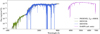 |
Fig. 1 Spectroscopic observations of β Pic obtained on April 29, 2025. The HARPS spectrum is not flux-calibrated and was simply re-normalised to a flux level similar to that of the STIS data. Numerous saturated absorption lines are visible in the STIS and HARPS spectra, attributed to Si II, C I, Al II, Fe II, Mg II, and Ca II. The HST spectra are consistent with a stellar model from the PHOENIX library (thick grey line; Husser et al. 2013) at Teff = 8000 K (see Sect. 4.1). |
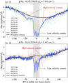 |
Fig. 2 Zoomed-in view of the STIS spectra of β Pic from April 29, 2025, around two Fe II lines. Top: view of the strong Fe II line at 2756.5 Å. Archival STIS spectra of β Pic covering the same line are shown in transparent font. The solid black line represents an estimate of the stellar photospheric continuum, free of circumstellar absorption. Bottom: same view of the shallower Fe II line at 2578.7 Å. This wavelength region is covered by two orders of the STIS echelle spectrograph. Since these two lines arise from excited states of Fe+, they do not show any signature of the circumstellar disc (see Sect. 2.3). |
2.3 The low-velocity comets of April 29, 2025
The April 29, 2025, spectrum shows absorption signatures from three strong LVCs (see Fig. 2). These LVCs are consistently detected in lines of Fe II, S I, Ni II, Cr II, Mn II, Si II (STIS and COS data), and Ca II (HARPS data). Their signatures also seem to be present in C I, Al II, and Mg II (STIS), also these lines are much harder to interpret due to their extreme saturation. Faint signatures may also be present in Zn II, Co II, and Sr II.
To isolate the absorption spectra of these LVCs, we constructed a reference spectrum free of their absorption. This reference spectrum was computed using a cubic spline interpolation across the full STIS, COS, and HARPS datasets, excluding all wavelength bins located within 20 km/s of any line where absorption from the LVCs is expected. The list of lines considered in this calculation was obtained through the following procedure: for all the species listed above (Fe II, Ni II, etc), we identified a set of metastable states with clear signatures from the LVCs (for instance, the 8 lowest levels of Ni II). For each of these metastable states, we then selected all lines with large oscillator strengths (typically >0.01). The 20 km/s threshold was chosen because signatures from the three LVCs are confined within the [−20,+20] km/s range for all the detected lines.
This reference spectrum is shown on Figs. 3 and 4 around several Fe II, Ni II and Si II lines. We emphasise that it is not intended to represent the stellar photospheric continuum, as it remains polluted by broad absorption features from HVCs. Instead, the goal of this reference spectrum is to estimate what the April 29, 2025, β Pic spectrum would look like without the three LVCs. The absorption spectrum of the three LVCs alone is obtained by taking the ratio of the observed spectrum to this reference.
The velocities of the three LVCs are identified with red ticks on Figs. 3 and 4. Following the nomenclature introduced in Lecavelier des Etangs et al. (2026), we designate these comets as C20250429a, C20250429b, and C20250429c. For brevity, we refer to them hereafter as LVCs #1, 2, and 3. LVC #1 is centred around −7.5 km/s, LVC #2 around 2.5 km/s, and LVC #3 around 10 km/s. A first look at the Fe II and Ni II signatures of the three LVCs reveals differences in their excitation states. Lines arising from low-excitation levels show a strong contribution from LVC #2 (centred around ≃2.5 km/s) compared to LVCs #1 and #3. In contrast, lines from highly excited levels show a very strong signature from LVC #1 (see the bottom panel of Fig. 3). Since the excitation state of exocometary tails is primarily controlled by the local radiation flux, and thus by the distance to the host star (Vrignaud & Lecavelier des Etangs 2024), this suggests that the three LVCs are located at different distances from β Pic. Specifically, LVC #1 seems to be rather close to the star (given the presence of excited Fe II levels), while LVC #2 appears to be further out. The goal of the remainder of this work is to quantify this general picture.
In addition to the three LVCs, Figs. 3 and 4 show the presence of an additional narrow absorption feature centred around 0 km/s. Among the lines shown in these figures, this central component is only detected in the Fe II λ2260 Å and Si II λ1808 Å lines arising from the ground states of Fe II and Si II (El=0 cm−1), and in the Ni II λ2223 Å line arising from the metastable state at El=8394 cm−1. This signature is naturally associated with the circumstellar disc surrounding β Pic. It is detected in the ground state of all atomic and ionised species (e.g. S I, Fe II, Ni II, Cr II, and Si II), as well as in the El=8394 cm−1 metastable state of Ni II, which has a long radiative lifetime. As discussed below, the weaker excitation of the disc is explained by its large distance to β Pic and to its low density, which limit the rates of radiative and collision excitation.
3 Modelling the low-velocity comets’ and disc’s absorptions
3.1 Principle
The various absorption features detected in the April 29, 2025, observations offer a favourable configuration for analysis: the three LVCs are spectrally resolved, and since none of them peaks around 0 km/s, the contribution from the circumstellar disc can also be isolated. The goal of the following sections is to build a model of the absorption spectra of these four components (the three LVCs and the disc), and to fit this model to the spectra obtained on April 29, 2025, in order to infer their physical and chemical properties. To achieve this, we follow and extend the approach of Vrignaud & Lecavelier des Etangs (2024), who studied the excitation state of Fe II in a β Pic exocomet. Contrary to this previous study, here we aim to directly fit the observed spectra of the transiting components rather than their excitation diagrams. This will allow us to rigorously account for the blending between the absorption signatures of the four components, the instrumental spectral dispersion, and the mixing of closely spaced multiplets.
With the goal of modelling each transiting component using the simplest possible parameterisation, we assume that each component lies at a unique distance d to β Pic and is characterised by a unique electronic temperature Te and electronic density ne (since the tails are ionised, electrons are considered the main collision partner). The line profile of each component is described by a Voigt profile, with a central velocity v and a Doppler broadening parameter b. We also assume that the studied species are well mixed within each component, due to efficient momentum transfer between ions through Coulomb interactions (Beust et al. 1989; Vrignaud et al. 2025). This assumption is supported by the similarity of the line profile observed in different species, and by the quasi-solar composition found in all transiting components (see Sect. 6.2).
 |
Fig. 3 Zoomed-in view of the STIS spectra of β Pic obtained on April 29, 2025, around four Fe II lines arising from different excitation levels. Errors bars were tabulated from the STIS data reduction pipeline. Red ticks indicate the velocities of the three main LVCs. The circumstellar disc (green tick, 0 km/s) is detected in the ground state of Fe II. Note that the λλ2260 and 2622 Å lines are covered by two spectral orders. |
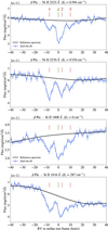 |
Fig. 4 Same as Fig. 3 but for two Ni II lines and two Si II lines. The disc is detected in the metastable state of Ni II at 8393 cm−1, and in the ground state of Si II. |
3.2 Self-absorption inside the gaseous clouds
As many lines in our spectrum are found to be highly saturated (most notably Fe II, Ni II, and Si II), we also take the self-absorption of the transiting objects into account. To do so, each component is divided into a finite number of gas bins (typically ~10–30), each containing an equal fraction of the total column density. These bins are arranged sequentially along the line of sight such that the first bin is fully exposed to the stellar flux, while each subsequent bin receives a progressively attenuated flux due to absorption from the preceding bins. The transmitted spectrum is calculated as follows:
We start by considering the first bin of the innermost component, directly exposed to the stellar flux. For all the studied species, we computed the level populations by solving the statistical equilibrium, taking into account both radiative and collisional excitation.
Using a comprehensive list of spectral lines from all the studied species and the computed level populations, we calculate the flux transmitted by the first bin. This flux is then passed to the second bin, located just behind the first, which thus receives a slightly weaker radiation field.
The statistical equilibrium of the second bin is then solved, using the absorbed stellar spectrum. We compute its transmitted flux, which in turn becomes the input for the third bin. This process is repeated iteratively across all bins of all gaseous components, which are processed by increasing distance from the star.
After all components have been considered, the last transmitted flux can be compared to our observations to constrain the physical parameters of the transiting gas clouds.
In the following, each transiting component is discretised into a number of gas bins chosen such that each bin has a Fe II column density of 2 × 1013 cm−2, except for the last bin. Since the Fe II column densities in our components range from 1.5 to 6 × 1014 cm−2 (see Sect. 5), this results in a reasonable number of 10–30 gas bins per component. The full model is computed in ~1 s on a single CPU.
3.3 Statistical equilibrium
To calculate the model spectrum, the statistical equilibrium needs to be computed in each bin of the transiting clouds.
Let us consider a gaseous component located at a distance d from the star, characterised by an electronic density ne and an electronic temperature Te. For any excitation level i of any atom or ion X, the statistical equilibrium equation is expressed as
![Mathematical equation: $\[\frac{\mathrm{d} n_i}{\mathrm{~d} t}=0,\]$](/articles/aa/full_html/2026/03/aa57819-25/aa57819-25-eq1.png)
where ni is the population of level i. Taking into account all radiative and collisional exchanges with other levels j ≠ i, this reads (Vrignaud & Lecavelier des Etangs 2024)
![Mathematical equation: $\[\begin{aligned}& \sum_{j<i}\left(C_{j i} n_e n_j-C_{i j} n_e n_i+B_{j i} \overline{J}_{i j} n_j-B_{i j} \overline{J}_{i j} n_i-A_{i j} n_i\right) \\+ & \sum_{j>i}\left(C_{j i} n_e n_j-C_{i j} n_e n_i+B_{j i} \overline{J}_{i j} n_j-B_{i j} \overline{J}_{i j} n_i+A_{j i} n_j\right)=0,\end{aligned}\]$](/articles/aa/full_html/2026/03/aa57819-25/aa57819-25-eq2.png) (1)
(1)
where Cij and Cji are the collisional excitation rates for the i → j and j → i transitions (which depend on the electronic density and temperature), Aji, Bij and Bji the Einstein coefficients for spontaneous decay, absorption and stimulated emission, and ![Mathematical equation: $\[\overline{J}_{i j}\]$](/articles/aa/full_html/2026/03/aa57819-25/aa57819-25-eq3.png) the line-averaged flux in the i ↔ j transition.
the line-averaged flux in the i ↔ j transition. ![Mathematical equation: $\[\overline{J}_{i j}\]$](/articles/aa/full_html/2026/03/aa57819-25/aa57819-25-eq4.png) is computed as
is computed as
![Mathematical equation: $\[\overline{J}_{i j}=\int_0^{+\infty} J_\nu \cdot \phi_{i j}(\nu) ~\mathrm{d} \nu,\]$](/articles/aa/full_html/2026/03/aa57819-25/aa57819-25-eq5.png) (2)
(2)
where ϕi,j is the line profile of the i ↔ j transition in the considered component and Jν the solid angle-averaged specific intensity at frequency ν:
![Mathematical equation: $\[J_\nu=\frac{1}{4 \pi} \int_{4 \pi} I_\nu \mathrm{~d} \Omega.\]$](/articles/aa/full_html/2026/03/aa57819-25/aa57819-25-eq6.png)
In the case of an optically thin medium, Jν is dominated by the stellar flux, and is thus given by ![Mathematical equation: $\[J_{\nu}=W ~I_{\nu}^{\star}\]$](/articles/aa/full_html/2026/03/aa57819-25/aa57819-25-eq7.png) , where
, where ![Mathematical equation: $\[W=\frac{1}{2}\left(1-\sqrt{1-\left(R_{\star} / d\right)^{2}}\right) \approx\left(\pi R_{\star}^{2}\right) /\left(4 \pi d^{2}\right)\]$](/articles/aa/full_html/2026/03/aa57819-25/aa57819-25-eq8.png) is the dilution factor and
is the dilution factor and ![Mathematical equation: $\[I_{\nu}^{\star}\]$](/articles/aa/full_html/2026/03/aa57819-25/aa57819-25-eq9.png) the average specific intensity of the stellar disc (unit: erg/s/cm2/Hz/sr). This approximation was used in Vrignaud & Lecavelier des Etangs (2024). In the present case, however, we choose to take self-absorption into account, by progressively reducing the radiation field going through the gas after it is absorbed (Sect. 3.2). The stellar flux (Jν) received by a gas bin is thus given by
the average specific intensity of the stellar disc (unit: erg/s/cm2/Hz/sr). This approximation was used in Vrignaud & Lecavelier des Etangs (2024). In the present case, however, we choose to take self-absorption into account, by progressively reducing the radiation field going through the gas after it is absorbed (Sect. 3.2). The stellar flux (Jν) received by a gas bin is thus given by
![Mathematical equation: $\[J_\nu=W I_\nu^{\star} ~e^{-\tau_\nu},\]$](/articles/aa/full_html/2026/03/aa57819-25/aa57819-25-eq10.png)
where τν is the optical thickness of the material occulting the current bin from the star. The corresponding line-integrated flux ![Mathematical equation: $\[\overline{J}_{i j}\]$](/articles/aa/full_html/2026/03/aa57819-25/aa57819-25-eq11.png) can be written as
can be written as
![Mathematical equation: $\[\overline{J_{i, j}}=\overline{J}_{i j, \text { abs }}^{\star}:=W \int_0^{+\infty} I_\nu^{\star} ~e^{-\tau_\nu} \cdot \phi_{i j}(\nu) ~\mathrm{d} \nu.\]$](/articles/aa/full_html/2026/03/aa57819-25/aa57819-25-eq12.png)
In addition, Eq. (1) neglects the possibility that photons produced by spontaneous emission are immediately reabsorbed by the surrounding gas when the cometary tail is optically thick. In this case, the excitation energy of a given ion is simply transferred to another particle, and the global level populations remain unchanged. This process is likely significant for the exocomets analysed in this work, whose signatures in Fe II or Si II lines are often strongly saturated. To account for this, we make use of the escape probability formalism, which consists in weighting the spontaneous decay rates Aijnj and Ajini, appearing in Eq. (1), by the probability that the emitted photon escapes the cloud in a single flight. To calculate this probability, we assume that the components have symmetric geometries relative to the line of sight, and that the transverse column densities Ntrans(X), taken from the cloud centre to their edge, are much smaller than the radial column densities N(X). For each component, we introduce a new parameter, f, defined as the ratio between the transverse and radial column density:
![Mathematical equation: $\[N_{\text {trans }}(X)=f \cdot N(X).\]$](/articles/aa/full_html/2026/03/aa57819-25/aa57819-25-eq13.png)
For the three LVCs, the escape probability of photons Pij in a given transition i ↔ j of species X is calculated assuming that the cometary tails have cylindrical, tube-like geometries. Integrating over all possible directions and frequencies, one finds
![Mathematical equation: $\[P_{i j}=\frac{1}{4 \pi} \int_0^\pi 2 \pi ~\sin (\theta) ~\mathrm{d} \theta \int_0^{+\infty} \phi_{i j}(\nu) \mathrm{d} \nu ~\exp \left(-\frac{\tau_{\text {trans }}(\nu)}{\sin (\theta)}\right),\]$](/articles/aa/full_html/2026/03/aa57819-25/aa57819-25-eq14.png)
where τtrans(ν) is the optical depth of the cloud at frequency v in the transverse direction, and θ is the angle between the line of sight symmetry axis and the escape direction. The optical depth τtrans(ν) is directly computed from the transverse column density Ntrans(X) and the level populations in the cloud, and thus depends on f.
For the disc, we adopt a slab geometry. The escape probability takes a slightly different form:
![Mathematical equation: $\[P_{i j}=\frac{1}{4 \pi} \int_0^\pi 2 \pi ~\sin (\theta) ~\mathrm{d} \theta \int_0^{+\infty} \phi_{i j}(\nu) ~\mathrm{d} \nu ~\exp \left(-\frac{\tau_{\text {trans }}(\nu)}{\cos (\theta)}\right),\]$](/articles/aa/full_html/2026/03/aa57819-25/aa57819-25-eq15.png)
where τtrans(ν) is here the optical depth of the disc at frequency v in the direction perpendicular to the disc plane, and is also computed from Ntrans(X).
Ultimately, the full statistical equilibrium equation used to calculate the level populations’ ni is given by
![Mathematical equation: $\[\begin{aligned}& \sum_{j<i}\left(C_{j i} n_e n_j-C_{i j} n_e n_i+B_{j i} \overline{J}_{i j, \text { abs}}^{\star} n_j-B_{i j} \overline{J}_{i j, \text { abs}}^{\star} n_i-P_{i j} A_{i j} n_i\right) \\+ & \sum_{j>i}\left(C_{j i} n_e n_j-C_{i j} n_e n_i+B_{j i} \overline{J}_{i j, \text { abs}}^{\star} n_j-B_{i j} \overline{J}_{i j, \text { abs}}^{\star} n_i+P_{i j} A_{j i} n_j\right) \\& =0.\end{aligned}\]$](/articles/aa/full_html/2026/03/aa57819-25/aa57819-25-eq16.png) (3)
(3)
In the model, each component is modelled with six global parameters, plus one column density per chemical species. The global parameters are the distance from the star (d); the electronic density (ne) and the electronic temperature (Te); the component velocity (v) and Doppler broadening parameter (b); and the ratio between the transverse and radial column densities (f).
4 Fit procedure
4.1 Input stellar spectrum
To model the statistical equilibrium of the gas clouds transiting β Pic, a model of the stellar spectrum ![Mathematical equation: $\[I_{\nu}^{\star}\]$](/articles/aa/full_html/2026/03/aa57819-25/aa57819-25-eq17.png) is needed (Eq. (3)). Following Vrignaud & Lecavelier des Etangs (2024), we used a synthetic stellar spectrum from the PHOENIX library (Husser et al. 2013), with photospheric parameters close to that of β Pic (Teff = 8000 K, log(g) = 4.5, [Fe/H] = 0, [α/M] = 0). This model closely matches the overall shape of the observed β Pic spectrum (see Fig. 1). However, we noted significant discrepancies in the depth of photospheric lines. To mitigate this, the PHOENIX spectrum was replaced with the observed photospheric continuum of β Pic between 1100 and 3000 Å, reconstructed from archival STIS and COS observations (see Fig. 2). A comparison between the original PHOENIX spectrum and the reconstructed photospheric spectrum is shown in Fig. 5. This refined stellar spectrum provides more reliable estimates of the stellar flux in the transitions of the studied species (
is needed (Eq. (3)). Following Vrignaud & Lecavelier des Etangs (2024), we used a synthetic stellar spectrum from the PHOENIX library (Husser et al. 2013), with photospheric parameters close to that of β Pic (Teff = 8000 K, log(g) = 4.5, [Fe/H] = 0, [α/M] = 0). This model closely matches the overall shape of the observed β Pic spectrum (see Fig. 1). However, we noted significant discrepancies in the depth of photospheric lines. To mitigate this, the PHOENIX spectrum was replaced with the observed photospheric continuum of β Pic between 1100 and 3000 Å, reconstructed from archival STIS and COS observations (see Fig. 2). A comparison between the original PHOENIX spectrum and the reconstructed photospheric spectrum is shown in Fig. 5. This refined stellar spectrum provides more reliable estimates of the stellar flux in the transitions of the studied species (![Mathematical equation: $\[\overline{J}_{i, j}\]$](/articles/aa/full_html/2026/03/aa57819-25/aa57819-25-eq18.png) ; see Eq. (1)).
; see Eq. (1)).
4.2 Modelled species
We chose to limit our study to abundant, neutral or singly ionised refractory species, with ionisation threshold above 10 eV. Seven chemical species are considered: Fe II, Ni II, Ca II, Cr II, Mn II, Si II, and S I. All these species exhibit strong optically allowed transitions in the spectral range covered by our observations, and show very similar absorption patterns, with clear signatures from both the three LVCs and the circumstellar disc. Other species showing circumstellar absorption were not considered in the analysis, for the following reasons:
Highly ionised species, such as Al III, C IV, and Si IV, were not analysed, as they are dominated by broad absorption signatures from HVCs. In these lines, the signatures of the three LVCs appear to be weak, but are difficult to disentangle from HVCs;
Neutral species with low ionisation potential, such as Fe I, Na I, and Mg I (5–8 eV), were not analysed either, because they are not detected in the LVCs;
Mg II and Al II were not included in the fit, due to the extreme saturation of the available lines (1670 and 2800 Å);
Finally, volatile tracer species, such as O I, H I, C I, and N I, are left for a future study. These lines are particularly difficult to analyse, because they are affected of geocoronal emission (e.g. in H I Ly-α) and appear to be very saturated (e.g. C I).
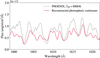 |
Fig. 5 Comparison between the PHOENIX model and the observed photospheric spectrum of β Pic (also shown in Fig. 2), reconstructed from archival observations. Fluxes are provided as observed from Earth (19.3 pc). The spectral region displayed includes several strong Fe II transitions at 1608, 1612, and 1618 Å. |
4.3 Atomic data
In order to compute the statistical equilibrium of each studied species, extensive datasets of transition probabilities, line wavelengths, and effective collision strengths were collected. In most cases, the transition probabilities and line wavelengths were obtained from the National Institute of Standards and Technology (NIST, Kramida et al. 2023) database, and the effective collision strength from CHIANTI (Dere et al. 1997). However, for species with complex spectra, such as Fe II and Ni II, the NIST and CHIANTI datasets were completed with more exhaustive studies (see Table A.1). The hyperfine structure of Mn II (which has a non-zero nuclear spin of I = 5/2) was taken into account, using hyperfine structure constants from Blackwell-Whitehead et al. (2005).
4.4 Interstellar medium
In spectral lines from the ground states of singly ionised species, the signature of LVC #1 overlaps with that of the interstellar medium (ISM). Following Wilson et al. (2017) and Wilson et al. (2019), we modelled the ISM using a temperature of 7000 K, a turbulent broadening parameter of 1.5 km/s, and a RV of −10 km/s in β Pic rest frame. The column density of Fe II in the ISM was measured to be 1.3 ± 0.1 × 1013 cm−2 using the HST spectrum obtained on December 6, 1997, which do not show any exocomet absorption at velocities below −5 km/s. The ISM column densities of other species were obtained by scaling the column density of Fe II with the gas-phase element fractions of Jenkins (2009), and assuming a depletion strength factor F⋆ = 0 in the Local Bubble. All the gas from the ISM is assumed to be in the ground state.
4.5 Line spread functions
Once calculated, the flux transmitted by the three LVCs, the circumstellar disc and the ISM needs to be convolved with the instrumental line spread function (LSF). The LSF of STIS and COS were retrieved from the Space Telescope Science Institute website1. For STIS, tabulated LSFs are available for only a limited number of apertures; in particular, no LSF is provided for the 31×0.05 NDA aperture. In this case, we adopted the LSF of the 0.1×0.2 aperture, which has a similar width and therefore provides the closest available approximation to the 31×0.05NDA aperture. This choice has no significant impact on our fits, as the studied absorption features are broader than the instrumental LSF. For the HARPS spectrum, we used the LSF calculated by Brandeker (2011) using a two-Gaussian profile.
4.6 Fit to the data
Each of the 4 studied components (the three LVCs and the disc) is described by 13 parameters: the 7 column densities of the studied species, and the 6 physical parameters presented in Sect. 3 (the distance to the star, d; the central velocity, v, and Doppler parameter, b; the electronic density, ne, and temperature, Te; and the ratio between the transverse and radial column densities of the cloud, f). In total, the 4 components are thus described by 52 parameters. However, the RV of the disc was fixed to 0 km/s in β Pic rest frame, resulting in 51 free parameters.
Our model was fitted to all the optically allowed transitions arising from the main stable and metastable states of the studied species (340 transitions per component, yielding a total of 1360 absorption lines). Each line was fitted over the full RV range from −15 to +15 km s−1, resulting in a total of 10, 100 degrees of freedom. Most of the studied transitions show clear signatures from the LVCs and the disc, although several non-detected lines were also included in the fit to better constrain some parameters. The fit was performed using a Markov chain Monte Carlo algorithm from the emcee Python package (Foreman-Mackey et al. 2013). 150 independent chains were launched over 30 000 steps, discarding the first 20 000 steps as burn-in.
4.7 Wavelength shifts
Our initial fit matched the observed spectrum reasonably well, yielding a reduced χ2 of 1.78. This value, however, exceeds unity, indicating that the observed data are not fully reproduced.
An important source of discrepancy appeared to rise from the imperfect wavelength calibration of the STIS data. Many lines are indeed detected at a slightly lower or higher wavelength than expected from NIST, with typical shifts of 0.5–1 km/s. This bias is instrumental, as lines covered by several spectral orders often exhibit different shifts from one order to another (see Fig. 6). To correct for this, we applied small RV adjustments to the spectral regions were wavelength offsets were noted. These corrections were restricted to the strongest lines, for which the RV shift could be reliably identified and measured (through a χ2 minimisation). This allowed us to significantly improve the fit, reaching a reduced χ2 of 1.51.
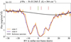 |
Fig. 6 View of the Fe II line at 2365 Å, covered by two orders of the same STIS spectrum. A clear wavelength offset is visible between the two orders; here order #5 is found to be redshifted by 0.5 km/s compared to order #6. The red and green ticks respectively mark the RV of the three LVCs and the disc. |
4.8 Systematic uncertainties
The value of the final reduced χ2 (1.51) remains well above unity. The remaining mismatch between our model and the observed spectrum can be explained by several factors:
First, our model is highly simplified. In reality, exocometary tails likely have complex geometries, non-Gaussian line-profiles, and non-homogeneous temperature and density profiles, resulting in a much more complicated absorption spectrum than produced by our model.
Our transmission model also relies on extensive datasets of oscillator strengths and effective collisions strengths, which are generally accurate within 10%, at best. For instance, most Fe II and Ni II lines listed in NIST are classified as B or B+, corresponding to uncertainties of 10 and 7% on the transition probabilities, respectively. Similarly, effective collision strengths for Fe II, taken from Tayal & Zatsarinny (2018), are accurate to within about 10% for the ground multiplets.
Finally, only four transiting components are modelled (the three LVCs and the disc). In practice, however, the star could be occulted by additional, minor components, not clearly detected in optically thin lines but affecting our fit in the strongest lines.
These sources of uncertainties are difficult to model directly. To account for them, we introduced, for each pixel k, a systematic error σk, sys, to be added quadratically to the tabulated noise. We assumed that, once the data are normalised by the reference spectrum, the systematic uncertainty depends mainly on the absorption depth. To quantify this dependence, the fitted pixels were grouped into categories according to their absorption depths: 0–5%, 5–10%, 10–15%, and so on, up to 95–100%. For each category, we determined the systematic error σsys that, when added in quadrature to the tabulated noise, brings the reduced χ2 of the corresponding pixels to unity. The result of this calculation is shown on Fig. 7: the systematic uncertainty reaches ~4% of the continuum for pixels at ~50% absorption depth (which is about 1–2 times larger than the tabulated noise), and ~1% when the absorption depth is close to 0 or 1. The systematic errors shown on Fig. 7 were then fitted with a fourth-order polynomial, which allowed us to compute the systematic error σk, sys of any pixel k, based on its absorption depth. The χ2 of our model was then computed as
![Mathematical equation: $\[\chi^2=\sum_k \frac{\left(f_{k, ~\mathrm{obs}}-f_{k, ~\mathrm{model}}\right)^2}{\sigma_{k, ~\mathrm{tab}}^2+\sigma_{k, ~\mathrm{sys}}^2},\]$](/articles/aa/full_html/2026/03/aa57819-25/aa57819-25-eq19.png)
where fk, obs, fk, model and σk, tab are respectively the observed flux, the modelled flux, and the instrument pipeline tabulated uncertainties, normalised by the reference spectrum.
It should be noted that this method does not account for possible correlations between the systematic uncertainties of adjacent pixels. Nevertheless, it allows us to obtain more realistic estimates of the uncertainties on the fitted parameters. Running again the fit with the systematic uncertainties included yielded a reduced χ2 of 0.97, close to unity. The mean value and error bars of the fitted parameters were then estimated from the posterior distribution of the Markov chains, and are provided in Table B.1.
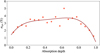 |
Fig. 7 Estimation of the systematic uncertainty of our model (expressed in percentage of the reference spectrum). Dots show the measured systematic uncertainties (σsys) for pixels grouped by absorption depth. The solid line is a fit with a fourth-order polynomial, used to estimate the systematic uncertainty (σk, sys) of each pixel based on its absorption depth. |
5 Overview of the fitted model
Our best-fit model is shown in Fig. 8 around several Fe II, Ni II, and Si II lines (among a total of 340 lines), together with the observed spectrum. Additional examples covering lines from all the studied species are provided in Appendix C.
Despite the limitations detailed above (Sect. 4.8), our model fits remarkably well the observed spectrum. The absorption signatures of the three LVCs and the circumstellar disc are well reproduced across all the studied species, all excitation levels, and over a large range of oscillator strengths, with no exceptions (see e.g. Fig. 8). In particular, the excitation state of Fe II is well captured, up to very high excitation energies (El ~ 30 000 cm−1). This allows us to place tights constraints on the transit distance of each component (Sect. 5.1) and on their compositions (Sect. 6.2). Besides Fe II, the model also reproduces the complex excitation states of Ni II and Cr II in both the LVCs and the disc, further confirming the robustness of our model.
5.1 Transit distances and excitations states
As anticipated in Sect. 2.3, our model places the three LVCs at significantly different distances from the star: 0.88 ± 0.08 au for LVC #1, 4.7 ± 0.3 au for LVC #2, and 1.52 ± 0.15 au for LVC #3. These distances are primarily constrained by the many Fe II lines detected in our spectrum, which arise from a wide range of stable and metastable states with energy between 0 and 30 000 cm−1. As pointed out in Vrignaud & Lecavelier des Etangs (2024), the relative population of these levels is determined by the amount of UV radiation reaching the gas, and thus by the distance to the star. Very close to β Pic, exchanges between excitation states are dominated by the absorption and emission of UV photons, driving the excitation temperature towards ~8000 K (the effective temperature of β Pic). Conversely, at large distances from the star, UV pumping becomes negligible and metastable levels decay towards the ground state via forbidden infrared transitions. The three LVCs studied here are in a intermediate regime, where the excitation state is set by the balance between between UV radiative pumping and the radiative decay of metastable states.
Figure 9 provides the excitation diagrams of Fe II in the three LVCs for the most easily detected states. Crosses show the level populations calculated using our best-fit model, while dots with error bars show direct measurements of the level populations in the LVCs. These estimates were obtained by varying the column density NFe II, i of each excitation state i individually, keeping all other levels fixed, and finding the value that best reproduces the data. The modelled and measured excitation diagrams agree very well for all three LVCs, with most level populations being accurately predicted to within 10%. Owing to its larger distance to β Pic, LVC #2 is, by far, the least excited component: all metastable states above 2400 cm−1 are depleted by 0.3 to 1 dex compared to the two others LVCs, while the ground state is enhanced by 0.3 dex. In addition, we note that the three LVCs exhibit smaller populations of very excited Fe II states (≥30 000 K) compared to the exocomet observed on December 6, 1997, and analysed in Vrignaud & Lecavelier des Etangs (2024), which was found to transit at less than 0.4 au. This illustrates the tight dependence between the transit distance of an exocometary tail and the excitation state of the gas.
In addition to Fe II, the two species that provide the strongest constraints on the transit distance are Cr II and Ni II, as they are detected in multiple electronic configurations. To verify that Fe II, Ni II, and Cr II yield consistent estimates of d, we performed three additional fits in which the lines of each species were fitted independently. We find that these fits constrain the transit distances of the LVCs to similar values (Fig. 10), demonstrating the robustness of our transit distance estimates.
Our fit places the circumstellar disc at ![Mathematical equation: $\[38_{-11}^{+15}\]$](/articles/aa/full_html/2026/03/aa57819-25/aa57819-25-eq20.png) au from β Pic. Unlike the three LVCs, this distance is primarily constrained by the abundance of the Ni II level at 8393 cm−1, which remains substantially populated even at large distance from β Pic. In practice, the inferred distance corresponds to the average radius of the ionised disc, which has a significant radial extent (e.g. Brandeker et al. 2004). Probing this radial extent with the method developed here is, however, difficult, because absorption spectroscopy only provides access to the global level populations in the disc, integrated along the line of sight. Allowing the disc to have a non-zero radial extent does not improve the fit; for instance, placing the disc at a single distance of ~40 au, ordistributing it uniformly from 20 to 60 au, provide fits that are equally good.
au from β Pic. Unlike the three LVCs, this distance is primarily constrained by the abundance of the Ni II level at 8393 cm−1, which remains substantially populated even at large distance from β Pic. In practice, the inferred distance corresponds to the average radius of the ionised disc, which has a significant radial extent (e.g. Brandeker et al. 2004). Probing this radial extent with the method developed here is, however, difficult, because absorption spectroscopy only provides access to the global level populations in the disc, integrated along the line of sight. Allowing the disc to have a non-zero radial extent does not improve the fit; for instance, placing the disc at a single distance of ~40 au, ordistributing it uniformly from 20 to 60 au, provide fits that are equally good.
The typical radius of the disc is comparable, yet smaller, than values obtained from ground-based imagery in Fe I, Na I and Ca II (Olofsson et al. 2001; Brandeker et al. 2004; Nilsson et al. 2012), which generally find the gas distribution to peak around 100 au. This difference could be due to the difference of spatial distribution between neutral and ionised species, as Fe I and Na I are quickly photo-ionised close to β Pic. In addition, the inner disc is difficult to probe in direct imaging due to its high opacity.
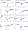 |
Fig. 8 Comparison between the observed spectrum and the fitted model for Fe II, Ni II, and Si II lines. The observed spectrum is shown with a blue line; errors bars reflect the uncertainties tabulated by the STIS pipeline (see Sect. 4.8). The solid orange line shows the reference spectrum. Absorptions from the LVCs, the disc, and the ISM are shown in dashed, solid, and dotted grey lines, respectively. The full model, convolved by the STIS LSF, is shown as a solid black line. Red ticks indicate the central velocities of the three LVCs, while the green tick at 0 km/s indicates the RV of the disc. |
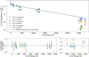 |
Fig. 9 Excitation Fe II in the three LVCs. Top: comparison of the excitation diagram of Fe II measured in the three LVCs (dots with error bars) with the result from our excitation model (crosses). For clarity, we only show levels with significant detections. The solid black line indicates the excitation temperature measured by Vrignaud & Lecavelier des Etangs (2024) in a β Pic exocomet observed on December 6, 1997, and located <0.4 au from the star. By comparison, LVCs #1 and #3 (blue and orange dots) are at located at ~1 au; and LVCs #2 (green dots) is much farther away (4.7 au). Bottom: ratio of the measured and modelled abundances of the studied Fe II levels. The horizontal dotted line indicates the ratio of 1. |
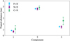 |
Fig. 10 Transit distances of the three LVCs derived from independent fits to the Fe II, Ni II, and Cr II lines. The three species provide similar constraints on the transit distances of the LVCs. |
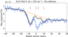 |
Fig. 11 Plot of our model in the 1816 Å Si II line in the case where electronic collisions are disabled. The fit is poor, particularly for LVC #2 and for the disc, because far from β Pic, UV pumping is inefficient at populating the excited Si II level at 287 cm−1. Collisions must be taken into account in the model to properly fit the data (see the bottom panel of Fig. 8). |
5.2 The transverse size
The parameter f, which characterises the ratio between the radial and transverse column densities of each component, is constrained to values between 0.09 and 0.20 for the three LVCs. These values suggest that the LVCs are about 5 times more extended in the radial direction than in the transverse direction. The f parameter of the disc is not constrained by our fit.
The inferred distances of the three LVCs are not very sensitive to f: repeating the fit while imposing f = 0 for all components yields similar distance estimates (within 10%). However, introducing the parameter f significantly improves the fit quality, with a reduced χ2 of 9800 compared to 11 000 when f = 0.
5.3 Temperatures and electronic densities
The excitation states of the studied species are primarily set by radiative excitation, in all four components. As a result, probing the electronic density and temperature is difficult. For LVC #1 and #3, we only obtain upper limits on ne, respectively <106 and <105 cm−3. For these components, including collisions does not significantly improve the fit. For LVC #2, we find that collisions do improve the fit, particularly in Si II and Fe II lines (see Fig. 11). This is because LVC #2 is located further out, and has a stronger self-opacity, leading to weaker radiative excitation. For this component, we constrain log(ne [cm−3]) = 3.3 ± 0.3 and log (Te [K]) = 2.9 ± 0.3. Finally, for the disc, we obtain log (ne [cm−3]) = 2.7 ± 0.3 and log (Te [K]) = 2.9 ± 0.3. These estimates are broadly consistent with the recent results of Wu et al. (2025), which conducted a detailed modelling of the photochemistry along the β Pic disc and found that the electronic density and temperature decrease from ~104 cm−3 and 103 K at 10 au, to 10 cm−3 and 50 K at 200 au.
6 Discussion
6.1 Large transit distances
The transit distances of the three LVCs (0.88, 4.7 and 1.52 au) are much larger than the typical values obtained for high-velocity exocomets using acceleration measurements (0.02–0.14 au; Kennedy 2018). This is not contradictory, however, as all the exocomets analysed by Kennedy (2018) belong to the S family, located closer to β Pic than the D family (to which the LVCs belong). The absorption signatures of the three LVCs in Ca II do not show any acceleration or temporal variation over the 2.25 hours of HARPS monitoring, supporting the fact that they are located far from the star. In addition, around β Pic, the maximum RV for a bound object transiting at 1 au is ~55 km s−1 (25 km s−1 at 5 au). The low RVs of the three LVCs (−7.5, +2.5 and 10 km/s) are thus consistent with objects transiting at 1–5 au and having either small periastron longitudes or small eccentricities and periastron distances similar to the measured transit distances.
Nonetheless, the transit distances of the three LVCs contradict the results of Kiefer et al. (2014b), who inferred a typical transit distance of 19 ± 4 R⋆ for the D family. Their estimates, based on converting the projected size of an exocomet into its distance to β Pic using the hydrodynamical model of Beust & Tagger (1993), are however subject to important limitations. Several assumptions from the model of Beust & Tagger (1993) now appear to be unrealistic, particularly that the ion dynamics can be treated using collisions with a neutral hydrogen cloud. Recent studies (Vrignaud et al. 2024, 2025) have shown that the tails of β Pic exocomets are mostly ionised, and that drag forces are dominated by Coulombian interactions between ions. This completely modifies the global dynamics of the tail, and therefore the link between the distance of a comet from β Pic and the shape of its absorption profile.
Finally, the transit distances of the three LVCs (0.88, 4.7 and 1.52 au) are surprisingly high as, at 1 au or more, the sublimation of refractory dust is very slow, if not impossible. Depending on the dust size and composition, the sublimation lines of silicates around β Pic lie between 0.1 and 0.5 au (Beust et al. 1996, 1998, 2001). At larger distances, exocomets should not release significant amounts of refractory ions. Yet, this is not what is observed: the amount of Si II found in LVC#2 (~5 × 1014 cm−2 covering the full stellar disc) corresponds to the full sublimation of ~1 km3 of SiO2, assuming a density of 2.3 g/cm3. Such large quantities of Si II ions can only be produced by the complete sublimation of dense dust tails, if not whole cometary nuclei, at very short distance to the star. Thus, it seems that the large amounts of refractory ions found in the three LVCs were originally produced close to β Pic (<0.5 au), and subsequently transported to more distant regions. The mechanisms driving this migration are unclear; no study of the long-term evolution of cometary tails in the β Pic system is available. In the models of Beust et al. (1990) and Beust & Tagger (1993), refractory ions (Ca II, Mg II, Al III, etc) are assumed to evolve in a surrounding cloud of neutral hydrogen; as a result, they are not efficiently retained and rapidly escape the tail due to radiation pressure. However, if the cometary tails are ionised (which appears to be the case; Vrignaud et al. 2025), the gas may remain well mixed for a much longer time, allowing it to expand and reach large stellocentric distances without being disrupted. Further modelling of the dynamics of exocometary tails in the β Pic system are in preparation to better understand this behaviour, and in particular to explain why the studied LVCs are not observed to be strongly blueshifted despite having migrated outwards by one or several au.
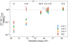 |
Fig. 12 Abundance of the studied species relative to Fe II and normalised by the solar abundance ratios of the corresponding elements, plotted as a function of the ionisation potential. |
6.2 Ionisation state of the gas
The relative abundances of the various studied species in the three LVCs and in the disc are provided in Table B.2. The composition of the four components is also illustrated by Fig. 12, where the abundance ratios (e.g. Ca II/Fe II) are re-normalised by the solar ratios of the corresponding elements (e.g. Ca/Fe).
A clear dichotomy appears between species with ionisation energy in the 15–18 eV range (e.g. Mn II, Fe II, and Ni II), whose abundances are quasi-solar both in the disc and in the LVCs, and species with lower ionisation potentials (S I and Ca II; 10–12 eV), which are more depleted. This behaviour was already identified in Vrignaud et al. (2025) for exocomets at higher redshifts. In addition, easily ionised species appear to be more abundant in the disc and LVC #2 than in LVCs #1 and #3, located closer to β Pic. The Ca II/Fe II ratio of the disc is consistent with solar abundances, while it is 0.2× solar in LVC#2, and 0.08× solar in LVCs #1 and 3. Similarly, we find a S I/Fe II ratio 0.1× solar in the disc, 0.04× solar in LVC #2, and only 0.02× solar in LVCs #1 and #3. The transiting components thus appear to have different ionisation states, in strong correlation with their transiting distances: components located further out in the system are also less ionised. In particular, Ca seems to be mostly present as Ca II in the disc, while in the LVCs it is mostly ionised into Ca III (as shown by the low Ca II/Fe II ratio). Interestingly, the Ca II/Fe II ratios of LVCs #1 and #3 are very similar to the Ca II/Fe II measured in Vrignaud et al. (2025) for exocomets at shorter distances and larger velocities (Ca II/Fe II = 0.082 ± 0.019 × solar), indicating that their ionisation state is somehow similar to that of HVCs.
7 Conclusion
We have presented a new approach to measuring the transit distance of exocometary tails based on the excitation state of the gas. This method relies on the fact that, in diluted gaseous tails, the excitation state is primarily set by the absorption of photons coming from the star. The relative population of excited levels then only depends on the intensity of the incoming radiation and, therefore, on the distance to the star.
We applied this approach to three low-velocity exocomets in the β Pic system observed on April 29, 2025, with the HST and HARPS. We developed a detailed model of the absorption spectrum of these comets, where the excitation and the transmitted flux are computed iteratively along the line of sight within each gaseous cloud. Our model was fitted to the observations, allowing us to recover the transit distance and composition of the three exocomets.
The measured transit distances of the three studied exocomets (0.88 ± 0.08, 4.7 ± 0.3, and 1.52 ± 0.15 au) are much larger than previous estimates for low-velocity objects in the β Pic system (19 ± 4 R⋆ = 0.14 ± 0.03 au; Kiefer et al. 2014b). These distances are also surprising as, at 1 au or more from β Pic, dust sublimation is very inefficient, which is in contradiction with the large amounts of refractory ions found in the exocometary tails. This suggests that exocomet gaseous tails in the β Pic system, most likely produced very close to the star (<0.5 au), can migrate over large distances without being disrupted, and remain detectable even several au from β Pic.
Acknowledgements
We thank the anonymous reviewer for their careful reading of this paper and for their constructive feedback. We gratefully acknowledge funding from the Centre National d’Etudes Spatiales (CNES).
References
- Apai, D., Schneider, G., Grady, C. A., et al. 2015, ApJ, 800, 136 [NASA ADS] [CrossRef] [Google Scholar]
- Asplund, M., Amarsi, A. M., & Grevesse, N. 2021, A&A, 653, A141 [NASA ADS] [CrossRef] [EDP Sciences] [Google Scholar]
- Beust, H., & Tagger, M. 1993, Icarus, 106, 42 [NASA ADS] [CrossRef] [Google Scholar]
- Beust, H., Lagrange-Henri, A. M., Vidal-Madjar, A., & Ferlet, R. 1989, A&A, 223, 304 [NASA ADS] [Google Scholar]
- Beust, H., Lagrange-Henri, A. M., Vidal-Madjar, A., & Ferlet, R. 1990, A&A, 236, 202 [NASA ADS] [Google Scholar]
- Beust, H., Lagrange, A. M., Plazy, F., & Mouillet, D. 1996, A&A, 310, 181 [NASA ADS] [Google Scholar]
- Beust, H., Lagrange, A. M., Crawford, I. A., et al. 1998, A&A, 338, 1015 [NASA ADS] [Google Scholar]
- Beust, H., Karmann, C., & Lagrange, A. M. 2001, A&A, 366, 945 [NASA ADS] [CrossRef] [EDP Sciences] [Google Scholar]
- Beust, H., Milli, J., Morbidelli, A., et al. 2024, A&A, 683, A89 [NASA ADS] [CrossRef] [EDP Sciences] [Google Scholar]
- Blackwell-Whitehead, R. J., Toner, A., Hibbert, A., Webb, J., & Ivarsson, S. 2005, MNRAS, 364, 705 [NASA ADS] [CrossRef] [Google Scholar]
- Brandeker, A. 2011, ApJ, 729, 122 [NASA ADS] [CrossRef] [Google Scholar]
- Brandeker, A., Liseau, R., Olofsson, G., & Fridlund, M. 2004, A&A, 413, 681 [NASA ADS] [CrossRef] [EDP Sciences] [Google Scholar]
- Brandeker, A., Cataldi, G., Olofsson, G., et al. 2016, A&A, 591, A27 [NASA ADS] [CrossRef] [EDP Sciences] [Google Scholar]
- Cassidy, C. M., Hibbert, A., & Ramsbottom, C. A. 2016, A&A, 587, A107 [NASA ADS] [CrossRef] [EDP Sciences] [Google Scholar]
- Chen, C. H., Lu, C. X., Worthen, K., et al. 2024, ApJ, 973, 139 [Google Scholar]
- Crifo, F., Vidal-Madjar, A., Lallement, R., Ferlet, R., & Gerbaldi, M. 1997, A&A, 320, L29 [NASA ADS] [Google Scholar]
- Dent, W. R. F., Wyatt, M. C., Roberge, A., et al. 2014, Science, 343, 1490 [NASA ADS] [CrossRef] [Google Scholar]
- Dere, K. P., Landi, E., Mason, H. E., Monsignori Fossi, B. C., & Young, P. R. 1997, A&AS, 125, 149 [NASA ADS] [CrossRef] [EDP Sciences] [Google Scholar]
- Ferlet, R., Hobbs, L. M., & Vidal-Madjar, A. 1987, A&A, 185, 267 [NASA ADS] [Google Scholar]
- Foreman-Mackey, D., Hogg, D. W., Lang, D., & Goodman, J. 2013, PASP, 125, 306 [Google Scholar]
- Heap, S. R., Lindler, D. J., Lanz, T. M., et al. 2000, ApJ, 539, 435 [Google Scholar]
- Hoeijmakers, H. J., Jaworska, K. P., & Prinoth, B. 2025, A&A, 700, A239 [NASA ADS] [CrossRef] [EDP Sciences] [Google Scholar]
- Husser, T. O., Wende-von Berg, S., Dreizler, S., et al. 2013, A&A, 553, A6 [NASA ADS] [CrossRef] [EDP Sciences] [Google Scholar]
- Jenkins, E. B. 2009, ApJ, 700, 1299 [Google Scholar]
- Kennedy, G. M. 2018, MNRAS, 479, 1997 [NASA ADS] [CrossRef] [Google Scholar]
- Kiefer, F., Lecavelier des Etangs, A., Augereau, J. C., et al. 2014a, A&A, 561, L10 [NASA ADS] [CrossRef] [EDP Sciences] [Google Scholar]
- Kiefer, F., Lecavelier des Etangs, A., Boissier, J., et al. 2014b, Nature, 514, 462 [Google Scholar]
- Kramida, A., Yu. Ralchenko, Reader, J., & NIST ASD Team. 2023, NIST Atomic Spectra Database (ver. 5.11), [Online]. Available: https://physics.nist.gov/asd [2023, December 15]. National Institute of Standards and Technology, Gaithersburg, MD [Google Scholar]
- Lagrange, A. M., Vidal-Madjar, A., Deleuil, M., et al. 1995, A&A, 296, 499 [NASA ADS] [Google Scholar]
- Lagrange, A. M., Bonnefoy, M., Chauvin, G., et al. 2010, Science, 329, 57 [Google Scholar]
- Lagrange, A. M., Meunier, N., Rubini, P., et al. 2019, Nat. Astron., 3, 1135 [NASA ADS] [CrossRef] [Google Scholar]
- Lecavelier des Etangs, A., Perrin, G., Ferlet, R., et al. 1993, A&A, 274, 877 [NASA ADS] [Google Scholar]
- Lecavelier des Etangs, A., Cros, L., Hébrard, G., et al. 2022, Sci. Rep., 12, 5855 [NASA ADS] [CrossRef] [Google Scholar]
- Lecavelier des Etangs, A., Strøm, P. A., & Seligman, D. Z. 2026, Space Sci. Rev., 222, 12 [Google Scholar]
- Liggins, F. S., Pickering, J. C., Nave, G., et al. 2021, ApJ, 907, 69 [Google Scholar]
- Meléndez, M., Bautista, M. A., & Badnell, N. R. 2007, A&A, 469, 1203 [Google Scholar]
- Miles, B. E., Roberge, A., & Welsh, B. 2016, ApJ, 824, 126 [NASA ADS] [CrossRef] [Google Scholar]
- Miret-Roig, N., Galli, P. A. B., Brandner, W., et al. 2020, A&A, 642, A179 [NASA ADS] [CrossRef] [EDP Sciences] [Google Scholar]
- Nilsson, H., Ljung, G., Lundberg, H., & Nielsen, K. E. 2006, A&A, 445, 1165 [NASA ADS] [CrossRef] [EDP Sciences] [Google Scholar]
- Nilsson, R., Brandeker, A., Olofsson, G., et al. 2012, A&A, 544, A134 [NASA ADS] [CrossRef] [EDP Sciences] [Google Scholar]
- Nowak, M., Lacour, S., Lagrange, A. M., et al. 2020, A&A, 642, L2 [NASA ADS] [CrossRef] [EDP Sciences] [Google Scholar]
- Okamoto, Y. K., Kataza, H., Honda, M., et al. 2004, Nature, 431, 660 [CrossRef] [Google Scholar]
- Olofsson, G., Liseau, R., & Brandeker, A. 2001, ApJ, 563, L77 [Google Scholar]
- Pavlenko, Y., Kulyk, I., Shubina, O., et al. 2022, A&A, 660, A49 [NASA ADS] [CrossRef] [EDP Sciences] [Google Scholar]
- Rebollido, I., Stark, C. C., Kammerer, J., et al. 2024, AJ, 167, 69 [NASA ADS] [CrossRef] [Google Scholar]
- Roberge, A., Feldman, P. D., Lagrange, A. M., et al. 2000, ApJ, 538, 904 [NASA ADS] [CrossRef] [Google Scholar]
- Smith, B. A., & Terrile, R. J. 1984, Science, 226, 1421 [Google Scholar]
- Storey, P. J., Zeippen, C. J., & Sochi, T. 2016, MNRAS, 456, 1974 [CrossRef] [Google Scholar]
- Tayal, S. S., & Zatsarinny, O. 2018, Phys. Rev. A, 98, 012706 [NASA ADS] [CrossRef] [Google Scholar]
- Tayal, S. S., & Zatsarinny, O. 2020, ApJ, 888, 10 [Google Scholar]
- Tobin, W., Barnes, S. I., Persson, S., & Pollard, K. R. 2019, MNRAS, 489, 574 [NASA ADS] [CrossRef] [Google Scholar]
- Vidal-Madjar, A., Lagrange-Henri, A. M., Feldman, P. D., et al. 1994, A&A, 290, 245 [NASA ADS] [Google Scholar]
- Vrignaud, T., & Lecavelier des Etangs, A. 2024, A&A, 691, A2 [NASA ADS] [CrossRef] [EDP Sciences] [Google Scholar]
- Vrignaud, T., Lecavelier des Etangs, A., Kiefer, F., et al. 2024, A&A, 684, A210 [NASA ADS] [CrossRef] [EDP Sciences] [Google Scholar]
- Vrignaud, T., Lecavelier des Etangs, A., Strøm, P. A., & Kiefer, F. 2025, A&A, 697, A21 [NASA ADS] [CrossRef] [EDP Sciences] [Google Scholar]
- Wilson, P. A., Lecavelier des Etangs, A., Vidal-Madjar, A., et al. 2017, A&A, 599, A75 [NASA ADS] [CrossRef] [EDP Sciences] [Google Scholar]
- Wilson, P. A., Kerr, R., Lecavelier des Etangs, A., et al. 2019, A&A, 621, A121 [NASA ADS] [CrossRef] [EDP Sciences] [Google Scholar]
- Wu, Y., Worthen, K., Brandeker, A., & Chen, C. 2025, ApJ, 982, 123 [Google Scholar]
- Zieba, S., Zwintz, K., Kenworthy, M. A., & Kennedy, G. M. 2019, A&A, 625, L13 [NASA ADS] [CrossRef] [EDP Sciences] [Google Scholar]
See the tabulated LSFs for STIS an COS on www.stsci.edu/hst/instrumentation/
Appendix A Fitted species
Species included in the model.
Appendix B Fitted parameters and compositions
Parameters fitted by the model.
Abundances in the three LVCs and the circumstellar disc, normalised to Fe II.
Appendix C Examples of lines in the April 29, 2025, spectrum
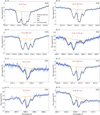 |
Fig. C.1 Examples of lines studied in the present paper. The reference spectrum is indicated with a solid orange line. Absorptions from the ISM, from the three LVCs, and from the circumstellar disc are shown with dotted, dashed, and solid grey lines, respectively. The full model, convolved with the instrumental LSF, is shown with a solid black line. The observed spectrum is shown in blue; error bars only reflect the tabulated uncertainties and do not include the systematic uncertainties of our model (Sect. 4.8). For each line, the corresponding species and lower level energy are indicated in red. Note that the Fe II line profile at 2494 Å results from a doublet of two lines separated by about 0.1 Å. |
All Tables
All Figures
|
Fig. 1 Spectroscopic observations of β Pic obtained on April 29, 2025. The HARPS spectrum is not flux-calibrated and was simply re-normalised to a flux level similar to that of the STIS data. Numerous saturated absorption lines are visible in the STIS and HARPS spectra, attributed to Si II, C I, Al II, Fe II, Mg II, and Ca II. The HST spectra are consistent with a stellar model from the PHOENIX library (thick grey line; Husser et al. 2013) at Teff = 8000 K (see Sect. 4.1). |
| In the text | |
|
Fig. 2 Zoomed-in view of the STIS spectra of β Pic from April 29, 2025, around two Fe II lines. Top: view of the strong Fe II line at 2756.5 Å. Archival STIS spectra of β Pic covering the same line are shown in transparent font. The solid black line represents an estimate of the stellar photospheric continuum, free of circumstellar absorption. Bottom: same view of the shallower Fe II line at 2578.7 Å. This wavelength region is covered by two orders of the STIS echelle spectrograph. Since these two lines arise from excited states of Fe+, they do not show any signature of the circumstellar disc (see Sect. 2.3). |
| In the text | |
|
Fig. 3 Zoomed-in view of the STIS spectra of β Pic obtained on April 29, 2025, around four Fe II lines arising from different excitation levels. Errors bars were tabulated from the STIS data reduction pipeline. Red ticks indicate the velocities of the three main LVCs. The circumstellar disc (green tick, 0 km/s) is detected in the ground state of Fe II. Note that the λλ2260 and 2622 Å lines are covered by two spectral orders. |
| In the text | |
|
Fig. 4 Same as Fig. 3 but for two Ni II lines and two Si II lines. The disc is detected in the metastable state of Ni II at 8393 cm−1, and in the ground state of Si II. |
| In the text | |
|
Fig. 5 Comparison between the PHOENIX model and the observed photospheric spectrum of β Pic (also shown in Fig. 2), reconstructed from archival observations. Fluxes are provided as observed from Earth (19.3 pc). The spectral region displayed includes several strong Fe II transitions at 1608, 1612, and 1618 Å. |
| In the text | |
|
Fig. 6 View of the Fe II line at 2365 Å, covered by two orders of the same STIS spectrum. A clear wavelength offset is visible between the two orders; here order #5 is found to be redshifted by 0.5 km/s compared to order #6. The red and green ticks respectively mark the RV of the three LVCs and the disc. |
| In the text | |
|
Fig. 7 Estimation of the systematic uncertainty of our model (expressed in percentage of the reference spectrum). Dots show the measured systematic uncertainties (σsys) for pixels grouped by absorption depth. The solid line is a fit with a fourth-order polynomial, used to estimate the systematic uncertainty (σk, sys) of each pixel based on its absorption depth. |
| In the text | |
|
Fig. 8 Comparison between the observed spectrum and the fitted model for Fe II, Ni II, and Si II lines. The observed spectrum is shown with a blue line; errors bars reflect the uncertainties tabulated by the STIS pipeline (see Sect. 4.8). The solid orange line shows the reference spectrum. Absorptions from the LVCs, the disc, and the ISM are shown in dashed, solid, and dotted grey lines, respectively. The full model, convolved by the STIS LSF, is shown as a solid black line. Red ticks indicate the central velocities of the three LVCs, while the green tick at 0 km/s indicates the RV of the disc. |
| In the text | |
|
Fig. 9 Excitation Fe II in the three LVCs. Top: comparison of the excitation diagram of Fe II measured in the three LVCs (dots with error bars) with the result from our excitation model (crosses). For clarity, we only show levels with significant detections. The solid black line indicates the excitation temperature measured by Vrignaud & Lecavelier des Etangs (2024) in a β Pic exocomet observed on December 6, 1997, and located <0.4 au from the star. By comparison, LVCs #1 and #3 (blue and orange dots) are at located at ~1 au; and LVCs #2 (green dots) is much farther away (4.7 au). Bottom: ratio of the measured and modelled abundances of the studied Fe II levels. The horizontal dotted line indicates the ratio of 1. |
| In the text | |
|
Fig. 10 Transit distances of the three LVCs derived from independent fits to the Fe II, Ni II, and Cr II lines. The three species provide similar constraints on the transit distances of the LVCs. |
| In the text | |
|
Fig. 11 Plot of our model in the 1816 Å Si II line in the case where electronic collisions are disabled. The fit is poor, particularly for LVC #2 and for the disc, because far from β Pic, UV pumping is inefficient at populating the excited Si II level at 287 cm−1. Collisions must be taken into account in the model to properly fit the data (see the bottom panel of Fig. 8). |
| In the text | |
|
Fig. 12 Abundance of the studied species relative to Fe II and normalised by the solar abundance ratios of the corresponding elements, plotted as a function of the ionisation potential. |
| In the text | |
|
Fig. C.1 Examples of lines studied in the present paper. The reference spectrum is indicated with a solid orange line. Absorptions from the ISM, from the three LVCs, and from the circumstellar disc are shown with dotted, dashed, and solid grey lines, respectively. The full model, convolved with the instrumental LSF, is shown with a solid black line. The observed spectrum is shown in blue; error bars only reflect the tabulated uncertainties and do not include the systematic uncertainties of our model (Sect. 4.8). For each line, the corresponding species and lower level energy are indicated in red. Note that the Fe II line profile at 2494 Å results from a doublet of two lines separated by about 0.1 Å. |
| In the text | |
Current usage metrics show cumulative count of Article Views (full-text article views including HTML views, PDF and ePub downloads, according to the available data) and Abstracts Views on Vision4Press platform.
Data correspond to usage on the plateform after 2015. The current usage metrics is available 48-96 hours after online publication and is updated daily on week days.
Initial download of the metrics may take a while.