| Issue |
A&A
Volume 707, March 2026
|
|
|---|---|---|
| Article Number | A324 | |
| Number of page(s) | 18 | |
| Section | Stellar structure and evolution | |
| DOI | https://doi.org/10.1051/0004-6361/202557860 | |
| Published online | 17 March 2026 | |
Physical properties of long-rising type II supernovae
Bayesian analytic modeling and spectrophotometric correlations
1
Dipartimento di Fisica e Astronomia “Ettore Majorana”, Università degli Studi di Catania, Via Santa Sofia 64, 95123 Catania, Italy
2
INAF – Osservatorio Astrofisico di Catania, Via Santa Sofia 78, 95123 Catania, Italy
3
Cardiff Hub for Astrophysics Research and Technology, School of Physics & Astronomy, Cardiff University, Queens Buildings, The Parade, Cardiff CF24 3AA, UK
4
INFN – Laboratori Nazionali del Sud, Via S. Sofia 62, 95125 Catania, Italy
★ Corresponding author: This email address is being protected from spambots. You need JavaScript enabled to view it.
Received:
27
October
2025
Accepted:
7
February
2026
Abstract
Context. The supernova (SN) 1987A, with its long-rising (≳40 days) light curve, defines a rare subclass of type II SNe known as 1987A-like events. Representing only ∼1–3% of all core-collapse SNe and often found in low-metallicity environments, their large diversity suggests a wide range of progenitor and explosion properties.
Aims. Our aim with this study is to improve the understanding of 1987A-like SNe by characterizing their explosion parameters, including kinetic energy, ejected mass, progenitor radius at the explosion, and synthesized 56Ni mass. Additionally, we seek to identify systematic trends in both the physical properties and the observed spectrophotometric features of these peculiar events.
Methods. A new Bayesian parameter estimation method based on our 56Ni-dependent analytical model for hydrogen-rich SNe is applied to derive explosion parameters from the light curves and expansion velocities of one of the largest and most comprehensive 1987A-like SN samples to date. These data are measured through a consistent analysis of observations available in the literature.
Results. The analysis reveals a heterogeneous population that nevertheless clusters into two main groups: (i) lower-energy explosions with modest 56Ni yields (∼0.07 M⊙), similar to SN 1987A, and (ii) more energetic events (up to ∼5 foe) with larger nickel production and, in some cases, unusually extended progenitors. We confirm a robust correlation between 56Ni mass, peak luminosity, and explosion energy, as well as between ejecta mass and the recombination timescale. An anticorrelation between Ba II line strength and photospheric velocity indicates that stronger Ba II absorptions in 1987A-like SNe arise from more compact, slowly expanding ejecta.
Conclusions. Our findings indicate that 87A-like SNe populate a continuous distribution of explosion energies and progenitor radii. The study underscores the need to extend analytical frameworks to include additional power sources that will enable scalable and accurate modeling of the growing number of peculiar transients that will be discovered by current and upcoming surveys (e.g., ZTF and LSST).
Key words: methods: analytical / methods: data analysis / methods: statistical / supernovae: general / supernovae: individual: 1987A-like SNe
© The Authors 2026
 Open Access article, published by EDP Sciences, under the terms of the Creative Commons Attribution License (https://creativecommons.org/licenses/by/4.0), which permits unrestricted use, distribution, and reproduction in any medium, provided the original work is properly cited.
This article is published in open access under the Subscribe to Open model. This email address is being protected from spambots. You need JavaScript enabled to view it. to support open access publication.
1. Introduction
The explosion of Supernova (SN) 1987A, located only ≈50 kpc from Earth in the direction of the Large Magellanic Cloud (LMC), was an extraordinary event that significantly advanced our understanding of core-collapse (CC) SN events and progenitor stars (e.g., Burrows 1990; Woosley et al. 2002). The unusual shape of its long-rising (≈80 days) light curve (LC) is consistent with the explosion of a compact blue supergiant (BSG) progenitor (Arnett et al. 1989; Kleiser et al. 2011; Orlando et al. 2015). The slow brightness rise and the LC secondary peak, characteristic features of SN 1987A, make it the prototype of a peculiar subclass of H-rich SN events, referred to as long-rising (typically ≳40 days) type II SNe (SNe II), or simply 1987A-like events (e.g., Turatto et al. 2007; Pastorello et al. 2012; Taddia et al. 2016; Pumo et al. 2023, hereafter Paper I).
Notably, 1987A-like SNe are intrinsically rare events, with observational estimates suggesting they account for only ≈1 − 3% of all CC-SNe (Smartt 2009; Pastorello et al. 2012; Taddia et al. 2016; Sit et al. 2023, who recently reported a volumetric rate of about 1.37 × 10⁻⁶ Mpc−3 yr−1). Their rarity reflects the limited evolutionary pathways through which a massive star (with a zero age main sequence mass of MZAMS ≳ 8 − 10 M⊙; e.g., Pumo et al. 2009) can become a BSG prior to its explosion as a CC-SN.
Although the sample of long-rising SNe II is statistically limited, their bolometric LCs exhibit significant variation in rise time (tM) and the maximum luminosity (LM) of the secondary peak (Paper I). This peak, taking place during the hydrogen recombination phase, is commonly interpreted as the result of the interplay between the cooling driven by the SN expansion rate and heating from the radioactive decay of isotopes, primarily 56Ni, synthesized during the explosion (see, e.g., Popov 1993; Utrobin & Chugai 2011; Pumo & Zampieri 2011; Pumo & Cosentino 2025, hereafter Paper II).
Modeling the LC peak and analysing its main features allow us to infer key physical properties of the ejected material (hereafter the ejecta), including the explosion energy (E), progenitor radius (R0), total ejecta mass (Mej), and the mass of radioactive 56Ni (MNi). These quantities, in turn, provide crucial insights into the progenitor’s nature and the explosion mechanism (e.g., Arnett 1996; Kasen & Woosley 2009; Pumo & Zampieri 2013; Fang et al. 2024).
Previous studies about long-rising SNe have identified several clones of SN 1987A (e.g., SN 2009E, SN 2009mw, and SN 2018hna; see also Pastorello et al. 2012; Takáts et al. 2016; Singh et al. 2019), which are characterized by peak luminosities below 2 × 1042 erg s−1 and rise times of approximately 70–90 days. These events are generally interpreted as CC-explosions with energies in the range of ∼0.5 − 5 foe (1 foe ≡ 1051 erg), originating from relatively compact (R0 ∼ 30 − 100 R⊙) and massive (Mej ∼ 15 − 20 M⊙) progenitors (see Paper I, and references therein). The 56Ni masses powering their tail luminosities typically range from MNi ∼ 0.05 − 0.1 M⊙, higher than those of standard type II-plateau (IIP) SNe (see, e.g., Pastorello et al. 2012; Müller et al. 2017; Rodríguez et al. 2021).
There is also evidence that similar long-rising LCs can originate from non-BSG progenitors (R0 ≳ 300 R⊙) capable of synthesizing substantial amounts of 56Ni (MNi ≳ 0.1 M⊙). Examples include SN 2004ek and SN 2004em, which have been described by Taddia et al. (2016) as intermediate events bridging the gap between the clones of SN 1987A and typical SNe IIP. The discovery of brighter 1987A-like objects, including PTF12kso and PTF12gcx (Taddia et al. 2016), seems to indicate the existence of Ni-rich (≳0.1 − 0.2 M⊙) and high-energy (≳5 − 10 foe) events forming a luminous tail of 1987A-like events, which could be characterized by a non-conventional explosion (Paper I). Among these events, OGLE-2014-SN-073 (hereafter OGLE-14) stands out as the brightest long-rising SN (Terreran et al. 2017). With a redshift of z ≃ 0.12, it is also the most distant of 1987A-like SNe, second only to the gravitationally lensed SN Refsdal (z ≃ 1.49, see Kelly et al. 2016). OGLE-14 is characterized by a peak bolometric luminosity of approximately 1043 erg s−1 and a rise time of about 100 days. Its extraordinary LC challenges explanation within the framework of the conventional neutrino-driven CC paradigm and has been linked to pair-instability scenarios (Terreran et al. 2017). An alternative explanation for this exceptional event involves the presence of a prompt injection of energy from a compact internal engine (e.g., magnetar) following the explosion. Such a mechanism has also been proposed for more recent and nearby analogous events, including SN 2020faa (Yang et al. 2021; Salmaso et al. 2023) and SN 2021aatd (Szalai et al. 2024). The influence of additional energy sources, such as 56Ni–56Co decay, magnetar spin-down, or accretion onto a compact object, can extend the long-rising phase and alter the late-time LC (e.g., Kasen & Bildsten 2010; Inserra et al. 2013; Dexter & Kasen 2013; Khatami & Kasen 2019; Matsumoto et al. 2025, and further comments in Paper II). These additional energy sources can give rise to long-lived events such as SN DES16C3cje (Gutiérrez et al. 2020), which exhibited a rise time of approximately 140 days, followed by a decline consistent with fall-back accretion power after 300 days.
Despite their significance, fundamental questions persist regarding 1987A-like SNe, primarily due to the absence of sufficiently accurate and efficient methods for characterizing their physical properties (Paper I; Paper II). Moreover, the available information about the physical properties of the studied sample remains too limited and uncertain to draw definitive conclusions (Paper I). Form 2018 June to 2021 December, the sample of 1987A-like SNe has nearly doubled thanks to the systematic study by Sit et al. (2023) as part of the Census of the Local Universe (CLU; Cook et al. 2019) experiment conducted with the Zwicky Transient Facility (ZTF; Bellm et al. 2018; Graham et al. 2019) on galaxies at less than 200 Mpc (z ≲ 0.05). This study presented the LCs and spectra of 13 additional long-rising SNe. However, a complete physical characterization of their progenitors and explosion mechanisms is still missing.
With the aim of improving our understanding of long-rising type II SN explosions, we present a new Bayesian parameter estimation method based on the LC analytical model developed in Paper II. This approach enables us to infer the physical properties of SN progenitors at the explosion, including E, Mej, R0, and MNi. In this paper, after presenting this method and validating its accuracy (Sect. 2), we apply it to one of the largest and most comprehensive samples of well-observed 1987A-like objects (Sect. 3). Finally, we conduct a global study inside 1987A-like class of their explosion parameters in relation to the measured spectrophotometric features (Sect. 4). The key results are outlined in Section 5, and we highlight their significance in interpreting the nature of these peculiar events.
2. “Fast” SN modeling procedures
The physical characterization of long-rising SNe II can be approached through various modeling methods, each balancing computational complexity and accuracy. The most detailed analyses employ full-numerical hydrodynamic simulations, which incorporate a wide range of physical phenomena, including relativistic hydrodynamics and nuclear heating processes (e.g., Pumo & Zampieri 2011; Bersten et al. 2011). Although the numerical hydrodynamic modeling (HM) is highly accurate, it is computationally expensive and less practical for statistical studies of a heterogeneous sample of peculiar events, such as 1987A-like SNe. A more rapid but less precise alternative is the use of scaling relations, which connect the SN physical parameters to observables through simple proportionality relations. However, the accuracy of this method diminishes when the observed SNe differ significantly from the reference event (e.g., Paper I, and references therein). Intermediate approaches, such as analytical or semi-analytical models, stand out as the most practical solution, as they significantly reduce the complexity of full numerical simulations, minimizing computational time (thus being “faster”) while still capturing the main physical processes involved in the SN post-explosive evolution (see, e.g., Paper II, and references therein).
Among the most well-known and widely used analytic models for H-rich SNe, including 1987A-like events, are those developed by Arnett (1980, 1996) and Arnett et al. (1989), which describe the behavior of the bolometric LC dominated by the diffusion of photons through the expanding SN ejecta. These models are particularly effective during the early post-explosive phases, when hydrogen recombination does not yet significantly influence the cooling emission. For the later stages, when hydrogen recombination becomes important, the standard analytical framework is provided by Popov (1993). Furthermore, this model excludes the presence of additional heating effects, such as those from radioactive decay (e.g., 56Ni–56Co elements), ejecta interactions with the circumstellar medium (CSM), or energy injection from a central compact object. Subsequent analytical approaches have included these additional energy sources retaining the diffusive approximation of Arnett’s models (see, e.g., Chatzopoulos et al. 2012; Inserra et al. 2013; Nicholl et al. 2017; Villar et al. 2017). More recently, similar mechanisms have been analytically incorporated into models for H-rich SNe, allowing for the evaluation of heating source effects on the SN LC even during phases where hydrogen recombination dominates (e.g., Dexter & Kasen 2013; Matsumoto et al. 2025, and Paper II). Specifically, Paper II’s model is the first analytical description to account for different 56Ni distributions and their effect on radioactive heating at the recombination front. These features make it a valuable description for developing new modeling procedures aimed at accurately and efficiently determining the explosion and progenitor parameters of 1987A-like events. In the following, we present our implementation of this framework (Sect. 2.1) and assess its performance by comparing results for a set of well-studied 1987A-like SNe against HM benchmarks (Sect. 2.2).
2.1. Supernova bayesian analytic modeling – SUPERBAM
“Supernova Bayesian Analytic Modeling” (SUPERBAM) is a novel modeling approach based on Bayesian statistics and the analytical model presented in Paper II. It characterizes key physical properties of H-rich SNe, including MNi, E, Mej, and R0, through the analysis of the bolometric LC shape during the recombination phase (e.g., Pumo & Zampieri 2011). To achieve this, SUPERBAM follows a three-phase process:
-
Prior information – SUPERBAM extracts key spectrophotometric features from SN observations to construct prior probability distributions using appropriate scaling equations.
-
Likelihood definition – A likelihood function for the modeling parameters is defined by comparing analytical model predictions with observed data.
-
Posterior exploration – Priors and likelihoods are combined to obtain the posterior distribution, which is then analysed to determine the best-fit SN parameters.
These steps are detailed in the following subsections.
2.1.1. Prior information
SUPERBAM employs physically motivated priors based on empirical scaling relations that link observable quantities, such as LC morphology and photospheric velocity, to the SN explosion parameters. This approach naturally narrows the parameter space without enforcing arbitrary boundaries, thus improving convergence efficiency and reducing the risk of bias near the edges of the physically plausible domain (see, e.g., Silva-Farfán et al. 2024). In contrast to a blind, uniform search over the full multidimensional parameter space (E, Mej, R0, MNi), this method enables a faster and more robust determination of the most probable physical configuration for each SN.
To automatically identify the LC characteristics necessary for defining prior probability, SUPERBAM employs a gaussian process regression1 (GPR), which permits interpolation of the LC, facilitating both its analysis and the computation of its derivative (see, e.g., Fig. 13 in Paper II). To select the best combination of mean function and kernel2 for reproducing light and velocity curves, we tested several configurations using SN 1987A data. In these tests, the curves were artificially down-sampled by randomly removing individual points or entire observing periods of up to 30 days. By comparing the reconstructed values from the GPR against the original data via the mean square deviation, we identified the Matérn 3/2 kernel with a constant mean function as the most effective regression method for this type of data. The Matérn 3/2 kernel models functions with continuous derivatives up to the second order (e.g., Roberts et al. 2013), enabling the reconstruction of smooth profiles even when significant variations in the derivative or changes in concavity are present, as commonly observed in the 1987A-like LCs (see Fig. 1). Since the LC behavior of SN 1987A is representative of the class, the same GPR setup is adopted for all other 1987A-like events.
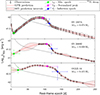 |
Fig. 1. Application of GPR to the bolometric LCs of SN 1987A, SN 2009E, and OGLE-14 taken from the literature (see Ref. in Sect. 2.2) to identify the main LC features. The adopted GPR employs a constant mean function combined with a Matérn 3/2 kernel. For each SN LC, the key epochs tm, |

Once the entire LC is reconstructed through GPR, three characteristic epochs (tm,  , and tf*) are identified to estimate prior constrains. The first one is tm, defined as the epoch of minimum bolometric luminosity after the SN breakout but preceding the maximum of the secondary peak, and it is generally associated with the beginning of the hydrogen recombination (i.e., ti; see also Paper I). The other two epochs,
  and tf*, were already introduced in Paper II and are defined in terms of the bolometric magnitude (i.e., Mbol ≡ −2.5log10Lbol + 88.7). Specifically,
  corresponds to the normalized peak’s maximum where the derivative of Mbol equals to −2.5log10e/(111 day), i.e., the slope of the 56Co decay tail (τ56Co ≃ 111 day; cf. Eq. (22) in Paper II), while tf* is the epoch of maximum derivative, corresponding to the inflection point of Mbol that marks the end of the recombination phase. The uncertainties on these epochs depend both on the GPR reconstruction, strongly linked to the number of observations available in the corresponding LC phase, and on the LC morphology (see Sect. 2.2 for further details). Moreover, the tf* positive error is constrained by the first epoch after the inflection where Ṁbol ≃ −2.5 log10 e/(111 d), which defines the beginning of the radioactive tail.
Considering all observations taken after the upper limit of tf*, the 56Ni mass can be directly estimated by fitting these LC points with the 56Ni–56Co radioactive luminosity, LNi(t) = MNi × ϵ(t), where ϵ(t) is the specific energy release rate (erg g−1 s−1) from the 56Ni → 56Co → 56Fe decay chain (see Eq. (22) in Paper II). In 1987A-like SNe, the trapping of γ-rays from 56Ni–56Co decay remains efficient even beyond 300 − 400 days (see Paper II, and references therein). Since tf* ≫ τ56Ni ≃ 8.8 d, the 56Ni–56Co radioactive luminosity for t > tf* can be expressed as:
 (1)
(1)
Thus, MNi is estimated by performing a linear fit to the logarithm of the bolometric luminosity during the radioactive tail (t > tf*):
![Mathematical equation: $$ \begin{aligned} \log _{10}L_{\rm Bol.}[\mathrm{erg/s}]= 43.18 +\log _{10}M_{\rm Ni}[\mathrm{M}_\odot ]-\frac{t[\mathrm{d}]}{255.6}\cdot \end{aligned} $$](/articles/aa/full_html/2026/03/aa57860-25/aa57860-25-eq6.gif) (2)
(2)
This provides a direct measurement of MNi, one of the four key physical parameters of these SNe, effectively reducing the dimensionality of the inference problem from four free parameters to three.
To constrain the remaining parameters – E, Mej, and R0 – we generally adopted the following system of scaling relations3:
 (3)
(3)
This system relies on two characteristic times (tm and  ) linked to the photometric evolution, and on the velocity vM, which can be measured from at least one spectrum around peak luminosity (close to
  ) or from multiple spectra obtained near that epoch. Following Paper I, vM can be derived from the blueshift of the Fe II 5619 Å P-Cygni absorption, which remains approximately constant around the LC peak. However, the scaling relations of system (3) can only be applied when at least one spectroscopic measurement of the velocity around maximum light is available. Since this is not always the case, in order to characterize SNe lacking spectroscopic coverage, SUPERBAM also allows the use of purely photometric scaling relations to define the priors, under the assumption that
  (similarly as seen in Paper I), where
  is the bolometric luminosity at
  . This assumption is specifically valid for type II SNe whose emission during the recombination phase can be approximated by that of a blackbody with a nearly constant temperature equal to the hydrogen recombination one (see Paper I; Paper II, and references). Under this hypothesis, the first two equations of system (3) can be rewritten as:
 (4)
(4)
These alternative relations, although having the advantage of not relying on spectroscopic data, are typically affected by larger uncertainties due to the relative errors on luminosity (generally higher than those on velocity), as well as by the assumption of a common recombination temperature among different SNe. Nevertheless, they represent a valid and practical option for the construction of priors when spectroscopic information is unavailable.
In both cases, to incorporate this prior information on the physical parameters into the Bayesian framework, we define a probability distribution function (PDF) for each parameter. For MNi, we adopt a Gaussian PDF with mean ⟨MNi⟩ equal to the value obtained from the best-fit of the radioactive tail, and a standard deviation δMNi derived from the weighted fit uncertainties. For the remaining parameters (E, Mej, and R0), the prior PDFs are obtained by combining skew-normal distributions (e.g., Ashour & Abdel-hameed 2010), modified to ensure support on positive values. These distributions are constructed from the measured features ( ) and their uncertainties, and subsequently mapped into the physical parameter space through the scaling relations of Eq. (3) (or 4). The full procedure is presented in Appendix A.
2.1.2. Likelihood definition
SUPERBAM’s likelihood function is designed to compare the observed bolometric LC data ( ) with the luminosity predicted by the analytical model of Paper II (LSN). In particular, this likelihood function considers only LC observations taken later than 30 days after explosion (i.e., tObs. > 30 d), so that the inference of the main physical parameters relies exclusively on the morphology of the secondary peak, without being significantly affected by early-time luminosity contributions (e.g., optical thin shell or CSM interaction, see also Paper II).
To improve the efficiency of the model–data comparison, SUPERBAM’s likelihood works with dimensionless functions and variables. For this reason, the observed luminosity is normalized to the radioactive luminosity from 56Ni decay expressed by Eq. (1). For each LC point, the normalized luminosity is defined as:
 (5)
(5)
where LNi(t) is computed assuming an ejected nickel mass equals to ⟨MNi⟩, as estimated from the prior constraints (Sect. 2.1.1).
On the modeling side, this normalization has the key advantage of removing the explicit dependence on the 56Ni mass, thereby reducing the number of free parameters in the normalized luminosity predicted by the model. The latter,  , is defined as the ratio between Eq. (58) of Paper II and Eq. (1). When expressed in terms of the dimensionless time coordinate y = t/τ56Co,
  takes the following form:
![Mathematical equation: $$ \begin{aligned} \bar{L}(y) = \frac{[(y-y_i)\times H(y,y_i)+y_i]^2\times e^{y+k_2}}{\lambda \,k_1^2\,(e^{k_2}-1)}+\frac{e^{k_2\,(1-z^3)}-1}{e^{k_2}-1}, \end{aligned} $$](/articles/aa/full_html/2026/03/aa57860-25/aa57860-25-eq19.gif) (6)
(6)
where (yi, λ, k1, k2) are the set of dimensionless model parameters and z(≡xi) is the comoving coordinate of the wave-front of cooling and recombination (WCR). Here, H(y, yi) denotes the Heaviside function, equal to one if y > yi and zero otherwise. Unlike the variable change adopted in Paper II for Eq. (58), the time coordinate used here (y) is independent of the SN timescale ta, leading to a direct dependency of yi = ti/τ56Co from progenitor radius. So the dimensionless parameters can be related to the physical SN quantities through the following scaling relations:
 (7)
(7)
The remaining parameter k2 depends only on the mixing of 56Ni. In this work, we adopt the fixed value k2 = 32.87 for all 1987A-like SNe, corresponding to a configuration in which 95% of the nickel mass is confined within 45% of the ejecta radius, assuming an exponential distribution (see Paper II). The effects of varying this parameter and a comparison with other models are discussed in Appendix B. With this formulation, the WCR evolution is governed by the following differential equation [cf. Eq. (54) in Paper II]:
![Mathematical equation: $$ \begin{aligned} \frac{dz^4}{dy}=-\frac{2}{y}\left[z^4+\frac{y^2}{k_1^2}z^2-\lambda \times e^{-y}\times \left(1-e^{-k_2z^3}\right)\right], \end{aligned} $$](/articles/aa/full_html/2026/03/aa57860-25/aa57860-25-eq21.gif) (8)
(8)
with boundary condition z(yi) = 1.
Hence, once the boundary conditions are specified, the model luminosity  depends on the three parameters (yi, λ, k1). These, together with the variance σ that accounts for intrinsic model uncertainties, define the parameter set θ of the likelihood function:
![Mathematical equation: $$ \begin{aligned} P(\bar{L}|\theta ) = &\frac{1}{\sqrt{2\pi }}\times \prod _{\rm Obs.}\frac{1}{\sqrt{(\sigma ^\mathrm{Obs.})^2+\sigma ^2}}\\&\times \exp {\left\{ -\frac{\left[\log \bar{L}^\mathrm{Obs.}-\log \bar{L}_{\rm Mod.}(y^\mathrm{Obs.};k_1,\lambda ,y_i)\right]^2}{2[(\sigma ^\mathrm{Obs.})^2+\sigma ^2]}\right\} },\nonumber \end{aligned} $$](/articles/aa/full_html/2026/03/aa57860-25/aa57860-25-eq23.gif) (9)
(9)
where yObs. = tObs./τ56Co,  is the error deviation linked to the observations, and σ represents a systematic uncertainty term that is used to capture extra variance in the data, arising from unmodeled variability or other sources of systematic error in the model. The likelihood function thus provides the statistical framework to compare observations and model predictions in terms of normalized luminosity. To achieve a consistent inference on the progenitor and explosion properties, it is then combined with the prior distributions introduced in Sect. 2.1.1, leading to the definition of the posterior probability distribution discussed in the next section.
2.1.3. Posterior exploration
The likelihood function is defined in terms of the parameter set θ = (yi, λ, k1, σ). To express the posterior consistently in this parameter space, the priors – originally formulated for the physical quantities (E, Mej, R0) – must be transformed accordingly. The use of θ instead of the direct physical parameters has the practical advantage that each of the three dimensionless parameters (yi, λ, k1) affects the WCR evolution in an independent way (cf. Eq. (8)). As a result, the LC model depends on them without strong internal degeneracies, unlike the case of the physical triplet E, Mej and R0 (see also Paper II, for a detailed discussion of degeneracy in 87A-like events). Following the procedure described in Appendix A, the prior PDFs (PDFPr.) for the dimensionless parameters can be constructed from those of (E, Mej, R0) through the combination of Eqs. (3) (or (4)) and (7). This yields:
 (10)
(10)
The prior distribution for the modeling parameter set can then be written as:
 (11)
(11)
where PDFPr.(σ) is taken as a normal distribution with mean and variance estimated from the observed scatter σObs.. Finally, the posterior distribution is obtained as the product of likelihood and prior, up to a normalization factor NNorm:
 (12)
(12)
The combination of Bayesian statistics with the efficiency of the analytic approach allows us to explore nearly the entire support of the posterior probability, thus distinguishing local maxima from the global one (see Fig. 2). SUPERBAM implements an exploratory algorithm based on the Hamiltonian Monte Carlo (HMC) Sampler4, which identifies the parameter vector θM = (yiM, λM, k1M, σM) that maximizes the posterior  . By varying one parameter at a time, the posterior PDFs (PDFPo.) can be derived around θM through renormalization (see the diagonal panels in Fig. 2):
 (13)
(13)
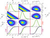 |
Fig. 2. Mosaic of |

where Ki−1 = ∫0+∞PDFPo.(θi) dθi is the normalization constant. Once the posterior PDFs for (k1M, λM, yiM) are obtained, the corresponding PDFs of the physical explosion parameters (E, Mej, R0) can be reconstructed by applying the inverse transformations of Eq. (7), as described in Appendix A.
It should be noted, however, that these posterior PDFs are derived in a univariate way (i.e., along single axes). This approach may underestimate modeling uncertainties, since off-axis correlations between parameters are not fully captured. For instance, inspection of the k1–λ plane reveals a non-negligible covariance, intrinsic to the model due to their product entering the normalized luminosity in Eq. (6). As illustrated by the difference between the CDFs along the axes and over the full space (Fig. 2), the broader multidimensional distributions highlight the need to account for covariance-driven uncertainties. To address this limitation, SUPERBAM employs a Monte Carlo (MC) procedure that randomly generates 104 triplets of modeling parameters (yi, λ, k1) around the HMC best-fit solution θM, fixing σ = σM. For each triplet, the posterior probability value is computed and used as a statistical weight, naturally decreasing with distance from the optimum. From this weighted sample of parameter triplets, expectation values and variances are derived for both the modeling parameters and, through the inverse transformations of Eq. (7), for the physical parameters (E, Mej, R0).
2.2. Validation test
To validate our approach, we apply SUPERBAM to the previously published LCs of SN 1987A (Catchpole et al. 1987), SN 2009E (Pastorello et al. 2012), and OGLE-14 (Terreran et al. 2017), shown in Fig. 1, and compare the results with the HM from Pumo & Zampieri (2011)’s post-explosive model (see Table 1 of Paper II, and references therein). As a consequence, the temporal sampling of the bolometric LCs reflects the reconstruction methods used in the original works and may slightly differ from that obtained with our own bolometric reconstruction technique (see also Sect. 3.1). Based on the procedure outlined in Section 2.1, SUPERBAM provides an initial estimate from the priors for E, Mej, R0, and MNi, as well as two posterior estimates of E, Mej, and R0 obtained through different approaches. The first, referred to as the posterior best model, corresponds to the parameter configuration that maximizes the posterior probability (i.e., the mode of the distribution), derived using the HMC sampler; the associated uncertainty is estimated from a univariate analysis of the posterior. The second, instead, is obtained through a MC simulation, yielding the mean values and standard deviations of the physical parameters over the multidimensional posterior support. These two posterior estimates are consistent with each other within their respective error bars, demonstrating SUPERBAM’s ability to converge toward coherent and more precise modeling results compared to those obtained from the priors through the scaling relations (see Table 1).
Results of the validation test.
As the output of SUPERBAM, we adopt the best-fit model obtained with the HMC-Sampler, while assigning uncertainties derived from the MC approach. This choice combines the advantage of a model that best reproduces the observed data with error estimates that account for multidimensional parameter correlations.
When comparing the SUPERBAM results with the HM, we find that the results are fully consistent within the errors, with the only exception of the energy for SN 2009E (about a factor two higher). This offset in the explosion energy is present in all SNe and it is especially evident for SN 2009E and OGLE-14. This systematic discrepancy can be traced back to the intrinsic assumptions of semi-analytic models. Indeed, unlike hydrodynamical simulations, our model adopts a uniform density profile for the ejecta. As already discussed in previous works, this simplification leads to an overestimate of the energy budget because more mass is effectively concentrated in the fast-moving outer layers, increasing the kinetic energy content. This behavior was noted for OGLE-14 by Terreran et al. (2017), where the semi-analytic model of Zampieri et al. (2003) yielded an explosion energy ∼70% larger than the HM estimate, precisely because the early acceleration phase of the ejecta is not accounted for. A similar result was reported for SN 2009E in Pastorello et al. (2012), where the same semi-analytic approach produced an Mej ∼ 26 M⊙ and an E ∼ 1.3 foe, again exceeding HM estimates due to the uniform density assumption. SUPERBAM mitigates part of this bias, as it accounts for the effect of 56Ni heating on the recombination process. As noted by Pastorello et al. (2012), neglecting the non-uniform distribution of 56Ni leads to an underestimate of its contribution at late photospheric phases, forcing the model to invoke a more massive envelope to sustain the recombination. By incorporating this effect, SUPERBAM achieves results that converge more closely to HM values, especially for the ejecta mass. Smaller differences are found in the initial radius. In our framework, the uniform-density assumption tends to confine the ejecta more tightly at early times, leading to slightly smaller radii than those inferred from HM. This discrepancy increases with ejecta mass, but in the case of OGLE-14 the results remain consistent within the error bars.
Finally, it is important to emphasize that the 56Ni mass derived by SUPERBAM from the LC tail (cf. Eq. (2)), corresponds to the amount of nickel present in the ejecta at late times. This represents a lower limit compared to HM results, which include the fraction of nickel that falls back onto the compact remnant. Consequently, our 56Ni masses are systematically lower than those obtained with HM. In summary, SUPERBAM offers a fast and physically consistent way to characterize 1987A-like SNe, providing results comparable to HM, while significantly reducing the computational time. This makes SUPERBAM particularly well suited for the analysis of large SN samples.
3. The sample of 87A-like SNe
Over the last two years, the number of published 87A-like SNe has nearly doubled, largely thanks to the efforts of wide-field surveys such as ZTF/CLU (Sit et al. 2023). In Paper I, a sample of 14 SNe 1987A-like was analyzed using the approach of scaling relations, relying on bolometric LCs and velocity data already available in the literature. In this work, we expand this sample to nearly double its size by homogeneously reconstructing the bolometric LCs, estimating line velocities and their pseudo-equivalent widths (pEWs) from peak spectra, and applying the SUPERBAM procedure to derive the physical properties at the explosion.
To this aim, we performed a systematic search through the literature of the past three decades, selecting the best-observed long-rising type II SNe according to the following criteria:
-
Multi-band photometric coverage (at least three filters) starting no later than
 d and extending through the end of the recombination phase (tf*) with at least one point on the 56Ni tail. This allows us to reconstruct the bolometric LC and constrain priors such as the 56Ni mass.
 -
Reliable estimates of distance (or redshift) and extinction are required. It is necessary to correct both spectra and photometry before deriving bolometric LCs and velocities.
Both SUPERBAM and alternative modeling approaches require these conditions to be applied; otherwise, the analysis cannot be considered reliable (e.g., Martinez & Bersten 2019). Following these criteria, we selected a sample of 28 long-rising type II SNe published before 2025. The list reported in Table 2 includes, for each of these events, the estimated explosion epoch (which is not a free parameter of the fit, but is fixed as the midpoint between the last non-detection and the discovery date), the host galaxy with its distance modulus, the adopted redshift, the total visual extinction, and the environmental metallicity in terms of oxygen abundance [12+log(O/H)], along with the main bibliographic references from which this information is taken.
Sample of 1987A-like SNe and key information used for the spectrophotometric analysis.
The collection of multi-band photometric data for each SN enables the reconstruction of their bolometric LCs. In addition to the datasets published in the references listed in Table 2, we also include, where available, photometry from the ATLAS (Asteroid Terrestrial-impact Last Alert System; see, e.g., Tonry et al. 2018). Spectroscopic data are gathered from the same cited works, selecting spectra obtained near the luminosity peak (see Table C.2 for acquisition dates and epochs of the spectra considered for each SN). These spectra are used to measure photospheric velocities and line equivalent widths, providing complementary constraints on the ejecta composition and kinematics. Although, no public spectra are available for SN 2021zj during the peak stage, its modeling was carried out by SUPERBAM using the full photometric scaling relations system in Eq. (4). However, this object is not included in the spectroscopic analysis made for the other 1987A-like SNe in the sample.
3.1. Bolometric luminosity
For the computation of bolometric luminosity, all available multi-band photometry from the literature has been re-analysed in a homogeneous way, ensuring a consistent procedure for the construction of bolometric LCs. In particular, we apply SUPERBOL procedure for the bolometric integration of the spectral energy distribution (SED) described by Nicholl (2018). In addition, the multi-band LCs are first reconstructed in time using GPR interpolation, and extrapolated under the constant-color assumption5. The use of GPR provides synthetic photometric points at missing epochs, effectively increasing the number of multi-band observations and allowing for virtually simultaneous coverage across filters6. This interpolation yields a denser bolometric sampling while preserving consistency with curves derived from real data within the uncertainties7. In addition to photometry, information on distance and extinction is required. For SNe with z > 0.01, distances are derived from the redshift, assuming ΩΛ = 0.685, ΩM = 0.315 and the Hubble-Lemaıtre constant equals to H0 = 67.4 km s−1 Mpc−1 (e.g., Planck Collaboration VI 2020). For nearby SNe, where peculiar motions can dominate over the Hubble flow, we adopt published distance moduli (Table 2). In the case of the gravitational lensed SN Refsdal, we also correct the observed flux for the magnification lens factor μ = 15 (e.g., Grillo et al. 2016, and references therein). The reddening correction is applied assuming the Cardelli et al. (1989) extinction law with RV = 3.1, appropriate for the diffuse interstellar medium. The color excess E(B − V), computed as the difference between observed and intrinsic colors, is then estimated from the total extinction as E(B − V) = AV/RV. Finally, no UV cut-off is applied to the SEDs. Although the early post-explosion phases (< 10–20 d) might be affected by a significant drop in the UV flux, this effect is negligible for SNe II because of the hydrogen-rich, metal-poor nature of their ejecta (e.g., Gezari et al. 2008; Bufano et al. 2009), and is irrelevant for our analysis, which does not rely on the earliest epochs. However, the SED fitting is potentially affected by line blanketing8.
The bolometric LCs obtained in this way are then used by SUPERBAM to constrain the physical parameters of the explosions (see Sect. 4). As a preparatory step, however, the procedure also measures key morphological features of the LCs, reported in Table C.1, such as MNi, tf* and LM (see left panels of Fig. 3). The distribution of nickel masses, directly inferred from the radioactive tails, spans nearly an order of magnitude, from the ∼0.04 M⊙ of SN 2009E up to the 0.4–0.5 M⊙ measured for OGLE-14 and SN 2021zj. Grouping the sample according to MNi highlights three main subsets. Events with MNi < 0.1 M⊙, including SN 1987A and SN Refsdal, cluster around peak luminosities of ∼1042 erg s−1 and recombination end times tf* ≈ 100–150 d. SNe with intermediate nickel masses (0.1–0.2 M⊙) reach higher peak luminosities, still consistent with the observed scaling, but in some cases show broader LCs, as for DES16C3cje, whose tf* exceeds 200 d. Finally, the most nickel-rich explosions (MNi > 0.2 M⊙) attain luminosities above 1043 erg s−1, with OGLE14-73 representing the event with the brightest and broadest peak of the class. SN 2021zj and SN 2020faa also belong to this group, though they display a slow pre-maximum rise, with tm ∼ 40–60 d, unlike OGLE14-73 where no early coverage is available. Across the entire sample, LM shows a linear increase with MNi, as illustrated in the left-up panel of Fig. 3. This trend has also been reported in broader samples of H-rich SNe (e.g., Martinez et al. 2022), and becomes particularly clear for 1987A-like SNe, in which the radioactive Ni-heating is more powerful than the ejecta recombination-cooling (i.e., where the Λ-term dominates; see Eqs. (67)–(68) in Paper II). However, events such as OGLE-14 and SN 2020faa exhibit luminosities significantly above the predicted trend, suggesting the contribution of additional energy sources that enhance the overall brightness. On the contrary, the same clear dependency on MNi is not observed for tf*, which is more influenced by other properties of the explosion, deriving from its link with the diffusion and ejecta expansion rates ( ; cf. Eq. (76) of Paper II).
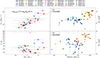 |
Fig. 3. Observational properties derived from the bolometric LCs and spectra of the SN sample. Top left: Distribution of the peak luminosity LM as a function of the 56Ni mass estimated from the radioactive tail fit. The trend line is obtained through a linear regression log10LM-log10MNi; the correlation is highly significant (p-value ≪ 0.01 and Pearson coefficient of 0.89). Bottom left: Distribution of tf* versus the 56Ni mass for the same SN sample. Top right: pEWs as a function of expansion velocities for the Hα and Fe II lines, for the SNe with available data. The color and shape of the markers follow the top legend, while the marker border indicates the line type according to the internal legend. Bottom right: Same as the top-right panel, but for the Hβ and Ba II lines. |
3.2. Spectroscopic features
The available SN spectra have been reduced and corrected for both reddening and redshift, thus placing them in the rest frame and recovering their intrinsic continuum shape. These corrections, applied consistently across the sample, allow a direct comparison of line profiles and velocities, providing essential constraints on the ejecta properties.
For this purpose, the deredden and dopcor tasks within the Image Reduction and Analysis Facility (IRAF; Tody 1986) are employed. After the corrections, the main absorption features typical of SNe 1987A-like are analyzed, with particular attention to the Balmer lines (Hα, Hβ) and metal lines such as Ba II-λ6142 and Fe II-λ5169. The minima of the P-Cygni absorption profiles are measured using Gaussian fits with the IRAF splot tool, in order to infer the expansion velocities from their Doppler shifts. Simultaneously, these fits provide the pEWs used to characterize line strengths and assess the relative contribution of different ions. The results of this analysis are summarized in Table C.2 and illustrated in the right panels of Fig. 3.
From a spectroscopic point of view, the majority of the SNe show broad P-Cygni Balmer profiles together with Fe II and Ba II features, which are particularly suited to trace the photospheric velocity. In our procedure, the photospheric velocity at peak (vM) adopted in the priors of SUPERBAM is taken from the Fe II velocity, which is available for the large majority of the sample. When Fe II is not detected, the Ba II velocity is used instead, and in the few cases where neither of these lines is measurable (e.g., SN Refsdal and SN 2020oem) the Hα velocity is employed, rescaled by a factor of 2 to account for the systematic offset between hydrogen and metal lines. Indeed, Balmer lines yield expansion velocities of 6000–9000 km s−1, systematically higher (by a factor of 1.5–2.5) than those derived from metal lines (2000–5000 km s−1). This difference originates from the fact that Balmer transitions are mostly shaped by photoionization and recombination processes in the outer ejecta layers, where the gas is only partially ionized and expands at higher velocities. Conversely, ionized metal lines require higher temperatures to sustain the proper ionization state, and become more prominent where the abundance of heavy elements is larger, i.e., in deeper and slower-moving regions of the photosphere. The smaller velocity offset between Hβ and Ba II supports this interpretation, since the Hβ formation region lies deeper than that of Hα and requires a higher excitation energy to populate the n = 4 level. Only a few objects deviate from these general trends, such as SN2009E and SN2005ci, which display unusually large offsets between Balmer and metal velocities.
As for pEWs, the Balmer lines generally exceed the strength of metal features by factors of 5–10. A noteworthy case is DES16C3cje, whose narrower Hα profile and weaker relative pEW suggest a non-standard post-explosion scenario (see also Gutiérrez et al. 2020). At peak phase, Fe II pEWs across the whole sample remain relatively uniform, typically in the range of 10–30 Å. In contrast, Ba II displays a much larger scatter, with values spanning from a few Å (e.g., SN 2018hna) up to ∼10 Å or more (e.g., SN 1987A and SN 2009E). Previous studies had suggested the existence of two distinct subgroups of 87A-like SNe based on Ba II strength (e.g., Takáts et al. 2016); however, in our extended sample the distribution appears more continuous, with several events occupying intermediate values.
In addition, a possible anti-correlation between the velocity of the Ba II line and its pEW is hinted at in our data. Although the statistical significance of this trend is limited (see Sect. 4.2), it can be interpreted in terms of the ejecta density structure. In more compact explosions, where the ejecta expand less rapidly, the higher density in the line-forming regions favors stronger Ba II absorption (cf. Mazzali & Chugai 1995). Within this framework, SNe with lower Ba II velocities during the peak phase are naturally expected to display deeper Ba II lines. While the spectra considered here are all collected around the recombination peak phase, variations in the location and temperature of the Ba II formation region can also affect this line strength (e.g., Xiang et al. 2023). A systematic investigation of spectrophotometric dependencies, including the role of physical parameters, is deferred to Sect. 4.2.
4. Modeling long-rising SNe with SUPERBAM
To explore the physical properties of the selected 1987A-like sample, we applied the SUPERBAM procedure to the entire set of objects. As discussed in Sect. 2, the pipeline provides estimates of the explosion energy, ejecta mass, and progenitor radius (summarized in Table C.3), as well as the synthesized 56Ni mass, the latter being directly constrained from the radioactive tail of the LC (Table C.1). By comparing the observed LCs with the simulated ones obtained from the models presented in Paper II and Popov (1993), and using the parameters derived by SUPERBAM through scaling relations and HMC sampling, we can evaluate both the physical parameter inference and the capability of these models to reproduce the observed bolometric evolution (Fig. 4).
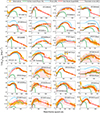 |
Fig. 4. Bolometric LC data for each SN in our sample. The name of each SN is indicated within its panel. The adopted explosion epochs (t = 0) are fixed from observational constraints (see Table 2). Along with the data, we present the synthetic LCs obtained from the analytical model described in Paper II. The parameters for these models were determined using the prior values given by the scaling relations, and the best-fit model obtained from SUPERBAM analysis. The shaded region marks the LCs associated with the explored parameters within the error ranges of the MC method. Data earlier than 30 days are not included in the fitting procedure. For comparison, the synthetic LC of the nickel-free model by Popov (1993) is also included, calculated for the best-model parameters. |
The Ni–free simulations of Popov (1993) systematically underestimate both the peak luminosity and the end of the recombination phase, owing to the absence of additional heating from radioactive 56Ni in the ejecta. A direct comparison between the Popov (1993) and Paper II models therefore allows us to quantify the role of 56Ni in shaping the LC morphology. Interestingly, this difference becomes progressively smaller in SNe with recombination onset later than ∼30 days, i.e., for progenitors with significantly larger initial radii (cf. Eq. (7)). As expected, the best-fit posterior models provide a significantly better agreement with the data compared to the priors, which generally capture the onset and termination of recombination but fail to accurately reproduce the luminous intensity.
Among the 28 SNe in the sample, ten show a reduced chi-squared9 (χν2) above unity, while the others are well fitted within the observational uncertainties. A first group of events, including SN1987A, SN1998A, SN2000cb, SN2004em, SN2006V, SN2009E, SN2009mw, SN2018hna, and SN2021aatd, shows excellent agreement between models and observations (i.e., χν2 ∼ 1), indicating that the automatic procedure robustly recovers the main LC features. For SN 2006V and SN 2018hna, however, the statistical agreement is formally poorer (reduced χν2 ∼ 2.3–2.7), mainly because the exceptionally dense UV–NIR multi-band coverage yields very small bolometric uncertainties (∼0.02 dex). Rescaling the log10-luminosity error to more typical values (0.05 dex) would bring the χν2 below unity, confirming the adequacy of the fit.
A second group, made by PTF12gcx, PTF12kso, DES16C3cje, SN 2018cub, SN 2018imj, SN 2020oem, SN 2020abah, SN 2021zj, SN 2021skm, and SN 2021wun, also yields apparently excellent fits. However, in some of these cases the error bars on the reconstructed bolometric flux are significantly large, that reduce the χν2 ≲ 0.5, limiting so the statistical robustness of the LC comparison and parameters inference.
Other SNe display discrepancies mainly due to limited temporal coverage or underestimated photometric errors. For instance, SN 2004ek, SN 2006au, and SN 2018ego suffer from sparse data and very small luminosity uncertainties, which drive the χν2 to high values (grater than 3) despite an overall model-consistent evolution. SN Refsdal is fairly well reproduced around peak luminosity, but the lack of late–time data prevents a reliable constraint on the end of recombination. In some cases, the models clearly overfit or misinterpret parts of the LC. SN 2005ci shows spurious overfitting of the early rise, while SN2019bsw and SN 2021mju suffer from noisy data that lead the procedure to confuse the late plateau with the onset of the tail, introducing large uncertainties in all explosive parameters.
The two most luminous events in the sample, OGLE-14 and SN 2020faa (LM ∼ 1043 erg s−1), both return reduced χν2 values well above unity, highlighting the difficulty of reproducing the entire peak solely through the contribution of radioactive 56Co. In OGLE-14, the higher χν2 value is mainly due to the deviation seen at the end of recombination, which could be explained by a different ejecta density structure or an additional energy source placed inside. For SN 2020faa, the deviation is further supported by a change of slope in the nebular tail, suggesting the presence of an additional power source. A plausible interpretation is energy input from a hidden shock–powered mechanism, possibly magnetar–driven (see also Salmaso et al. 2023), contributing to the luminosity at nebular phases. Interestingly, DES16C3cje also deviates from the expected 56Co decline rate and is instead compatible with the shallower slope expected from accretion–powered emission (Gutiérrez et al. 2020).
Finally, several SNe show an early–time luminosity excess (within ∼30 days of explosion) relative to the adopted model, which does not include contributions from thin-shell emission (see details in Paper II) or shock interaction with a dense CSM (e.g., Cosentino et al. 2025). Out of the 28 SNe analyzed, 13 exhibit this behavior, with particularly striking examples being SN2021zj and SN2021aatd. In SN2021zj, the interaction scenario is supported by the presence of narrow emission lines in the spectra (Jacobson-Galán et al. 2024), while in SN2021aatd no narrow features were detected beyond the first two days. However, the absence of narrow lines does not rule out CSM interaction as the underlying mechanism (e.g., Khatami & Kasen 2024, and references therein).
4.1. Physical properties of the 87A-like class
The physical parameters derived from the SUPERBAM modeling for the 1987A-like sample are listed in Table C.3. When considered as a whole, they reveal a rather heterogeneous population, with asymmetric distributions in explosion energy and 56Ni mass (see Fig. 5). In contrast, the distribution of ejecta masses is nearly symmetric, with the mean, median, and mode all close to ∼19 M⊙. Explosion energies and 56Ni masses, however, display a mode shifted toward lower values, with 8 SNe clustering below the sample averages. This points to the presence of two broad subgroups of 87A-like events: one characterized by modest energies (∼1.2 foe) and 56Ni masses around 0.07 M⊙ (including SN 1987A, SN 2009E, etc.), and another, more energetic, group peaking around 4 foe and 56Ni masses above 0.11 M⊙. About one quarter of the sample exhibits explosion energies exceeding 5 foe, reaching values that are difficult to reconcile with standard CC mechanisms (e.g., OGLE-14 and SN 2020faa).
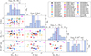 |
Fig. 5. Distribution of SNe physical properties. The diagonal panels show the histograms of the logarithm of each parameter (MNi, E, Mej, R), with the mean value (dashed line) and quartiles (25%, 50%, and 75%; see dotted lines) indicated. The lower triangular panels show scatter plots of the parameter pairs for each SN in the sample. |
By mapping energy, ejecta mass, and 56Ni together, the extended sample allows us to better outline the parameter space of 1987A-like SNe. The resulting distribution appears continuous, but still allows events to be broadly grouped into two categories: a high-E, high-56Ni subgroup with ejecta masses ≳20 M⊙ (e.g., OGLE-14), and another, more similar to SN 1987A, with lower ejecta masses (< 20 M⊙) and explosion energies spanning a wide range from ∼0.3 foe up to ∼2 foe, in line with the trends already reported in Paper I.
Similarly to ejecta masses, progenitor radii at the explosion time show a roughly symmetric distribution centered around (6 − 7)×1012 cm, but with two secondary tails: one at smaller radii of order 1012 cm, and another at larger radii, beyond 3 × 1013 cm. The low-radius tail includes events such as SN 2018ego, SN 2020oem, PTF12gcx, SN 2021mju, SN 2021skm, and SN 2021wun. However, these objects generally suffer from poor or noisy coverage in the early phases or near the end of recombination, which likely makes the radius estimates uncertain and possibly underestimated. Conversely, the high-radius tail contains several well-sampled and robustly modeled events (e.g., SN 2004em, SN 2004ek, OGLE-14, and SN 2021zj). Interestingly, the highest-radius events are also those with the largest explosion energies and 56Ni masses. Moreover, up to ∼7 × 1012 cm the 56Ni mass tends to decrease with increasing radius, reaching a minimum for SN 2009E, and then rises again for the most extended progenitors. This trend is consistent with the intrinsic nature of 1987A-like SN LC, where the slow rise of the second peak depends sensitively on the initial radius and on the 56Ni yield. This behavior further distinguishes the group with lower radii and energy from the more energetic and extended one, which would otherwise resemble standard SNe II were it not for their unusually high 56Ni content (average 56Ni mass for SN II population is ∼0.037 ± 0.005 M⊙; Rodríguez et al. 2021).
The extended parameter space inferred from our modeling also enables a qualitative comparison with recent stellar-evolution predictions for BSG progenitors. In particular, the inferred explosion energies and 56Ni masses follow the exponential trend expected from neutrino-driven explosion models (e.g., Schneider et al. 2025), while the broad range of ejecta masses and progenitor radii overlaps with those predicted by recent grids of pre-SN supergiant models (Schneider et al. 2024). However, most single-star models at solar metallicity struggle to produce sufficiently compact and massive blue supergiants, confirming that either lower metallicity evolution (e.g., Woosley 1988) or binary interaction and merger channels (e.g., Tsuna et al. 2025) may be required to explain the 1987A-like SNe. Moreover, the most energetic and 56Ni-rich events in our sample may also invite comparison with pair-instability progenitor models (e.g., Terreran et al. 2017), which naturally predict large explosion energies and nickel yields (e.g., Kasen et al. 2011; Dessart et al. 2012).
Finally, note that the explosion parameters derived by SUPERBAM are consistent with those obtained in other previous works (see Table 3 of Paper I, and references therein), confirming the reliability of our approach (see also Sect. 2.2). In Sect. 4.2, a detailed analysis of correlations among these physical parameters, as well as between the physical and spectrophotometric properties of the sample, is presented.
4.2. Correlations
To investigate possible statistical links between the explosion properties and the spectrophotometric features of the 1987A-like SN sample, we computed the Spearman correlation coefficient (ρc) and evaluated its significance with a t-test for each parameter combination (see Fig. 6). As already discussed in Sect. 3.1, the 56Ni mass correlates positively (ρc > 0) with the peak luminosity LM, with very high significance (p ≪ 0.01). MNi also shows a positive correlation with the explosion energy (p = 0.01), in agreement with theoretical expectations that link larger nickel yields to more energetic explosions (e.g., Schneider et al. 2025). From the spectroscopic side, MNi appears correlated with the Fe II line, both in velocity (p = 0.02) and in pEW (p = 0.02). Interestingly, higher nickel masses are associated with weaker Fe II absorption but faster line velocities. A possible interpretation is that larger amounts of 56Ni keep the recombination front and the photosphere at larger radii in the ejecta (see, e.g., Paper II), so that Fe II lines form in faster-moving layers where the Fe abundance is intrinsically lower. This effect would explain the counter-intuitive result that Ni-rich explosions show weaker Fe II features, not because of a reduced Fe content, but because the absorption originates in more external and less Fe-rich regions. Such behavior suggests that scaling relations for line velocities may need to explicitly account for the nickel mass. By contrast, the ejecta mass is strongly correlated with the recombination timescale tf*, as expected (Paper II), and shows a moderately significant trend with explosion energy (p = 0.03), but no direct correlation with 56Ni mass. Spectroscopically, Mej does not display connections with line properties.
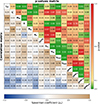 |
Fig. 6. Spearman correlation matrix for the physical and spectroscopic parameters considered. The lower-left half of squares show the Spearman correlation coefficient (ρc), color-coded from –1 (dark blue) to +1 (light brown), with the numerical values reported inside each cell. The upper-right half of squares show the associated p-values, color-coded according to significance level (from green for high significance to red for non–significant values). The diagonal reports the labels of the parameters. In addition to the parameters discussed in the previous sections, we also include [O/H] = 12+log(O/H) listed in Table 2. |
As anticipated in Sect. 3.2, line velocities are mutually correlated, as are velocity widths, with the exception of Ba II, which does not follow the same trends. In fact, Ba II shows a particularly peculiar behavior. An anti-correlation emerges between its velocity and pEW, which becomes statistically significant (p < 0.05) once clear outliers (e.g., DES16C3cje) are excluded. This trend is consistent with the idea that more compact explosions, with less extended ejecta, retain higher densities in the line-forming regions and therefore favor stronger Ba II absorption (e.g., Mazzali & Chugai 1995). In support of this interpretation, the modeling results indicate an additional correlation with the progenitor radius at explosion, which appears to be inversely related to the Ba II’s pEW. On the other hand, no correlation was found with other explosive parameters such as E and MNi. This suggests that the key factor regulating the intensity of the Ba II lines should be the compactness of the progenitors and ejecta, rather than differences in their nucleosynthetic production.
Progenitor radius also exhibits weak correlations with other parameters. In particular, an expected correlation between R0 and the oxygen abundance [O/H] of the host environment is present in our analysis (e.g., Taddia et al. 2013, 2016). Curiously, metallicity itself shows possible links with both peak luminosity and expansion velocity. SNe in more metal-rich environments tend to expand faster and peak at higher luminosities. Although the significance is low, these trend could provide insights into the role of metallicity in shaping the properties of 1987A-like events.
However we note that correlation does not imply causation. Moreover, although the present sample is significantly larger than in previous works, it could not constitute a fully unbiased representation of the 1987A-like population. Selection effects linked to discovery methods, survey strategies, and spectroscopic follow-up may introduce statistical biases that affect both distributions and correlations. These results should therefore be used with caution, although they will gain robustness as the number of well-observed 1987A-like SNe increases in the coming years.
5. Summary and further consideration
In this work we introduced the novel procedure SUPERBAM (Supernova Bayesian Analytic Modeling), a fast-modeling framework designed to infer the main physical properties of H-rich SNe from their bolometric LCs and spectroscopic information during the recombination phase. SUPERBAM relies on Bayesian statistics and analytical prescriptions, providing posterior distributions for explosion energy, ejecta mass, progenitor radius, and synthesized 56Ni mass. The method was validated against well-studied benchmarks and shown to reproduce the results of detailed numerical hydrodynamic simulations at a fraction of their computational cost.
We then applied SUPERBAM to the most comprehensive sample of 87A-like SNe assembled so far (28 events), reconstructing their bolometric LCs in a homogeneous way and measuring spectroscopic features at maximum. The analysis reveals a heterogeneous population that nevertheless clusters into two broad groups: (i) lower-energy explosions with modest 56Ni yields, reminiscent of SN 1987A, and (ii) more energetic events (sometimes exceeding 5 foe) with higher nickel production and, in some cases, unusually large progenitor radii. The parameter space, however, appears continuous, suggesting a spectrum of possible progenitor/explosion configurations rather than discrete categories.
From the statistical comparison of physical properties and spectrophotometric observables, we confirm the robust correlation between 56Ni mass and both peak luminosity and explosion energy, as well as the strong link between ejecta mass and recombination timescale. We also identify a peculiar behavior of Ba II, whose line strength anti-correlates with velocity and appears inversely related to progenitor radius. This suggests that the prominent Ba absorption observed in many 87A-like events arises primarily from progenitor compactness and ejecta density, rather than from enhanced nucleosynthetic production. Notably, for progenitors with radii approaching ∼1013 cm, the Ba II strength converges toward that of standard SNe II (pEWBa II ∼ 5 Å; cf. Gutiérrez et al. 2017), supporting the interpretation that compactness, and not abundance anomalies, could be the key driver. Future progress on this front will require detailed spectral synthesis calculations that account for the thermodynamical state of the ejecta (temperature and density), in order to disentangle abundance from excitation effects.
Finally, several events display luminosity components not fully reproduced by standard recombination plus 56Ni heating. The brightest SNe in our sample (e.g., OGLE-14 and SN 2020faa) require additional power sources such as magnetar spin-down or accretion, while others show early-time excesses consistent with interaction with CSM (e.g., SN 2021zj and SN 2021aatd). This highlights the need to extend fast-modeling frameworks similar to SUPERBAM to incorporate non-radioactive energy sources and CSM interaction, in order to capture the full diversity of 87A-like explosions. In particular, the inclusion of CSM-related components would allow us to constrain not only the explosion parameters but also the physical properties of the surrounding material. Combined with detailed spectroscopic analysis, this approach would provide key insights into the progenitor mass-loss history and the pre-explosion evolution leading to events such as SN 2021zj. A dedicated study of this object, including unpublished spectroscopic observations, is planned for future work.
The development of such efficient, Bayesian-based procedures is particularly timely in view of ongoing and upcoming large surveys (e.g., ZTF and LSST), which will discover thousands of peculiar SNe. SUPERBAM represents a step toward scalable analysis pipelines, able to rapidly characterize large samples with improved accuracy over simple scaling relations and at a fraction of the cost of full numerical simulations. Moreover, our framework has proven effective even in the absence of spectroscopic information, providing physically meaningful estimates based solely on photometric data. This feature is particularly valuable for next-generation surveys, which will deliver extensive multi-band photometry but limited spectroscopic coverage. In this way, this work opens the path for systematic population studies of rare transients, bridging the gap between survey data and detailed physical modeling.
Acknowledgments
We acknowledge support from the Piano di Ricerca di Ateneo UNICT – Linea 2 PIA.CE.RI. 2024–2026 of Catania University (project AstroCosmo, P.I. A. Lanzafame). CI gratefully acknowledges the support received from the MERAC Foundation. SPC thanks Cardiff University for hosting him during the research activities that contributed to this work.
References
- Arnett, W. D. 1980, ApJ, 237, 541 [Google Scholar]
- Arnett, D. 1996, Supernovae and Nucleosynthesis: An Investigation of the History of Matter from the Big Bang to the Present (Princeton University Press) [Google Scholar]
- Arnett, W. D., Bahcall, J. N., Kirshner, R. P., & Woosley, S. E. 1989, ARA&A, 27, 629 [NASA ADS] [CrossRef] [Google Scholar]
- Ashour, S. K., & Abdel-hameed, M. A. 2010, J. Adv. Res., 1, 341 [Google Scholar]
- Bellm, E. C., Kulkarni, S. R., Graham, M. J., et al. 2018, PASP, 131, 018002 [Google Scholar]
- Bersten, M. C., Benvenuto, O., & Hamuy, M. 2011, ApJ, 729, 61 [NASA ADS] [CrossRef] [Google Scholar]
- Bianco, F. B., Ivezić, Ž., Jones, R. L., et al. 2021, ApJS, 258, 1 [Google Scholar]
- Bufano, F., Immler, S., Turatto, M., et al. 2009, ApJ, 700, 1456 [NASA ADS] [CrossRef] [Google Scholar]
- Burrows, A. 1990, Ann. Rev. Nucl. Part. Sci., 40, 181 [Google Scholar]
- Cardelli, J. A., Clayton, G. C., & Mathis, J. S. 1989, ApJ, 345, 245 [Google Scholar]
- Catchpole, R., Menzies, J., Monk, A., et al. 1987, MNRAS, 229, 15P [NASA ADS] [CrossRef] [Google Scholar]
- Chatzopoulos, E., Wheeler, J. C., & Vinko, J. 2012, ApJ, 746, 121 [Google Scholar]
- Colgan, S. W. J., Haas, M. R., Erickson, E. F., Lord, S. D., & Hollenbach, D. J. 1994, ApJ, 427, 874 [Google Scholar]
- Cook, D. O., Kasliwal, M. M., Sistine, A. V., et al. 2019, ApJ, 880, 7 [Google Scholar]
- Cosentino, S. P. 2024, Ph.D. Thesis, Università degli Studi di Catania [Google Scholar]
- Cosentino, S. P., Pumo, M. L., & Cherubini, S. 2025, MNRAS, 540, 2894 [Google Scholar]
- Dessart, L., Waldman, R., Livne, E., Hillier, D. J., & Blondin, S. 2012, MNRAS, 428, 3227 [Google Scholar]
- Dexter, J., & Kasen, D. 2013, ApJ, 772, 30 [NASA ADS] [CrossRef] [Google Scholar]
- Fang, Q., Maeda, K., Ye, H., Moriya, T. J., & Matsumoto, T. 2024, ApJ, 978, 35 [Google Scholar]
- Gezari, S., Dessart, L., Basa, S., et al. 2008, ApJ, 683, L131 [NASA ADS] [CrossRef] [Google Scholar]
- Graham, M. J., Kulkarni, S. R., Bellm, E. C., et al. 2019, PASP, 131, 078001 [Google Scholar]
- Grillo, C., Karman, W., Suyu, S. H., et al. 2016, ApJ, 822, 78 [Google Scholar]
- Gutiérrez, C. P., Anderson, J. P., Hamuy, M., et al. 2017, ApJ, 850, 90 [CrossRef] [Google Scholar]
- Gutiérrez, C. P., Sullivan, M., Martinez, L., et al. 2020, MNRAS, 496, 95 [CrossRef] [Google Scholar]
- Inserra, C., Smartt, S. J., Jerkstrand, A., et al. 2013, ApJ, 770, 128 [NASA ADS] [CrossRef] [Google Scholar]
- Inserra, C., Prajs, S., Gutierrez, C. P., et al. 2018, ApJ, 854, 175 [NASA ADS] [CrossRef] [Google Scholar]
- Jacobson-Galán, W. V., Dessart, L., Davis, K. W., et al. 2024, ApJ, 970, 189 [CrossRef] [Google Scholar]
- Kasen, D., & Bildsten, L. 2010, ApJ, 717, 245 [NASA ADS] [CrossRef] [Google Scholar]
- Kasen, D., & Woosley, S. E. 2009, ApJ, 703, 2205 [NASA ADS] [CrossRef] [Google Scholar]
- Kasen, D., Woosley, S. E., & Heger, A. 2011, ApJ, 734, 102 [NASA ADS] [CrossRef] [Google Scholar]
- Kelly, P. L., Brammer, G., Selsing, J., et al. 2016, ApJ, 831, 205 [NASA ADS] [CrossRef] [Google Scholar]
- Khatami, D. K., & Kasen, D. N. 2019, ApJ, 878, 56 [NASA ADS] [CrossRef] [Google Scholar]
- Khatami, D. K., & Kasen, D. N. 2024, ApJ, 972, 140 [NASA ADS] [CrossRef] [Google Scholar]
- Kleiser, I. K. W., Poznanski, D., Kasen, D., et al. 2011, MNRAS, 415, 372 [Google Scholar]
- Lyman, J. D., Bersier, D., & James, P. A. 2014, MNRAS, 437, 3848 [Google Scholar]
- Martinez, L., & Bersten, M. C. 2019, A&A, 629, A124 [NASA ADS] [CrossRef] [EDP Sciences] [Google Scholar]
- Martinez, L., Anderson, J. P., Bersten, M. C., et al. 2022, A&A, 660, A42 [NASA ADS] [CrossRef] [EDP Sciences] [Google Scholar]
- Matsumoto, T., Metzger, B. D., & Goldberg, J. A. 2025, ApJ, 978, 56 [Google Scholar]
- Mazzali, P. A., & Chugai, N. N. 1995, A&A, 303, 118 [NASA ADS] [Google Scholar]
- Müller, T., Prieto, J. L., Pejcha, O., & Clocchiatti, A. 2017, ApJ, 841, 127 [Google Scholar]
- Nicholl, M. 2018, Res. Notes AAS, 2, 230 [NASA ADS] [CrossRef] [Google Scholar]
- Nicholl, M., Guillochon, J., & Berger, E. 2017, ApJ, 850, 55 [NASA ADS] [CrossRef] [Google Scholar]
- Orlando, S., Miceli, M., Pumo, M. L., & Bocchino, F. 2015, ApJ, 810, 168 [NASA ADS] [CrossRef] [Google Scholar]
- Pastorello, A., Baron, E., Branch, D., et al. 2005, MNRAS, 360, 950 [CrossRef] [Google Scholar]
- Pastorello, A., Pumo, M. L., Navasardyan, H., et al. 2012, A&A, 537, A141 [NASA ADS] [CrossRef] [EDP Sciences] [Google Scholar]
- Planck Collaboration VI. 2020, A&A, 641, A6 [NASA ADS] [CrossRef] [EDP Sciences] [Google Scholar]
- Popov, D. V. 1993, ApJ, 414, 712 [NASA ADS] [CrossRef] [Google Scholar]
- Pumo, M. L., & Cosentino, S. P. 2025, MNRAS, 538, 223 (Paper II) [Google Scholar]
- Pumo, M. L., & Zampieri, L. 2011, ApJ, 741, 41 [NASA ADS] [CrossRef] [Google Scholar]
- Pumo, M. L., & Zampieri, L. 2013, MNRAS, 434, 3445 [Google Scholar]
- Pumo, M. L., Turatto, M., Botticella, M. T., et al. 2009, ApJ, 705, L138 [NASA ADS] [CrossRef] [Google Scholar]
- Pumo, M. L., Cosentino, S. P., Pastorello, A., et al. 2023, MNRAS, 521, 4801 (Paper I) [CrossRef] [Google Scholar]
- Pun, C. S. J., Kirshner, R. P., Sonneborn, G., et al. 1995, ApJS, 99, 223 [NASA ADS] [CrossRef] [Google Scholar]
- Roberts, S., Osborne, M., Ebden, M., et al. 2013, Phil. Trans. R. Soc. A: Math. Phys. Eng. Sci., 371, 20110550 [Google Scholar]
- Rodríguez, Ó., Meza, N., Pineda-García, J., & Ramirez, M. 2021, MNRAS, 505, 1742 [CrossRef] [Google Scholar]
- Salmaso, I., Cappellaro, E., Tartaglia, L., et al. 2023, A&A, 673, A127 [NASA ADS] [CrossRef] [EDP Sciences] [Google Scholar]
- Schlafly, E. F., & Finkbeiner, D. P. 2011, ApJ, 737, 103 [Google Scholar]
- Schneider, F. R. N., Podsiadlowski, P., & Laplace, E. 2024, A&A, 686, A45 [NASA ADS] [CrossRef] [EDP Sciences] [Google Scholar]
- Schneider, F. R. N., Laplace, E., & Podsiadlowski, P. 2025, A&A, 700, A253 [NASA ADS] [CrossRef] [EDP Sciences] [Google Scholar]
- Silva-Farfán, J., Förster, F., Moriya, T. J., et al. 2024, ApJ, 969, 57 [Google Scholar]
- Singh, A., Sahu, D. K., Anupama, G. C., et al. 2019, ApJ, 882, L15 [Google Scholar]
- Sit, T., Kasliwal, M. M., Tzanidakis, A., et al. 2023, ApJ, 959, 142 [NASA ADS] [CrossRef] [Google Scholar]
- Smartt, S. J. 2009, ARA&A, 47, 63 [NASA ADS] [CrossRef] [Google Scholar]
- Smith, K. W., Fulton, M., Gillanders, J., et al. 2021, TNS AstroNote, 14, 1 [Google Scholar]
- Szalai, T., Könyves-Tóth, R., Nagy, A. P., et al. 2024, A&A, 690, A17 [Google Scholar]
- Taddia, F., Stritzinger, M. D., Sollerman, J., et al. 2012, A&A, 537, A140 [NASA ADS] [CrossRef] [EDP Sciences] [Google Scholar]
- Taddia, F., Sollerman, J., Razza, A., et al. 2013, A&A, 558, A143 [NASA ADS] [CrossRef] [EDP Sciences] [Google Scholar]
- Taddia, F., Sollerman, J., Fremling, C., et al. 2016, A&A, 588, A5 [NASA ADS] [CrossRef] [EDP Sciences] [Google Scholar]
- Takáts, K., Pignata, G., Bersten, M., et al. 2016, MNRAS, 460, 3447 [CrossRef] [Google Scholar]
- Terreran, G., Pumo, M. L., Chen, T. W., et al. 2017, Nature, 1, 713 [Google Scholar]
- Tody, D. 1986, SPIE Conf. Ser., 627, 733 [Google Scholar]
- Tonry, J. L., Denneau, L., Heinze, A. N., et al. 2018, PASP, 130, 064505 [Google Scholar]
- Tsuna, D., Fuller, J., & Lu, W. 2025, arXiv e-prints [arXiv:2508.21116] [Google Scholar]
- Turatto, M., Benetti, S., & Pastorello, A. 2007, AIP Conf. Ser., 937, 187 [Google Scholar]
- Utrobin, V. P., & Chugai, N. N. 2011, A&A, 532, A100 [NASA ADS] [CrossRef] [EDP Sciences] [Google Scholar]
- Utrobin, V. P., Wongwathanarat, A., Janka, H.-T., et al. 2021, ApJ, 914, 4 [NASA ADS] [CrossRef] [Google Scholar]
- Villar, V. A., Guillochon, J., Berger, E., et al. 2017, ApJ, 851, L21 [Google Scholar]
- Woosley, S. E. 1988, ApJ, 330, 218 [Google Scholar]
- Woosley, S. E., Heger, A., & Weaver, T. A. 2002, Rev. Mod. Phys., 74, 1015 [NASA ADS] [CrossRef] [Google Scholar]
- Xiang, D., Wang, X., Zhang, X., et al. 2023, MNRAS, 520, 2965 [NASA ADS] [CrossRef] [Google Scholar]
- Yang, S., Sollerman, J., Chen, T. W., et al. 2021, A&A, 646, A22 [NASA ADS] [CrossRef] [EDP Sciences] [Google Scholar]
- Young, T. R. 2004, ApJ, 617, 1233 [NASA ADS] [CrossRef] [Google Scholar]
- Zampieri, L., Pastorello, A., Turatto, M., et al. 2003, MNRAS, 338, 711 [NASA ADS] [CrossRef] [Google Scholar]
The GPR is a nonparametric supervised learning method used to solve regression problems. The GPR assumes that the N observed variables L = (L1, …, LN)T are randomly drawn from a multivariate Gaussian distribution f(m, K), where m = (μ1, …μN)T is the mean vector for each variable and K is their covariance matrix (NxN), also called kernel (Roberts et al. 2013). A GPR is hence specified by its mean function and kernel (see, e.g., Inserra et al. 2018).
For a complete list of explored kernels, see also GPR MATLAB Documentation..
The first two scaling equations in Eq. (3) are the same as in Eq. (4) of Paper I, while the third replaces Eq. (15) of the same work. Instead of relying on Lmin, tM, and vM, it directly relates the progenitor radius to tm, based on the proportionality derived in their Eq. (9). This assumes that ti (the onset of recombination) coincides with the pre-peak luminosity minimum. Although Paper II has shown that this is not always strictly valid (particularly in cases where a thin shell or CSM interaction modifies the early luminosity) this relation is nonetheless simple and robust enough to provide useful prior information on R0, while allowing sufficient flexibility for posterior inference.
The HMC algorithm is a Markov Chain Monte Carlo technique that generates random samples to efficiently explore and maximize a multi-parametric distribution. See also the MatLab documentation for details.
The constant-color refers to a temporal extrapolation technique in which missing-band fluxes are estimated by preserving the color difference measured at the nearest epoch with multi-band coverage (see Nicholl 2018).
In wide-field surveys (e.g., LSST), multi-band photometry is typically obtained on different nights, depending on the observing strategy (Bianco et al. 2021). In such cases, GPR is particularly effective.
See also Fig. 4.2 in Cosentino (2024).
As in normal Type II SNe, the SEDs of 1987A-like events can be affected by line blanketing in the blue bands (e.g., Kasen & Woosley 2009; Pastorello et al. 2012). We verified that recomputing the bolometric LC of SN 1987A with and without the U and B bands leads to differences of ∼5–20%, comparable to the intrinsic uncertainties of the blackbody fitting procedure. Bolometric LCs obtained by integrating all available bands and extrapolating to missing regions using a blak-body fit provide robust estimates of the total emergent luminosity (e.g., Lyman et al. 2014; Taddia et al. 2016).
The reduced chi–squared is defined as
![Mathematical equation: $$ \chi ^2_\nu =\nu ^{-1} \times \sum _{\rm Obs.} \left[\left(L^\mathrm{Obs.}_{\rm Bol.} - L^\mathrm{Mod.}\right)/\Delta L^\mathrm{Obs.}_{\rm Bol.} \right]^2, $$](/articles/aa/full_html/2026/03/aa57860-25/aa57860-25-eq36.gif)
where ν = NObs. − 4 is the freedom degree depending on the number of bolometric observations NObs. after 30d since explosion, the sum is extended on these observed data ( ,
,  ), and LMod. are the corresponding model bolometric luminosities at tObs..
Appendix A: Probability distribution function
This appendix describes the procedure adopted to construct and transform the probability distributions used in SUPERBAM for both the prior and posterior inference. This process involves two main steps: (1) defining the PDFs associated with the measured spectrophotometric features, and (2) converting the distributions of both measured features and modeling parameters into PDFs for the SN physical properties through the scaling relations.
As described in Sect. 2.1.1, once the key observables mi = {tm, tM, LM, vM, MNi} are measured, each with corresponding upper (mi+) and lower (mi−) uncertainties, a continuous probability distribution must be assigned to each feature. To achieve this, SUPERBAM models each observable as a random variable following a skew-normal distribution (e.g., Ashour & Abdel-hameed 2010), which accounts for possible asymmetries in the measurement errors:
![Mathematical equation: $$ f_0(x) = \frac{2}{\omega \sqrt{2\pi }} \exp \!\left[-\frac{(x-\xi )^2}{2\omega ^2}\right] \int _{-\infty }^{\alpha \left(\frac{x-\xi }{\omega }\right)} \frac{1}{\sqrt{2\pi }}\, e^{-\frac{t^2}{2}}\, dt. $$](/articles/aa/full_html/2026/03/aa57860-25/aa57860-25-eq39.gif)
The free parameters of the distribution (ω, ξ, and α) are determined so that the resulting mean, standard deviation, and skewness reproduce the measured central value and asymmetric uncertainties of each feature. In practice, we adopt the following punctual distribution assumptions based on the measured feature and its upper and lower uncertainties: the mode is set to A = mi, the mean to B = (2mi + mi+ + mi−)/4, and the standard deviation to C = (mi+ − mi−)/2. Under these assumptions, the shape parameter α is obtained by numerically solving the implicit relation (e.g., Ashour & Abdel-hameed 2010):
![Mathematical equation: $$ \frac{(4 - \pi )\times \delta ^3(\alpha )}{2[1 - \delta ^2(\alpha )]^{3/2}} + \mathrm{sign} (\alpha )\, \frac{\exp [-2\pi / |\alpha |]}{1 - \delta ^2(\alpha )} = \frac{2(B-A)}{C}, $$](/articles/aa/full_html/2026/03/aa57860-25/aa57860-25-eq40.gif)
where δ2(α) = 2α2/[π (1 + α2)]. Once α is known, the other PDF’s parameters are computed as:
These relations ensure that the resulting skew-normal function accurately reproduces the observed asymmetry in the measurement uncertainties (see also Fig. 3.12 in Cosentino 2024).
Since all the measured features represent intrinsically positive quantities, their probability density must also be defined on a positive domain. However, the standard skew-normal distribution f0(x) is defined over the entire real line and thus allows non-physical (negative) values. To prevent this issue and ensure continuity at the origin, we introduce a corrective function that smoothly suppresses the probability below zero while preserving the original distribution shape for positive values:
![Mathematical equation: $$ \begin{aligned} f(x) = N\times f_0(x)\times {\left\{ \begin{array}{ll} \exp \left[-\frac{x_0^2}{(x_0-\xi )^2}(x-\xi )^2/x^2\right]\,&x>0\\ 0\,&x\le 0 \end{array}\right.}, \end{aligned} $$](/articles/aa/full_html/2026/03/aa57860-25/aa57860-25-eq42.gif)
where x0 is related to the lowest admitted value and N is a normalization constant. This correction maintains the position of the distribution maximum and reproduces the original skew-normal behavior for x > x0.
As described in Sects. 2.1.1 and 2.1.3, the scaling relations provide a direct link between the observed features and the prior distributions of the physical parameters (E, Mej, R0), as well as between the model parameters (yi, λ, k1). Similarly, the posterior PDFs of the model parameters are related to the physical ones by applying the inverse transformations of the system described in Eq. 7.
In both cases, these transformations rely on the combination of independent random variables associated with the measured or inferred quantities. The operations between the involved PDFs can be reduced to two basic types:
-
Power operations – Let Y = Xα, with k ∈ ℝ and X > 0 a random variable defined on a positive support with PDF f(x). Then Y is also a positive random variable, whose PDF is given by
-
Product operations – Let Z = X Y, where both X > 0 and Y > 0 are independent random variables with PDFs f(x) and g(y), respectively. Then Z is also defined on a positive support, with the following PDF:
Since all variables involved in Eqs. 3 (or 4) and 10 are defined on a positive domain and independent, the combination of their PDFs can be performed using previous transformations.
Appendix B: Effects of 56Ni mixing
In this appendix, we investigate the effects of varying the 56Ni mixing parameter k2, or equivalently the characteristic radius xc, on the spatial distribution of radioactive material and on the resulting bolometric LC. This analysis is motivated by recent 3D simulations of SN 1987A (e.g., Utrobin et al. 2021), which predict significant outward mixing of 56Ni.
Within our analytical framework, the 56Ni distribution is described by an exponential profile characterized by the parameter xc, defined such that 95% of the total nickel mass is enclosed within a comoving radius xcRej (see also Eqs. 27-29 of Paper II):
![Mathematical equation: $$ \begin{aligned} x_c=\root 3 \of {\frac{\log {\left[0.05+0.95\times \exp {(-k_2)}\right]}}{k_2}}. \end{aligned} $$](/articles/aa/full_html/2026/03/aa57860-25/aa57860-25-eq45.gif) (B.1)
(B.1)
The fiducial value adopted in this work, k2 = 32.87 → xc = 0.45, is consistent with previous hydrodynamical models used for validation (Pumo & Zampieri 2011, 2013) and with classical prescriptions for nickel mixing (Young 2004).
Figure B.1 shows the mass fraction of 56Ni as a function of ejecta shell velocity for the SN 1987A best-fit model, computed for different values of xc and assuming comoving ejecta expansion. For the fiducial case (xc = 0.45), less than 0.01% of the nickel mass reaches velocities above ∼2500 km s−1, slightly below the maximum velocities inferred from observations (e.g., Colgan et al. 1994) and from 3D simulations (Utrobin et al. 2021). This difference can be partly attributed to the simplified density structure assumed in the analytical model, which adopts a uniform ejecta density, unlike hydrodynamical models where the outer layers are less dense and expand at higher velocities (cf. Section 2.2). Increasing the mixing parameter to xc = 0.55 results in a more extended nickel distribution with maximum velocities of around 3000 km s−1, comparable to those measured by Colgan et al. (1994).
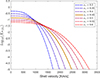 |
Fig. B.1. Abundance distribution of 56Ni inside the ejecta shells as a function of shell velocity. Different curves refers to EXP-56Ni distribution with different confinement coefficient xc (Paper II). |
Figure B.2 compares the bolometric LCs obtained for different values of xc. A less confined nickel distribution leads to a modest anticipation of the end of the recombination phase, with tf shifting from ∼112 days (xc = 0.45) to ∼108 days (xc = 0.55), while remaining fully consistent within the observational uncertainties. In order to evaluate the effect of 56Ni mixing on the physical parameters estimation, we further reapply the SUPERBAM fitting procedure using xc = 0.55 (corresponding to k2 = 18). The resulting best-fit parameters are very similar to those obtained for the fiducial case, with all parameters remaining unchanged within uncertainties, except for a modest increase in the ejecta mass from ∼17 M⊙ to ∼19 M⊙. This confirms that variations in the 56Ni mixing parameter mainly induce second-order effects on the inferred physical properties, in agreement with what reported in Paper II and previous studies (e.g., Pumo & Zampieri 2013). We stress, however, that a more detailed photometric investigation of mixing effects critically relies on having accurate observations of the late recombination phase (immediately preceding the onset of the radioactive tail), where the impact of different mixing configurations becomes more pronounced.
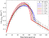 |
Fig. B.2. Effect of different 56Ni mixing on the bolometric LC for SN 1987A. |
Appendix C: Observational features and modeling
This appendix presents the main observational and modeling information for the 1987A-like SNe analysed in this work.
Tab. C.1 summarizes the key photometric observables derived from the bolometric LCs, followed by Tab. C.2 reporting the spectral measurements (photospheric velocities and pseudo-equivalent widths) obtained from the published spectra (see also Tab. 2 and references therein). Tab. C.3 contains the physical parameters inferred through our SUPERBAM analysis.
Bolometric LC features of the 1987A-like SN sample.
Main spectroscopic features of the 1987A-like SN sample.
Physical parameters of the 1987A-like SN sample derived by SUPERBAM procedure.
All Tables
Sample of 1987A-like SNe and key information used for the spectrophotometric analysis.
Physical parameters of the 1987A-like SN sample derived by SUPERBAM procedure.
All Figures
|
Fig. 1. Application of GPR to the bolometric LCs of SN 1987A, SN 2009E, and OGLE-14 taken from the literature (see Ref. in Sect. 2.2) to identify the main LC features. The adopted GPR employs a constant mean function combined with a Matérn 3/2 kernel. For each SN LC, the key epochs tm, |
| In the text | |
|
Fig. 2. Mosaic of |
| In the text | |
|
Fig. 3. Observational properties derived from the bolometric LCs and spectra of the SN sample. Top left: Distribution of the peak luminosity LM as a function of the 56Ni mass estimated from the radioactive tail fit. The trend line is obtained through a linear regression log10LM-log10MNi; the correlation is highly significant (p-value ≪ 0.01 and Pearson coefficient of 0.89). Bottom left: Distribution of tf* versus the 56Ni mass for the same SN sample. Top right: pEWs as a function of expansion velocities for the Hα and Fe II lines, for the SNe with available data. The color and shape of the markers follow the top legend, while the marker border indicates the line type according to the internal legend. Bottom right: Same as the top-right panel, but for the Hβ and Ba II lines. |
| In the text | |
|
Fig. 4. Bolometric LC data for each SN in our sample. The name of each SN is indicated within its panel. The adopted explosion epochs (t = 0) are fixed from observational constraints (see Table 2). Along with the data, we present the synthetic LCs obtained from the analytical model described in Paper II. The parameters for these models were determined using the prior values given by the scaling relations, and the best-fit model obtained from SUPERBAM analysis. The shaded region marks the LCs associated with the explored parameters within the error ranges of the MC method. Data earlier than 30 days are not included in the fitting procedure. For comparison, the synthetic LC of the nickel-free model by Popov (1993) is also included, calculated for the best-model parameters. |
| In the text | |
|
Fig. 5. Distribution of SNe physical properties. The diagonal panels show the histograms of the logarithm of each parameter (MNi, E, Mej, R), with the mean value (dashed line) and quartiles (25%, 50%, and 75%; see dotted lines) indicated. The lower triangular panels show scatter plots of the parameter pairs for each SN in the sample. |
| In the text | |
|
Fig. 6. Spearman correlation matrix for the physical and spectroscopic parameters considered. The lower-left half of squares show the Spearman correlation coefficient (ρc), color-coded from –1 (dark blue) to +1 (light brown), with the numerical values reported inside each cell. The upper-right half of squares show the associated p-values, color-coded according to significance level (from green for high significance to red for non–significant values). The diagonal reports the labels of the parameters. In addition to the parameters discussed in the previous sections, we also include [O/H] = 12+log(O/H) listed in Table 2. |
| In the text | |
|
Fig. B.1. Abundance distribution of 56Ni inside the ejecta shells as a function of shell velocity. Different curves refers to EXP-56Ni distribution with different confinement coefficient xc (Paper II). |
| In the text | |
|
Fig. B.2. Effect of different 56Ni mixing on the bolometric LC for SN 1987A. |
| In the text | |
Current usage metrics show cumulative count of Article Views (full-text article views including HTML views, PDF and ePub downloads, according to the available data) and Abstracts Views on Vision4Press platform.
Data correspond to usage on the plateform after 2015. The current usage metrics is available 48-96 hours after online publication and is updated daily on week days.
Initial download of the metrics may take a while.