| Issue |
A&A
Volume 707, March 2026
|
|
|---|---|---|
| Article Number | A368 | |
| Number of page(s) | 13 | |
| Section | Cosmology (including clusters of galaxies) | |
| DOI | https://doi.org/10.1051/0004-6361/202557927 | |
| Published online | 19 March 2026 | |
Combined LOFAR-uGMRT analysis of the diffuse radio emission in the massive clusters Abell 773 and Abell 1351
1
Istituto Nazionale di Astrofisica (INAF) – Istituto di Radioastronomia (IRA), via Gobetti 101, 40129 Bologna, Italy
2
Dipartimento di Fisica e Astronomia (DIFA), Universitá di Bologna, via Gobetti 93/2, 40129 Bologna, Italy
3
Istituto Nazionale di Astrofisica – Istituto di Astrofisica Spaziale e Fisica Cosmica (IASF), Via A. Corti 12, 20133 Milano, Italy
4
Hamburger Sternwarte, Universität Hamburg, Gojenbergsweg 112, 21029 Hamburg, Germany
5
Center for Radio Astronomy Techniques and Technologies, Rhodes University, Grahamstown 6140, South Africa
6
Leiden Observatory, Leiden University, PO Box 9513, 2300 RA Leiden, The Netherlands
7
Max-Planck-Institut für Extraterrestrische Physik (MPE), Gießenbachstraße 1, D-85748 Garching bei München, Germany
8
National Centre for Radio Astrophysics, Tata Institute of Fundamental Research, S. P. Pune University Campus, Ganeshkhind, Pune 411007, India
9
University of Kashmir, Hazratbal, Srinagar, J&K 190006, India
10
Manipal Centre for Natural Sciences, Manipal Academy of Higher Education, Karnataka, Manipal 576104, India
11
Indian Institute of Technology Indore, Indore, 453552 M.P., India
⋆ Corresponding author: This email address is being protected from spambots. You need JavaScript enabled to view it.
Received:
31
October
2025
Accepted:
17
January
2026
Abstract
Context. Radio halos are diffuse megaparsec-scale nonthermal radio sources located at the center of galaxy clusters. They trace relativistic particles and magnetic fields in the intra-cluster medium. The source of energy for their formation is believed to be the merging of galaxy clusters, which generates turbulence and reaccelerates aged electrons.
Aims. We studied the diffuse radio emission, spectral properties, and the connection between thermal and nonthermal emission in the massive (M500 ∼ 7 × 10¹⁴ M⊙), dynamically disturbed galaxy clusters Abell 773 and Abell 1351.
Methods. We combined observations from the LOFAR Two-meter Sky Survey Data Release 2 at 144 MHz and the new upgraded Giant Meterwave Radio Telescope at 650 MHz for both clusters. Archival XMM-Newton X-ray images were utilized to supplement our analysis.
Results. We confirm that both clusters host a radio halo, each of which has a largest linear size of ∼2 Mpc. We measure an integrated spectral index ( ) of ∼ − 1.0 for both clusters. Via point-to-point analysis, we show that the radio halo in A773 resembles a classical radio halo that follows a sublinear relation between radio and X-ray surface brightness. Conversely, A1351 exhibits a more complex and asymmetric radio halo that is embedded with several radio sources, including the brightest cluster galaxy, a tail galaxy, and the ridge. We find a deviation from the sublinear relation in the point-to-point analysis that is due to the presence of these contaminating radio sources.
Key words: radiation mechanisms: non-thermal / galaxies: clusters: intracluster medium / galaxies: clusters: individual: A773 / galaxies: clusters: individual: A1351
© The Authors 2026
 Open Access article, published by EDP Sciences, under the terms of the Creative Commons Attribution License (https://creativecommons.org/licenses/by/4.0), which permits unrestricted use, distribution, and reproduction in any medium, provided the original work is properly cited.
This article is published in open access under the Subscribe to Open model. This email address is being protected from spambots. You need JavaScript enabled to view it. to support open access publication.
1. Introduction
Galaxy clusters are gravitationally bound structures with masses of ∼1014 − 1015 M⊙. According to the Lambda cold dark matter (ΛCDM) model, clusters form hierarchically through a sequence of mergers and the accretion of smaller systems over a timescale of about 109 ∼ 1010 years (Press & Schechter 1974; Springel et al. 2006). The space between the galaxies is filled by the hot intra-cluster medium (ICM), a plasma with a temperature of ∼107 − 108 K. Mergers between galaxy clusters are the most energetic events in the Universe. While most of this energy contributes to the heating of the ICM, part of it is also channeled into the acceleration of relativistic particles via shocks and turbulence and the amplification of magnetic fields (Markevitch & Vikhlinin 2007).
Radio observations of galaxy clusters have uncovered large-scale, diffuse synchrotron sources that trace the presence of relativistic particles and magnetic fields in the ICM. These sources are classified as radio relics and radio halos (RHs), respectively located at the peripheries and centers of merging clusters, and mini-halos surrounding the cool core region of the relaxed clusters (van Weeren et al. 2019). Radio halos often extend up to approximately megaparsec scales and are likely powered by turbulent reacceleration processes within the ICM (Brunetti & Jones 2014). An alternative explanation is that RHs form as synchrotron emission from secondary electrons generated by proton–proton collisions in the ICM (Dennison 1980; Blasi & Colafrancesco 1999; Dolag & Enßlin 2000). However, the lack of γ-ray detections from galaxy cluster observations expected as a by-product of the proton–proton collisions (Brunetti et al. 2017; Adam et al. 2021) and the existence of RHs with very steep radio spectra (α < 1, where f(ν)∝να; Brunetti et al. 2008; Wilber et al. 2018; Di Gennaro et al. 2021; Bruno et al. 2021; Pasini et al. 2024; Osinga et al. 2024; Santra et al. 2024) disfavor hadronic models as the primary mechanism for their origin. This is further supported by the sublinear point-to-point correlations observed between the radio and X-ray surface brightness in clusters that host RHs (Govoni et al. 2001a; Brunetti & Jones 2014). Such correlations suggest that the nonthermal components exhibit a weak radial decline with respect to the thermal gas (Balboni et al. 2024). In reacceleration models, the energy available for turbulent reacceleration comes from the dissipation of the gravitational energy of mergers, and hence a correlation between the occurrence of RHs and the cluster mass and dynamics is expected (Cassano & Brunetti 2005; Cassano 2010; Wen & Han 2013; Giacintucci et al. 2017). Furthermore, several studies have revealed that the majority of RHs are found in merging clusters, whereas clusters without diffuse emission are typically in a relaxed state (Cassano et al. 2010; Kale et al. 2015; Venturi et al. 2007, 2008; Cassano et al. 2013, 2023).
A key prediction of turbulent reacceleration models is that a large fraction of halos have very steep spectra, being generated during less energetic merger events (i.e., minor mergers or major mergers between less massive clusters), where the turbulent energy may not be enough to accelerate electrons up to the energy required to generate synchrotron radiation at gigahertz frequencies (Cassano et al. 2006; Brunetti et al. 2008). Recent statistical studies at low frequencies with the LOw Frequency Array (LOFAR) have indeed identified RHs in less disturbed clusters (Cassano et al. 2023). Additionally, there is evidence of cluster-scale diffuse emission in cool-core clusters (Bonafede et al. 2014; Savini et al. 2018; Biava et al. 2024; van Weeren et al. 2024).
In this paper we focus on the study of two massive and optically rich galaxy clusters, PSZ2 G166.09+43.38 (also known as A773) and PSZ2 G139.18+56.37 (also known as A1351), both of which host a giant RH. The clusters were observed using the LOFAR High Band Antenna (HBA; 120–168 MHz) and the upgraded Giant Metrewave Radio Telescope (uGMRT) Band 4 (550–750 MHz). The physical properties of the clusters are listed in Table 1. From X-ray analysis, both A773 and A1351 are identified as merging clusters but in different merger states. Chandra X-ray observations reveal that A773 is an advanced merger (Barrena et al. 2007). A1351, on the other hand, is an ongoing merger (Allen et al. 2003; Giovannini et al. 2009; Giacintucci et al. 2009; Barrena et al. 2014), a scenario further supported by weak-lensing analyses from Holhjem et al. (2009).
Galaxy cluster properties.
The presence of a giant RH in A773 (∼1.6 Mpc) was first reported by Govoni et al. (2001b) using Very Large Array (VLA) observations at 1.4 GHz in the C and D configurations. The diffuse radio emission in A1351 was initially detected by Owen et al. (1999), and later VLA observations at 1.4 GHz by Giacintucci et al. (2009) confirmed a giant RH with an extent of ∼1.1 Mpc. More recently, Chatterjee et al. (2022) used GMRT (610 MHz) and VLA (1.4 GHz) observations to provide additional insights into the RH structure and the radio ridge in A1351.
This paper is structured as follows: In Sect. 2 we describe the radio observations, data reduction, and analysis. Section 3 presents the results obtained from the radio observations. A discussion of these results is provided in Sect. 4, which is followed by a summary and conclusions in Sect. 5.
Throughout this work, we adopt a standard ΛCDM cosmology with H0 = 70 km s−1 Mpc−1, ΩM = 0.3, and ΩΛ = 0.70.
2. Radio observation and data analysis
2.1. LOFAR observations
The clusters A773 and A1351 were observed as part of the LOFAR Two-meter Sky Survey Data Release 21 (LoTSS-DR2; Shimwell et al. 2022), which covers 27% of the northern sky in the frequency range 120–168 MHz (central frequency 144 MHz). Each LoTSS pointing lasts 8 hours, yielding a median root-mean-square (σrms) sensitivity of ∼0.1 mJy beam−1 at a resolution of 6′′ (Shimwell et al. 2019). We utilized the data processed by Botteon et al. (2022) in their study to search for RHs in the Planck clusters within the LoTSS-DR2 survey. For detailed information on the data processing of the clusters in LoTSS-DR2, we refer the reader to Shimwell et al. (2019, 2022) and Tasse et al. (2021), which describe the Survey Key Project (SKP) pipelines. Direction-independent and direction-dependent calibration and imaging were performed using PREFACTOR (van Weeren et al. 2016; Williams et al. 2016; de Gasperin et al. 2019) and the ddf-pipeline, which includes DDFACET (Tasse et al. 2018) and KILLMS (Tasse 2014a,b; Smirnov & Tasse 2015). The quality toward the targets was improved by Botteon et al. (2022) using the extraction and self-calibration procedure described in van Weeren et al. (2021). We reimaged the extracted and self-calibrated data instead of using the images from Botteon et al. (2022) to perform a tailored subtraction of discrete sources corresponding to our clusters. The source-subtracted images in Botteon et al. (2022) were produced with an inner uv cut of 80λ to eliminate large-scale Galactic emission (∼40′), while here we applied a higher inner uv cut of 200λ (corresponding to physical scales of 3.6 Mpc for A773 and 4.5 Mpc for A1351) during imaging, matching the shortest baseline of the uGMRT, to ensure consistency between the images at the two frequencies. Imaging was performed using WSCLEAN V3.6 (Offringa et al. 2014) with Briggs weighting (Briggs 1995) using a robust parameter of −0.5 and applying different uv-tapers to produce images at varying resolutions. The multi-scale, multifrequency deconvolution algorithm (Offringa & Smirnov 2017) was enabled, and the bandwidth was divided into six frequency channels per imaging run. The systematic uncertainties due to flux density scale calibration are 10% for LoTSS-DR2 (Shimwell et al. 2022).
2.2. uGMRT observations
Both clusters were observed with the uGMRT in the GMRT Software Backend (GSB) and GMRT Wideband Backend (GWB) Band 4. GSB has a central frequency of 610 MHz with a bandwidth of 32 MHz subdivided into 256 channels. For GWB, the central frequency was 650 MHz, observed with a bandwidth of 200 MHz split into 2048 channels. Both GSB and GWB had an integration time of 4s and measured only total intensity. (Project code: 43_023, P.I. R.Cassano). Each cluster was observed in 6 hr parallel in GSB and GWB. 3C48 was used as the primary calibrator for the processing of A773, and 3C386 was used for A1351. Data were processed using Source Peeling and Atmospheric Modeling (SPAMIntema et al. 2009). Using the final GSB images, a source catalog was generated with Python Blob Detector and Source Finder (PyBDSFMohan & Rafferty 2015) to model the sky and perform direction-dependent calibration on GWB. GWB data were split into four 50 MHz sub-bands for calibration. Finally, the calibrated sub-bands were imaged using the same procedure as that of LOFAR imaging except that the bandwidth was divided into four frequency channels per imaging run (i.e., 50 MHz per channel). Similar to LOFAR imaging, an inner uv cut of 200λ was applied to the images. The systematic uncertainties due to flux scale calibration are set to 5% for the observations in Band 4 (Chandra et al. 2004).
2.3. Integrated synchrotron spectra and source subtraction
To optimize the analysis of diffuse emission, images were generated using various Gaussian tapers to increase the weighting of shorter baselines for both LOFAR and uGMRT (see Table 2). The noise levels of the high-resolution and low-resolution images of LOFAR and uGMRT are reported in Table 2. Since the focus of this study is the RH emission, compact sources or contaminants within or near the halo emission were subtracted out. Initially, we created a high-resolution image containing only the compact sources with a Briggs parameter of −0.5 and a uv cut corresponding to a physical scale of 250 kpc (consistent with Botteon et al. 2022) at the cluster redshift (A773 – 2893λ, A1351 – 3892λ) to remove their contribution from large-scale diffuse emissions. The model visibilities of the discrete sources were obtained from WSCLEAN-predict function and they were subtracted from the original data. The subtracted visibilities were subsequently imaged; enabling the -multi-scale de-convolution algorithm for different taper values (5′′, 10′′, 15′′, and 20′′). A mask was generated from this image by selecting clean components above a 3σ (σ is the rms noise of the image) threshold and then applied in a final imaging run using -fits-mask and with an inner uv cut of 200λ. Following it, the LOFAR and uGMRT images were convolved to a common resolution using Common Astronomy Software Applications (CASA) to enable a consistent comparative analysis. The image in which maximum extended emission was recovered (50′′ × 50′′ for A773 and 33′′ × 33′′ for A1351; Figs. 3 and 4) without compromising the image fidelity was used to find the flux density of the halos. To test the consistency of this source subtraction process, we compared the flux density obtained from the source-subtracted images with that derived by algebraically subtracting the flux densities of the discrete sources from the total flux of the halo (including discrete sources). The results were consistent within 1σ uncertainty for both the LOFAR and uGMRT images.
Image properties of the clusters A773 and A1351.
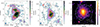 |
Fig. 3. Left: Low-resolution source-subtracted LOFAR image of A773 at 144 MHz overlaid with LOFAR 2σ contours. Middle: Low-resolution source-subtracted uGMRT image of A773 at 650 MHz overlaid with uGMRT 2σ contours. Right: XMM image of A773 overlaid with LOFAR source-subtracted contours. The contour levels are spaced as ( − 2, 2, 4, 8, 16, 32) × σrms. LOFAR and uGMRT source-subtracted images have a resolution of 50′′ × 50′′. The region drawn around the halo represents the r500 scale of the cluster. |
 |
Fig. 4. Same as Fig. 3 but for A1351. The LOFAR and uGMRT source-subtracted images have a resolution of 33′′ × 33′′. |
2.4. Flux density and spectral index measurement
To measure the flux density of the RH in LOFAR and uGMRT images, we adopted two methods, which are explained in the next section.
2.4.1. 2σ contours
In the first method, we integrated the flux density within the region defined by the 2σ contours of the RH. To assess consistency and potential differences in the emission size between LOFAR and uGMRT, we used two regions: one defined by the LOFAR 2σ contours and the other by the uGMRT 2σ contours. For each of these regions, we measured the integrated flux density in both the LOFAR and uGMRT images and derived the corresponding spectral slope. The uncertainty in the flux density was calculated using the following formula,
 (1)
(1)
where f represents the systematic uncertainties due to absolute flux scale errors (see Sects. 2.1 and 2.2). The σrms is the map noise level, Nbeam is the number of beams covering the halo region, and σsub is the uncertainty of the source subtraction in the uv plane, which was calculated by following the procedure described in Botteon et al. (2022). The flux density values are listed in the Table 3.
Flux density and spectral index values for clusters A773 and A1351.
From the measured flux densities, we determined the spectral index (α) and its error. The error in the α was determined as
 (2)
(2)
2.4.2. LOFAR model injection
Injection of an exponential model has been the most widely employed technique to estimate upper limits in cases of RH non-detection, often caused by missing short baselines or poor sensitivity (Brunetti et al. 2007; Venturi et al. 2008; Kale et al. 2013; Bruno et al. 2023). As a step forward to this approach, we adopted a method with the key improvement of using a realistic model: using LOFAR model obtained during the LOFAR imaging process, rather than an idealized exponential profile to inject into the uGMRT visibilities. A similar strategy was employed by Giacintucci et al. (2014), who injected the CLEAN components of a mini-halo observed with the GMRT at 617 MHz into VLA data at 4.86 GHz and 8.44 GHz for different spectral indices. This method not only provides robust upper limits but also allows us to quantify the flux density loss attributed to instrumental limitations. It offer us a more realistic estimate of the halo flux and the spectral index and an opportunity to check for possible systematics in the spectral index estimate. The following steps briefly describe the injection method:
We began the analysis by assuming a flux density to be injected into the uGMRT visibilities. We then rescaled the LOFAR model image to this flux density by adopting the spectral index (α) required to reproduce the corresponding value at 650 MHz. The rescaling was applied to the CLEAN components associated with the RH in the LOFAR low-resolution model, using an inner uv cut of 80λ to include all recoverable diffuse emission by LOFAR. The offset to inject the RH is chosen to be close enough to the center to avoid significant primary beam attenuation, while ensuring that the region is free of contaminating sources or imaging artifacts (see Fig. B.1). After the injection, the “updated” uGMRT dataset is imaged following the standard procedure (see Sects. 2.2 and 2.3), and the recovered flux density of the injected halo is measured within the 2σ contour of the new image. To account for local noise fluctuations and and potential contributions from discrete sources, the flux density measured in the same region prior to injection is subtracted from the recovered flux. If the recovered flux density lies within ±5% of the flux density measured in the observations within 2σ contours, the corresponding injected flux density is considered a reliable estimate of the halo’s flux density. Consequently, the spectral index (α) used to obtain this injected flux is regarded as the reliable spectral index of the halo. This value should be considered a lower limit on α, as it assumes no flux density loss in LOFAR. Bruno et al. (2023, see their Fig. 14) show that flux density losses in LOFAR observations are ≤10% for RHs with diameters between 7.5′ and 10.5′. However, over the broad frequency range of 144–650 MHz, such flux density losses have a negligible impact on the spectral index (α). Since the halos considered in this study have maximum sizes of ∼10′, LOFAR flux density losses are expected to be minimal, and the model images are deemed suitable for injection. The procedure is then repeated iteratively using different values of injection fluxes until the recovered flux matches the observed flux.
If the spectral slope derived from observations between the LOFAR and uGMRT images is steeper than the slope obtained by the injection method, it indicates that the uGMRT has suffered losses due to missing baselines and sensitivity issues.
3. Results
High-resolution LOFAR and uGMRT images of A773 are reported in Fig. 1. The central regions of the cluster show the presence of multiple radio sources. At the resolution of 10′′, the RH detected in LOFAR is larger in size than uGMRT (Fig. 1, left panel).
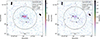 |
Fig. 1. Left: High-resolution LOFAR image of A773 at 144 MHz. Right: High-resolution uGMRT image of A773 at 650 MHz. Both images have resolutions of 10′′ × 10′′, with M500 in units of 1014 M⊙ and rms in mJy/beam. The drawn region represents the r500 scale of the cluster. |
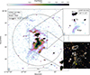 |
Fig. 2. High-resolution LOFAR image of A1351 at 144 MHz with a resolution of 8.64′′ × 4.32′′ and an rms noise of 68 μJy beam−1. The black circle represents the r500 scale of the cluster. Top inset: Zoomed-in view of the cluster center at uGMRT 650 MHz at a resolution of 4.68′′ × 3.34′′. The rms of the uGMRT image is 13 μJy beam−1. Bottom inset: Optical Pan-STARRS (g, r, i) image of the cluster center overlaid with uGMRT radio contours at levels of (9, 18, 27, 36, 45, 52) × σrms. M500 is given in units of 1014 M⊙. |
High-resolution images of A1351 (see Fig. 2) show a more complex radio morphology that include different sources, including one of the two brightest cluster galaxies (BCGs), a tailed galaxy (TG), and an extended region of diffuse emission referred to as the “ridge” (Fig. 2). In the LOFAR high-resolution image, we reached a resolution of 8.64′′ × 4.32′′. However, at this resolution, TG and the ridge are still not resolved. The improved sensitivity and high angular resolution of the uGMRT image (4.68′′ × 3.34′′), clearly reveals both the TG and the ridge structure. Notably, the morphological details of the ridge are distinctly resolved. The ridge extends for a projected length of ∼470 kpc and is located at a projected distance of ∼500 kpc from the center of the cluster. The cluster center was set at the location of the BCG, as described in Barrena et al. (2014). From the head of the TG, the center of the ridge is ∼330 kpc away.
3.1. Radio halo
3.1.1. A773
The RH in A773 is bright and extended, clearly detected in both LOFAR and uGMRT images, and it is located at the center of the cluster, following the X-ray emission (Fig. 3). The halo extends over a largest linear size (LLS) of ∼2 Mpc and is elongated along NE-SW direction in both LOFAR and uGMRT images aligning with the previous studies (Govoni et al. 2001b; Barrena et al. 2007). The integrated flux density values of the halo in LOFAR and uGMRT, based on the LOFAR 2σ contour region, are 143.4 ± 14.5 mJy and 27.1 ± 1.5 mJy, respectively. When measured using the uGMRT 2σ contour regions, the integrated flux density values are 141.1 ± 14.3 mJy and 26.5 ± 1.5 mJy in LOFAR and uGMRT, respectively. The integrated spectral index (α) obtained in the two cases are consistent −1.10 ± 0.08.
In applying the injection method (see Sect. 2.4.2), the flux density of the injected region measured in LOFAR is 149.2 ± 15.1 mJy. Upon rescaling the model to 650 MHz with an α of −1.1, the flux density obtained was 28.9 mJy. When this rescaled flux was injected into the uGMRT visibilities, a flux density of 25.6 mJy was recovered. This value is consistent within ±5% with the flux density measured within the 2σ contour using both LOFAR and uGMRT methods. Therefore, we can conclude that α ∼ −1.1 is a reliable estimate of the halo spectral index, and that ∼28.9 mJy is a likely value for its flux density at 650 MHz, with uGMRT experiencing a flux density loss of approximately ∼7%. The integrated flux density and spectral index values using different methods are reported in Table 3.
3.1.2. A1351
For A1351, the process of source subtraction was challenging due to the presence of many contaminating sources that needed to be removed to isolate the diffuse RH emission. Since the BCG, TG, and the ridge could still leave some residuals after subtraction they were masked during the subtraction of discrete sources while the other contaminants were removed. The RH in A1351 is large, bright, and extended, and is clearly detected in both LOFAR and uGMRT observations. Its morphology broadly follows the distribution of the X-ray emission (Fig. 4) with diffuse emission extending up to r500. However, the faint emission detected near and beyond r500 in the NE region in both the LOFAR and uGMRT images (regions A & B in Fig. 4) remains of uncertain origin. Higher sensitivity observations are necessary to discriminate the possible contribution of discrete sources or residuals in the images. High-resolution images from LOFAR hint at the presence of a faint radio galaxy causing this emission (region A in Fig. 4), although its location at the outskirts of the cluster raises the possibility that it could also be a relic. This region lacks significant X-ray emission and does not show any optical counterpart in Panoramic Survey Telescope and Rapid Response System (Pan-STARRS; Chambers et al. 2016) observation. Therefore, the size and flux density of the RH were measured excluding this faint emission. The halo has a LLS of ∼2.0 Mpc in both LOFAR and uGMRT. If the faint emission near and beyond r500 is included as part of the halo, the total extend of the diffuse emission increases to ∼2.6 Mpc in both the LOFAR and uGMRT images.
The integrated flux density values of the halo in LOFAR and uGMRT using the different methods outlined in Sect. 2.4.1 are reported in Table 3. In both cases, the integrated spectral index is −0.95 ± 0.07. The flux density contributed only by the ridge to the halo is 95.5 ± 9.5 mJy in LOFAR and 21.7 ± 1.1 mJy in uGMRT. When all the contaminants (BCG, tail, and ridge) are taken into account, the total contribution to the halo flux density increases to 121.4 ± 12.1 mJy and 29.5 ± 1.4 mJy in LOFAR and uGMRT, respectively.
The uGMRT flux density measurement aligns (within 1σ uncertainty) with the flux density reported by Chatterjee et al. (2022), which is 87.2 ± 6.1 mJy (within 3σ contours) using GMRT at 610 MHz. In applying the injection method (see Sect. 2.4.2), the flux density of the injected model measured by LOFAR is 408.6 ± 40.9 mJy. Rescaling the model to 650 MHz with α = −0.95, the flux density obtained was 97.6 mJy. When this rescaled flux density was injected into the uGMRT visibilities, a flux density of 88.0 mJy was recovered. This value is within ±5% of the flux density value measured within the 2σ contour using both LOFAR and uGMRT methods. Therefore, we can argue that α ∼ −0.95 is a reliable measurement for the RH spectral index and 97.6 mJy is a reliable measurement of the flux density of the halo at 650 MHz, with uGMRT experiencing a flux density loss of 4–7%.
3.2. Spectral index map
Spectral index maps between LOFAR 144 MHz and uGMRT 650 MHz source-subtracted images were generated applying a common inner uv cut of 200λ to sample the same spatial scales and masking regions below 3σ threshold. The images were convolved to a common resolution, re-gridded, and aligned. Re-gridding was performed using CASA, while image alignment was carried out using BROADBAND RADIO ASTRONOMY TOOLS (BRATS; Harwood et al. 2020) Image Aligner2. The spectral index map of the aligned images was produced using CASA and does not account for flux density losses in uGMRT identified through the real LOFAR model injection. These losses primarily affect the faint, diffuse emission located in the peripheral regions; however, they are on the order of a few percent, as shown in Sects. 3.1.1 and 3.1.2, and therefore do not significantly impact the spectral analysis.
3.2.1. A773
For A773 the resulting spectral index map reveals a spatial variation of the spectral index with values ranging between −1.4 and −0.6 (Fig. 5). To further illustrate this variation, the spectral index measured within radio beam sized grids in the spectral index map is presented as a histogram (Fig. C.1). In the core of the cluster, the spectral index remains constant around −1.0. In the southeast edge of the map, the region that falls inside the 6σ contour shows spectral flattening, and this is attributed to the source subtraction residuals, which becomes prominent at low resolutions. This region also exhibits high spectral index error values, making the spectral index less reliable than in the other regions (see Fig. 5).
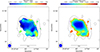 |
Fig. 5. Spectral index map between the source-subtracted images of LOFAR at 144 MHz and uGMRT at 650 MHz of A773 (left panel) and their error map (right panel), with resolutions of 50′′ × 50′′, overlaid with 3 sigma contours of the LOFAR image. The contour levels for LOFAR are set at (3, 6, 9, 12, 27, 41) × σrms, where σrms is 0.30 mJy/beam. |
3.2.2. A1351
For A1351, spectral index maps were generated for both high-resolution and low-resolution radio images. The high-resolution spectral index map (7′′ × 7′′) is important for studying the impact of ridge and other radio features on the halo. To create the high-resolution images, we used a Briggs weighting parameter of −1, with no taper and an inner uv cut of 200λ, for both LOFAR and uGMRT datasets. The spectral index map was then produced following the procedure described earlier (see Fig. 6). From the high-resolution spectral index map, we observe a steepening of the spectral slope along the tail of the TG (Fig. 6). On the other hand, the ridge, does not show any significant spectral gradient; its spectral index is ∼ − 0.9. A previous study by Chatterjee et al. (2022), based on an spectral index map between GMRT and VLA (610 MHz–1.4 GHz), reported a spectral steepening across the ridge, suggesting the presence of a shock downstream. However, in our spectral index map, no clear gradient is detected across the ridge.
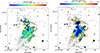 |
Fig. 6. Spectral index map between the high resolution images of LOFAR at 144 MHz and uGMRT at 650 MHz of A1351 (left panel) and its error map (left panel), with resolutions of 7′′ × 7′′. The contour levels for LOFAR are set at (3, 6, 9, 12, 27, 41) × σrms, where σrms is 0.071 mJy/beam. |
For the low-resolution, source-subtracted spectral index map of A1351 (Fig. 7), we adopted a different approach compared to the method used for A773. Specifically, the BCG, TG, and the ridge, were not subtracted before producing the spectral index maps (Fig. 7). The other contaminating sources were removed. This was done intentionally because they are challenging to remove and there could be some residuals of the bright tails even after subtraction. This will also allow us to investigate whether any spectral gradient exists that could suggest a connection to a shock or support the interpretation of the ridge as a radio relic. Spectral flattening is observed in the regions of TG and BCG (Fig. 7), but the image does not provide significant information regarding particle acceleration processes.
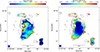 |
Fig. 7. Similar to Fig. 5 but for A1351, with resolutions of 30′′ × 30′′. The contour levels for LOFAR are set at (3, 6, 9, 12, 27, 41) × σrms, where σrms is 0.19 mJy/beam. Note that the BCG, TG, and the ridge were not subtracted in the final source-subtracted LOFAR and uGMRT images used to generate the spectral index map. |
3.3. Point-to-point analysis
To investigate the connection between the thermal and nonthermal components in these galaxy clusters, we performed a point-to-point analysis of their radio and X-ray surface brightness (IRadio–IX relation; Govoni et al. 2001a). Several studies have conducted point-to-point analysis, revealing that clusters with RHs generally exhibit a positive, sublinear trend between the radio and X-ray brightness indicating narrower thermal and broader nonthermal components distribution (Giacintucci et al. 2005; Cova et al. 2019; Xie et al. 2020; Hoang et al. 2021; Santra et al. 2024; Balboni et al. 2024). In our paper, point-to-point analysis was conducted using the methodology described in Balboni et al. (2024) where surface brightness was extracted from the radio (IR) and X-ray (IX) images by constructing a grid over the regions above the 2σ level. Each box inside the grid has an area equal to the radio beam size, ensuring that the measurements remain independent (see Fig. D.1).
3.3.1. A773
In the analysis of the A773 cluster, the source-subtracted images from LOFAR and uGMRT were convolved to a common resolution of 50′′ × 50′′. Focusing on regions above the 2σ noise level, these images were compared with the X-ray image obtained from XMM-Newton (Zhang et al. 2023). As depicted in Fig. 8, the best-fit relation between radio and X-ray surface brightness yields a slope of 0.81 ± 0.06 for LOFAR-XMM and 0.70 ± 0.06 for uGMRT-XMM. This sublinear correlation aligns with the expectations from the turbulent reacceleration model of RHs (Govoni et al. 2001a; Brunetti & Jones 2014; Balboni et al. 2024). The Pearson correlation coefficient rp is 0.87 for LOFAR-XMM and 0.88 for uGMRT-XMM, with a scatter σ of 0.35 and 0.29 around the best-fit relation (see Table 4).
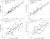 |
Fig. 8. Top: Radio and X-ray surface brightness comparison of LOFAR and uGMRT images at a resolution of 50′′ × 50′′ with an X-ray XMM image of A773 within the regions marked by boxes in Fig. D.1. Bottom: Same but for A1351 at a 33′′ × 33′′ resolution. The red line indicates the best fit, and the dashed blue line is the 2σ contour threshold. The Pearson correlation coefficient is denoted by rp, with the corresponding p-values in brackets. σ indicates the scatter around the best-fit relation. |
Point-to-point analysis of A773 and A1351.
3.3.2. A1351
Similar to cluster A773, the source-subtracted images for cluster A1351 from LOFAR and uGMRT were convolved to a common resolution of 33′′ × 33′′. Regions above the 2σ noise level were compared with the X-ray image obtained from XMM-Newton, and their respective surface brightness within the grids (see Fig. D.1) were plotted (Fig. 8). This analysis yielded a best-fit relation of 0.98 ± 0.15 for LOFAR-XMM, with a Pearson correlation coefficient rp ∼ 0.48 and a scatter σ of 0.87. For uGMRT-XMM, the best-fit relation was 0.93 ± 0.17, with a Pearson correlation coefficient rp ∼ 0.50 and a scatter σ of 0.85 (see Table 4). In both cases, the high value of the scatter might suggest a weak or absent correlation. We decided to investigate which part of the halo contributes more to the scatter, so we divided the RH into two distinct regions: the center and the outer region, fitting them separately. In both regions, the relations were weakly correlated. A further subdivision of the RH into three spatial regions did not improve the correlation. However, this analysis showed that the scatter primarily arises from regions affected by BCG and the ridge. We did not attempt additional subdivisions due to the limited number of grids available for a reliable fit.
4. Discussion
4.1. A773
A773 is a dynamically disturbed cluster characterized by a bimodal velocity distribution of galaxies. Optical observations from Digitized Sky Survey (DSS) reveal two galaxy substructures with one of them aligning with the center of X-ray emission (Govoni et al. 2004). Significant amount of substructure in A773 was first shown by ROSAT (Rizza et al. 1998; Govoni et al. 2001b; Starck & Pierre 1998). A773 has experienced multiple merger events involving one or two massive galaxy groups. One of the major mergers was along the north–south (N–S) direction, involving the cluster and the group that contained the second dominant galaxy in the system. The most recent merger is along NEE-SWW direction, as traced by the X-ray emission (Barrena et al. 2007). Since the X-ray peaks do not correlate with the spatial distribution of galaxies it indicates an advanced merging phase (Barrena et al. 2007). This was further supported by the position of the dominant galaxies along the N-S direction, while the X-ray emission extending along NEE-SWW direction. Barrena et al. (2007) also expect that the merger axis is close to the line of sight (LOS).
From the source-subtracted images of A773, it is evident that the extent of the diffuse radio emission observed in LOFAR and uGMRT is similar (Fig. 3). Contrary to the findings of Govoni et al. (2004), the RH follows the X-ray emission along NEE-SWW direction. The discrepancy may have resulted from the limited sensitivity of the previous radio and X-ray observations. The RH exhibits an integrated spectral index of  . The spectral index map (Fig. 5) and the corresponding histogram (Fig. C.1) reveal significant spatial variations in α, suggesting the presence of complex particle acceleration processes within the cluster.
The point-to-point analysis reveals a best-fit sublinear correlation between the radio and X-ray surface brightness distributions in both LOFAR-XMM and uGMRT-XMM dataset (Fig. 8). There is some scatter present in both plots. The level of scatter is negligible and agrees with the average intrinsic scatter reported by Balboni et al. (2024), who investigated the radio–X-ray correlations in five other clusters hosting RHs. The best-fit relation for LOFAR–XMM is steeper than that for uGMRT–XMM. This difference is likely driven by the flattening of the spectral indices (see Fig. 5) toward the halo outskirts, where the X-ray emission becomes fainter. A possible explanation for the spectral flattening is the presence of particles reaccelerated by merger-driven shocks, likely associated with the recent merger activity along the NE–SW axis. However, we cannot exclude the possibility that additional mechanisms are at work in the cluster.
4.2. A1351
A1351 is also a dynamically disturbed galaxy cluster exhibiting a bimodal velocity distribution with two distinct peaks separated by approximately 2500 km s−1 in the rest frame, indicative of an active merger (Barrena et al. 2014) along the LOS. The X-ray peak coincides with one of the two BCGs, which is also the only one detected in radio (marked as BCG in Fig. 2). Analysis of Chandra X-ray data reveals four substructures along the N–S axis, two of which are associated with the BCGs and are primarily responsible for the observed bimodality in the galaxy velocity distribution. A1351 hosts a giant RH that extends along NE-SW with a LLS of ∼2 Mpc in both LOFAR and uGMRT images (Fig. 4) and the X-ray surface brightness distribution is elongated along N-NE to S-SW axis. The halo is asymmetrical with respect to X-ray emission, consistent with previous studies (Giacintucci et al. 2009; Giovannini et al. 2009; Chatterjee et al. 2022; Botteon et al. 2022). The presence of numerous discrete radio sources at the cluster center complicates the analysis of the RH, as it significantly hinders accurate source subtraction and the study of the diffuse emission. An important feature within this galaxy cluster is the ridge; see Fig. 2. The ridge is claimed to be a radio relic in earlier research of Chatterjee et al. (2022), Giacintucci et al. (2009) and Barrena et al. (2014); but high-sensitivity and high-resolution imaging with uGMRT at 650 MHz (Fig. 2) suggests an atypical morphology. Analysis of Chandra X-ray data by Chatterjee et al. (2022) revealed a surface brightness discontinuity and a temperature jump, indicating a shock propagating along the SW direction. The shock Mach number derived from radio observations and the temperature jump was found to be ≥1.5. It was proposed that since the cluster merger is along the NNE-SSW axis, an axial shock could form the relic (Chatterjee et al. 2022). According to Barrena et al. (2014), since the ridge is situated at the external boundary of the southernmost X-ray clumps, it suggests that it could be a relic associated with a minor merger along the N-S direction. Despite previous X-ray studies favoring the interpretation of the relic, our analysis raises questions about this classification. The ridge’s morphology (Fig. 2), lack of a spectral gradient (Figs. 6), and the presence of an optical counterpart in its central region (Figs. 2) suggest that it is most likely a radio galaxy rather than a projected relic. Furthermore, the tail of the TG interacts with the head of the ridge, supplying relativistic electrons to the ridge and also to the surrounding turbulent medium, where they can be reaccelerated along with electrons from other radio sources within the cluster.
Another unique radio feature observed in A1351 is the extended emission near r500 (Fig. 4, marked as region A). This region was excluded from the calculations of the size and flux density of the RH because of uncertain origin. This region lacks any optical or X-ray counterparts. In their analysis based on VLA data, Giacintucci et al. (2009, refer to their Fig. 2) suggested the possibility of a small radio filament close to the extended emission observed near r500. Instead, it could potentially be associated with a radio galaxy or a relic. This is further supported by the findings of Barrena et al. (2014), who dismissed the filament hypothesis due to the absence of X-ray emission or an optical subcluster in that region. Additionally, the uGMRT image at low resolutions (Fig. 4, region marked B) shows a morphology that deviates from the LOFAR detection. Due to the morphological differences, a direct comparison between the LOFAR and uGMRT image was also not feasible.
The ridge contributes approximately one-third of the total flux density measured for the RH in LOFAR and uGMRT. The RH in A1351 has an integrated flat spectral index of  . The low-resolution spectral index map shows no significant spectral index gradient (Fig. 7). Our results differ significantly from those reported by Chatterjee et al. (2022) at higher frequency, who found a steeper integrated index of α = −1.72 ± 0.33 for the halo and α = −1.63 ± 0.33 for the ridge between GMRT 610 MHz and VLA 1.4 GHz. The difference in the spectral index could arise from several factors. Our analysis is based on GMRT wide band data (LOFAR–uGMRT), whereas their study used GMRT narrow band observations (GMRT–VLA), offering improved bandwidth coverage and sensitivity in our case. There are also differences in source subtraction methods, the specific regions selected for flux density and spectral index measurements, and the possibility of spectral steepening at frequencies higher than 600 MHz.
A1351 is a notable cluster as it hosts a giant RH but deviates from the expected sublinear point-to-point correlation. The comparison between LOFAR-XMM and uGMRT-XMM surface brightness shows significant high scatter, which leads to doubts about the existence of a correlation. The observed correlation and scatter is likely influenced by the central contaminants, which are not a part of the halo but might hide a flatter (sublinear) correlation. This raises the possibility that not all the observed diffuse emission is part of the halo; rather, we may be detecting only a fraction of the halo, with the rest of the emission potentially arising from other sources.
For both clusters, the LOFAR model injection technique was employed to determine the flux density loss of the halos in the uGMRT datasets. This approach is a step forward from the conventional method of injecting an exponential model to find the upper limits. This method can determine the upper limits in the absence of a RH or quantify the flux density loss if a RH has been detected by the telescope. For both A773 and A1351, the flux density loss in the uGMRT datasets ranges between 4% and 7%. Assessing flux density loss is crucial, as losses above 20–30% could bias the results, producing a steeper spectral slope or underestimating the flux density. However, in our analysis, the spectral slopes obtained from the two methods agree within a 1σ uncertainty.
Accurate measurements of the spectral slope and radio flux density are essential for understanding the origin of RHs. In the turbulent reacceleration model, α depends on cluster mass, dynamical state of the merging system, and the mass of any accreted group or cluster (Cassano et al. 2023), providing insights into the physical mechanisms driving halo formation.
Both A773 and A1351 are are massive clusters hosting giant RHs with integrated  . A773 shows signs of past mergers, including a recent core passage, while A1351 is undergoing an active merger. These dynamical states likely generate sufficient turbulent energy to power bright halos observable at high frequencies (e.g., 650 MHz). In addition, the presence of numerous radio galaxies around the halos may also supply seed cosmic-ray electrons for turbulent reacceleration (Vazza & Botteon 2024).
5. Conclusion
From our analysis of the RHs in A773 and A1351 based on LOFAR-uGMRT data, we derived the following conclusions:
-
The galaxy clusters A773 and A1351 are massive merging clusters that both host giant RHs. The LLS of the RHs in A773 and A1351 is ∼2 Mpc in both the LOFAR and uGMRT images.
-
Both A773 and A1351 host numerous radio sources within the halo region. Notably, A1351 contains three significant sources that affect the halo emission: the BCG, a TG, and a ridge. The ridge was considered a relic in Chatterjee et al. (2022), Giacintucci et al. (2009), and Barrena et al. (2014). However, our high-sensitivity and high-resolution images from uGMRT at 650 MHz (Fig. 2) raise a question about the nature of this emission as its morphology resembles that of a radio galaxy.
-
The flux densities and spectral indices were derived using two approaches: measuring flux densities within 2σ contours in LOFAR and uGMRT images, and modeling with injection of real LOFAR data. Both methods yield an integrated flat spectral index of ∼ − 1.0 for both clusters.
-
A773 shows a varying spectral index in the spectral index map with no clear trend. A1351 shows no significant spectral gradients in the spectral index map. Additionally, the ridge in A1351 did not display any spectral gradient, which is in contrast with previous studies (Chatterjee et al. 2022).
-
A point-to-point analysis revealed that A773 exhibits a sublinear relation between radio and X-ray surface brightness in both LOFAR and uGMRT data, which is consistent with expectations of the turbulent reacceleration scenario (Brunetti & Jones 2014). In contrast, A1351 exhibits a weak or absent correlation between LOFAR-XMM and uGMRT-XMM, with a high scatter (σ ∼ 0.85 − 0.87) dominating the relationship. We suggest that the presence of numerous contaminants (discrete and diffuse sources embedded within the halo) may obscure the underlying sublinear relation.
Conducting a LOFAR very long-baseline interferometry and polarization analysis on A1351 could provide further insights into the nature of the ridge and accurate source subtraction.
References
- Abell, G., Corwin, H., Jr, & Olowin, R. 1989, ApJS, 70, 1 [NASA ADS] [CrossRef] [Google Scholar]
- Adam, R., Goksu, H., Brown, S., Rudnick, L., & Ferrari, C. 2021, A&A, 648, A60 [NASA ADS] [CrossRef] [EDP Sciences] [Google Scholar]
- Allen, S., Schmidt, R., Fabian, A., & Ebeling, H. 2003, MNRAS, 342, 287 [NASA ADS] [CrossRef] [Google Scholar]
- Astropy Collaboration (Robitaille, T. P., et al.) 2013, A&A, 558, A33 [NASA ADS] [CrossRef] [EDP Sciences] [Google Scholar]
- Balboni, M., Gastaldello, F., Bonafede, A., et al. 2024, A&A, 686, A5 [NASA ADS] [CrossRef] [EDP Sciences] [Google Scholar]
- Barrena, R., Boschin, W., Girardi, M., & Spolaor, M. 2007, A&A, 467, 37 [NASA ADS] [CrossRef] [EDP Sciences] [Google Scholar]
- Barrena, R., Girardi, M., Boschin, W., De Grandi, S., & Rossetti, M. 2014, MNRAS, 442, 2216 [NASA ADS] [CrossRef] [Google Scholar]
- Biava, N., Bonafede, A., Gastaldello, F., et al. 2024, A&A, 686, A82 [NASA ADS] [CrossRef] [EDP Sciences] [Google Scholar]
- Blasi, P., & Colafrancesco, S. 1999, Astropart. Phys., 12, 169 [Google Scholar]
- Böhringer, H., Voges, W., Huchra, J. P., et al. 2000, ApJS, 129, 435 [Google Scholar]
- Bonafede, A., Intema, H. T., Brüggen, M., et al. 2014, MNRAS, 444, L44 [Google Scholar]
- Botteon, A., Shimwell, T. W., Cassano, R., et al. 2022, A&A, 660, A78 [NASA ADS] [CrossRef] [EDP Sciences] [Google Scholar]
- Briggs, D. S. 1995, Am. Astron. Soc. Meeting Abstr., 187, 112.02 [NASA ADS] [Google Scholar]
- Brunetti, G., & Jones, T. W. 2014, IJMPD, 23, 30007 [Google Scholar]
- Brunetti, G., Venturi, T., Dallacasa, D., et al. 2007, ApJ, 670, L5 [Google Scholar]
- Brunetti, G., Giacintucci, S., Cassano, R., et al. 2008, Nature, 455, 944 [Google Scholar]
- Brunetti, G., Zimmer, S., & Zandanel, F. 2017, MNRAS, 472, 1506 [Google Scholar]
- Bruno, L., Rajpurohit, K., Brunetti, G., et al. 2021, A&A, 650, A44 [NASA ADS] [CrossRef] [EDP Sciences] [Google Scholar]
- Bruno, L., Brunetti, G., Botteon, A., et al. 2023, A&A, 672, A41 [NASA ADS] [CrossRef] [EDP Sciences] [Google Scholar]
- Cassano, R. 2010, A&A, 517, A10 [NASA ADS] [CrossRef] [EDP Sciences] [Google Scholar]
- Cassano, R., & Brunetti, G. 2005, MNRAS, 357, 1313 [Google Scholar]
- Cassano, R., Brunetti, G., & Setti, G. 2006, MNRAS, 369, 1577 [Google Scholar]
- Cassano, R., Ettori, S., Giacintucci, S., et al. 2010, ApJ, 721, L82 [Google Scholar]
- Cassano, R., Ettori, S., Brunetti, G., et al. 2013, ApJ, 777, 141 [Google Scholar]
- Cassano, R., Cuciti, V., Brunetti, G., et al. 2023, A&A, 672, A43 [NASA ADS] [CrossRef] [EDP Sciences] [Google Scholar]
- Chambers, K., Magnier, E., Metcalfe, N., et al. 2016, arXiv e-prints [arXiv:1612.05560] [Google Scholar]
- Chandra, P., Ray, A., & Bhatnagar, S. 2004, ApJ, 612, 974 [Google Scholar]
- Chatterjee, S., Rahaman, M., Datta, A., & Raja, R. 2022, ApJ, 164, 83 [Google Scholar]
- Cova, F., Gastaldello, F., Wik, D. R., et al. 2019, A&A, 628, A83 [NASA ADS] [CrossRef] [EDP Sciences] [Google Scholar]
- Dahle, H., Kaiser, N., Irgens, R., Lilje, P., & Maddox, S. 2002, ApJS, 139, 313 [Google Scholar]
- de Gasperin, F., Dijkema, T. J., Drabent, A., et al. 2019, A&A, 622, A5 [NASA ADS] [CrossRef] [EDP Sciences] [Google Scholar]
- Dennison, B. 1980, ApJ, 239, L93 [Google Scholar]
- Di Gennaro, G., van Weeren, R. J., Cassano, R., et al. 2021, A&A, 654, A166 [NASA ADS] [CrossRef] [EDP Sciences] [Google Scholar]
- Dolag, K., & Enßlin, T. A. 2000, A&A, 362, 151 [NASA ADS] [Google Scholar]
- Ebeling, H., Voges, W., Böhringer, H., et al. 1996, MNRAS, 281, 799 [NASA ADS] [CrossRef] [Google Scholar]
- Giacintucci, S., Venturi, T., Brunetti, G., et al. 2005, A&A, 440, 867 [NASA ADS] [CrossRef] [EDP Sciences] [Google Scholar]
- Giacintucci, S., Venturi, T., Cassano, R., Dallacasa, D., & Brunetti, G. 2009, ApJ, 704, L54 [NASA ADS] [CrossRef] [Google Scholar]
- Giacintucci, S., Markevitch, M., Brunetti, G., et al. 2014, ApJ, 795, 73 [Google Scholar]
- Giacintucci, S., Markevitch, M., Cassano, R., et al. 2017, ApJ, 841, 71 [Google Scholar]
- Giovannini, G., Bonafede, A., Feretti, L., et al. 2009, A&A, 507, 1257 [NASA ADS] [CrossRef] [EDP Sciences] [Google Scholar]
- Govoni, F., Enßlin, T. A., Feretti, L., & Giovannini, G. 2001a, A&A, 369, 441 [NASA ADS] [CrossRef] [EDP Sciences] [Google Scholar]
- Govoni, F., Feretti, L., Giovannini, G., et al. 2001b, A&A, 376, 803 [CrossRef] [EDP Sciences] [Google Scholar]
- Govoni, F., Markevitch, M., Vikhlinin, A., et al. 2004, ApJ, 605, 695 [Google Scholar]
- Harris, C. R., Millman, K. J., Van Der Walt, S. J., et al. 2020, Nature, 585, 357 [NASA ADS] [CrossRef] [Google Scholar]
- Harwood, J. J., Vernstrom, T., & Stroe, A. 2020, MNRAS, 491, 803 [Google Scholar]
- Hoang, D. N., Shimwell, T. W., Osinga, E., et al. 2021, MNRAS, 501, 576 [Google Scholar]
- Holhjem, K., Schirmer, M., & Dahle, H. 2009, A&A, 504, 1 [NASA ADS] [CrossRef] [EDP Sciences] [Google Scholar]
- Hunter, J. D. 2007, Comput. Sci. Eng., 9, 90 [NASA ADS] [CrossRef] [Google Scholar]
- Intema, H. T., van der Tol, S., Cotton, W., et al. 2009, SPAM: Source Peeling and Atmospheric Modeling [Google Scholar]
- Joye, W. A., & Mandel, E. 2003, in Astronomical Data Analysis Software and Systems XII, eds. H. E. Payne, R. I. Jedrzejewski, & R. N. Hook, ASP Conf. Ser., 295, 489 [NASA ADS] [Google Scholar]
- Kale, R., Venturi, T., Giacintucci, S., et al. 2013, A&A, 557, A99 [NASA ADS] [CrossRef] [EDP Sciences] [Google Scholar]
- Kale, R., Venturi, T., Giacintucci, S., et al. 2015, A&A, 579, A92 [NASA ADS] [CrossRef] [EDP Sciences] [Google Scholar]
- Markevitch, M., & Vikhlinin, A. 2007, Phys. Rep., 443, 1 [Google Scholar]
- Mohan, N., & Rafferty, D. 2015, PyBDSF: Python Blob Detection and Source Finder (Astrophysics Source Code Library) [Google Scholar]
- Offringa, A. R., & Smirnov, O. M. 2017, MNRAS, 471, 301 [Google Scholar]
- Offringa, A. R., McKinley, B., Hurley-Walker, N., et al. 2014, MNRAS, 444, 606 [Google Scholar]
- Osinga, E., van Weeren, R., Brunetti, G., et al. 2024, A&A, 688, A175 [NASA ADS] [CrossRef] [EDP Sciences] [Google Scholar]
- Ota, N., & Mitsuda, K. 2004, A&A, 428, 757 [NASA ADS] [CrossRef] [EDP Sciences] [Google Scholar]
- Owen, F., Morrison, G., & Voges, W. 1999, in Diffuse Thermal and Relativistic Plasma in Galaxy Clusters, eds. H. Boehringer, L. Feretti, & P. Schuecker, 9 [Google Scholar]
- Pasini, T., De Gasperin, F., Brüggen, M., et al. 2024, A&A, 689, A218 [NASA ADS] [CrossRef] [EDP Sciences] [Google Scholar]
- Planck Collaboration XXVII. 2016, A&A, 594, A27 [NASA ADS] [CrossRef] [EDP Sciences] [Google Scholar]
- Press, W., & Schechter, P. 1974, ApJ, 187, 425 [Google Scholar]
- Price-Whelan, A. M., Sipőcz, B., Günther, H., et al. 2018, ApJ, 156, 123 [CrossRef] [Google Scholar]
- Rizza, E., Burns, J. O., Ledlow, M. J., et al. 1998, MNRAS, 301, 328 [NASA ADS] [CrossRef] [Google Scholar]
- Robitaille, T. P., & Bressert, E. 2012, APLpy: Astronomical Plotting Library in Python (Astrophysics Source Code Library) [Google Scholar]
- Santra, R., Kale, R., Giacintucci, S., et al. 2024, ApJ, 962, 40 [NASA ADS] [CrossRef] [Google Scholar]
- Savini, F., Bonafede, A., Brüggen, M., et al. 2018, MNRAS, 478, 2234 [Google Scholar]
- Shimwell, T. W., Tasse, C., Hardcastle, M. J., et al. 2019, A&A, 622, A1 [NASA ADS] [CrossRef] [EDP Sciences] [Google Scholar]
- Shimwell, T. W., Hardcastle, M. J., Tasse, C., et al. 2022, A&A, 659, A1 [NASA ADS] [CrossRef] [EDP Sciences] [Google Scholar]
- Smirnov, O. M., & Tasse, C. 2015, MNRAS, 449, 2668 [Google Scholar]
- Springel, V., Frenk, C. S., & White, S. D. 2006, Nature, 440, 1137 [NASA ADS] [CrossRef] [Google Scholar]
- Starck, J.-L., & Pierre, M. 1998, A&AS, 128, 397 [NASA ADS] [CrossRef] [EDP Sciences] [Google Scholar]
- Tasse, C. 2014a, arXiv e-prints [arXiv:1410.8706] [Google Scholar]
- Tasse, C. 2014b, A&A, 566, A127 [NASA ADS] [CrossRef] [EDP Sciences] [Google Scholar]
- Tasse, C., Hugo, B., Mirmont, M., et al. 2018, A&A, 611, A87 [NASA ADS] [CrossRef] [EDP Sciences] [Google Scholar]
- Tasse, C., Shimwell, T. W., Hardcastle, M. J., et al. 2021, A&A, 648, A1 [NASA ADS] [CrossRef] [EDP Sciences] [Google Scholar]
- van Haarlem, M., Wise, M. W., Gunst, A., et al. 2013, A&A, 556, A2 [NASA ADS] [CrossRef] [EDP Sciences] [Google Scholar]
- van Weeren, R. J., Williams, W. L., Hardcastle, M. J., et al. 2016, ApJS, 223, 2 [Google Scholar]
- van Weeren, R. J., de Gasperin, F., Akamatsu, H., et al. 2019, Space Sci. Rev., 215, 16 [Google Scholar]
- van Weeren, R. J., Shimwell, T. W., Botteon, A., et al. 2021, A&A, 651, A115 [NASA ADS] [CrossRef] [EDP Sciences] [Google Scholar]
- van Weeren, R., Timmerman, R., Vaidya, V., et al. 2024, A&A, 692, A12 [NASA ADS] [CrossRef] [EDP Sciences] [Google Scholar]
- Vazza, F., & Botteon, A. 2024, Galaxies, 12, 19 [NASA ADS] [CrossRef] [Google Scholar]
- Venturi, T., Giacintucci, S., Brunetti, G., et al. 2007, A&A, 463, 937 [NASA ADS] [CrossRef] [EDP Sciences] [Google Scholar]
- Venturi, T., Giacintucci, S., Dallacasa, D., et al. 2008, A&A, 484, 327 [NASA ADS] [CrossRef] [EDP Sciences] [Google Scholar]
- Wen, Z., & Han, J. 2013, MNRAS, 436, 275 [NASA ADS] [CrossRef] [Google Scholar]
- Wilber, A. G., Brüggen, M., Bonafede, A., et al. 2018, MNRAS, 473, 3536 [Google Scholar]
- Williams, W. L., van Weeren, R. J., Röttgering, H. J., et al. 2016, MNRAS, 460, 2385 [Google Scholar]
- Xie, C., van Weeren, R. J., Lovisari, L., et al. 2020, A&A, 636, A3 [NASA ADS] [CrossRef] [EDP Sciences] [Google Scholar]
- Zhang, X., Simionescu, A., Gastaldello, F., et al. 2023, A&A, 672, A42 [NASA ADS] [CrossRef] [EDP Sciences] [Google Scholar]
Both clusters belong to the sample of PSZ2 clusters detected in the LoTSS-DR2 https://lofar-surveys.org/planckdr2.html.
Appendix A: Acknowledgements
ABon and MBal acknowledges support from the Horizon Europe ERC CoG project BELOVED, GA n. 101169773. FdG and CG acknowledge support from the ERC Consolidator Grant ULU 101086378. SC acknowledges the support from Rhodes University and the National Research Foundation (NRF), South Africa. R.C. and K.S. acknowledges financial support from the INAF grant 2023 “Testing the origin of giant radio halos with joint LOFAR-uGMRT observations" (1.05.23.05.11). Part of The research activities described in this paper were carried out with contribution of the Next Generation EU funds within the National Recovery and Resilience Plan (PNRR), Mission 4 - Education and Research, Component 2 - From Research to Business (M4C2), Investment Line 3.1 - Strengthening and creation of Research Infrastructures, Project IR0000034 – “STILES - Strengthening the Italian Leadership in ELT and SKA". R.K. acknowledges the support of the Department of Atomic Energy, Government of India, under project no. 12-R&D-TFR-5.02-0700. This paper is based on data obtained with the Giant Metrewave Radio Telescope (GMRT). We thank the staff of the GMRT that made these observations possible. GMRT is run by the National Centre for Radio Astrophysics of the Tata Institute of Fundamental Research. The National Radio Astronomy Observatory is a facility of the National Science Foundation operated under cooperative agreement by Associated Universities, Inc. LOFAR (van Haarlem et al. 2013) is the LOw Frequency ARray designed and constructed by ASTRON. It has observing, data processing, and data storage facilities in several countries, which are owned by various parties (each with their own funding sources), and are collectively operated by the ILT foundation under a joint scientific policy. The ILT resources have benefitted from the following recent major funding sources: CNRS-INSU, Observatoire de Paris and Université d’Orléans, France; BMBF, MIWF-NRW, MPG, Germany; Science Foundation Ireland (SFI), Department of Business, Enterprise and Innovation (DBEI), Ireland; NWO, The Netherlands; The Science and Technology Facilities Council, UK; Ministry of Science and Higher Education, Poland; Istituto Nazionale di Astrofisica (INAF), Italy. This research made use of the Dutch national e-infrastructure with support of the SURF Cooperative (e-infra 180169) and the LOFAR e-infra group. The Jülich LOFAR Long Term Archive and the German LOFAR network are both coordinated and operated by the Jülich Supercomputing Centre (JSC), and computing resources on the supercomputer JUWELS at JSC were provided by the Gauss Centre for Supercomputing e.V. (grant CHTB00) through the John von NeumannInstitute for Computing (NIC). This research made use of the University of Hertfordshire high performance computing facility and the LOFAR-UK computing facility located at the University of Hertfordshire and supported by STFC [ST/P000096/1] and Italian LOFAR-IT computing infrastructure supported and operated by INAF, including the resources within the PLEIADI special "LOFAR" project by USC-C of INAF, and by the Physics Department of Turin University (under the agreement with Consorzio Interuniversitario per la Fisica Spaziale) at the C3S Supercomputing Centre, Italy. The PanSTARRS1 Surveys (PS1) and the PS1 public science archive have been made possible through contributions by the Institute for Astronomy, the University of Hawaii, the Pan-STARRS Project Office, the Max-Planck Society and its participating institutes, the Max Planck Institute for Astronomy, Heidelberg and the Max Planck Institute for Extraterrestrial Physics, Garching, The Johns Hopkins University, Durham University, the University of Edinburgh, the Queen’s University Belfast, the Harvard-Smithsonian Center for Astrophysics, the Las Cumbres Observatory Global Telescope Network Incorporated, the National Central University of Taiwan, the Space Telescope Science Institute, the National Aeronautics and Space Administration under Grant No. NNX08AR22G issued through the Planetary Science Division of the NASA Science Mission Directorate, the National Science Foundation Grant No. AST–1238877, the University of Maryland, Eotvos Lorand University (ELTE), the Los Alamos National Laboratory, and the Gordon and Betty Moore Foundation. This work is based on observations obtained with XMM-Newton, an ESA science mission with instruments and contributions directly funded by ESA Member States and NASA. This research has made use of SAOImageDS9, developed by Smithsonian Astrophysical Observatory (Joye & Mandel 2003). This research made use of APLpy, an open-source plotting package for Python (Robitaille & Bressert 2012), Astropy, a community-developed core Python package for Astronomy (Astropy Collaboration 2013; Price-Whelan et al. 2018), Matplotlib (Hunter 2007) and Numpy (Harris et al. 2020).
Appendix B: LOFAR model injection of radio halos
Injection of the real LOFAR model of A773 RH into the uGMRT image at a position offset from the center without any artifacts.
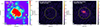 |
Fig. B.1. Real LOFAR model injection into a uGMRT image. Left: LOFAR source-subtracted model image tapered at 100 kpc (144 MHz), with the yellow region indicating the area chosen for injection. Middle: uGMRT source-subtracted image (650 MHz) before injection at the designated RA and Dec. Right: uGMRT source-subtracted image after injection of the LOFAR model rescaled at 650 MHz with α = −1, with the yellow region representing the size of the halo recovered after the injection. |
Appendix C: Distribution of α in the spectral index map
Histogram showing the distribution of spectral index (α) values from the spectral index map in Fig. 5. The α values were averaged within radio beam sized boxes across the map and plotted for regions above the 3σ and 5σ contours.
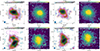 |
Fig. C.1. Distribution of spectral index (α) values in A773, measured within radio-beam-sized boxes (50′′ × 50′′). Blue and red bins represent regions with flux densities above 3σrms and 5σrms, respectively. |
Appendix D: Point-to-point analysis
The region of interest for the point-to-point analysis was divided into boxes with areas equivalent to the beam size, ensuring that the measurements are independent. The radio (Iradio) and X-ray surface brightness (IX) were extracted for these grid cells and subsequently used for the point-to-point correlation analysis (see Fig 8). Shown here are the sampling grids used for A773 and A1351, overlaid on both the LOFAR and uGMRT images.
 |
Fig. D.1. Top-left panels: LOFAR source-subtracted image of A773 at a resolution of 50″×50″ compared with an X-ray XMM image. Top-right panels: uGMRT source-subtracted image of A773 at a resolution of 50″×50″ compared with an X-ray XMM image. Bottom-left panels: LOFAR source-subtracted image of A1351 at a resolution of 33″×33″ compared with an X-ray XMM image. Bottom-right panels: uGMRT source-subtracted image of A1351 at a resolution of 33″×33″ compared with an X-ray XMM image. The boxes indicate the corresponding regions where radio and X-ray brightness were compared, and the circles indicate the masked regions in radio and X-ray images. |
All Tables
All Figures
|
Fig. 3. Left: Low-resolution source-subtracted LOFAR image of A773 at 144 MHz overlaid with LOFAR 2σ contours. Middle: Low-resolution source-subtracted uGMRT image of A773 at 650 MHz overlaid with uGMRT 2σ contours. Right: XMM image of A773 overlaid with LOFAR source-subtracted contours. The contour levels are spaced as ( − 2, 2, 4, 8, 16, 32) × σrms. LOFAR and uGMRT source-subtracted images have a resolution of 50′′ × 50′′. The region drawn around the halo represents the r500 scale of the cluster. |
| In the text | |
|
Fig. 4. Same as Fig. 3 but for A1351. The LOFAR and uGMRT source-subtracted images have a resolution of 33′′ × 33′′. |
| In the text | |
|
Fig. 1. Left: High-resolution LOFAR image of A773 at 144 MHz. Right: High-resolution uGMRT image of A773 at 650 MHz. Both images have resolutions of 10′′ × 10′′, with M500 in units of 1014 M⊙ and rms in mJy/beam. The drawn region represents the r500 scale of the cluster. |
| In the text | |
|
Fig. 2. High-resolution LOFAR image of A1351 at 144 MHz with a resolution of 8.64′′ × 4.32′′ and an rms noise of 68 μJy beam−1. The black circle represents the r500 scale of the cluster. Top inset: Zoomed-in view of the cluster center at uGMRT 650 MHz at a resolution of 4.68′′ × 3.34′′. The rms of the uGMRT image is 13 μJy beam−1. Bottom inset: Optical Pan-STARRS (g, r, i) image of the cluster center overlaid with uGMRT radio contours at levels of (9, 18, 27, 36, 45, 52) × σrms. M500 is given in units of 1014 M⊙. |
| In the text | |
|
Fig. 5. Spectral index map between the source-subtracted images of LOFAR at 144 MHz and uGMRT at 650 MHz of A773 (left panel) and their error map (right panel), with resolutions of 50′′ × 50′′, overlaid with 3 sigma contours of the LOFAR image. The contour levels for LOFAR are set at (3, 6, 9, 12, 27, 41) × σrms, where σrms is 0.30 mJy/beam. |
| In the text | |
|
Fig. 6. Spectral index map between the high resolution images of LOFAR at 144 MHz and uGMRT at 650 MHz of A1351 (left panel) and its error map (left panel), with resolutions of 7′′ × 7′′. The contour levels for LOFAR are set at (3, 6, 9, 12, 27, 41) × σrms, where σrms is 0.071 mJy/beam. |
| In the text | |
|
Fig. 7. Similar to Fig. 5 but for A1351, with resolutions of 30′′ × 30′′. The contour levels for LOFAR are set at (3, 6, 9, 12, 27, 41) × σrms, where σrms is 0.19 mJy/beam. Note that the BCG, TG, and the ridge were not subtracted in the final source-subtracted LOFAR and uGMRT images used to generate the spectral index map. |
| In the text | |
|
Fig. 8. Top: Radio and X-ray surface brightness comparison of LOFAR and uGMRT images at a resolution of 50′′ × 50′′ with an X-ray XMM image of A773 within the regions marked by boxes in Fig. D.1. Bottom: Same but for A1351 at a 33′′ × 33′′ resolution. The red line indicates the best fit, and the dashed blue line is the 2σ contour threshold. The Pearson correlation coefficient is denoted by rp, with the corresponding p-values in brackets. σ indicates the scatter around the best-fit relation. |
| In the text | |
|
Fig. B.1. Real LOFAR model injection into a uGMRT image. Left: LOFAR source-subtracted model image tapered at 100 kpc (144 MHz), with the yellow region indicating the area chosen for injection. Middle: uGMRT source-subtracted image (650 MHz) before injection at the designated RA and Dec. Right: uGMRT source-subtracted image after injection of the LOFAR model rescaled at 650 MHz with α = −1, with the yellow region representing the size of the halo recovered after the injection. |
| In the text | |
|
Fig. C.1. Distribution of spectral index (α) values in A773, measured within radio-beam-sized boxes (50′′ × 50′′). Blue and red bins represent regions with flux densities above 3σrms and 5σrms, respectively. |
| In the text | |
|
Fig. D.1. Top-left panels: LOFAR source-subtracted image of A773 at a resolution of 50″×50″ compared with an X-ray XMM image. Top-right panels: uGMRT source-subtracted image of A773 at a resolution of 50″×50″ compared with an X-ray XMM image. Bottom-left panels: LOFAR source-subtracted image of A1351 at a resolution of 33″×33″ compared with an X-ray XMM image. Bottom-right panels: uGMRT source-subtracted image of A1351 at a resolution of 33″×33″ compared with an X-ray XMM image. The boxes indicate the corresponding regions where radio and X-ray brightness were compared, and the circles indicate the masked regions in radio and X-ray images. |
| In the text | |
Current usage metrics show cumulative count of Article Views (full-text article views including HTML views, PDF and ePub downloads, according to the available data) and Abstracts Views on Vision4Press platform.
Data correspond to usage on the plateform after 2015. The current usage metrics is available 48-96 hours after online publication and is updated daily on week days.
Initial download of the metrics may take a while.