| Issue |
A&A
Volume 707, March 2026
|
|
|---|---|---|
| Article Number | A249 | |
| Number of page(s) | 23 | |
| Section | Stellar atmospheres | |
| DOI | https://doi.org/10.1051/0004-6361/202558001 | |
| Published online | 23 March 2026 | |
A statistical framework for the quantitative spectroscopy of luminous blue stars
Universität Innsbruck, Institut für Astro- und Teilchenphysik,
Technikerstr. 25/8,
6020
Innsbruck,
Austria
★ Corresponding author: This email address is being protected from spambots. You need JavaScript enabled to view it.
Received:
6
November
2025
Accepted:
28
December
2025
Abstract
Context. Quantitative spectroscopy of luminous blue stars relies on detailed non-local thermodynamic equilibrium (non-LTE) model atmospheres whose increasing physical realism makes direct iterative analyses computationally demanding.
Aims. We introduce Machine-learning assisted Uncertainty inference (MAUI), a statistical framework designed for an efficient Bayesian inference of stellar parameters using emulator-based spectral models.
Methods. MAUI employs Gaussian-process-based emulators trained on a limited set of non-LTE simulations, combined with Markov chain Monte Carlo sampling to explore posterior distributions. We validate the approach with recovery experiments and demonstrate it on Galactic late-type O dwarf and early-type B dwarf and subgiant stars.
Results. The emulator reproduces the predictions of full atmosphere models within the quoted uncertainties while reducing computational cost by several orders of magnitude. Posterior distributions are well calibrated with a conservative coverage across all stellar parameters.
Conclusions. The emulator-driven Bayesian inference retains the accuracy of classical analyses at a fraction of the computational expense, which enables posterior sampling that would be prohibitive with direct model evaluations. This positions emulators as a practical tool for high-fidelity spectroscopy of massive stars as atmosphere models grow more demanding.
Key words: methods: statistical / techniques: spectroscopic / stars: atmospheres / stars: early-type / stars: fundamental parameters
© The Authors 2026
 Open Access article, published by EDP Sciences, under the terms of the Creative Commons Attribution License (https://creativecommons.org/licenses/by/4.0), which permits unrestricted use, distribution, and reproduction in any medium, provided the original work is properly cited.
This article is published in open access under the Subscribe to Open model. This email address is being protected from spambots. You need JavaScript enabled to view it. to support open access publication.
1 Introduction
The quantitative spectroscopy of massive stars is central to determining their fundamental parameters, surface abundances, and wind properties. These are essential ingredients for understanding their structure, evolution, and feedback (e.g. Maeder & Meynet 2000; Evans et al. 2006; Crowther 2007; Puls et al. 2008; Langer 2012). OB-type stars with their extended atmospheres and radiatively driven winds (Kudritzki & Puls 2000), require sophisticated non-local thermodynamic equilibrium (non-LTE) radiative transfer and line-formation codes to reproduce the observed spectra (e.g. Hillier & Miller 1998; Pauldrach et al. 2001; Hamann & Gräfener 2004; Puls et al. 2005). The computational expense of these models, however, limits their use in iterative fitting procedures and in studies requiring dense sampling of highly dimensional parameter spaces.
Optimisation techniques based on metaheuristics (Blum & Roli 2003; Talbi 2009) have been successfully applied to the spectroscopic analysis of massive stars (e.g. genetic algorithm, Mokiem et al. 2005). These methods are attractive for their robustness in exploring complex parameter spaces without needing gradients. While metaheuristics are effective at locating global optima, they do not provide a natural means to characterise the underlying posterior distributions, however (Robert & Casella 2004; Posselt & Bishop 2012; Schaer et al. 2018). As a result, uncertainty estimates are typically adopted from fixed criteria (e.g. Brands et al. 2022) and are not derived from the full statistical structure of the inference problem. This remains a concern given the increasing number of free parameters required to model the complex atmospheres of these objects (e.g. Puls et al. 2020) and our incomplete understanding of degeneracies within the associated parameter space.
Bayesian inference frameworks offer a rigorous alternative by exploring posterior probability distributions conditioned on the data (Ford 2005; Gregory 2005). Their drawback is the prohibitive number of model evaluations required. Analogous challenges in climate science and cosmology have been addressed with statistical emulators (machine-learning surrogates trained on a limited set of expensive simulations) that deliver fast predictions with calibrated uncertainties (e.g. Heitmann et al. 2009; Rogers et al. 2019; Watson-Parris et al. 2022).
We present Machine-learning assisted Uncertainty inference (MAUI), a modular framework that builds a statistical emulator with supervised machine-learning techniques. Together with Markov chain Monte Carlo sampling (MCMC), it enables a robust and efficient spectroscopic inference for massive stars. While emulators have been used in other areas of astrophysics (e.g. cosmology, stellar population synthesis, and supernova modelling), applications to quantitative stellar spectroscopy remain limited. MAUI is, to our knowledge, the first Gaussian-process based framework tailored to the high-dimensional non-LTE parameter spaces of hot stars and the first to integrate the emulator directly into a Bayesian workflow. This delivers posterior distributions with full uncertainty quantification at a fraction of the cost of traditional analyses.
This paper is organised as follows. After introducing the methods (Sect. 2), we validate the framework against direct model evaluations (Sect. 3) and apply it to a set of benchmark stars (Sect. 4). This shows that it recovers stellar and wind parameters with high fidelity. Finally, we conclude by discussing future extensions (Sect. 5).
2 Methods
MAUI is not a replacement for stellar atmosphere modelling, but a statistical framework that emulates and accelerates the inference process while fully preserving the physical content of the underlying models. The framework combines synthetic spectra computed with an atmosphere code with statistical components for dimensionality reduction and Gaussian-process emulation, together with Bayesian inference for parameter estimation and uncertainty quantification. The following subsections describe the construction of the training grid, the compression of the stellar spectra and emulator training, and the likelihood formulation used in the Bayesian analysis.
2.1 Model atmosphere and spectral synthesis
For the applications presented in this work, we employ the non-LTE model atmosphere and spectral synthesis code FASTWIND (version 10), originally introduced by Santolaya-Rey et al. (1997), and subsequently extended by Puls et al. (2005), and Rivero González et al. (2011). A detailed account of the current version of the code, including comparisons with alternative codes, is provided by Carneiro et al. (2016). FASTWIND solves the radiative transfer problem for spherically symmetric, expanding stellar atmospheres, under the assumptions of stationary outflow and chemical homogeneity. The code simultaneously ensures statistical equilibrium and energy conservation, treating line-blocking and line-blanketing effects in a consistent, well-tested approximate way, thus reducing the computational effort by more than a factor of 10–20 compared to an exact treatment. The density structure is computed by assuming hydrostatic equilibrium in the deep photosphere and applying the equation of continuity in the wind domain, where the velocity field follows a standard β-type law. A continuous transition between the quasi-hydrostatic photosphere and the accelerating wind is imposed.
FASTWIND allows for parameterised treatments of wind inhomogeneities and X-ray emission from embedded shocks. In the standard microclumping approach, clumps are assumed optically thin, while macroclumping relaxes this assumption and reduces effective opacities in lines and continua (e.g. Hillier 1991; Hamann & Koesterke 1998; Puls et al. 2006; Oskinova et al. 2007; Sundqvist et al. 2010). We neglect any kind of wind inhomogeneities: optical spectra provide limited leverage on clumping (Hα – and HeII 4686 in O-stars – being the only sensitive lines), and our results should thus be interpreted as smooth-wind models, with the usual systematic uncertainties in absolute mass-loss rates. Similarly, while FASTWIND can account for X-ray/EUV emission from wind-embedded shocks (Carneiro et al. 2016; Puls et al. 2020), such effects are negligible for the photospheric lines analysed in this work.
Microturbulence enters the modelling at two distinct stages: first, in the construction of the stellar atmosphere (stratification and level populations), and second, in the computation of the formal solution (emergent spectrum). For the atmosphere calculations we adopt a fixed value of 10 km s−1 for the additional broadening of the line-profiles, though neglecting any turbulent pressure in the hydrostatic/-dynamic description. In the formal solution ξ is treated as a free parameter and allowed to vary from model to model. Although FASTWIND also offers a depth-dependent prescription for ξ in the formal solution, its impact is limited mainly to UV resonance lines formed in the wind and is negligible for the optical photospheric diagnostics considered here. We therefore assume a depth-independent value of ξ in the calculation of the emergent profiles.
Consequently, each FASTWIND simulation is specified by a set of input parameters: effective temperature Teff, effective surface gravity log g, and stellar radius R⋆ (all evaluated at τRoss = 2/3); microturbulent velocity ξ; exponent β of the adopted velocity law; mass-loss rate Ṁ; terminal wind speed v∞; and a set of elemental abundances.
2.2 Model atoms
Atomic data play a central role in non-LTE stellar atmosphere modelling. Modern codes provide a sophisticated numerical framework to solve the radiative transfer and statistical equilibrium equations, but the accuracy of the resulting atmospheric structures and synthetic spectra ultimately depends on the quality and completeness of the underlying atomic data (Przybilla 2010; Hillier 2011). In this sense, non-LTE codes are largely data-driven: the code itself implements the physics and numerical methods, but the computed populations, line strengths, and emergent spectra are only as reliable as the atomic input. Consequently, differences in oscillator strengths, cross-sections, or energy levels can propagate into systematic differences in inferred stellar parameters and abundances.
To achieve high computational efficiency, FASTWIND distinguishes between two classes of elements: so-called explicit and background elements (Puls et al. 2005). Background elements, which are important for the overall atmospheric structure but not used as direct diagnostics, are treated approximately using a fixed atomic database. For the strongest transitions of background elements between carbon and zinc, the radiative transfer is solved in the comoving frame, while the remaining metal lines are treated either by a conventional static radiative transfer in photospheric regions or in the Sobolev approximation. This database (based on Pauldrach et al. 1998) is an integral part of the code distribution and remains unchanged across different applications of FASTWIND.
In contrast, explicit elements (those whose lines are employed as diagnostics in quantitative spectroscopy) are described using detailed, user-supplied atomic data files. These elements are treated with higher precision, including co-moving frame radiative transfer for all relevant transitions. This distinction ensures that spectral features used in fitting procedures are modelled as accurately as possible while retaining overall computational efficiency. Table 1 summarises the model atoms adopted in this study, including the original references where they were first described. The atomic data for H, He, and N II/III/IV are identical to those used in previous FASTWIND studies (Rivero González et al. 2012; Carneiro et al. 2019), ensuring direct continuity with earlier analyses. In contrast, the models for N I, C II, Mg I/II, and Si II–IV are based on newly implemented datasets (see Table 1), while for the O I–III model we use the same data as in our earlier work (Urbaneja et al. 2003, 2005, 2011, 2017). The C III–IV model atoms have been updated in the meantime (J. Puls, priv. comm.).
2.3 Definition of the training simulations
The construction of the training grid is a crucial step, since the extent and sampling of the physical parameter space directly control how accurately the emulator can reproduce model spectra and how broadly it can be applied to real observations. Three main considerations guide the adopted parameter ranges. We describe them individually below.
1. Spectral sensitivity.
The effective parameters explored by the grids are set such that the associated spectral diagnostics remain sensitive across the grid. Because optical wind diagnostics are primarily sensitive to the combination of mass-loss rate, stellar radius, and terminal velocity through the optical-depth invariant Q = Ṁ/( R⋆ v∞)1.5 (Puls et al. 1996), there is no practical gain in treating R⋆ and v∞ as independent free parameters1. Instead, the stellar radius is assigned consistently from the extended flux-weighted gravity–luminosity relation (FGLR) of Kudritzki et al. (2020), which links the flux-weighted gravity log gF = log g − 4 log(Teff/104 K) of an object to its luminosity. The terminal velocity is then specified through a scaling with the escape velocity, v∞ = f (Teff) vesc, adopting the empirical factor f (Teff) from Kudritzki & Puls (2000). This prescription ensures physically motivated values of R⋆ and v∞ while keeping the inference effectively focused on the wind-invariant parameter Q, which instead of Ṁ and v∞ enters the definition of our grids. We note that the actual Ṁ-value that enters the model atmosphere input is calculated from the above equation relating Ṁ with Q, R⋆ and v∞.
The extended FGLR of Kudritzki et al. (2020) is an empirical relation based, for the most part, on detached eclipsing binaries (see the reference for details) and is therefore not tied to a specific set of stellar evolution models. While the calibration sample discussed in the aforementioned work focuses on masses up to ∼20 M⊙, the parameter range relevant for the present study is well bracketed by the systems included in the underlying eclipsing-binary catalogue. Moreover, given the weak sensitivity of optical wind diagnostics to the stellar radius when working with normalised spectra, any residual uncertainty associated with the adopted radius assignment has only a minor impact on the inferred wind-invariant parameter Q.
2. Astrophysical relevance.
The ranges are motivated by the typical properties of the target stars under investigation: they were designed to fully cover the stellar and wind properties expected for the stars analysed in this work. For example, the grid spans micro-turbulent velocities from ξ = 0 to 20 km s−1, encompassing the range typically inferred from metal lines in Galactic OB dwarfs and giants (e.g. Przybilla et al. 2008; Simón-Díaz 2010). Similarly, the wind parameters (β and log Q) were varied across ranges sufficient to reproduce the Hα line morphologies observed in these stars (e.g. Holgado et al. 2018; Carneiro et al. 2019).
3. Computational feasibility.
Rather than employing a fine regular mesh, we use a space-filling sampling strategy to efficiently explore the multidimensional parameter space. Such designs provide good coverage of each parameter range while avoiding redundancy between sampling points.
The training grid consists of 995 FASTWIND simulations, each corresponding to a unique combination of stellar and wind parameters drawn from a maximum-projection Latin-hypercube design (McKay et al. 1979; Stein 1987; Joseph et al. 2015), which ensures uniform coverage of the parameter space without requiring a regular grid.
The stellar parameters covered are the effective temperature Teff, surface gravity log g, microturbulent velocity ξ (formal solution), wind-strength parameter log Q, velocity law exponent β, and individual abundances of He, C, N, O, Mg, and Si. The adopted parameter ranges (Table 2) cover the observational domain of O9–B3 dwarfs and giants, but are extended in some cases beyond typical values. For example, the helium abundance is allowed to reach He/H = 0.07, slightly below the primordial value, not because such low abundances are expected, but to ensure that the emulator samples a sufficiently wide domain of the physical model behaviour. By exposing the emulator to the full range of spectral responses, including regions only marginally relevant for our targets, the statistical model can better learn the underlying dependencies on the physical parameters. This strategy reduces edge effects and leads to more robust interpolations within the astrophysically relevant parameter space, which is where the inference is ultimately performed.
The number of training models was chosen based on the expected smoothness of the spectral response and the dimensionality of the parameter space. The adopted parameter ranges therefore define the applicability domain of the present emulator: its reliability is ensured only within the boundaries of the training grid, and predictions beyond these limits should be regarded as extrapolations and treated with caution.
Model atoms used in the non-LTE calculations.
Parameter ranges adopted for the training grid.
2.4 Dimensionality reduction
A core challenge in emulating stellar spectra lies in their inherently high dimensionality: each synthetic spectrum typically consists of thousands of flux values sampled over a finely spaced wavelength grid. This high dimensionality poses significant computational and statistical challenges for any supervised learning technique, as models must capture complex spectral variations while avoiding overfitting and maintaining efficiency. In particular, regression methods must cope with increased data sparsity and longer training times as the output dimensionality grows. These challenges are especially pronounced in surrogate modelling applications where the goal is to replace computationally expensive simulations with fast emulators trained on a limited number of examples (Bengio et al. 2013; Grover et al. 2018).
To alleviate this problem, we construct an embedding – a lower-dimensional representation of the synthetic spectra – using Principal Component Analysis (PCA, Connolly et al. 1995), whose mathematical foundations are rooted in the Karhunen–Loève Transform (KLT, Loève 1978). Very briefly, the KLT identifies an orthonormal basis that diagonalises the covariance matrix (see below), with eigenvectors capturing the dominant modes of spectral variation. Projecting each spectrum onto this basis yields a set of coefficients, which, along with the eigenvectors, constitutes the lower-dimensional representation of the original space.
In practice, before calculating the embedding, we prepro-cess the synthetic spectra by interpolating them onto a common wavelength grid. The mean2 spectrum,  , is subtracted from all flux vectors to centre the data. The resulting centred data matrix X ∈ ℝN×D, where N is the number of spectra (i.e. models) and D the number of wavelength points, has a sample covariance matrix C ∈ ℝD×D that is defined as

The KLT basis vectors uk are the eigenvectors of C, while the associated eigenvalues λk measure the variance of the training spectra along the corresponding eigenvector directions. In other words, each λk quantifies the amount of variance explained by the corresponding principal component, with larger eigenvalues indicating components that capture more of the structure in the input data.
The matrix of eigenvectors is denoted U = [u1, …, uD ] ∈ ℝD×D, and the corresponding projections

yield the coefficients zik.
Each original spectrum xi can be reconstructed as

where zik is the coefficient of the k-th component for spectrum i.
By retaining only the first K components (those associated with the largest eigenvalues, chosen to explain a given fraction of the total variance) the dimensionality of the output space is reduced from D to K, where K ≪ D. The simulated spectra in the training dataset can then be approximated as

where  denotes the reconstructed approximation of the original spectrum xi. This reconstruction is approximate, as the truncated sum omits the higher-order components; the resulting error corresponds to the residual variance not captured by the first K principal components.
While nonlinear dimensionality reduction methods are increasingly popular in machine learning, we adopt a linear approach for its interpretability. The linear transform ensures that reconstructed spectra remain physically meaningful and avoids spurious artefacts that may arise in nonlinear mappings. Still, linear embeddings, such as those used here, may miss subtle nonlinear dependencies in certain regions of parameter space. Methods like autoencoders or manifold learning (e.g. Hinton & Salakhutdinov 2006; Cunningham & Ghahramani 2015) could, in principle, capture such curved structures more faithfully, though at the cost of reduced interpretability and increased sensitivity to training and hyperparameter choices (Saxe et al. 2019). In this work, we prioritise physical transparency and stability, while leaving nonlinear or hybrid extensions to future developments.
To assess the fidelity of the compact representation independently of the emulator, we use the full training set to compute the reconstruction root-mean-square error (RMSE). Each spectrum in the training grid is projected onto the first K basis vectors to obtain the corresponding coefficients zik, reconstructed, and compared to the original simulation. The RMSE is defined as

where fi is the original i-th spectrum.
The practical impact of this dimensionality reduction is illustrated in Fig. 1, which shows how well spectra can be reconstructed from truncated sets of components. Four cases – K = 4, 11, 30, and 995 (all) – are displayed. A total of K = 45 components are required to keep the global RMSE below 3 × 10⁻³; these account for 99.3% of the total variance in the training set. This threshold is not arbitrary: reconstructions at this level faithfully reproduce the spectral regions most relevant for diagnostics while keeping the dimensionality low enough for an efficient regression. Tests with fewer components led to noticeable degradation in line cores, whereas including more yielded negligible gains at significant computational cost.
The statistical justification for this truncation is summarised in Fig. 2. The left-hand panel shows the eigenvalue spectrum, which exhibits a clear knee near K ≃ 45, beyond which additional components contribute negligibly to the variance. The right-hand panel displays the cumulative explained variance, confirming that the first 45 components capture more than 99% of the variance in the training set. This validates the choice of K adopted for all subsequent analyses.
The wavelength-dependent reconstruction error for K = 45 is shown in Fig. 3. This error, σT(λ), forms part of the total error budget considered during the inference process (see Sect. 2.6). Interestingly, and somewhat counterintuitively, the largest deviation does not occur at Hα, but at the Si IV/O II blend near 4089 Å. Because of its relatively large reconstruction error, this feature is assigned a lower weight in the likelihood evaluation.
2.5 Learning the PC coefficients with Gaussian processes
After compressing each synthetic spectrum into K principal–component (PC) coefficients  , the remaining task is functional interpolation: for any stellar parameter vector θ, we wish to predict the corresponding set of coefficients zk(θ) that would be obtained at that location in parameter space.
For each retained component k, we therefore infer a smooth mapping,

using the spectra in the training set. Once these K mappings are known, the coefficients {zk(θ∗)} for a new parameter vector θ∗ can be predicted, and the corresponding emulated spectrum reconstructed by combining the eigenvectors with these coefficients, exactly as for any original simulation in the grid.
For a given PC, there exists a family of possible functions that could reproduce the corresponding coefficient values from the training grid. Rather than seeking an explicit functional form, our goal is to predict (with quantified uncertainty) the most probable coefficient value for a new parameter vector θ∗. Gaussian-process (GP) regression (Rasmussen & Williams 2006) provides a natural framework for this task, as it defines a probability distribution over functions consistent with the data. Each PC coefficient is modelled independently, which is justified by the orthogonality of the PC basis: the variables are uncorrelated by construction, so modelling them independently preserves information. Although finite grid sampling, truncation to K components, and mild nonlinearities can introduce small residual correlations, these effects are empirically negligible for reconstruction and inference: the off-diagonal elements of the covariance matrix are typically below 2–3% of the total variance, confirming that the assumption of independence is well justified.
The GP prior assumes that the underlying function is smooth and continuous, with continuous derivatives. It is fully specified by a mean function and a covariance kernel, the latter describing how the similarity between two predicted coefficients depends on the distance between their corresponding models in parameter space. The exact form of the covariance kernel and its hyperparameters – typically an amplitude and a set of characteristic length scales (one per model parameter) – determine how rapidly the coefficients are allowed to vary across the grid. The kernel should therefore reflect the expected smoothness of the underlying physical behaviour.
We tested various stationary kernels – whose covariance depends only on separation in parameter space – including squared–exponential, Matérn, and rational-quadratic forms, as well as their linear combinations. The best performance was achieved with a squared-exponential term (capturing smooth global trends) plus a white-noise term (absorbing numerical noise), ensuring accurate, stable interpolation without overfit-ting. In all cases, the noise amplitude is orders of magnitude smaller than the main covariance term.
To account for differing sensitivities of the spectrum to each input parameter, we adopt an automatic-relevance-determination (ARD) kernel (see e.g. Rasmussen & Williams 2006) with a separate length scale per parameter. The hyperparameters are learned from the training data by maximising the marginal likelihood. Before training, both the target coefficients and the input parameters are standardised to zero mean and unit variance to improve numerical conditioning.
The predictive variance of each GP,  , propagates into the emulator uncertainty at each wavelength as
 (1)
(1)
where uk(λ) is the corresponding PC eigenvector. This expression follows directly from the linear reconstruction of the emulated spectrum, assuming the PC coefficients are modelled as independent. The emulator variance contributes directly to the total error budget used in the model–likelihood evaluation (see Sect. 2.6). Unlike the truncation error introduced earlier or the observational noise, this term is model-dependent, i.e. it varies with θ.
Outside the boundaries of the training grid, the GP predictive variances  increase rapidly, leading to a correspondingly large emulator variance
  . This behaviour provides a natural warning against extrapolation and is one of the main reasons we restrict the emulator to the parameter domain covered by the training set.
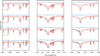 |
Fig. 1 Reconstruction of a representative training spectrum for different truncation levels. Each panel corresponds to a wavelength range and displays the original spectrum (black) together with reconstructions obtained using K = 4, 11, 30, and all principal components (red), vertically offset for clarity. The blue curves show the corresponding residuals (reconstruction original) plotted above each case. The examples illustrate the progressive improvement in the reconstructed line profiles with increasing K. The −selected windows contain strong and weak diagnostic features (H, He, and metals), including the wind–sensitive Hα region. |
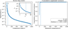 |
Fig. 2 Principal component analysis diagnostics. Left: Scree plot of eigenvalues λk (log scale). The vertical dashed line marks the adopted truncation at K = 45 beyond which the eigenvalues decay rapidly (grey shaded region, inset zoom). Right: Cumulative explained variance, showing that the first 45 components capture over 99% of the total spectral variance. |
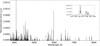 |
Fig. 3 Wavelength-dependent reconstruction error, σK(λ), for the case K = 45. The inset zooms into the region around Hα. |
2.6 Parameter inference
The ultimate goal of quantitative spectroscopy is to determine the atmospheric parameters and surface chemical abundances that characterise an observed spectrum by comparing it with synthetic ones. This process relies on three key ingredients: (1) the observed data, (2) a collection of synthetic spectra, and (3) the metric that quantifies how well a model reproduces the observations. Each of these components directly influences the outcome of the inference. On the observational side, both the quality of the data (e.g. signal-to-noise ratio) and the wavelength coverage determine the available constraints. On the modelling side, the fidelity of the underlying physics and the chosen parameterisation shape the predictive power of the synthetic spectra. Finally, the definition of the distance metric – such as the choice of diagnostic lines and/or the use of weighting schemes – plays a critical role in guiding the inference. A full discussion of these aspects is beyond the scope of the present work, but foreshadowing the results in Sect. 4.4, we stress that they all contribute to the robustness of the derived parameters. As will become apparent in the comparison with literature values, some differences may arise from the characteristics of the observational material or the specific models employed, in addition to methodological choices.
The inference task is naturally formulated within a Bayesian framework, where the aim is to determine the full posterior probability distribution of the parameters, θ, given the data, D. The Bayes theorem provides the formal connection (see e.g. Gregory 2005 for an introduction to Bayesian methods in astronomy)
 (2)
(2)
where ℒ(D | θ) is the likelihood function, quantifying how well a given parameter set reproduces the observed spectrum, π(θ) denotes the prior distribution, and
 (3)
(3)
is the Bayesian evidence (normalisation constant). The evidence ensures that the posterior distribution integrates to unity, but since we are not comparing models with different dimensionalities or physical assumptions, Z plays no role in the present analysis. The inference therefore depends only on the product of likelihood and prior.
The posterior distribution is analytically intractable, and we therefore rely on MCMC sampling to obtain representative draws from it. Specifically, we employ a Metropolis–Hastings algorithm (Metropolis et al. 1953; Hastings 1970), which constructs a Markov chain whose stationary distribution converges to the target posterior. This approach allows us to efficiently explore the probability landscape, quantify uncertainties, and diagnose correlations or degeneracies between parameters (Gregory 2005).
The likelihood is evaluated by comparing the observed spectrum Fobs to the theoretical spectrum (in this case, emulated)  for a trial parameter vector. It takes the form
![Mathematical equation: $ - \ln {\cal L}({\cal D}\mid {\bf{\theta }}) = {1 \over 2}\sum\limits_\lambda {{{\left[ {{{F_\lambda ^{{\rm{obs}}} - {{\hat M}_\lambda }({\bf{\theta }})} \over {{\sigma _\lambda }}}} \right]}^2}} + \ln \left( {2\pi \sigma _\lambda ^2} \right).$](/articles/aa/full_html/2026/03/aa58001-25/aa58001-25-eq17.png) (4)
(4)
The total uncertainty per wavelength point is given by  . Here, σobs represents the observational noise (e.g. photon noise),
  is the predictive variance of the emulator, and σT accounts for the residual wavelength-dependent reconstruction error introduced by truncation of the PCA basis. This formulation assumes that the forward model is unbiased, i.e. that systematic offsets between the simulations and the observations are negligible compared to the stochastic error terms. In practice, such systematics may arise from limitations in the underlying model physics or input data; they are not explicitly modelled here but could, in principle, be represented through an additional “model discrepancy” term σmd in the likelihood.
Future extensions of the framework will incorporate such effects.
Because the emulator is computationally inexpensive to evaluate, it enables extensive MCMC exploration without invoking full radiative transfer calculations at each step. Priors are taken to be uniform within physically motivated ranges, consistent with the limits of the training grid, and we explicitly forbid extrapolation beyond the domain where the emulator is valid. Posterior distributions were sampled using single MCMC chains of 5 × 10⁴ steps, discarding the first half as burn-in. Convergence was assessed using trace plots to verify stationarity and mixing, and by computing the effective sample size (ESS) of each parameter to quantify sampling efficiency. This setup was found to yield stable posterior estimates for all inferred parameters. The inference scheme is applied consistently throughout this work, first to the validation simulations (Sect. 3) and then to the analysis of observed spectra (Sect. 4.4).
2.7 Computational requirements
All components of the emulator and inference pipeline are implemented in IDL 8.8.0 (single-threaded) on Rocky Linux 9.4 (Blue Onyx); we rely on the native IDL linear algebra.
We denote by Nmod the number of models in the training grid, by Npix the wavelength pixels effectively used per spectrum (after masking/rebinning), by Npc the number of retained principal components, and by Nx the number of diagnostic windows used at inference. In practice, increasing Nmod chiefly raises training time; larger Npix mainly affects the initial compression and the cost to reconstruct spectra; and the per-evaluation run-time scales roughly with Nx and the pixels per window because of the instrumental, rotational, and macroturbulent convolutions. Adding more atmospheric parameters typically necessitates a denser grid (larger Nmod) to maintain coverage and often introduces additional spectral variance, which in turn may require a larger Npc to preserve reconstruction fidelity.
During inference, each likelihood evaluation comprises emulator prediction and spectral reconstruction, followed by convolution within Nx diagnostic windows (Nx ≥ 60 here) with the instrumental line–spread function plus rotational and macro-turbulent kernels, resampling to the observed pixels, masking, and the likelihood calculation. The measured mean end-to-end latency per evaluation is teval ≈ 0.8 s.
The one-off cost of generating the training grid can be estimated as follows. A single FASTWIND model takes on average ∼1.0 h of CPU time (with mild variation across parameter space). A ∼1000-model grid therefore represents ~1000 CPU-hours; wall-clock is reduced by parallel runs on multi-core nodes. This cost is paid once and amortised across all targets.
For the grid used here (Nmod = 995, Npix = 90 000, Npc = 45, Nx ≥60), emulator training took ∼9.5 h with a peak memory footprint of 4.5 GB on a dual-socket AMD EPYC 7302 workstation (64 logical CPUs, ∼1.0 TiB RAM). With teval ≈ 0.8 s, a run with 5 × 10⁴ evaluations requires ∼11–12 h of wall-clock on a single thread (linear scaling with evaluation count). For comparison, the same number of direct model evaluations would amount to ∼5 × 10⁴ CPU-hours (computationally intensive for MCMC-scale sampling)3.
3 Validation of the emulator
The purpose of this section is to demonstrate that replacing direct forward simulations with the emulator does not compromise the inference of stellar parameters and abundances. Put differently, we aim to verify that the use of the emulator is effectively equivalent to analysing spectra with the original atmosphere code. To this end, we carried out a series of controlled recovery experiments: synthetic spectra were generated at known parameter values, treated as mock observations, and then analysed with the emulator-based MCMC framework. Comparing the recovered posterior distributions with the true input values allows us to identify potential biases, quantify the reliability of the quoted uncertainties, and assess whether the emulator reproduces the inference process faithfully across the full parameter space.
3.1 Setup
The validation is based on an independent set of 400 FASTWIND simulations that were not used for training. These test points were selected via an independent Latin hypercube design, ensuring broad coverage of the parameter space. The adopted number of simulations represents a compromise between statistical robustness and computational feasibility. Several hundred points are sufficient to obtain stable estimates of reconstruction errors, biases, and coverage fractions across the 11-dimensional parameter space (e.g. McKay et al. 1979; Stein 1987), while avoiding the high cost of much larger validation sets. Smaller test sets (N ≲ 100) proved noticeably noisier in coverage estimates, reflecting the limited statistical stability of ensemble diagnostics in a high-dimensional parameter space rather than inadequate sampling of individual regions of that space. Each test spectrum was treated as a mock observation and analysed using the emulator-based MCMC framework, allowing us to compare the recovered posteriors with the known trueparameter values.
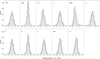 |
Fig. 4 Calibration diagnostics using normal scores of the PIT. The panels show the empirical distributions of z for the difference parameters defining the emulator. The dashed blue curve marks the standard normal (0, 1), with the solid red line providing a kernel density estimate of the results. |
3.2 Metrics
For each parameter θ we computed (i) the mean bias between the recovered posterior mean and the true value, expressed both in physical units (bias) and normalised by the posterior standard deviation (biasz), (ii) the standard deviation of the probit-transformed probability integral transform values (sz), (iii) the root-mean-square error (RMSE) between recovered means and true values in physical units, and (iv) the empirical coverage fractions of the 68% and 95% highest posterior density (HPD) intervals. These quantities jointly assess accuracy (bias, RMSE) and the reliability of the quoted uncertainties (coverage). We note that biasz measures the mean offset between recovered and true values in units of the quoted posterior uncertainty, and therefore provides a dimensionless diagnostic of systematic trends relative to the inferred uncertainty scale, rather than a direct measure of physically significant offsets.
The probability integral transform (PIT) for each parameter and validation spectrum is defined as PIT = Fθ(θtrue), where Fθ is the marginal posterior cumulative distribution function predicted by the emulator and θtrue is the known input value. Under correct specification, PIT values are independent and uniformly distributed on [0, 1]. For visual and quantitative diagnostics we use their normal scores,

where Φ−1 is the inverse of the standard normal cumulative distribution function (CDF), commonly referred to as the probit function. For a well-calibrated predictive model, these normal scores z should follow a standard normal distribution (0, 1) (Gneiting & Raftery 2007; Modrák et al. 2022). In this formulation, an unbiased and properly scaled emulator yields biasz ≈ 0, sz ≈ 1, and empirical coverages close to the nominal 68% and 95% levels.
Figure 4 illustrates the distributions of the normal scores z compared with a standard normal (blue dashed line). The close agreement indicates that the emulator is unbiased and well calibrated, with only modest deviations for a few parameters. Together with the summary statistics in Table 3, this demonstrates that the emulator reproduces the correct posterior distributions within the expected uncertainties.
3.3 Implications
Overall, the validation results show that the emulator performs reliably across all 11 parameters. For photospheric quantities such as Teff and log g, systematic biases are negligible, remaining below ∼10 K and ∼0.01 dex, respectively, while absolute errors are small, with RMSE values of order ∼170 K in Teff and ∼0.02 dex in log g. The chemical abundances of metals, He, and the microturbulent velocity likewise show null biases and low RMSE values (typically below 0.05 dex or their equivalent), with any larger normalised biases reflecting the small inferred posterior uncertainties rather than physically significant offsets. Such small offsets are not expected to produce any noticeable effect on the predicted spectra and thus confirm the accurate recovery of these parameters. The emulator thus provides a faithful and efficient surrogate of the underlying models. We note that the recovery of wind parameters is intrinsically more challenging in the optical, where Hα becomes less sensitive at low mass-loss rates. As a result, both log Q and β tend to show broader, more degenerate posteriors in this regime. This reflects the limitations of the diagnostic rather than shortcomings of the emulator itself.
The outcome of this validation exercise is clear: across the parameter space covered by the training grid, the emulator reproduces the results of the forward simulations within the quoted uncertainties. The posterior distributions obtained with the emulator show consistent coverage, with the 68% intervals tending to be slightly conservative. This implies that the emulator is, if anything, underconfident rather than overconfident in its uncertainty estimates. This conclusion is supported by the scaling factors listed in the last column of Table 3, all of which are smaller than unity, indicating that the quoted errors would need to be reduced to reach perfect calibration. Such mild underconfidence is a desirable feature, as it avoids the risk of underestimated uncertainties and ensures robustness when applied to real data.
Validation statistics for the emulator based on 400 simulations.
4 Analysis of the benchmark stars
The results of the previous section demonstrate that our framework can reliably recover input parameters from synthetic data. We now turn to the crucial step of applying the method to real observations, using well-studied stars as benchmarks to evaluate its performance in practical astrophysical settings. We analyse a sample of Galactic OB-type stars with high-quality spectroscopic data available from public databases, many of which have published atmospheric parameters and abundances based on classical quantitative analyses. The study of such well-characterised stars provides an effective reference set for assessing our method in comparison with literature results. Moreover, the relatively simple atmospheres of OB dwarfs and giants offer an ideal environment to test the reliability of the underlying atomic data, without the additional complications introduced by strong stellar winds or chemical peculiarities.
In the following subsections, we briefly describe the observational data and selected spectral diagnostics, outline the main assumptions of our analysis, present the results of the inference process, and finally compare them with values reported in the literature.
4.1 Observational data
The benchmark sample was designed to span a representative range of late O- and early B-type dwarfs and giants, with low projected rotational velocities to minimise line blending and to enable stringent tests of the adopted model atoms. It comprises 27 Galactic OB stars covering spectral types O9 to B3. Most spectra were retrieved from the IACOB database (Simón-Díaz et al. 2011; Simón-Díaz et al. 2015), complemented by a few additional cases from the Melchiors database (Royer et al. 2024). The observations have high resolving power (R = 25 000–85 000) and signal-to-noise ratios above S/N ~ 200 per pixel, ensuring that all diagnostic lines are well measured. The wavelength coverage extends from 3800–7000 Å, and up to 9200 Å for the data collected with the HERMES spectrograph. Table A.1 summarises the basic stellar and observational information.
For consistency and clarity, we focus primarily on stars previously analysed using classical methods in combination with FASTWIND models, aiming to isolate differences that arise from the inference method rather than from the underlying model-atmosphere code. Minor discrepancies may nonetheless reflect updates in the atomic data, as some of the present model atoms differ from those adopted in earlier studies. To provide a broader basis for future cross-comparisons, we also include a supplementary set of bright, apparently normal OB-type dwarfs and giants that have not been subject to detailed quantitative analysis with FASTWIND. These stars were selected for their high-quality spectra, low projected rotational velocities, and complementary positions in terms of ionisation balance and line-strength regimes. Throughout, we distinguish between the literature comparison sample and the supplementary set, which serves to test the robustness of the method and mitigate potential selection biases.
4.2 Diagnostic spectral features
The optical spectra of OB dwarfs contain a variety of diagnostic lines that allow us to constrain the fundamental parameters and abundances. The diagnostic set includes Balmer lines from Hϵ to Hα, selected He i and He ii transitions (e.g. He i 4471, 4922; He ii 4541, 5411), and representative metal lines from C, N, O, Mg, and Si. A complete list of all transitions considered is provided in Appendix B.1. Together, these lines constitute a well-balanced diagnostic set, covering multiple ionisation stages and a range of line strengths. Combined with the inference algorithm described above and the assumptions outlined in the following section, they form the foundation of our quantitative spectroscopy framework.
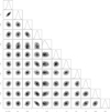 |
Fig. 5 Posterior distributions for HD 36512 (O9.7 V). The results illustrate the typical parameter correlations obtained in our analysis: a clear degeneracy between Teff and log g, and between ξ and the He and metal abundances. Among the latter, the correlation with Si is strongest, reflecting the sensitivity of the Si iii triplet to microturbulence. |
4.3 Fundamental assumptions
Our analysis follows the principle of minimising prior assumptions, ensuring that the observational data provide the primary constraints on the inferred parameters. While fixing certain quantities to expected values can be a pragmatic choice in many studies, such assumptions may also reduce sensitivity to astrophysically relevant inconsistencies. For example, apparent abundance anomalies might arise from spectral contamination from undetected companions, or intrinsic peculiarities of the star. By treating abundances and other parameters as free quantities, we ensure that the inference remains sensitive to such signals, allowing the data to reveal departures from expectation rather than enforcing them a priori.
Our analysis relies on several key assumptions, some of which depart from classical spectroscopic studies. We list them below.
Simultaneous multi-line fitting: All diagnostic lines of H, He, and metals are fitted simultaneously within a single Bayesian framework. This naturally accounts for correlations between parameters without requiring separate two-step determinations.
Microturbulence: a value of ξ is required in the atmosphere calculations, where it can in principle influence the level populations through line opacities and radiative rates, while in the formal solution it acts as an additional Doppler broadening term. In constructing the training grid we adopted a fixed ξ = 10 km s−1 for the model atmosphere, whereas in the inference process ξ is treated as a free parameter shaping the line profiles. A detailed discussion of how microturbulence is constrained in our approach is given in Sect. 4.5.
Wind properties: for low luminosity OB stars, winds are weak. We model the wind-strength parameter Q assuming smooth, unclumped outflows, acknowledging that small clumping effects may be present but are unlikely to significantly affect the optical lines used in this study.
Rotational and macroturbulent broadening: for each star we adopt initial estimates of v sin i and radial–tangential macro-turbulence from the literature, incorporated as Gaussian priors with means and standard deviations reflecting the published values.
Abundances: all elemental abundances are treated as free parameters and constrained simultaneously, rather than adopting expected solar values or fixed ratios.
4.4 Results
Posterior distributions for each star were derived using the Bayesian inference framework outlined in Sect. 2.6. The resulting estimates provide robust stellar and wind parameters with fully quantified uncertainties and covariances. The fundamental parameters are summarised in Table C.1, and the corresponding chemical abundances in Table C.2. Medians and 68% credible intervals are reported throughout. Together, these results provide a complete quantitative description of the benchmark Galactic OB stars analysed in this work.
Figure 5 shows a representative corner plot for HD 36512, illustrating both the marginal posterior distributions and the covariances among parameters. Correlations such as that between microturbulence and abundances, or between Teff and log g, emerge naturally from the joint posterior. This exemplifies a key advantage of the Bayesian framework: parameter degeneracies are explicitly quantified, ensuring that the reported uncertainties reflect the true structure of the solution space.
For the wind parameters, the posteriors of log Q and β show the limited sensitivity of optical diagnostics to weak winds. This behaviour is fully consistent with expectations for late-O and early-B dwarfs and giants with weak winds. In this regime Hα remains predominantly photospheric, with only subtle wind filling in the line core, so the optical diagnostics are mainly sensitive to the overall wind-density scaling encoded in log Q, and carry very little direct information on the detailed shape of the velocity law. As a consequence, the posteriors for β are largely prior-dominated and should be interpreted as reflecting the limited sensitivity of the data. In practice, our results provide robust upper limits and loose constraints on the wind strength, but essentially no meaningful constraint on β for most stars in the sample.
Figures C.1 and C.2 illustrate the overall quality of the results for the O- and B-star subsamples, respectively. The comparisons across broad spectral windows show that the tailored FASTWIND simulations computed using the posterior parameters accurately predict the H, He, and metal lines simultaneously for multiple stars, underscoring the robustness and internal consistency of the Bayesian analysis. Figures C.3 and C.4 present extended spectral ranges for two representative objects, HD 34078 (O9.5 V) and HD 36591 (B1 V). The close agreement across hydrogen, helium, and metal lines demonstrates that the derived parameters provide a consistent description of individual spectra – not only for the diagnostic lines explicitly used in the likelihood, but across the full optical range.
4.4.1 Abundances
A mild decrease in the inferred oxygen abundance with increasing Teff is apparent across the sample (see Fig. 6). The hottest objects tend to show slightly lower abundances than the cooler B-type stars. We interpret this trend as most likely originating from limitations in our current O II model atom at higher ionisation stages rather than as evidence for a genuine depletion of oxygen at higher Teff. An updated O ii model atom incorporating improved atomic data and extended level structure should help to clarify this issue in future analyses. By contrast, neither Mg nor Si shows any significant dependence on Teff or log g. Both elements remain approximately constant within the quoted uncertainties over the full range of stellar parameters sampled.
To assess the absolute abundance scale, we compared the distribution of our inferred elemental abundances with the Cosmic Abundance Standard (CAS) derived for nearby early-type stars by Przybilla et al. (2008) and Nieva & Przybilla (2012). For Mg and Si, the median values in our sample are consistent with the CAS within the 1σ scatter, with a mild systematic difference for Mg (median difference of 0.06 dex). Likewise, the median C abundance shows a shift of 0.12 dex, with our derived values being lower. Nitrogen abundances show a consistent agreement to the CAS baseline, although slightly higher in our case (0.08 dex). Oxygen is on average consistent with the CAS value by ∼0.06 dex, albeit with the aforementioned mild Teff trend discussed above. Overall, the absolute scale of the inferred abundances is compatible with the CAS, and departures from it follow physically interpretable patterns (N enrichment and a possible O offset in the hottest stars) rather than random star-to-star variations. For reference, the Cosmic Abundance Standard itself exhibits a star-to-star dispersion of about 0.05–0.10 dex for C, N, and O. The small differences found here therefore lie well within the intrinsic scatter of the CAS sample and are consistent with normal Galactic abundance variations at solar metallicity.
No systematic trend is found between the derived abundances and the inferred microturbulent velocities, confirming that the adopted treatment of ξ does not introduce spurious correlations in the abundance determinations (see below).
In summary, the abundance patterns inferred by MAUI satisfy two key physical expectations. First, Mg and Si remain approximately constant and do not correlate with Teff or log g, supporting their internal consistency and the high quality of the model atoms. Second, the absolute abundance scale is broadly consistent with CAS values, with a plausible modelling-driven offset in oxygen at the highest Teff. Taken together, these results show that the abundances delivered by the Bayesian multi-line analysis are not only statistically well constrained, but also astrophysically sound.
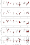 |
Fig. 6 Trends of the derived metal abundances with effective temperature. Each panel shows the inferred abundances of C, N, O, Mg, and Si as a function of Teff for the analysed sample. The error bars correspond to the 68% credible intervals from the posterior distributions. A mild decrease in O abundance toward higher Teff is visible, consistent with the limitations of the current O II model atom at high ionisation stages (see text); no significant trends are found for the other elements. The dash-dotted line marks the CAS value, and the dashed line indicates the median of the derived abundances in each panel. |
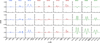 |
Fig. 7 Sensitivity of the selected diagnostic lines to microturbulence, shown as the differential response of the emergent spectrum to changes in ξ. Each row corresponds to a dwarf star of spectral type O9, B0, and B1, respectively. The first seven panels show He I singlet (4387, 4922, 6678 Å) and triplet (4026, 4471, 4713, 5876 Å) lines, followed by the three components of the strong Si III triplet (4553, 4568, 4575 Å). |
4.5 Constraint of the microturbulence
From a spectroscopist’s point of view, microturbulence is a phenomenological parameter introduced to remove systematic trends of derived abundances with line strength, ensuring consistency between weak and strong lines of the same species (e.g. Struve 1929; Struve & Elvey 1934; Gray 2005). Despite its empirical nature, it plays a crucial role in quantitative spectroscopy. Historically, different strategies have been adopted. Some studies derived species-dependent values of ξ (e.g. Trundle et al. 2004; Simón-Díaz 2010; Carneiro et al. 2019), while in the specific case of B-type stars, different authors relied either on O II lines from different multiplets (e.g. Kilian-Montenbruck et al. 1994; Korn et al. 2000), or exclusively on the Si III triplet lines 4553-67-74 (e.g. Kilian 1992; McErlean et al. 1998; Urbaneja et al. 2005, 2011), exploiting its wide range of equivalent widths within a single multiplet to minimise the effect of modelling uncertainties. These approaches have proven effective in practice, though they may yield species-dependent results and make it less straightforward to propagate uncertainties consistently into other parameters. Attempts have also been made to link the spectroscopic ξ to underlying physical processes, most notably sub-surface convection associated with the iron opacity peak (Cantiello et al. 2009). While such works provide valuable insight into a possible origin, the relation between the empirically derived values and the actual velocity fields in stellar atmospheres remains uncertain.
We adopt a complementary strategy in which a single, global ξ is treated as a free parameter in the Bayesian inference, constrained simultaneously by lines of different species and strengths. Figure 7 illustrates the rationale behind this approach. It shows the sensitivity of selected He I lines and of the Si III triplet to changes in ξ, for three representative sets of parameters corresponding to generic O9 (top), B0 (middle), and B1.5 (bottom) dwarfs. Within the Si III triplet, the stronger λ4553 line reacts more strongly than the weaker λ4574 component, with λ4567 showing an intermediate behaviour. This differential sensitivity within a single multiplet is precisely what led to the widespread use of these lines to constrain ξ robustly in B stars. By contrast, in the hotter O9 case the same lines are weak, showing an almost flat response to ξ, largely removing their diagnostic power. In this domain, constraining microturbulence must therefore rely on alternative diagnostics – other ions or line sets – that remain sensitive to ξ. These differences emphasise that the effect of microturbulence depends on the detailed line-formation conditions and on the location of the star in parameter space.
Such behaviour underscores the need for a global treatment of ξ. Because the diagnostic sensitivity varies with spectral types, no single line set remains informative throughout the parameter space. By combining all available diagnostics within a unified Bayesian framework, our method naturally employs the lines that are most sensitive under the local physical conditions, allowing microturbulence to be constrained consistently from the information that is actually available in each regime.
The posterior constraints (Fig. 5) confirm that ξ is well constrained by the combined diagnostics. Both weak and strong lines of individual elements are reproduced simultaneously in our tailored models (Figs. C.1–C.4), providing empirical support for the inferred microturbulent velocities. This agreement across different parts of the curve of growth indicates that the adopted ξ values reconcile abundance determinations from lines of different strengths in a statistically consistent way. By integrating all available diagnostics within a single Bayesian framework, our approach mitigates the biases inherent to line- or species-specific determinations and anchors the inferred microturbulence to the full range of evidence. Finally, we note that ξ is adjusted only in the formal solution, not in the atmospheric structure itself, which may introduce small internal inconsistencies; these are expected to have only minor impact on the present analysis.
Concerning our derived values, a mild systematic behaviour of ξ is apparent within the sample: among the dwarfs, there is a tentative indication that ξ increases slightly with effective temperature, although the effect remains within the formal uncertainties. This tendency is qualitatively consistent with previous findings for OB stars and likely reflect the combined influence of atmospheric extension and thermal structure, but confirmation will require a larger and more homogeneous sample.
4.6 Comparison with previous studies
We compared our results with published FASTWIND based analyses in order to minimise code–dependent systematics and to isolate differences arising from (i) method, (ii) observational material, and (iii) atomic data.
O-type stars. For the late-O stars we used as references the sequence of FASTWIND analyses by Holgado et al. (2018), Carneiro et al. (2019), Martínez-Sebastián et al. (2025), and the most recent work by Holgado et al. (2025). These studies share a common method and provide an internally consistent reference set for assessing our Bayesian inference approach in this hot regime. While all of them deliver fundamental parameters, detailed metal abundances are only provided by Carneiro et al. (2019, , C, N, O) and Martínez-Sebastián et al. (2025, N).
Across the three hottest objects (HD 214680, HD 46202, and HD 34078), our derived effective temperatures and surface gravities agree closely with those of Carneiro et al. (2019), with typical differences well within the combined 1σ uncertainties. Median offsets are of order 70 K in Teff and 0.04 dex in log g, fully consistent with expected variations from diagnostic weighting. HD 36512 shows a larger difference in log g and He abundance. In contrast, the recent analysis by Martínez-Sebastián et al. (2025), which follows the same method as Carneiro et al. (2019), yields parameters consistent with ours, including the N and elevated He abundances. This suggests that the discrepancy with respect to Carneiro et al. (2019) most likely originates from differences in the observational material or its reduction rather than from the inference technique itself.
Microturbulent velocities agree to within ±0.5 km s−1 for all stars in common. Carbon and nitrogen abundances are consistent within uncertainties (mean differences of −0.05 ± 0.10 and +0.03 ± 0.12 dex, respectively), while oxygen is systematically higher in our analysis by ≃ 0.2 dex, consistent with the caution raised by Carneiro et al. (2019) regarding the limitations of their adopted oxygen model atom.
The formal uncertainties in Teff and log g are of the same order as those reported in previous works, reflecting that these parameters are already tightly constrained by well-established diagnostics such as Balmer-line wings and ionisation equilibria. In contrast, the chemical abundances show a clear gain in precision: our formal errors in C and O are smaller by factors of two to five, depending on the star, whereas those in N are comparable or slightly larger. This improvement stems from the global, multi-line nature of the Bayesian inference, which exploits all available spectral information and, by marginalising over all parameters simultaneously, properly accounts for covariances between Teff, log g, ξ, and the elemental abundances. As a result, the derived abundance uncertainties are more realistic and statistically homogeneous across the sample.
To extend the comparison in this regime, we also considered four additional O-type stars (HD 44597, HD 161789, HD 166546, and HD 216898) recently analysed by Holgado et al. (2025), who provide Teff, log g, and He abundances. The effective temperatures agree within 0.3σ for all stars, with a median offset of 0.2σ. Our formal uncertainties are of the same order as those quoted by Holgado et al. (2025). Surface gravities show similarly close agreement, with a median difference of 0.3σ and a maximum of 1.1σ, again accompanied by uncertainties smaller by about a factor of two. Helium abundances are consistent in all four cases. The median ratio of He uncertainties is ~0.6, confirming that our inference yields slightly tighter but statistically compatible constraints.
B-type stars. For the B-type stars we compared our results with stars in the Orion OB1 sample analysed by Simón-Díaz (2010), where Teff is determined from the Si II/III/IV ionisation balance. The sample includes HD 36512, HD 36960, HD 36591, HD 36959, HD 35299, HD 35039, and HD 36430. These objects provide a homogeneous and well-studied reference set for assessing the performance of our Bayesian inference at cooler effective temperatures.
Across the sample, the fundamental parameters show close agreement with the literature. For both Teff and log g, the typical differences correspond to about 0.4 of the combined 1σ uncertainty, with the largest deviations remaining below 1.2σ and 1.8σ, respectively. Our formal 1σ uncertainties are typically 300 K in Teff and 0.05 dex in log g, compared to ~500 K and 0.10 dex in the reference study. This corresponds to uncertainty ratios of roughly 0.6 and 0.5, indicating that our analysis provides constraints of comparable or moderately higher precision for the stellar parameters.
The oxygen and silicon abundances are statistically consistent with those reported by Simón-Díaz (2010). For oxygen, the differences between both studies are typically well within the combined 1σ uncertainties, with an average offset of about half a sigma and the largest case reaching roughly 1.5σ. For silicon, the agreement is even tighter: the average deviation is only about 0.07 dex, and all stars lie within 1σ. The typical uncertainty ratios are about 0.7 for oxygen – our results being approximately 25% more precise – and about 1.1 for silicon, indicating comparable precision overall. These comparisons confirm that the Bayesian multi-line inference yields abundances consistent with the literature while maintaining a uniform statistical treatment across elements.
The microturbulent velocities show somewhat larger star-to-star scatter. On average, the differences correspond to about one to one-and-a-half sigma, reaching up to three sigma in the most discrepant cases, while the typical ratio of formal uncertainties remains close to unity (≈1.2). This suggests that both analyses assign similar formal errors and that the observed differences mainly reflect genuine stellar variations rather than mismatched error estimates. Such scatter is consistent with the known sensitivity of ξ to the details of line formation, and small residual abundance offsets – particularly for oxygen and silicon in this case – are most likely attributable to differences in the underlying atomic data adopted in the respective analyses.
In addition to the main comparison sample, we included τ Sco (HD 149438) as a reference object. This star is the prototypical B0 V standard and has been the subject of numerous detailed spectroscopic analyses (e.g. Mokiem et al. 2005; Simón-Díaz et al. 2006). Its inclusion provides an additional anchor for the early-B regime and allows direct comparison with the extensive literature available for this benchmark. Moreover, τ Sco is a particularly intriguing case, as it is widely accepted (or at least strongly suspected) to be the product of a past stellar merger, which may explain its unusually high helium abundance and complex magnetic field structure. Including this object therefore tests the robustness of our inference scheme for stars with potentially non-standard surface compositions. The agreement of our inferred parameters with those obtained by Mokiem et al. (2005) and Simón-Díaz et al. (2006) is excellent. Unfortunately, none of these two studies determined metal abundances, hence a comparison is not possible.
For the B-type stars our Teff, log g, O, and Si determinations are statistically consistent with the literature, typically within <1σ, and our formal uncertainties are of equal or smaller magnitude. The microturbulent velocities show larger object-to-object deviations at the ∼1–3σ level, consistent with the expected methodological sensitivity of ξ. Overall, the results confirm that the Bayesian inference framework yields parameters and abundances fully compatible with previous analyses, while providing a homogeneous and statistically rigorous treatment across the B-star sample.
Figure 8 presents the comparison for Teff and log g with the literature. O-type stars are shown as squares, with the corresponding reference studies indicated by colour: blue – Carneiro et al. (2019); green – Holgado et al. (2025); pink – Simón-Díaz (2010). The B-type stars are displayed as circles: yellow – Mokiem et al. (2005) (τ Sco); pink – Simón-Díaz (2010).
For both the O- and B-type samples, our results are fully consistent with the stellar parameters and abundances obtained in previous FASTWIND analyses within the quoted uncertainties, while providing smaller and more uniform formal errors. The improvements are most pronounced for log g, Teff, and the CNO abundances. An exception is oxygen in the late-O stars, where our values are systematically higher than those of Carneiro et al. (2019). This difference is understood in light of the simplified oxygen model atom adopted in that study, as noted by the authors themselves. Overall, the remaining residuals are compatible with differences in atomic data or observational material.
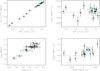 |
Fig. 8 Comparison with literature values. The late O stars are shown as blue squares for Carneiro et al. (2019) and as green diamonds for Holgado et al. (2025). The early/mid B stars are shown as yellow circles Mokiem et al. (2005, τ Sco) and as purple circles for Simón-Díaz (2010). |
5 Discussion
The results presented above establish that MAUI delivers stellar and wind parameters consistent with classical spectroscopic analyses while providing a full probabilistic characterisation of the uncertainties. By accounting for correlations among parameters and propagating uncertainties consistently, MAUI goes beyond line-by-line approaches and offers a transparent quantification of the solution space. A guiding principle of our workflow is to minimise prior assumptions, allowing the observational data to provide the primary constraints: abundances, microturbulence, and other parameters are not fixed to expected values but are derived directly from the spectra. This ensures that potential anomalies are revealed by the analysis rather than masked by assumptions, while recognising that their origin may lie in the stars themselves, in the observations, or in limitations of the models and atomic data.
Although validated here on Galactic late-O and early-B stars, the framework is applicable to other stellar types and model grids. Applications in the literature already include optical spectroscopy of B- and A-type supergiants in the LMC (Urbaneja et al. 2017), near-IR spectroscopy of Galactic Cepheids (Inno et al. 2019), and the large Galactic B-star study by de Burgos et al. (2024). These works confirm that MAUI is robust across spectral types, model-atmosphere codes, and wavelength regimes. A further advantage is computational efficiency: once trained, the emulator enables MCMC-based inference at a fraction of the cost of direct model-atmosphere calculations while retaining rigorous uncertainty propagation. Homogeneous analyses of sizeable samples thus become tractable on standard computing resources.
Beyond the quantitative agreement with previous analyses and the reduction in formal uncertainties, the Bayesian framework also carries an important conceptual implication for how stellar parameters are constrained from spectra.
Classical spectroscopic analyses traditionally associate each stellar parameter with a limited set of diagnostic lines. The effective temperature is derived from ionisation equilibria (for example, Si II/III/IV), the surface gravity from the wings of the Balmer and He I/II lines, and the microturbulent velocity from abundance trends with line strength. This scheme is physically motivated and has long provided robust results, yet it implicitly treats the parameters as quasi-separable quantities, each constrained by an independent subset of observables.
In reality, the spectrum is a global manifestation of the same underlying atmospheric structure. Every wavelength point originates from a complex radiative-transfer calculation that depends on all model parameters – temperature, density, velocity fields, and composition. Consequently, changes in any parameter influence not only its classical diagnostics but also many other spectral features. For instance, metal lines respond to variations in the density distribution and radiation field, thereby carrying indirect information on log g; similarly, the thermal structure and line-blanketing effects couple the strengths of metal and helium lines to Teff. Mathematically, each point of the spectrum can therefore be regarded as sampling the multi-dimensional function Fλ(θ) that encodes the combined physics of the atmosphere, with varying sensitivity to each component of θ.
The Bayesian multi-line inference implemented in MAUI naturally accounts for this coupling. By evaluating the likelihood across wide spectral ranges, the method automatically weighs each wavelength region according to its sensitivity to the parameters, given the model and data quality. Parameters are thus constrained jointly by all available information, without pre-selection of specific diagnostics. The familiar indicators continue to dominate where their sensitivities are strongest, but weaker correlations elsewhere contribute additional information and are reflected in the posterior covariances. This global treatment replaces the approximate separability of the classical approach with a statistically consistent description in which all parameters are inferred simultaneously from the full available information encoded in the spectrum.
The treatment of the microturbulent velocity as a single, global parameter exemplifies this principle: while ξ has no unique diagnostic feature, its value influences the strength and shape of lines from multiple ions. In the Bayesian framework, ξ is therefore constrained by the collective behaviour of all lines rather than by an isolated subset, just as every other parameter is informed by the full spectral information content.
The discussion above highlights that the strength of MAUI lies not only in its quantitative performance but also in its physically consistent, global treatment of the information contained in stellar spectra.
6 Closing remarks
We demonstrated that Gaussian process emulators, combined with a dimensionality reduction and MCMC sampling, provide a rigorous and computationally efficient framework for quantitative spectroscopy of massive stars. The approach yielded transparent uncertainty estimates and propagated parameter covariances consistently while reducing the computational cost by several orders of magnitude compared to direct atmosphere calculations. For the scale of the analyses we presented, the method was fully tractable: A single MCMC run with 5 × 10⁴ steps was completed on standard workstations, which enabled homogeneous studies of moderate-sized samples.
The method is broadly applicable to other stellar types and model grids. Extensions of the training grids, improved treatments of correlated GP components, and refined uncertainty calibration will further enhance the robustness of MAUI for quantitative spectroscopy of hot stars. The current emulator is restricted to optical spectra, for which the wind parameters such as log Q and β remain only weakly constrained. It is essential to incorporate UV and IR diagnostics for a more complete description of stellar outflows.
The MAUI framework is fully code-agnostic and can be coupled to any advanced stellar atmosphere code. Its emulation capability is particularly advantageous for computationally intensive models such as CMFGEN (Hillier & Miller 1998), and first tests have already been successfully conducted. The same strategy will enable systematic comparisons between different atmosphere codes in overlapping parameter regimes and the inclusion of additional physical quantities (e.g. clumping parameters, including the treatment of optically thick clumping (e.g. Hawcroft et al. 2021; Brands et al. 2022)) to investigate their correlations and the effect on the inferred stellar and wind properties.
For very large spectroscopic surveys, neural network emulators will complement MAUI by offering millisecond predictions at the cost of less transparent uncertainty estimates. A hybrid strategy is therefore appealing: GP-based emulators such as MAUI for rigorous uncertainty-aware inference and validation, complemented by deep-learning surrogates for fast exploratory analyses. As stellar atmosphere models evolve toward 3D structures, time dependence, and detailed wind dynamics, their computational demands will continue to grow. Emulator-based inference will thus become increasingly essential, with developments such as adaptive training, sparse or parallelised GPs, and systematic validation under realistic observational conditions to ensure that MAUI remains accurate and robust in diverse spectral regimes.
By enabling robust and homogeneous stellar parameters, the framework directly supports applications ranging from stellar evolution and feedback studies to the interpretation of large spectroscopic surveys. In this context, MAUI provides a practical route towards exploiting the full information content of high-resolution spectra. This bridges the gap between detailed atmosphere modelling and a statistically rigorous inference.
In this way, emulator-based inference transforms quantitative spectroscopy from a labour-intensive art into a scalable uncertainty-aware tool for the next generation of stellar astrophysics.
Acknowledgements
We are grateful to J. Puls for providing careful and insightful comments on the manuscript, which helped to improve its clarity and presentation. We also thank N. Przybilla for generously sharing his excellent model atoms, which were essential for this work. Finally, we thank the referee for a constructive and thoughtful report that helped to clarify several aspects of the paper. The IACOB spectroscopic database is based on observations made with the Nordic Optical Telescope operated by the Nordic Optical Telescope Scientific Association, and the Mercator Telescope , operated by the Flemish Community, both at the Observatorio de El Roque de los Muchachos (La Palma, Spain) of the Instituto de Astrofísica de Canarias.
References
- Becker, S. R., & Butler, K. 1988, A&A, 201, 232 [NASA ADS] [Google Scholar]
- Bengio, Y., Courville, A., & Vincent, P. 2013, IEEE Trans. Pattern Anal. Mach. Intell., 35, 1798 [CrossRef] [Google Scholar]
- Blum, C., & Roli, A. 2003, ACM Comput. Surv., 35, 268 [CrossRef] [Google Scholar]
- Brands, S. A., de Koter, A., Bestenlehner, J. M., et al. 2022, A&A, 663, A36 [Google Scholar]
- Cantiello, M., Langer, N., Brott, I., et al. 2009, A&A, 499, 279 [NASA ADS] [CrossRef] [EDP Sciences] [Google Scholar]
- Carneiro, L. P., Puls, J., Sundqvist, J. O., & Hoffmann, T. L. 2016, A&A, 590, A88 [NASA ADS] [CrossRef] [EDP Sciences] [Google Scholar]
- Carneiro, L. P., Puls, J., & Hoffmann, T. L. 2018, A&A, 615, A4 [Google Scholar]
- Carneiro, L. P., Puls, J., Hoffmann, T. L., Holgado, G., & Simón-Díaz, S. 2019, A&A, 623, A3 [NASA ADS] [CrossRef] [EDP Sciences] [Google Scholar]
- Connolly, A. J., Szalay, A. S., Bershady, M. A., Kinney, A. L., & Calzetti, D. 1995, AJ, 110, 1071 [Google Scholar]
- Crowther, P. A. 2007, ARA&A, 45, 177 [Google Scholar]
- Cunningham, J. P., & Ghahramani, Z. 2015, J. Mach. Learn. Res., 16, 2859 [Google Scholar]
- de Burgos, A., Simón-Díaz, S., Urbaneja, M. A., & Puls, J. 2024, A&A, 687, A228 [NASA ADS] [CrossRef] [EDP Sciences] [Google Scholar]
- Evans, C. J., Lennon, D. J., Smartt, S. J., & Trundle, C. 2006, A&A, 456, 623 [CrossRef] [EDP Sciences] [Google Scholar]
- Ford, E. B. 2005, AJ, 129, 1706 [Google Scholar]
- Gneiting, T., & Raftery, A. E. 2007, J. Roy. Statist. Soc.: Ser. B (Statist. Methodol.), 69, 243 [Google Scholar]
- Gray, D. F. 2005, The Observation and Analysis of Stellar Photospheres, 3rd edn. (Cambridge: Cambridge University Press) [Google Scholar]
- Gregory, P. C. 2005, Bayesian Logical Data Analysis for the Physical Sciences: A Comparative Approach with Mathematica Support (Cambridge University Press) [Google Scholar]
- Grover, A., Zweig, G., & Ermon, S. 2018, in Proceedings of the 35th International Conference on Machine Learning, 80, PMLR, 1837 [Google Scholar]
- Hamann, W. R., & Koesterke, L. 1998, A&A, 335, 1003 [Google Scholar]
- Hamann, W. R., & Gräfener, G. 2004, A&A, 427, 697 [NASA ADS] [CrossRef] [EDP Sciences] [Google Scholar]
- Hastings, W. K. 1970, Biometrika, 57, 97 [Google Scholar]
- Hawcroft, C., Sana, H., Mahy, L., et al. 2021, A&A, 655, A67 [NASA ADS] [CrossRef] [EDP Sciences] [Google Scholar]
- Heitmann, K., Higdon, D., White, M., et al. 2009, ApJ, 705, 156 [Google Scholar]
- Hillier, D. J. 1991, A&A, 247, 455 [NASA ADS] [Google Scholar]
- Hillier, D. J. 2011, Ap & SS, 336, 87 [Google Scholar]
- Hillier, D. J., & Miller, D. L. 1998, ApJ, 496, 407 [NASA ADS] [CrossRef] [Google Scholar]
- Hinton, G. E., & Salakhutdinov, R. R. 2006, Science, 313, 504 [Google Scholar]
- Holgado, G., Simón-Díaz, S., Barbá, R. H., et al. 2018, A&A, 613, A65 [NASA ADS] [CrossRef] [EDP Sciences] [Google Scholar]
- Holgado, G., Simón-Díaz, S., & Herrero, A. 2025, A&A, 703, A 175 [Google Scholar]
- Inno, L., Urbaneja, M. A., Matsunaga, N., et al. 2019, MNRAS, 482, 83 [Google Scholar]
- Jokuthy, A. 2002, PhD thesis, Diploma thesis, University Munich [Google Scholar]
- Joseph, V. R., Gul, E., & Ba, S. 2015, Biometrika, 102, 371 [CrossRef] [MathSciNet] [Google Scholar]
- Kilian, J. 1992, A&A, 262, 171 [Google Scholar]
- Kilian-Montenbruck, J., Gehren, T., & Nissen, P. E. 1994, A&A, 291, 757 [NASA ADS] [Google Scholar]
- Korn, A. J., Becker, S. R., Gummersbach, C. A., & Wolf, B. 2000, A&A, 353, 655 [NASA ADS] [Google Scholar]
- Kudritzki, R.-P., & Puls, J. 2000, ARA&A, 38, 613 [Google Scholar]
- Kudritzki, R.-P., Urbaneja, M. A., & Rix, H.-W. 2020, ApJ, 890, 28 [NASA ADS] [CrossRef] [Google Scholar]
- Langer, N. 2012, ARA&A, 50, 107 [Google Scholar]
- Loève, M. 1978, Graduate Texts in Mathematics, 45, Probability Theory I, 4th edn. (Springer) [Google Scholar]
- Maeder, A., & Meynet, G. 2000, ARA&A, 38, 143 [Google Scholar]
- Martínez-Sebastián, C., Simón-Díaz, S., Jin, H., et al. 2025, A&A, 693, L10 [NASA ADS] [CrossRef] [EDP Sciences] [Google Scholar]
- McErlean, N. D., Lennon, D. J., & Dufton, P. L. 1998, A&A, 329, 613 [NASA ADS] [Google Scholar]
- McKay, M. D., Beckman, R. J., & Conover, W. J. 1979, Technometrics, 21, 239 [Google Scholar]
- Metropolis, N., Rosenbluth, A. W., Rosenbluth, M. N., Teller, A. H., & Teller, E. 1953, J. Chem. Phys., 21, 1087 [Google Scholar]
- Modrák, M., Talts, S., Bürkner, P.-C., Gabry, J., & Vehtari, A. 2022, arXiv e-prints [arXiv:2211.02383] [Google Scholar]
- Mokiem, M. R., de Koter, A., Puls, J., et al. 2005, A&A, 441, 711 [NASA ADS] [CrossRef] [EDP Sciences] [Google Scholar]
- Nieva, M. F., & Przybilla, N. 2008, A&A, 481, 199 [NASA ADS] [CrossRef] [EDP Sciences] [Google Scholar]
- Nieva, M. F., & Przybilla, N. 2012, A&A, 539, A 143 [Google Scholar]
- Oskinova, L. M., Hamann, W. R., & Feldmeier, A. 2007, A&A, 476, 1331 [NASA ADS] [CrossRef] [EDP Sciences] [Google Scholar]
- Pauldrach, A. W. A., Hoffmann, T. L., & Lennon, M. 2001, A&A, 375, 161 [NASA ADS] [CrossRef] [EDP Sciences] [Google Scholar]
- Pauldrach, A. W. A., Lennon, M., Hoffmann, T. L., et al. 1998, in Astronomical Society of the Pacific Conference Series, 131, Properties of Hot Luminous Stars, ed. I. Howarth, 258 [Google Scholar]
- Posselt, D. J., & Bishop, C. H. 2012, Monthly Weather Rev., 140, 1957 [Google Scholar]
- Przybilla, N. 2010, in EAS Publications Series, 43, eds. R. Monier, B. Smalley, G. Wahlgren, & P. Stee, 115 [Google Scholar]
- Przybilla, N., & Butler, K. 2001, A&A, 379, 955 [NASA ADS] [CrossRef] [EDP Sciences] [Google Scholar]
- Przybilla, N., Butler, K., Becker, S. R., Kudritzki, R. P., & Venn, K. A. 2000, A&A, 359, 1085 [NASA ADS] [Google Scholar]
- Przybilla, N., Nieva, M.-F., & Butler, K. 2008, ApJ, 688, L103 [CrossRef] [Google Scholar]
- Puls, J., Kudritzki, R. P., Herrero, A., et al. 1996, A&A, 305, 171 [Google Scholar]
- Puls, J., Urbaneja, M. A., Venero, R., et al. 2005, A&A, 435, 669 [NASA ADS] [CrossRef] [EDP Sciences] [Google Scholar]
- Puls, J., Markova, N., Scuderi, S., et al. 2006, A&A, 454, 625 [NASA ADS] [CrossRef] [EDP Sciences] [Google Scholar]
- Puls, J., Vink, J. S., & Najarro, F. 2008, A&A Rev., 16, 209 [Google Scholar]
- Puls, J., Najarro, F., Sundqvist, J. O., & Sen, K. 2020, A&A, 642, A172 [EDP Sciences] [Google Scholar]
- Rasmussen, C. E., & Williams, C. K. I. 2006, Gaussian Processes for Machine Learning, Adaptive Computation and Machine Learning (MIT Press) [Google Scholar]
- Rivero González, J. G., Puls, J., & Najarro, F. 2011, A&A, 536, A58 [NASA ADS] [CrossRef] [EDP Sciences] [Google Scholar]
- Rivero González, J. G., Puls, J., Massey, P., & Najarro, F. 2012, A&A, 543, A95 [NASA ADS] [CrossRef] [EDP Sciences] [Google Scholar]
- Robert, C. P., & Casella, G. 2004, Monte Carlo Statistical Methods, 2nd edn. (New York: Springer) [Google Scholar]
- Rogers, K. K., Peiris, H. V., Pontzen, A., et al. 2019, J. Cosmol. Astropart. Phys., 2019, 031 [Google Scholar]
- Royer, P., Merle, T., Dsilva, K., et al. 2024, A&A, 681, A107 [NASA ADS] [CrossRef] [EDP Sciences] [Google Scholar]
- Santolaya-Rey, A. E., Puls, J., & Herrero, A. 1997, A&A, 323, 488 [NASA ADS] [Google Scholar]
- Saxe, A. M., Bansal, Y., Dapello, J., et al. 2019, J. Statist. Mech. Theory Exp., 2019, 124020 [Google Scholar]
- Schaer, C., Kühne, R., & Rinke, P. 2018. in Evolutionarv Computation in Combinatorial Optimization (Cham: Springer), 15 [Google Scholar]
- Simón-Díaz, S. 2010, A&A, 510, A22 [NASA ADS] [CrossRef] [EDP Sciences] [Google Scholar]
- Simón-Díaz, S., Castro, N., Garcia, M., Herrero, A., & Markova, N. 2011, Bull. Soc. Roy. Sci. Liege, 80, 514 [Google Scholar]
- Simón-Díaz, S., Herrero, A., Esteban, C., & Najarro, F. 2006, A&A, 448, 351 [NASA ADS] [CrossRef] [EDP Sciences] [Google Scholar]
- Simón-Díaz, S., Negueruela, I., Apellániz, J. M., et al. 2015, arXiv e-prints [arXiv:1504.04257] [Google Scholar]
- Stein, M. 1987, Technometrics, 29, 143 [CrossRef] [MathSciNet] [Google Scholar]
- Struve, O. 1929, ApJ, 69, 173 [Google Scholar]
- Struve, O., & Elvey, C. T. 1934, ApJ, 79, 409 [Google Scholar]
- Sundqvist, J. O., Puls, J., & Feldmeier, A. 2010, A&A, 510, A11 [NASA ADS] [CrossRef] [EDP Sciences] [Google Scholar]
- Talbi, E.-G. 2009, Metaheuristics: From Design to Implementation (Wiley) [Google Scholar]
- Trundle, C., Lennon, D. J., Puls, J., & Dufton, P. L. 2004, A&A, 417, 217 [NASA ADS] [CrossRef] [EDP Sciences] [Google Scholar]
- Urbaneja, M. A. 2004, PhD thesis, Universidad de La Laguna, La Laguna, Spain [Google Scholar]
- Urbaneja, M. A., Herrero, A., Bresolin, F., et al. 2003, ApJ, 584, L73 [Google Scholar]
- Urbaneja, M. A., Herrero, A., Kudritzki, R. P., et al. 2005, ApJ, 635, 311 [NASA ADS] [CrossRef] [Google Scholar]
- Urbaneja, M. A., Herrero, A., Lennon, D. J., Corral, L. J., & Meynet, G. 2011, ApJ, 735, 39 [NASA ADS] [CrossRef] [Google Scholar]
- Urbaneja, M. A., Kudritzki, R. P., Gieren, W., et al. 2017, AJ, 154, 102 [NASA ADS] [CrossRef] [Google Scholar]
- Watson-Parris, D., Rao, Y., Olivié, D., et al. 2022, J. Adv. Model. Earth Syst., 14, e2021MS002954 [Google Scholar]
This statement applies to the parameter space covered in the present work.
Arithmetic mean.
Forward model simulations can be parallelised across cores, reducing wall-clock time (e.g. on our 32–64-way machine, 5 × 10⁴ would still require ∼32–65 runs days). The emulator builds on FASTWIND to enable MCMC-scale posterior sampling; it is intended as a statistical accelerator rather than a replacement for the underlying physical modelling.
Appendix A Benchmark stars
Spectral classification and basic reference information for the reference set of stars.
Appendix B Diagnostic lines
Table B.1 lists the spectral lines included in the likelihood evaluation. These features constitute the set of diagnostics used by MAUI to constrain the stellar and wind parameters and chemical abundances in the Bayesian analysis. The adopted line selection covers the main ionisation equilibria of key elements, together with representative metal lines that are sensitive to microturbulence and abundance variations.
The underlying FASTWIND simulations include a much larger number of transitions, many of which are not explicitly included in the likelihood but are still predicted by the synthetic spectra. Some of these additional lines can be seen in the figures comparing the observed spectra with the model predictions (Figs. C.1–C.4), where they provide a qualitative consistency check on the overall model performance.
Spectral lines included in the likelihood evaluation.
Appendix C Detailed results
This appendix presents the full set of tables and figures containing the results of the Bayesian analysis discussed in Sect. 4.4.
Fundamental parameters of the Galactic OB stars derived from our Bayesian analysis.
Chemical abundances of the Galactic OB stars derived from our Bayesian aalysis.
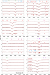 |
Fig. C.1 Representative spectral windows for selected O9-B0 stars. Each panel compares the observed spectra with the tailored FASTWIND models calculated for the final parameters derived from the Bayesian analysis. Multiple stars are shown in each panel (vertically shifted for clarity). The simultaneous agreement across H, He, and metal lines demonstrates the robustness of the inferred parameters for the late O/early B stars. Due to the possible effect of the magnetic field, the Hα core was excluded from the evaluation of the model likelihood for HD 149438. |
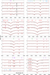 |
Fig. C.2 As Fig. C.1, but for selected B-type stars in the sample. The consistent fits across diagnostic lines of H, He, and metals highlight the reliability of the modelling and the internal consistency of the results for the B-type dwarfs/giants. |
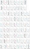 |
Fig. C.3 HD 34078 (O9.5 V): comparison between the observed spectrum (black) and synthetic spectra (coloured) for selected diagnostic lines of H, He, C, N, O, Mg, and Si. The synthetic spectra were computed with FASTWIND using the stellar parameters and abundances obtained from the Bayesian analysis. The good agreement across multiple ions demonstrates the consistency of the inferred parameters and the robustness of the global fitting approach. The horizontal axis is given in pixel number rather than wavelength; the corresponding spectral ranges are indicated by the panel labels. The names identifying the sub-panels are orientative only: each panel may include several spectral features, and the label marks approximately the central wavelength of the region shown. |
All Tables
Spectral classification and basic reference information for the reference set of stars.
Fundamental parameters of the Galactic OB stars derived from our Bayesian analysis.
Chemical abundances of the Galactic OB stars derived from our Bayesian aalysis.
All Figures
|
Fig. 1 Reconstruction of a representative training spectrum for different truncation levels. Each panel corresponds to a wavelength range and displays the original spectrum (black) together with reconstructions obtained using K = 4, 11, 30, and all principal components (red), vertically offset for clarity. The blue curves show the corresponding residuals (reconstruction original) plotted above each case. The examples illustrate the progressive improvement in the reconstructed line profiles with increasing K. The −selected windows contain strong and weak diagnostic features (H, He, and metals), including the wind–sensitive Hα region. |
| In the text | |
|
Fig. 2 Principal component analysis diagnostics. Left: Scree plot of eigenvalues λk (log scale). The vertical dashed line marks the adopted truncation at K = 45 beyond which the eigenvalues decay rapidly (grey shaded region, inset zoom). Right: Cumulative explained variance, showing that the first 45 components capture over 99% of the total spectral variance. |
| In the text | |
|
Fig. 3 Wavelength-dependent reconstruction error, σK(λ), for the case K = 45. The inset zooms into the region around Hα. |
| In the text | |
|
Fig. 4 Calibration diagnostics using normal scores of the PIT. The panels show the empirical distributions of z for the difference parameters defining the emulator. The dashed blue curve marks the standard normal (0, 1), with the solid red line providing a kernel density estimate of the results. |
| In the text | |
|
Fig. 5 Posterior distributions for HD 36512 (O9.7 V). The results illustrate the typical parameter correlations obtained in our analysis: a clear degeneracy between Teff and log g, and between ξ and the He and metal abundances. Among the latter, the correlation with Si is strongest, reflecting the sensitivity of the Si iii triplet to microturbulence. |
| In the text | |
|
Fig. 6 Trends of the derived metal abundances with effective temperature. Each panel shows the inferred abundances of C, N, O, Mg, and Si as a function of Teff for the analysed sample. The error bars correspond to the 68% credible intervals from the posterior distributions. A mild decrease in O abundance toward higher Teff is visible, consistent with the limitations of the current O II model atom at high ionisation stages (see text); no significant trends are found for the other elements. The dash-dotted line marks the CAS value, and the dashed line indicates the median of the derived abundances in each panel. |
| In the text | |
|
Fig. 7 Sensitivity of the selected diagnostic lines to microturbulence, shown as the differential response of the emergent spectrum to changes in ξ. Each row corresponds to a dwarf star of spectral type O9, B0, and B1, respectively. The first seven panels show He I singlet (4387, 4922, 6678 Å) and triplet (4026, 4471, 4713, 5876 Å) lines, followed by the three components of the strong Si III triplet (4553, 4568, 4575 Å). |
| In the text | |
|
Fig. 8 Comparison with literature values. The late O stars are shown as blue squares for Carneiro et al. (2019) and as green diamonds for Holgado et al. (2025). The early/mid B stars are shown as yellow circles Mokiem et al. (2005, τ Sco) and as purple circles for Simón-Díaz (2010). |
| In the text | |
|
Fig. C.1 Representative spectral windows for selected O9-B0 stars. Each panel compares the observed spectra with the tailored FASTWIND models calculated for the final parameters derived from the Bayesian analysis. Multiple stars are shown in each panel (vertically shifted for clarity). The simultaneous agreement across H, He, and metal lines demonstrates the robustness of the inferred parameters for the late O/early B stars. Due to the possible effect of the magnetic field, the Hα core was excluded from the evaluation of the model likelihood for HD 149438. |
| In the text | |
|
Fig. C.2 As Fig. C.1, but for selected B-type stars in the sample. The consistent fits across diagnostic lines of H, He, and metals highlight the reliability of the modelling and the internal consistency of the results for the B-type dwarfs/giants. |
| In the text | |
|
Fig. C.3 HD 34078 (O9.5 V): comparison between the observed spectrum (black) and synthetic spectra (coloured) for selected diagnostic lines of H, He, C, N, O, Mg, and Si. The synthetic spectra were computed with FASTWIND using the stellar parameters and abundances obtained from the Bayesian analysis. The good agreement across multiple ions demonstrates the consistency of the inferred parameters and the robustness of the global fitting approach. The horizontal axis is given in pixel number rather than wavelength; the corresponding spectral ranges are indicated by the panel labels. The names identifying the sub-panels are orientative only: each panel may include several spectral features, and the label marks approximately the central wavelength of the region shown. |
| In the text | |
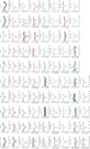 |
Fig. C.4 As Fig. C.3, but for HD 36591 (B1V). |
| In the text | |
Current usage metrics show cumulative count of Article Views (full-text article views including HTML views, PDF and ePub downloads, according to the available data) and Abstracts Views on Vision4Press platform.
Data correspond to usage on the plateform after 2015. The current usage metrics is available 48-96 hours after online publication and is updated daily on week days.
Initial download of the metrics may take a while.