| Issue |
A&A
Volume 707, March 2026
|
|
|---|---|---|
| Article Number | A157 | |
| Number of page(s) | 20 | |
| Section | Stellar structure and evolution | |
| DOI | https://doi.org/10.1051/0004-6361/202558014 | |
| Published online | 03 March 2026 | |
Massive stars exploding in a He-rich circumstellar medium
XII. SN 2024acyl: A fast, linearly declining Type Ibn supernova with early flash-ionisation features
1
Yunnan Observatories, Chinese Academy of Sciences Kunming 650216, P.R. China
2
International Centre of Supernovae, Yunnan Key Laboratory Kunming 650216, P.R. China
3
INAF – Osservatorio Astronomico di Padova Vicolo dell’Osservatorio 5 35122 Padova, Italy
4
Department of Astronomy, Kyoto University, Kitashirakawa-Oiwake-cho, Sakyo-ku Kyoto 606-8502, Japan
5
South-Western Institute for Astronomy Research, Yunnan University Kunming 650500, P.R. China
6
Yunnan Key Laboratory of Survey Science, Yunnan University, Kunming Yunnan 650500, P.R. China
7
School of Astronomy and Space Science, University of Chinese Academy of Sciences Beijing 100049, P.R. China
8
National Astronomical Observatories, Chinese Academy of Sciences Beijing 100101, P.R. China
9
School of Electronic Science and Engineering, Chongqing University of Posts and Telecommunications Chongqing 400065, P.R. China
10
INAF – Osservatorio Astronomico di Brera Via E. Bianchi 46 23807 Merate (LC), Italy
11
INAF – Osservatorio Astronomico d’Abruzzo Via M. Maggini snc 64100 Teramo, Italy
12
Department of Astronomy, University of California Berkeley CA 94720-3411, USA
13
School of Physics, O’Brien Centre for Science North, University College Dublin Belfield Dublin 4, Ireland
14
European Southern Observatory Alonso de Córdova 3107 Casilla 19 Santiago, Chile
15
Millennium Institute of Astrophysics (MAS) Nuncio Monseñor Sòtero Sanz 100 Providencia Santiago 8320000, Chile
16
Department of Physics and Astronomy, Aarhus University Ny Munkegade 120 DK-8000 Aarhus C, Denmark
17
Graduate Institute of Astronomy, National Central University 300 Jhongda Road 32001 Jhongli, Taiwan
18
Institute of Space Sciences (ICE, CSIC), Campus UAB, Carrer de Can Magrans s/n E-08193 Barcelona, Spain
19
Xinjiang Astronomical Observatory, Chinese Academy of Sciences, Urumqi Xinjiang 830011, P.R. China
20
Department of Particle Physics and Astrophysics, Weizmann Institute of Science 76100 Rehovot, Israel
21
Institut d’Estudis Espacials de Catalunya (IEEC) 08860 Castelldefels Barcelona, Spain
22
Astronomical Observatory, University of Warsaw Al. Ujazdowskie 4 00-478 Warszawa, Poland
23
Cardiff Hub for Astrophysics Research and Technology, School of Physics & Astronomy, Cardiff University, Queens Buildings The Parade Cardiff CF24 3AA, UK
24
Finnish Centre for Astronomy with ESO (FINCA), Quantum, University of Turku Vesilinnantie 5 FI-20014 Turku, Finland
25
Tuorla Observatory, Department of Physics and Astronomy, University of Turku FI-20014 Turku, Finland
26
Department of Physics & Astronomy, University of Turku Vesilinnantie 5 Turku FI-20014, Finland
27
The Oskar Klein Centre, Department of Astronomy, Stockholm University AlbaNova SE-10691 Stockholm, Sweden
28
Nordic Optical Telescope, Aarhus Universitet, Rambla José Ana Fernández Pérez 7, local 5, E-38711 San Antonio Breña Baja Santa Cruz de Tenerife, Spain
29
Department of Physics and Astronomy, University of Turku FI-20014 Turku, Finland
30
School of Sciences, European University Cyprus Diogenes Street Engomi 1516 Nicosia, Cyprus
31
School of Physics and Astronomy, University of Leicester University Road Leicester LE1 7RH, UK
32
School of Physics, Trinity College Dublin, The University of Dublin Dublin 2, Ireland
33
Instituto de Ciencias Exactas y Naturales (ICEN), Universidad Arturo Prat Iquique, Chile
34
Department of Physics and Astronomy, University of Turku FI-20014 Turku, Finland
35
Aalto University Metsähovi Radio Observatory Metsähovintie 114 02540 Kylmälä, Finland
36
Aalto University Department of Electronics and Nanoengineering PO BOX 15500 FI-00076 AALTO, Finland
37
Center for Astrophysics and Cosmology, University of Nova Gorica Vipavska 11c 5270 Ajdovščina, Slovenia
38
Instituto de Alta Investigación, Universidad de Tarapacá Casilla 7D Arica, Chile
39
INAF – Osservatorio Astronomico di Capodimonte Salita Moiariello 16 80131 Napoli, Italy
40
Department of Physics, University of Oxford, Denys Wilkinson Building Keble Road Oxford OX1 3RH, UK
41
Astrophysics Research Centre, School of Mathematics and Physics, Queen’s University Belfast Belfast BT7 1NN, UK
42
Department of Physics, Tsinghua University Beijing 100084, P.R. China
43
National Astronomical Observatory of Japan, National Institutes of Natural Sciences 2-21-1 Osawa Mitaka Tokyo 181-8588, Japan
44
Dipartimento di Fisica “Ettore Pancini”, Università di Napoli Federico II Via Cinthia 9 80126 Naples, Italy
45
Purple Mountain Observatory, Chinese Academy of Sciences Nanjing 210023, P.R. China
★ Corresponding authors: This email address is being protected from spambots. You need JavaScript enabled to view it.
, This email address is being protected from spambots. You need JavaScript enabled to view it.
, This email address is being protected from spambots. You need JavaScript enabled to view it.
Received:
7
November
2025
Accepted:
22
January
2026
Abstract
We present a photometric and spectroscopic analyses of the Type Ibn supernova (SN) 2024acyl. It rises to an absolute magnitude peak of Mo = −17.58 ± 0.15 mag in 10.6 days, and displays a rapid linear post-peak light-curve decline in all bands (e.g. γ0 − 60(V) = 0.097 ± 0.002 mag day−1), similar to most SNe Ibn. The optical pseudobolometric light curve peaks at (3.5 ± 0.8)×1042 erg s−1, with a total radiated energy of (5.0 ± 0.4)×1048 erg. The spectra are dominated by a blue continuum at early stages, with narrow P-Cygni He I lines and flash-ionisation emission lines of C III, N III, and He II. The P-Cygni He I features gradually evolve and become emission-dominated in late-time spectra. The Hα line is detected throughout the entire spectral evolution, which indicates that the circumstellar material (CSM) is helium-rich with some residual amount of hydrogen. Our multi-band light-curve modelling yields estimates of the ejecta mass of Mej = 0.49+0.11−0.09 M⊙ with a kinetic energy of Ek = 0.06+0.01−0.01 × 1051 erg, and a 56Ni mass of MNi = 0.018 M⊙. The inferred CSM properties are characterised by a mass of MCSM = 0.51+0.05−0.04 M⊙, an inner radius of R0=17.8+3.6−3.0 AU, and a density of ρCSM = (8.3+2.7−1.2) × 10−12 g cn−3. The multi-epoch spectra are well reproduced by the CMFGEN/ he4p0 model, corresponding to a He-ZAMS mass of 4 M⊙ (H-ZAMS mass 18.11 M⊙, pre-SN mass 3.16 M⊙). These findings are consistent with a scenario of an SN powered by ejecta-CSM interaction originating from a low-mass helium star that evolved within an interacting binary system where the CSM with some residual hydrogen may originate from the mass-transfer process. We also discuss an extreme scenario involving the possible merger of a helium white dwarf. In addition, a channel of core-collapse explosion of a late-type Wolf-Rayet (WR) star with hydrogen, or a transitional star between an Of and a WR type (e.g. an Ofpe/WN9 star) with fallback accretion cannot be entirely ruled out.
Key words: circumstellar matter / supernovae: general / supernovae: individual: SN 2024acyl
© The Authors 2026
 Open Access article, published by EDP Sciences, under the terms of the Creative Commons Attribution License (https://creativecommons.org/licenses/by/4.0), which permits unrestricted use, distribution, and reproduction in any medium, provided the original work is properly cited.
This article is published in open access under the Subscribe to Open model. This email address is being protected from spambots. You need JavaScript enabled to view it. to support open access publication.
1. Introduction
Type Ibn supernovae (SNe Ibn) represent a subtype of stellar explosions distinguished by relatively narrow (∼1000 km s−1) helium emission lines and weak (or no) evidence of hydrogen lines in their spectra, suggesting the presence of He-rich circumstellar material (CSM; Smith 2017; Gal-Yam 2017). SN 1999cq was the first SN Ibn identified with typical Type Ib spectral features superimposed with the narrow He I lines (Matheson et al. 2000); however, the formal designation of this new SN type was introduced by Pastorello et al. (2008a), after the study of the prototypical Type Ibn SN 2006jc (e.g. Foley et al. 2007; Pastorello et al. 2007; Anupama et al. 2009). This class is defined by analogy with SNe IIn, which show relatively narrow H lines with full width half maximum intensity (FWHM) velocities ranging from a few hundred to ∼1000 km s−1, arising from the interaction of SN ejecta with the surrounding dense H-rich CSM (Schlegel 1990; Filippenko 1997; Fraser 2020).
A few SNe Ibn have displayed transitional spectra between classical Type Ibn and IIn SNe, with H and He I lines having comparable strengths. This small sample of Type Ibn and IIn events includes SNe 2005la (Pastorello et al. 2008b), 2010al (Pastorello et al. 2015a), 2011hw (Smith et al. 2012; Pastorello et al. 2015a), 2020bqj (Kool et al. 2021), and 2021foa (Reguitti et al. 2022; Farias et al. 2024; Gangopadhyay et al. 2025). Their moderately rich CSM suggests a continuity in properties between SNe Ibn and SNe IIn (Smith et al. 2012; Pastorello et al. 2015a; Reguitti et al. 2022).
Other markers indicating the presence of CSM are the very short duration (≤10 days), narrow high-ionisation emission lines detected in very young SNe of various types (e.g. Gal-Yam et al. 2014; Shivvers et al. 2015; Khazov et al. 2016; Yaron et al. 2017; Zhang et al. 2023, 2024; Bostroem et al. 2023). These features are directly related to the effects of the shock breakout and arise from the recombination of the flash-ionised CSM (e.g. Gal-Yam et al. 2014; Yaron et al. 2017) and the interaction with a dilute wind inside the dense shell (Fransson et al. 1996). To date, only a handful of Type Ibn events have occasionally been observed with flash signatures, including SNe 2010al (Pastorello et al. 2015a), 2019cj (Wang et al. 2024b), 2019uo (Gangopadhyay et al. 2020), 2019wep (Gangopadhyay et al. 2022), and 2023emq (Pursiainen et al. 2023).
Although SNe Ibn exhibit some diversity in their spectra, they typically display an overall photometric homogeneity (see e.g. Pastorello et al. 2016; Hosseinzadeh et al. 2017; Wang et al. 2025; Dong et al. 2025). The light curves of SNe Ibn typically exhibit fast rise times (∼7 days), rapid post-peak declines (0.05–0.15 mag day−1), and luminous peak absolute magnitudes (M ≈ −19 mag). However, several outliers exist, such as the slow-rising OGLE-2014-SN-131 (Karamehmetoglu et al. 2017), the highly luminous ASASSN-14ms (MV ≈ −20.5 mag; Vallely et al. 2018; Wang et al. 2021b), the double-peaked iPTF13beo (Gorbikov et al. 2014), and the long-lasting OGLE-2012-SN-006 (Pastorello et al. 2015d). The diversity in these observational photometric and spectroscopic properties may indicate a variety of progenitor systems and explosion mechanisms for SNe Ibn.
The progenitors of SNe Ibn are usually believed to be massive (17–100 M⊙) stars, such as H-poor Wolf-Rayet (WR) stars (e.g. Foley et al. 2007; Pastorello et al. 2007; Tominaga et al. 2008; Maeda & Moriya 2022), or for individual SNe Ibn showing H lines, stars transitioning from luminous blue variable (LBV) to WR stages (e.g. Smith et al. 2012; Pastorello et al. 2015a; Reguitti et al. 2022). Although a popular scenario suggests that these are the core-collapse (CC) explosions of very massive stars embedded in helium-rich CSM, there are still many open questions concerning the homogeneity of Type Ibn progenitors. For example, SNe Ibn have usually been observed in star-forming environments (Taddia et al. 2015; Pastorello et al. 2015a), and thus the massive-star progenitor scenario is favoured. However, this association was challenged by SN Ibn PS1-12sk, which occurred in the outskirts of an elliptical galaxy CGCG 208-042 with no obvious star-formation activity (Sanders et al. 2013).
In addition to the massive-star scenario, multiple alternative progenitor models are plausible to interpret the observables of Type Ibn events. Based on observations of host-galaxy environments and inspection of explosion sites, lower-mass interacting binaries have also been proposed as progenitor systems (e.g. PS1-12sk, SN 2016jc, and SN 2015G; Sanders et al. 2013; Maund et al. 2016; Hosseinzadeh et al. 2019; Sun et al. 2020); see, in addition, Wu & Fuller (2022) and Tsuna et al. (2024). Dessart et al. (2022) performed numerical simulations to model SN Ibn spectra, suggesting that a fraction of them can be produced by the explosion of helium-star progenitors exploding in dense CSM. Moriya et al. (2025) proposed that some SNe Ibn may stem from ultrastripped SN progenitors that lose substantial mass shortly before their explosion, as a result of violent silicon burning. Metzger (2022) proposed that merger-driven destruction of WR stars rather than a CC explosion can produce SN Ibn observables. This ‘explosion’ is actually a disc outflow from the hyperaccretion onto the compact object of the He star. Since the diversity of SNe Ibn is broad, it is perhaps likely that these events originate from multiple formation channels.
In this work, we present a detailed analysis of the photometric and spectroscopic observations of SN 2024acyl, an SN Ibn with a linearly declining light curve and early flash-ionisation features. The paper is organised as follows. Section 2 outlines the discovery, distance, and extinction estimates. The photometric and spectroscopic analysis are presented in Sections 3 and 4, respectively. Our main results are discussed in Section 5, and the conclusions are drawn in Section 6.
2. Discovery, distance, and extinction
Type Ibn SN 2024acyl (also known as ATLAS24qxm, GOTO24iwf, and PS24mlb) was first detected by the Asteroid Terrestrial-impact Last Alert System (ATLAS; Tonry et al. 2018; Smith et al. 2020; Shingles et al. 2021), on 2024 December 1 UTC (MJD = 60645.28887; UTC dates are used throughout the paper) at the cyan filter magnitude of c = 18.307 mag (AB mag; Tonry et al. 2024). Early spectra of SN 2024acyl exhibit prominent He IIλ4686 and narrow He Iλ5876 emission lines; hence, it was classified as a young Type Ibn SN with flash features by Santos et al. (2024) via the extended Public European Southern Observatory (ESO) Spectroscopic Survey of Transient Objects (ePESSTO+; Smartt et al. 2015).
SN 2024acyl (RA =  , Dec =
  ; J2000) has a projected offset of 34 kpc from the core of its probable host galaxy CGCG 505-052, and is 22
 98 south and 54
 59 east of the galaxy centre (see Fig. 1). We adopted the host-galaxy redshift from NASA/IPAC Extragalactic Database (NED1) database, z = 0.026532 ± 0.000017 (Springob et al. 2005), which corresponds to a luminosity distance of dL = 111.2 ± 7.7 Mpc and a distance modulus of μL = 35.23 ± 0.15 mag. These values are calculated under the assumption of a standard ΛCDM cosmology with H0 = 73 km s−1 Mpc−1, ΩM = 0.27, and ΩΛ = 0.73 (Spergel et al. 2007). The Milky Way extinction towards SN 2024acyl is E(B − V)MW= 0.126 mag (Schlafly & Finkbeiner 2011), while the extinction within the host galaxy cannot be firmly constrained owing to the limited spectral resolution and the modest signal-to-noise ratio (S/N) of the SN spectra. Thus, we assume that the total line-of-sight extinction of SN 2024acyl is equal to the Galactic value, E(B − V)Total = 0.126 mag, an assumption also supported by the remote location of the SN from the host-galaxy core (see Fig. 1). For a detailed analysis of the host environment of SN 2024acyl, we refer to Dong et al. (2025).
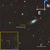 |
Fig. 1. SN 2024acyl in a NOT+ALFOSC coloured image taken with Johnson B, V, and Sloan r band filters on 2025 January 6. The SN is marked at the crosshair, near the centre of the image. |
3. Photometry
3.1. Photometric observations
Soon after the discovery announcement of SN 2024acyl, we launched a comprehensive multi-band follow-up campaign in the framework of the ePESSTO programme, the Nordic Optical Telescope (NOT) Unbiased Transient Survey 2 (NUTS22), and other programs. We collected ultraviolet (UV) and optical photometric data with the facilities listed in Table A.1 (Appendix A).
Swift/UVOT UV and optical data were retrieved from the NASA Swift Data Archive3 and measured with the standard UVOT data-reduction pipeline HEASoft4 (version 6.19, Nasa High Energy Astrophysics Science Archive Research Center (Heasarc) 2014). The optical photometric data observed from ground-based telescopes were reduced with the dedicated ecsnoopy5 pipeline, following standard procedures as described by Cai et al. (2018). In addition, the 1.6 m Multi-Channel Photometric Survey Telescope (Mephisto) magnitudes were measured following the methodology presented by Chen et al. (2024) and Zou et al. (2026). We also retrieved archival data from public surveys such as ATLAS and Pan-STARRS (e.g. Chambers et al. 2016; Flewelling et al. 2020; Magnier et al. 2020a). ATLAS orange (o) and cyan (c) magnitudes were processed through the ATLAS Forced Photometry service6 (Shingles et al. 2021), while Pan-STARRS1 (PS1) magnitudes were generated with the PS1 Image Processing Pipeline (IPP; Waters et al. 2020; Magnier et al. 2020a,b,c). The final UV and optical magnitudes of SN 2024acyl are published at the Strasbourg astronomical Data Centre.
3.2. Photometric evolution
The multi-band light curves of SN 2024acyl are shown in Fig. 2. Although its discovery was announced by ATLAS on 2024 December 1 (MJD = 60645.29), an earlier detection on 2024 November 28 (MJD = 60642.39) is recovered in archival images. While the post-maximum decline is well observed, the pre-maximum evolution is only sparsely covered by the ATLAS o- and c-band data. Therefore, the explosion time of SN 2024acyl is estimated from the midpoint between the last non-detection (MJD = 60641.39 in the c band) and the first detection (MJD = 60642.39 in the c band), yielding MJD = 60641.9 ± 0.5 days.
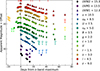 |
Fig. 2. Ultraviolet and optical light curves of SN 2024acyl. The dashed vertical line indicates the time of the o-band maximum light as the reference epoch. The vertical red lines at the top mark spectral observational epochs. The upper limits are plotted with empty symbols with arrows. The light curves for different filters are shifted with arbitrary constants, reported in the legend. The Mephisto u- and v-band data points in its unique filter system (for details see Chen et al. 2024; Yang et al. 2024) are indicated by uM and vM in the legend. Magnitude errors are usually smaller than the symbol size. |
To determine the properties of SN 2024acyl at peak brightness, we performed a polynomial fit on the o-band light-curve data around the maximum (±12 days), which provides a peak magnitude of 17.66 ± 0.02 mag and a peak time of MJD = 60652.49 ± 0.26. We adopted this epoch as a reference time. The fitting uncertainties were estimated via Monte Carlo simulations. The light curves of SN 2024acyl are asymmetric, with a relatively long rise (∼10.6 days) to maximum light, but a fast and linear post-peak decline. We used a linear fit to determine the post-peak decline rates in all bands. The fitted values, which provide a comparison of the fading behaviour across various filters, are reported in Table 1. Given the relatively noticeable changes in the slope of the light curves of SN 2024acyl at approximately +25 days and +45 days, we estimated the decline rates across three distinct time intervals. SN 2024acyl has a rapid decline compared with other Type Ibn SNe during the whole post-peak evolution in all bands, with the blue-band light curves declining faster than those in the red bands (e.g. two extreme bands of UVW2 and z in the first 25 days: γ0 − 25(UVW2) = 19.8 ± 1.03 mag (100 d)−1; γ0 − 25(z) = 7.98 ± 0.36 mag (100 d)−1). From 25 d to 45 d, the light curves decline slower for those bands that are visible, with a sort of pseudoplateau (e.g. γ25 − 45(B) = 5.89 ± 0.45 mag (100 d)−1; γ25 − 45(z) = 5.29 ± 0.33 mag (100 d)−1.) Later, the light curve steepens again with a decline rate of γ≥45(z) = 8.30 ± 2.23 mag (100 d)−1 until the last detection at about +70 days.
Decline rates of the multi-band light curves of SN 2024acyl, along with their uncertainties, in units of mag (100 d)−1.
The colour evolution of SN 2024acyl is shown in Fig. 3, compared with those of a selected sample of Type Ibn SNe, including the prototypical Type Ibn SN 2006jc and a few objects7 that share similar light-curve properties with SN 2024acyl. In the top panel of Fig. 3, the B − V colour becomes red very rapidly, moving from a blue colour of +0.0 mag at −5 days to a red one of +0.8 mag at +30 days. After maximum brightness, the B − V colour turns bluer to +0.4 mag in the following days up to +55 days. However, the comparison objects reveal that there is diversity in the colour evolution of SNe Ibn. The B − V colour of SNe 2010al and 2019cj become redder rapidly at their early stages resembling that of SN 2024acyl, but the later evolution turns to moderately redder colours. SN 2019kbj shows a similar trend but its colour is bluer. SN 2006jc evolves to a blue colour from −0.1 mag to −0.4 mag in its first +15 days and gradually becomes redder at around −0.2 mag (with minor fluctuations) until day +60. Subsequently, it rapidly became redder, which is likely to associated with dust formation (Mattila et al. 2008; Smith et al. 2008; Di Carlo et al. 2008). In the bottom panel of Fig. 3, the r − i colour of SN 2024acyl slowly increases from −0.2 mag at ∼0 day to +0.1 mag at +15 days and subsequently settles to about +0.3 mag (+51 days) but with some fluctuations. We caution that there is also the possibility that fluctuations in the colour curves are likely due to data quality and are not of the SN. The evolution of the R − I/r − i colour in the comparison objects is consistent with the trend seen in SN 2024acyl within the observed time window, although the colour of SN 2006jc becomes much redder at late phases.
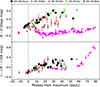 |
Fig. 3. Colour evolution of SN 2024acyl compared with the prototypical Type Ibn SN 2006jc and other fast, linearly declining SNe Ibn. Top panel: B − V colours. Bottom panel: R − I or r − i colours. The colour curves have been corrected for galactic extinction. |
Adopting the distance and reddening estimates reported in Sec. 2, SN 2024acyl reached absolute magnitudes of MB = −18.02 ± 0.15 mag, Mg = −18.13 ± 0.15 mag, MV = −18.14 ± 0.15 mag, Mo = −17.88 ± 0.15 mag, and Mi = −17.82 ± 0.15 mag. Only upper limits can be estimated for other bands owing to the incomplete data coverage around maximum: Mr < −18.04 mag and Mz < −17.59 mag. SN 2024acyl is slightly fainter than the average absolute magnitude of SNe Ibn (Mr ≈ −19 mag; Pastorello et al. 2016; Hosseinzadeh et al. 2017; Wang et al. 2025), and much fainter than the highly luminous ASASSN-14ms (MV ≈ −20.5 mag; Vallely et al. 2018; Wang et al. 2021b). On the other hand, SN 2024acyl is much brighter than SN 2023utc, which is the faintest Type Ibn SN reported in the literature (Mr = −16.4 ± 0.5 mag; Wang et al. 2025). To highlight the fast and linear post-peak photometric decline of SN 2024acyl, we compared the r-band light curve of SN 2024acyl with those of a few representative SNe Ibn and the Type Ibn templates presented by Hosseinzadeh et al. (2017) and Khakpash et al. (2024) (see Fig. 4). The light curve of SN 2024acyl declines rapidly at phases later than +5 days, consistent with most SNe Ibn (including SNe 2006jc and 2020nxt), and it follows the behaviour of the templates released by Hosseinzadeh et al. (2017). However, SN 2024acyl before +5 days is less luminous than other SNe Ibn whose peak absolute magnitudes range from −18.9 mag to −20.5 mag, with the notable exception of SN 2023utc.
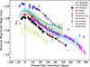 |
Fig. 4. Light curves in the V-band of SN 2024acyl, including the comparison SNe Ibn. Template V-band light curves for Type Ibn SNe are from Hosseinzadeh et al. (2017, blue) and Khakpash et al. (2024, green). Due to data-coverage limitations, SN 2023utc is represented using r-band photometry converted to the Vega system. |
To make a meaningful comparison of SN 2024acyl with other SNe Ibn, we constructed their pseudobolometric light curves based on the photometry available in the same set of filters, from the B to the I/i bands. Therefore, we first converted extinction-corrected magnitudes to flux densities, and then integrated the spectral energy distribution (SED) within their effective wavelengths. In our computation, we made the assumption that the flux contribution outside the integration limits, which represent the coverage of each bands, is zero. Occasionally, when some photometric data in a given filter were not available, we interpolated or extrapolated the missing flux from the nearest available photometry assuming a constant colour evolution.
The resulting pseudobolometric light curves of SN 2024acyl and the compared SNe Ibn are shown in Fig. 5. The pseudobolometric light curve of SN 2024acyl is broadly similar to other Type Ibn events. The peak ‘optical’ luminosity of SN 2024acyl, (3.5 ± 0.8)×1042 erg s−1, is between those of most SNe Ibn (∼3–20 × 1042 erg s−1) and the faintest SN 2023utc (∼7.1 × 1041 erg s−1). The peak ‘UV+Optical’ luminosity, (6.7 ± 0.4)×1042 erg s−1, of SN 2024acyl is still fainter than that of ASASSN-14ms (∼2.3 × 1043 erg s−1). We observed a significant difference in peak luminosity between the ‘optical’ and ‘UV+Optical’ results. This indicates that the contribution from UV bands is significant during the early phases, which is consistent with observations of other SNe Ibn (see Wang et al. 2024a,b). Such a feature suggests a high-temperature scenario in the early phases where the peak of the SED falls within the UV bands (e.g. when TBB = 20 000 K, λmax ≈ 1500 Å). Furthermore, strong interaction may generate energetic photons; as the ejecta are opaque to this radiation in the early phases, these photons are thermalised into softer UV emission. These factors combined explain the high contribution of UV bands in the early phases, consistent with the work of Maeda & Moriya (2022). In addition, we estimated the radiated energies of SN 2024acyl from the ‘optical’ and ‘UV+Optical’ pseudobolometric light curves, using a non-parametric fit of a ReFANN8 code (see details in Wang et al. 2020a,b, 2021a). The resulting radiated energies integrated with the entire photometric evolution time are (5.0 ± 0.4)×1048 erg and (8.5 ± 0.6)×1048 erg, respectively. These values of SN 2024acyl are within the range of (1–32)×1048 erg, as reported for the typical Type Ibn sample (see Table 2 of Wang et al. 2025). Note that these values should be considered lower limits owing to limited temporal and wavelength coverage.
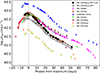 |
Fig. 5. Pseudobolometric light curves of SN 2024acyl and the comparison SNe Ibn. The comparison objects have luminosities comparable to that of the ‘optical’ luminosity of SN 2024acyl, integrating from the B to the I/i bands. |
3.3. multi-band light-curve modelling
Type Ibn SNe are characterised by strong interaction between their ejecta and a helium-rich CSM (Karamehmetoglu et al. 2017; Kool et al. 2021; Pellegrino et al. 2022). This ejecta-CSM interaction (CSI) is a dominant power source for the light curve, necessitating a more complex model than one based solely on radioactive decay (RD). Therefore, to accurately model the light curve of SN 2024acyl, we adopted a hybrid model that combines contributions from both RD and CSI, following Chatzopoulos et al. (2012).
We adopted the MOSFiT Monte-Carlo fitting code (Guillochon et al. 2018), widely used in other Type Ibn SNe (e.g. Kool et al. 2021; Farias et al. 2024), to fit the multi-band light curve of SN 2024acyl. The bands we used to constrain the explosion parameters here were the UV plus the optical uMvMBgcVroiz ones. The data in the uM and vM bands (for which the effective wavelengths are 3454 Å and 3854 Å, respectively) are taken from the Mephisto survey with its unique filter system, which has better coverage around the peak and in the post-maximum phases. Using MOSFiT, we obtained the posterior distribution of each parameter along with its uncertainty, and inspected the degeneracy between different parameters. Furthermore, by fitting the light curve of each band independently using MOSFiT, we can accurately model the colour evolution of SN 2024acyl. This approach is particularly effective for the refined uM- and vM- bands from the Mephisto survey.
The RD-CSI model implemented in the MOSFiT code is based on the formalism of Chatzopoulos et al. (2012). In this semi-analytical framework, the luminosity, L(t), is computed as the diffusion of an energy input through the ejecta:
![Mathematical equation: $$ \begin{aligned} \begin{split} L(t) = \left[\frac{1}{t_0} e^{-\frac{t}{t_0}}\int _{0}^{t}\mathrm{d}\tau \, e^{\frac{\tau }{t_0}}L_{\mathrm{inp}}(\tau )+\frac{E_{\rm init}}{t_0}e^{-\frac{t}{t_0}}\right] \\ \times \left(1-e^{-\kappa _\gamma \rho (t)R(t)} \right) \, . \end{split} \end{aligned} $$](/articles/aa/full_html/2026/03/aa58014-25/aa58014-25-eq10.gif) (1)
(1)
Here, t0 = κMej/βcvph is the characteristic diffusion timescale, where β ≈ 13.8 is an integration constant derived from the diffusion model (see e.g. Arnett 1982; Valenti et al. 2008). The input energy source, Linp(τ), is the sum of RD and CSI. The RD component is powered by the RD chain 56Ni→56Co→56Fe. The CSI component consists of contributions from both a forwards and a reverse shock, the strengths of which depend on the density profiles of the ejecta and the surrounding CSM (Chevalier 1982). The model is described by several key parameters. The diffusion process is primarily governed by the 56Ni fraction (f56Ni), the ejecta mass (Mej), the ejecta kinetic energy (Ek), the optical opacity (κ), and the gamma-ray opacity (κγ, which accounts for gamma-ray leakage). The CSI is characterised by the CSM mass (MCSM), its inner radius (R0), and parameters describing the density profiles of the CSM (s) and the ejecta (n, δ). The CSM density profile is expressed as ρCSM ∝ r−s, where s = 2 corresponds to a steady stellar wind, while s = 0 represents a dense, shell-like CSM with constant density. Additionally, the MOSFiT fitting process includes some additional parameters including the explosion time (texp), a minimum photospheric temperature (Tmin), and an uncertainty term (σ) added in quadrature to the observational errors to account for model uncertainties, which indicate the fitting quality.
The complexity of the RD-CSI model and the high dimensionality of its parameter space make the fitting process computationally challenging. To simplify the problem, we fixed several parameters or use more restrictive priors based on physically motivated assumptions. Given that the fitting results are insensitive to the density profile of the ejecta (see Villar et al. 2017; Kool et al. 2021; Farias et al. 2024), we use restrictive priors for these parameters. For the density profile of the inner ejecta, we adopt a constant-density profile (δ = 0; Wang et al. 2025). Regarding the density profile of the stellar envelope, Chatzopoulos et al. (2012) noted that for the relatively compact scenario, the index n needs to be smaller; specifically, n ≲ 10 for BSG and WR cases, which represent a radiative envelope, in contrast with the convective envelope of RSG stars (n ≈ 12). Furthermore, Farias et al. (2025) noted that for the RD+CSI hybrid model, the best-fit n is approximately 9. Conversely, Kool et al. (2021) and Wang et al. (2025) fixed n = 12 as a standard value, as it does not significantly affect the result. Thus, considering all these scenarios, we adopted n = 10 and n = 12, which represent compact and generally used cases, respectively. For the density profile of the CSM, we considered two scenarios: s = 0 and s = 2. The former represents a shell-like CSM driven by strong WR winds or eruptive mass-loss events, while the latter represents a steady stellar wind (Chatzopoulos et al. 2012). We also adopted a constant optical opacity of κ = 0.1 cm2 g−1, typical for helium-rich ejecta (Prentice et al. 2019), and a gamma-ray opacity of κγ = 0.027 cm2 g−1. This procedure reduced the number of free parameters in our fit to eight: f56Ni, Mej, Ek, MCSM, ρCSM, R0, Tmin, and the additional uncertainty term σ. Given the potential for a complex posterior distribution and the high-dimension parameter space, we employed the nested sampling algorithm implemented in the dynesty package (Speagle 2020) instead of traditional ensemble-based samplers. We initialised the sampler with 120 live points (‘walkers’) and ran the algorithm iteratively until the stopping criterion was reached to ensure the good convergence of the samplers.
The best-fit model is presented in Fig. 6, overlaid on the multi-band photometric data9. The corresponding model parameters are listed in Table B.1 (Appendix B). All parameters were constrained by the observational data, with uncertainties defined by the 68% (∼1σ) confidence intervals of their posterior distributions. The additional uncertainty added to the observation data is ∼0.15 mag in this fitting, consistent with the large-sample analysis of Wang et al. (2025).
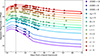 |
Fig. 6. Fits to the multi-band light curves of SN 2024acyl with n = 10, δ = 0, and s = 0 using the MOSFiT Monte Carlo code with the hybrid Ni+CSM model. For each filter, a subset of randomly sampled model light curves from the posterior distributions are displayed to illustrate the uncertainty of the model fits. |
Therefore, the results should be regarded as indicative and used with caution. The minimum photospheric temperature, Tph, min, is not listed, as the model is insensitive to this parameter compared to other key parameters (Nicholl et al. 2017). The corner plot, illustrating the posterior distributions and the degeneracies between parameters, is shown in Fig. D.1 in Appendix D.
We found that for both n = 12 and n = 10, the models with s = 0 provide tighter constraints on the parameters compared to the s = 2 models. Furthermore, the Bayesian evidence of the s = 0 models is approximately log𝒵 ≈ 304, whereas the s = 2 models yield log𝒵 ≈ 296. This indicates that the s = 0 models are statistically favoured. The value of n does not significantly affect the key parameters; both n = 12 and n = 10 yield similar low-mass solutions (with consistent MCSM and density) and share comparable Bayesian evidence (Δlog𝒵 ≲ 1), which is consistent with Kool et al. (2021) and Wang et al. (2025). Considering these findings, we indicate that the posterior distributions of the parameters are well constrained.
As presented in Fig. D.1, Mej and Ek are degenerate. Thus, we can robustly constrain the Mej ≲ 1 M⊙ and Ek ≲ 0.1 × 1051 erg. The choice of the density profile index n introduces a systematic uncertainty of ∼0.2 M⊙ for Mej and ∼0.02 × 1051 erg for Ek. By considering that most SNe Ibn exploded from relatively compact progenitors, we take the posterior of n = 10 scenario as a reasonable result. The best-fit values are  and
and  for SN 2024acyl. The value of Mej is comparable to those of other Type Ibn SNe such as PS1-12sk (∼0.3 M⊙; Sanders et al. 2013), located at the lower end of the Mej distribution of SNe Ibn. The value of Ek is reasonable because it falls in the low-energy tail of SNe Ibn, which is (0.06 − 0.91)×1051 erg. However, we caution that these are correlated, as a higher ejecta mass results in a higher kinetic energy, and vice versa.
The derived properties of the CSM are also typical of SNe Ibn. The CSM properties are not significantly affected by the choice of n, which implies that they are robust against variations in the density profile. The MCSM of SN 2024acyl is  , which is comparable to that of iPTF15ul and SN 2019uo with the assumption of shell-like CSM (s = 0) (∼0.3–0.7 M⊙; Pellegrino et al. 2022; Gangopadhyay et al. 2020). The best-fit inner radius of the CSM of SN 2024acyl is
  , which falls within the observed range of 9 − 60 AU, bracketed by examples such as SN 2020nxt (∼9 AU; Wang et al. 2025) and iPTF15ul (∼60 AU; Pellegrino et al. 2022). The posterior CSM density for SN 2024acyl is
  . The CSM properties of SN 2024acyl is consistent with that of other SNe Ibn with s = 0. The outer radius of the CSM can be derived from R0, MCSM, and ρCSM, which is around 24.3 AU, indicating a relatively thin CSM with a thickness of ∼6.5 AU, suggesting eruptive mass loss of the progenitor. Therefore, the reasonable posterior distributions of the CSM parameters (e.g. R0, MCSM, and ρCSM), and the higher Bayesian evidence log𝒵 ≈ 304 for s = 0 models, indicate that its properties are well constrained. The profile of the CSM can be a probe of the mass-loss history of the progenitor, as discussed in Sec. 5.
For interacting SNe, the contribution from RD is often secondary, with MNi typically being low (≲0.1 M⊙; Maeda & Moriya 2022; Ben-Ami et al. 2023). For SN 2024acyl, considering the posteriors of mass fraction of 56Ni and the ejecta mass, we find MNi = 0.018 M⊙. This value is comparable to that of SN 2019wep (0.015 ± 0.05 M⊙; Pellegrino et al. 2022) and lies within the range (0.001–0.15 M⊙) of the sample from Wang et al. (2025). Finally, we estimated a characteristic ejecta velocity using the relation  . This yields a velocity of ∼3500 km s−1 for SN 2024acyl, comparable to that of SN 2020bqj (∼3300 km s−1; Kool et al. 2021) and SN 2020taz (∼3480 km s−1; Wang et al. 2025). However, as a characteristic value, the velocity derived here may differ from the actual spectroscopic velocity and should therefore be used with caution.
4. Spectroscopy
4.1. Spectroscopic observations
Our spectroscopic observations of SN 2024acyl were obtained using multiple instrumental configurations: The 2.4 m LJT equipped with the Yunnan Faint Object Spectrograph and Camera (YFOSC; Wang et al. 2019) at Gaomeigu, Lijiang, China; the Kast double spectrograph (Miller & Stone 1993) mounted on the 3 m Shane telescope at the Lick Observatory; the 3.58 m New Technology Telescope (NTT) equipped with the ESO Faint Object Spectrograph and Camera 2 (EFOSC2; Buzzoni et al. 1984), located at La Silla, Chile; the 3.58 m Telescopio Nazionale Galileo (TNG) with the Device Optimized for the LOw RESolution (DOLORES; Molinari et al. 1997) spectrograph, hosted on La Palma, Spain; and the 8 m Gemini–North telescope equipped with Gemini Multi-Object Spectrograph (GMOS-N; Hook et al. 2004; Gimeno et al. 2016) on Mauna Kea in Hawai’i, USA. Additionally, we collected a single-epoch (2024-12-04) spectrum from the Transient Name Server (TNS10), which was obtained by Soubrouillard & Leadbeater (2024). Basic information for the spectra is reported in Table C.1 (Appendix C).
Reduction of the GMOS-N data was done by (DRAGONS Labrie et al. 2023) packages following standard procedures. The Shane/Kast spectrum was taken at or near the parallactic angle to minimise slit losses caused by atmospheric dispersion (Filippenko 1982). Its data reduction followed standard techniques for CCD frame processing and spectrum extraction (Silverman et al. 2012) using IRAF routines and custom PYTHON and IDL codes11. The NTT/EFOSC2 spectra were reduced using a dedicated pipeline PESSTO12 (Smartt et al. 2015), while spectra obtained from other instruments were processed using standard procedures in the IRAF environment. Specifically, the raw data were first pre-reduced with preliminary steps, such as bias, overscan, trimming, and flat-fielding corrections. Then, we extracted one-dimensional spectra from the two-dimensional frames. Wavelength and flux calibrations were performed using spectra of comparison lamps and spectrophotometric standard stars, respectively, which were observed during the same night and with the same instrumental configurations as the SN spectra. The wavelength-calibrated spectra were cross-checked with the night-sky emission lines, while the flux-calibrated spectra were improved by calibrating to the coeval broadband photometry. We also examined the consistency between the colours derived from synthetic photometry and the observed colour evolution. However, we noted a minor discrepancy in the data, as the difference in the g − r and r − i bands is approximately ∼0.1 mag. Since we could not determine the precise reddening parameters, we treated this discrepancy as a systematic uncertainty of the extinction in our fitting procedure. Finally, the strongest telluric absorption bands (e.g. O2 and H2O) in the SN spectra were removed using the spectra of standard stars.
4.2. Spectroscopic evolution
We collected 12 optical spectra of SN 2024acyl, spanning about 50 days and covering all crucial phases of its evolution. The spectral evolution of SN 2024acyl, as shown in Fig. 7, exhibits features typical of SNe Ibn.
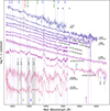 |
Fig. 7. Time sequence of SN 2024acyl spectra. Some prominent features, such as He I, He II, and N III, are marked with vertical lines, while the strongest telluric absorption bands are indicated with the ⊕ symbols. The phases reported to the right of each spectrum are from the epoch of o-band maximum light (MJD = 60652.49 ± 0.26; 2024-12-08). Spectra with a low S/N were binned with 20 Å each bin; the original (unbinned) spectra are displayed in lighter colours behind. Reddening and redshift corrections have been applied to the spectra. |
The first spectrum of SN 2024acyl was obtained on 2024 December 4 (phase ∼−3.7 days from maximum light; Soubrouillard & Leadbeater 2024). This low-S/N spectrum shows a blue, almost featureless continuum and did not provide a secure classification. A prominent bump detected at ∼4600–4700 Å is probably due to a blend of C IIIλ4648, N IIIλ4640, and He IIλ4686 emission lines. We estimated the temperature by fitting the continuum with a blackbody function. Since we noticed that the systematic error is likely to be underestimated, we introduce the jitter term as the additional error in the fitting process. The best-fit results yield a photospheric temperature of  with the additional jitter
  13. Subsequently, the second spectrum of SN 2024acyl (∼−2.4 days) supports the classification of this event as a Type Ibn SN (see Sec. 2). This spectrum is still dominated by a blue continuum (TBB = 15 000 ± 600 K), but now the He Iλ5876 line is clearly detected with a narrow P-Cygni profile. The position of the minimum of this blueshifted absorption component indicates that the velocity of the He-rich material is 1050 ± 320 km s−1. The feature detected in the first spectrum at ∼4600–4700 Å is now more prominent, and it shows a double-peaked profile. The red component is likely due to He IIλ4686, while the blue component possibly arises from a blend of N IIIλ4640 and C IIIλ4648. They are identified as flash-ionisation features, resembling those seen in other Type Ibn events, such as SNe 2010al (Pastorello et al. 2015a), 2019cj (Wang et al. 2024b), 2019uo (Gangopadhyay et al. 2020), 2019wep (Gangopadhyay et al. 2022), and 2023emq (Pursiainen et al. 2023) (see further discussion in Sec. 4.4). We note that the apparent emission bump at around 6560 Å is likely due to a blend of Hα and He IIλ6560 in these early spectra.
From −0.8 to +0.5 days after maximum light, the spectra are still dominated by blue continua with TBB decreasing from 17 500 ± 700 K to 13 100 ± 300 K. The narrow P-Cygni profiles of He Iλ5876 become progressively more prominent with measured expansion velocities of 1050−1270 km s−1. These P-Cygni features are likely produced in the He-rich CSM moving at a velocity slightly above 1000 km s−1. The feature at 4600–4700 Å gradually becomes weaker during this time window, disappearing at later phases. The following three spectra, from +0.7 days (TBB = 12 820 ± 620 K) to +1.8 days (TBB = 11 200 ± 600 K), do not show significant evolution. The measured He Iλ5876 Å P-Cygni line velocities are approximately 1280 km s−1 and 990 km s−1, respectively. The only Balmer line detected in SN 2024acyl is weak Hα, which shows minor evolution in strength during these phases.
The following spectra, from +15.6 to +42.8 days, exhibit major changes. The continua are now much redder, with a temperature decreasing from TBB = 8, 300 ± 300 K to TBB = 7, 100 ± 300 K with a similar log(σ/1042 erg s−1)≈ − 3.9. The emission components of He Iλ5876 dominate over the P-Cygni absorption starting from +15.6 days. The FWHM velocity of these broader He Iλ5876 emission lines, as obtained from a single Gaussian fit, is about 5800–6200 km s−1. The broader profile observed for all lines indicates that the SN photosphere recedes with time from the CSM to the ejecta. As shown in the bottom of Fig. 7, relatively broad features are identified in the blue region, including He Iλ3889, λ4471, λ4921, and λ5016, several Fe II multiplets (e.g. Fe II multiplet 42 lines at λλλ 4924, 5018, 5169) blended with He I emission lines, and also Mg Iλλ4571, 5528 mostly in emission. In addition, He Iλ5876, λ6678, λ7065, λ7281 evolve significantly, becoming the most prominent emission features in the red spectral region (≥5600 Å). Hα becomes more evident at late phases, blended with He Iλ6678, indicating the presence of hydrogen in the outer CSM. The near-infrarad (NIR) Ca II triplet is weak in the +18.6 day NTT/EFOSC2 spectrum, while the emission at about 7300 Å is likely a blend of [Ca II] λλ7291, 7323 and He Iλ7281. We also tentatively identify O Iλλλ7772, 7774, 7775 lines in this spectrum, following Pastorello et al. (2015c). A relatively strong bump feature detected at 9000–9400 Å is tentatively identified as a blend including Mg II (λ9218–9244). The late-time spectra of SN 2024acyl show an evident pseudocontinuum bluewards of ∼5600 Å. As suggested by Turatto et al. (1993), Smith et al. (2012), and Stritzinger et al. (2012), it is likely due to a forest of narrow and intermediate-width Fe lines, as marked in the shaded region of Fig. 7. The broad W-shape feature at 4600–5200 Å may also be attributed to Fe features blended with He I lines. All the above features are frequently observed in late-time spectra of SNe Ibn.
4.3. He I line evolution
In Fig. 8, we illustrate the temporal evolution of the He Iλ5876 line profile in SN 2024acyl (left panel). The line strength increases with time, and two distinct kinematic components can be identified. The narrow He I feature, with velocities of about 1000–1300 km s−1 as inferred from either the FWHM of the emission or the position of its weak P-Cygni absorption, arises from the slowly moving, unshocked He-rich CSM. A broader component, with a velocity of 5800–6400 km s−1, is detected in the later spectra. The coexistence of two components is consistent with an origin in two distinct regions, with the narrow P-Cygni features forming in the unperturbed CSM and the broader lines arising from the expanding ejecta. Similar evolution has been observed in the spectra of other SNe Ibn, such as ASASSN-15ed (Pastorello et al. 2015b) and SN 2010al (Pastorello et al. 2015a), where narrow lines dominate at early phases before broader ejecta signatures emerge. At early times, the photosphere lies within the dense CSM shell, above which the narrow lines form. These features are likely photoionised either by early ejecta–CSM interaction or by the initial shock breakout. As the shell recombines and becomes transparent, the underlying SN ejecta gradually dominate the spectra.
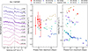 |
Fig. 8. Temporal evolution of the He Iλ5876 line. Left panel: line-profile evolution in the velocity space. The dashed vertical line marking marks the rest wavelength. Middle panel: evolution of the velocities measured from the P-Cygni absorption minimum of the narrow He I component, formed in the unshocked CSM. Right panel: evolution of the broader He I emission components, reflecting the dynamics of the shocked gas. For clarity, the uncertainties are not shown in the plots, but they can reach values of up to 30%. The comparison data for SNe Ibn are from Pastorello et al. (2016) and Wang et al. (2025). |
The middle panel of Fig. 8 shows the velocity evolution of the narrow He I component. In most SNe Ibn, these lines exhibit little or no change over time, consistent with emission from a quasistationary CSM shell. Typical velocities fall in the range 600–1500 km s−1, comparable to Wolf–Rayet wind speeds. For SN 2024acyl, the narrow-line velocity of ∼1100 km s−1 is similar to those measured in SNe 2020nxt, 2015U, and 2010al, while lower values (< 800 km s−1) are found in SNe 2005la, 2011hw, and 2006jc. This spread in velocity likely reflects differences in progenitor wind properties such as terminal velocity and mass-loss rate.
The right-hand panel of Fig. 8 illustrates the velocity evolution of the broader He I components. Unlike the narrow features, these display more pronounced temporal changes, pointing to a diversity in the ejecta kinematics and in the density structure of the shocked CSM among the SNe Ibn of the comparison sample. For example, in SN 2006jc the intermediate-width He I components narrowed from about 3100 km s−1 to 1700 km s−1 over four months, while in SN 2005la the velocities increased from ∼2000 km s−1 shortly after discovery to ∼4200 km s−1 within three weeks. However, the limited number of available spectra for SN 2024acyl prevents us from tracing a clear evolutionary trend.
4.4. Comparison with Type Ibn SN spectra
Figure 9 compares the early-time spectrum of SN 2024acyl with those of several Type Ibn events (SNe 2010al, 2019cj, 2019uo, 2019wep, and 2023emq) as well as the Type IIn SN 1998S. All spectra were obtained within a few days prior to the epoch of the maximum light. The inset highlights the region between 4400 and 5000 Å, where flash-ionisation features are most prominent. SN 2024acyl shows remarkable resemblance to other events, particularly in the simultaneous presence of flash-ionisation signatures of He II and prominent N/C lines. The detection of high-ionisation transitions, such as He IIλ4686 and N III/C IIIλλ4640, 4650, indicates the action of an external photoionisation source on the dense CSM, most likely arising from a shock breakout or the onset of ejecta–CSM interaction. Such transient flash-ionisation signatures are observed only in a subset of SNe Ibn (e.g. Pastorello et al. 2016; Gangopadhyay et al. 2020, 2022; Pursiainen et al. 2023; Wang et al. 2024b), but are well documented in the early spectra of many CC Type II SNe (Fassia et al. 2001; Gal-Yam et al. 2014; Bostroem et al. 2023; Bruch et al. 2023; Zhang et al. 2023, 2024; Jacobson-Galán et al. 2024). Furthermore, the early detection of nitrogen lines in SN 2024acyl points to the presence of CNO-processed material in the progenitor wind, thereby providing constraints on its pre-SN evolutionary state.
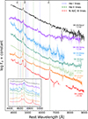 |
Fig. 9. Comparisons of the spectra of SN 2024acyl with the Type IIn SN 1998S and other Type Ibn events (SN 2010al, SN 2019cj, SN 2019uo, SN 2019wep and SN 2023emq) at their very early phases. The inset shows a close-up view of the region between 4400 Å and 5000 Å with prominent flash-ionisation features. The phases marked on the right side of each SN spectrum are with respect to the epoch of their maximum light. Spectra with a low S/N were binned with 20 Å in each bin. The original (unbinned) spectra are displayed in lighter colours behind. |
Figure 10 illustrates the spectral evolution of SN 2024acyl compared with a diverse sample of Type Ibn and IIb/Ibn events at both intermediate (+10 to +20 d; left panel) and later epochs (+50 to +100 d; right panel). The phases are related to the estimated explosion epoch, in order to make the comparisons more resonable. Around maximum light, SN 2024acyl exhibits pronounced P-Cygni profiles in He Iλλ4471, 5876, 7065, closely resembling SN 2010al at comparable phases (Pastorello et al. 2015a). Weak but clearly detectable Balmer emission lines are also present, placing SN 2024acyl within the H-bearing subset of Type Ibn events. At later phases, SN 2024acyl still maintains prominent He I emission lines with increasingly broader widths, consistent with other Type Ibn SNe. The persistent helium features, combined with the enhanced Balmer components, indicate that the CSM is primarily helium-rich, with hydrogen confined to the outermost layers. Taken together, these spectral comparisons confirm that the ejecta of SN 2024acyl interact with a dense, helium-dominated CSM that contains a residual amount of hydrogen. The spectroscopic diversity of SNe Ibn likely depends on the variety of their progenitor mass-loss histories, wind compositions, or how the stellar components in a binary system interact in the final stages before the core collapse.
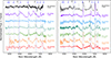 |
Fig. 10. Comparisons of the spectra of SN 2024acyl at different phases with those of the transitional Type IIb/Ibn event SN 2018gjx and several Type Ibn events with H signatures, such as SNe 2006jc, 2010al, 2011hw, 2020bqj, and PS1-12sk. Left panel: Spectra obtained at around the time of maximum light (∼10 − 20 days). Right panel: late-time spectra (∼50 − 120 days). The key spectral lines (H and He) are marked with coloured dashed lines. The phases marked on the right side of each spectrum are with respect to the epoch of their maximum light. Spectra with low S/N have been binned with 20 Å; the original (unbinned) spectra are displayed in lighter colours behind. All the phases marked in the figure are related to the (approximate) explosion epoch. |
4.5. Spectral modelling
To investigate the ejecta properties and the progenitor system of SN 2024acyl, we compared a subset of the observed spectra with a series of non-local thermodynamic equilibrium radiative-transfer models computed with CMFGEN (Hillier & Dessart 2012). These include both the models of Dessart et al. (2022) and additional tailored simulations with modified input parameters (Dessart, priv. comm.). The adopted configurations involve the interaction of moderately energetic (∼1050 erg), low-mass (≲1 M⊙) ejecta with a slowly expanding, helium-rich circumstellar envelope of a roughly comparable mass, which is compatible with our MOSFiT results. Under this condition, the analysis of the low-energy output can be simplified by concentrating on the cool dense shell (CDS), which develops as a compact, thin layer during the interaction and becomes the dominant source of radiation at later phases.
In this steady-state approximation, the hydrodynamical evolution is not explicitly modelled, and the CDS is represented as a chemically mixed layer described by a Gaussian density distribution centred at 2000 km s−1 and scaled to recover the total ejecta mass. Energy originating from both RD and residual interaction is deposited non-thermally within the CDS, enabling a consistent treatment of its ionisation and excitation conditions. Although these simulations are not designed to reproduce individual SNe in detail, they provide a valuable tool to investigate the spectral diversity and the underlying parameter degeneracies. Dessart et al. (2022) further demonstrated that similar spectral morphologies can arise from different combinations of CDS mass, radial extent, and input power.
The persistent presence of He I lines throughout the spectral evolution indicates a progenitor dominated by a helium-rich composition. Therefore, following the methodology of Wang et al. (2024a, 2025), we adopted scenarios with a helium-star progenitor. According to the helium-star evolutionary tracks of Woosley (2019), progenitors with zero-age ‘He’ main-sequence masses of 3–4 M⊙ (e.g. models he3 and he4) are consistent with the observed properties of SNe Ibn. In this work, we made use of model he4, characterised by MpreSN = 3.16 M⊙ and total ejecta mass 1.62 M⊙, comprising 0.92 M⊙ of helium, 0.31 M⊙ of oxygen, 0.03 M⊙ of magnesium, and 0.0014 M⊙ of calcium, and assuming a solar metallicity, which indicate a low-mass progenitor scenario. Figure 11 presents synthetic spectra from model he4p0 compared with observations of SN 2024acyl at multiple epochs after maximum light. We present the model comparisons of the spectra in +15.6 days, +29.6 days, and +42.8 days since the o-band maximum. To highlight the role of luminosity evolution, only the input power changes with time. Thus, we adopt the he4p0 models with 3 × 1042 erg s−1, 5 × 1041 erg s−1, and 1 × 1041 erg s−1 luminosity correspondingly, while the CDS radius (3 × 1015 cm) and velocity (2000 km s−1) were kept constant. The adopted power values are broadly consistent with the observed bolometric light curve (see Fig. 5).
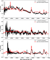 |
Fig. 11. Comparison of synthetic spectra from the he4p0 model with the observed spectra of SN 2024acyl obtained after the o-band maximum light. No smoothing has been applied to either the observed or the synthetic spectra. The synthetic spectra are based on simulations by Dessart et al. (2022) and Wang et al. (2024a), as well as on newly computed models incorporating updated parameters. The model spectra have been scaled to match the resolution of the observed spectra. |
At +15.6 d, the assumption of a narrow and homogeneous dense shell is unlikely to be valid. Relative to SN 2024acyl, the models systematically overpredict the strengths of the He I lines (see the top panel of Fig. 11). At +29.6 d and +42.8 d, the He I profiles predicted by the models exhibit a blue-red asymmetry and a central absorption dip (see Fig. 11, middle and bottom panels). However, the observations of SN 2024acyl reveal a He I line with a single, rounded peak profile. This suggests that the dense shell formed during the interaction is highly clumped.
The most striking difference between SN 2024acyl and the synthetic spectra is that some modelled features are narrower than those observed. This inconsistency could be alleviated by adopting higher CDS velocities in tailored models, which would broaden the lines while preserving the overall spectral morphology. Despite such local mismatches, the overall spectral evolution is well reproduced, providing strong support for the interpretation that the emission of SN 2024acyl is powered by ejecta–CSM interaction.
5. Discussion
In the above sections, we have presented the photometric and spectroscopic analyses of SN 2024acyl. We now piece the analyses together to place SN 2024acyl in the context of SNe Ibn, attempting to study its spectrophotometric properties and shed light on their progenitor systems. We summarise our findings of SN 2024acyl in the following.
-
The rise time of the light curve to maximum brightness is about 10.6 days, which is within the observed range of the Type Ibn samples of Hosseinzadeh et al. (2017) and Wang et al. (2024b, 2025), ∼2–20 days, although slightly longer than typical SNe Ibn (∼7 days; see Fig. 11 of Wang et al. 2025), suggesting the need for a relatively high mass-loss rate to reproduce the early light curve.
-
The SN is relatively sub-luminous (Mo = −17.58 ± 0.15 mag) with respect to SNe Ibn (Mr ≈ −19 mag; Pastorello et al. 2016; Hosseinzadeh et al. 2017; Wang et al. 2025). The estimated peak ‘optical’ and ‘UV+Optical’ luminosities are (3.5 ± 0.8)×1042 erg s−1 and (6.7 ± 0.4)×1042 erg s−1, respectively. The corresponding radiated energies are (5.0 ± 0.4)×1048 erg and (8.5 ± 0.6)×1048 erg, respectively.
-
The post-peak light-curve decline shows a fast and almost linear trend, with a decline rate of γ0 − 60(V) = 0.097 ± 0.002 mag day−1 during its post-peak evolution. The fast decline in the light curves is attributed to the much lower ejecta mass and optical depth, resulting in the rapid release of stored radiative energy in a short time (Dessart 2024).
-
We compared the B − V and r − i colour curves of SN 2024acyl with a number of SNe Ibn, which generally exhibit some heterogeneity in their observed colour evolution. The substantial diversity in colour evolution among SNe Ibn may reflect the different physics that govern the colour curves of these events.
-
We performed multi-band light-curve fits using the MOSFiT code and adopted the RD+CSI model to constrain the properties both for the radioactive power and CSM. The posterior distributions of the parameters are well-converged, suggesting a relatively low ejecta mass of
 and a correspondingly low kinetic energy of
  . The derived CSM properties are consistent with other Type Ibn SNe, with
  and an inner radius of
  . The 56Ni mass of SN 2024acyl is
  , consistent with the values inferred from other Type Ibn SNe (e.g. Gangopadhyay et al. 2020; Kool et al. 2021; Maeda & Moriya 2022; Wang et al. 2025). The light-curve fitting results indicate that SN 2024acyl is a less energetic event with small ejecta mass that occurred in a CSM environment typical for Type Ibn SNe.
 -
The spectral evolution can be divided into three distinct phases. The early spectra from −3.7 to +0.5 days exhibit relatively slow spectral evolution, with hot blue continua and the narrow P-Cygni profiles of the He I lines. In addition, these early spectra are characterised by the prominent flash-ionisation lines of C III, N III, and He II, which are occasionally detected in SNe Ibn. From +0.7 to +1.8 days, the flash-ionisation signatures have completely disappeared, while the narrow He I lines with P-Cygni profiles show a modest evolution. Later spectra after +15.6 days show significant changes with prominent and broad He I emission lines, along with the appearance of Fe II, Ca II, Mg I, and O I lines. Additionally, we find a flux drop in the pseudocontinuum bluewards of ∼5600 Å, likely from a forest of Fe II lines. The Hα feature is detected in almost all spectra of SN 2024acyl, faint at early times but becoming prominent at late phases. The Hα feature detected in transitional SNe Ibn (in particular at late times) indicates the presence of a residual amount of H in the outer CSM.
5.1. A possible massive Wolf-Rayet-like progenitor
In general, the evolution of SN 2024acyl is similar to that of typical SNe Ibn in its photometric and spectroscopic properties (see details in Secs. 3 and 4). However, the main difference between normal SNe Ibn and SN 2024acyl is the existence of weak H emission lines. Such a feature suggests SN 2024acyl is a new case of a transitioning SN Ibn/IIn. Similar transitional spectroscopic features are only occasionally observed (e.g. SNe 2005la, 2010al, 2011hw, 2021foa; see Pastorello et al. 2008b; Smith et al. 2012; Pastorello et al. 2015a; Reguitti et al. 2022; Farias et al. 2024; Gangopadhyay et al. 2025). However, the discovery of these transitional interacting SNe suggests the existence of a continuum in the properties (such as mass-loss history) and progenitor types, between at least some SNe IIn and SNe Ibn. The intensity of the H lines gradually decreases from the H-dominated SNe IIn, through SN 2009ip-like (with strong H plus weak He), SN 2021foa (with strong H and He), SN 2006jc (with weak H and strong He), to SNe Ibn (only showing narrow He I; see e.g. Fig. 5 of Pastorello et al. 2025), with SN 2024acyl sitting somewhere in the middle. In this context, SN 2024acyl and other transitional SN Ibn/IIn events have been proposed to result from the explosion of massive stars that were transitioning from the LBV to the WR stages (Pastorello et al. 2008b; Smith et al. 2012; Pastorello et al. 2015a; Reguitti et al. 2022). SN 2024acyl has somewhat hybrid properties between SNe Ibn and IIn. In particular, the late-time spectra suggest that the outer envelope of the SN 2024acyl progenitor had residual H at the time of explosion. However, the H/He line intensity ratio indicates that the progenitor of SN 2024acyl was much more H-stripped than SNe 2011hw, 2020bqj, and 2021foa. Therefore, the progenitor of SN 2024acyl could be a late-type WR star with hydrogen, or even an Ofpe/WN9 star14.
The mass-loss rate of the progenitor can be estimated from the CSM properties and stellar wind velocity. However, quantifying the mass loss via stellar winds is complex, and owing to the incomplete dataset lacking X-ray observations (with which the mass-loss history can be accurately derived; Pellegrino et al. 2024) and the shell-like density profile of CSM (in which the velocity of the wind is not steady; Ben-Ami et al. 2023), we can only constrain the order of magnitude of the mass-loss rate. Thus, taking the relation from Chatzopoulos et al. (2012), the mass-loss rate can be expressed as
 (2)
(2)
We adopted the best-fit posterior values: an inner CSM radius of  and a CSM density of
  . Assuming a shell-like density profile (s = 0), the mass-loss rate was calculated to be Ṁ ≈ 11.7 (vwind/(1000 km s−1)) M⊙ yr−1. For a typical WR star wind velocity of vw ≈ 1000 km s−1 (Chevalier & Fransson 2006), the mass-loss rate is thus 11.7 M⊙ yr−1. This rate is consistent in magnitude with the range found by Ben-Ami et al. (2023). Alternatively, following the approach of Maeda & Moriya (2022) for increasing winds from a WR-like progenitor (corresponding to s = 3), the mass-loss rate is Ṁ ≈ 5.5 M⊙ yr−1. Both estimates are exceptionally high, significantly exceeding the typical range of 10−3–100 M⊙ yr−1 for stellar winds (Nyholm et al. 2017; Wang & Li 2020). These results suggest that a steady mass-loss scenario is unlikely, and an enhanced mass-loss episode a few years before the explosion should be considered. Therefore, our analysis does not rule out the possibility that the progenitor of SN 2024acyl was compatible with a WR-like star experiencing enhanced mass loss shortly before core collapse. As further support, the CSM velocity (990–1280 km s−1) measured for SN 2024acyl is significantly faster than LBV winds (Smith 2017).
Additionally, for a CSM shell expanding at v ≈ 1000 km s−1, the travel time to a radius of R ≈ 17.8 AU is about 30 days. We also estimate the duration of the eruptive mass-loss event to be ∼6 days. The kinetic energy released during this event is substantial, around 5 × 1048 erg, which is not negligible compared to the kinetic energy of SN 2024acyl. However, no optical emission was detected in the ATLAS data in the 20–40 days prior to the explosion. Furthermore, we did not find any pre-SN detection in Pan-STARRS archival data, corresponding to a 3σ limit of m ≳ 22 mag. Given the limiting magnitude of the ATLAS survey (∼20 mag in the o band), this non-detection implies that only luminous pre-explosion eruptions would have been detectable. At this distance, the detection limit corresponds to an absolute magnitude brighter than about −15 mag. For comparison, the pre-explosion outburst of SN 2006jc was detected at roughly −14 mag (Pastorello et al. 2007). This interpretation also suggests that the mass-loss eruption could have been fainter, yet still possibly producing dense and optically thick ejecta. Moreover, the later observation of flash-ionised C III and N III lines implies an extended progenitor, as suggested by Blinnikov et al. (2003), likely resulting from the intense mass-loss process. Therefore, the late-type WR progenitor is likely a potential interpretation for SN 2024acyl.
We remark that a black hole might be formed through fallback accretion with no or weak SN explosion, and thus no or little 56Ni will be ejected and the ejecta mass will also be low (e.g. Woosley & Weaver 1995; Zampieri et al. 1998; Maeda et al. 2007; Moriya et al. 2010). This scenario is consistent with the constraints on physical parameters derived from the light-curve modelling of SN 2024acyl – lower ejecta mass of Mej of  and lower 56Ni mass of MNi = 0.018 M⊙ (see details in Sec. 3.3). However, the fallback accretion model predicts a lower ejecta velocity, a slower light-curve decline rate compared to typical Type Ibn SN samples, and a possible optical afterglow of a gamma-ray burst (GRB) (Moriya et al. 2010). In contrast, our spectroscopic analysis of SN 2024acyl reveals a relatively high ejecta velocity. Moreover, its light-curve decline rate is consistent with other SN Ibn samples, and its SEDs can be well described by a single black-body model. These observed properties challenge the features predicted by the fallback accretion scenario. Furthermore, another prediction of the fallback-enforced explosion model is a chemical composition rich in oxygen, carbon, and magnesium, but poor in iron (Moriya et al. 2010). This appears to contradict our spectra of SN 2024acyl, which exhibit prominent iron features, as do other typical Type Ibn events and stripped-envelope SN samples (see Fig. 10), but lack a clear detection of oxygen lines, particularly the [O I] λλ6300, 6364 Å doublet. However, the non-detection of these [O I] lines is not conclusive. Their intensity is highly sensitive to the ejecta density (Valenti et al. 2009), and our spectrum at +42.8 days was likely obtained before the ejecta became optically thin to these forbidden lines. Therefore, the fallback accretion scenario cannot be definitively ruled out on the basis of the current spectral evidence.
5.2. SN 2018gjx-like: Type IIb event that exploded in He-rich CSM
We compared SN 2024acyl with SN 2018gjx, a Type IIb SN that exploded in He-rich CSM (Prentice et al. 2020), from early to the late phases as shown in Fig. 12. During the early phase (t ≲ 11 days), both SN 2024acyl and SN 2018gjx display significant signatures of interaction with the CSM. Narrow emission lines from highly ionised species such as N III and C III, along with He II, appear in the spectra. These features are also observed in other strongly interacting Type IIb events, such as SN 2017ckj (Li et al. 2025). Furthermore, a narrow He I P Cygni profile at 5876 Å is visible in the spectra of both objects. However, we note a difference in the intensity of the Hα emission. We do not detect prominent Hα emission in the early phase of SN 2024acyl compared with SN 2018gjx. This inconsistency indicates that the progenitor of SN 2024acyl is H-poor. In this phase, the photosphere is located at the outer boundary of the optically thick CSM (Chatzopoulos et al. 2012).
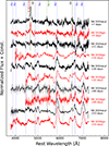 |
Fig. 12. Comparisons of the spectra of SN 2024acyl with SN 2018gjx at multiple epochs. The SN 2024acyl spectra are in red; SN 2018gjx spectra are in black. Spectra with a low S/N were binned. The original (unbinned) spectra are displayed in lighter colours behind. All the phases marked in the figure are from the (approximate) explosion epoch. |
During the phases 15 ≲ t ≲ 40 days (see the fourth to seventh spectra in Fig. 12), broad lines begin to appear. In SN 2018gjx, the P-Cygni profiles of He I become broad and prominent, originating from the expanding opaque ejecta (Prentice et al. 2020). This indicates that the ejecta have extended beyond the CSM and the photosphere is currently located near the outer boundary of the ejecta. Additionally, features of Type IIb SNe, such as weak Hα absorption, are present in SN 2018gjx. However, we do not observe these features in SN 2024acyl during comparable phases. In the spectrum at +26 days from explosion, there are no prominent broad P Cygni profiles. This discrepancy may be attributed to differences in CSM properties. For SN 2024acyl, the CSM is optically thick (τ = ∫κρ dr ≳ 100), and MCSM is comparable to Mej. Consequently, the formation of a CDS obscures the spectroscopic features of the ejecta (Dessart et al. 2015, 2022). Furthermore, given that the radioactive power in SN 2024acyl is much weaker than that of SN 2018gjx, the luminosity of SN 2024acyl is likely dominated by CSM interaction. Unlike SN 2018gjx, SN 2024acyl exhibits strong signatures of CSM interaction throughout its evolution.
At t ≳ 40 days (see the eighth to tenth spectra in Fig. 12), broad emission lines of He I appear in the spectra of both SNe. This indicates that the photosphere is receding as the ejecta become optically thin (where τ ∝ t−2). Consequently, the interaction with the CSM becomes visible again, resulting in broad emission lines, a feature commonly observed in Type Ibn SNe. Furthermore, the spectra of both SN 2024acyl and SN 2018gjx display potential P Cygni absorption features associated with He Iλ5876. For SN 2024acyl, the velocity estimated from this possible P Cygni absorption is  , significantly higher than both the wind velocity and the initial CSM velocity (∼1000 km s−1). This suggests that the absorption profile originates from the expanding ejecta or the CDS. Since apparent absorption features can sometimes mimic dips in the pseudocontinuum caused by metal lines (e.g. Pastorello et al. 2015a; Kool et al. 2021), it is necessary to confirm that these features originate from optically thick ejecta. Following the method of Prentice et al. (2020), we estimate the velocity of the possible absorption feature of He Iλ6678. We measure a velocity of
  . This value is consistent with the estimate obtained from He Iλ5876, reinforcing the interpretation that these absorption features likely originate from the expanding ejecta and/or CDS. The profile of the He Iλ5876 broad emission line also shows a profile similar to that of SN 2018gjx, which is symmetric in the late phases, indicating that there was no prominent dust formation in SN 2024acyl similar to that in SN 2018gjx. Additionally, an asymmetric or toroidal CSM geometry (Smith et al. 2015; Prentice et al. 2020) may explain the visibility of these features, as ejecta signatures can remain observable through regions of lower optical depth.
Although there are several similarities between SN 2018gjx and SN 2024acyl, the relatively weak Hα emission line in the early phases and the strong signature of CSM interaction throughout its evolution make it difficult to classify SN 2024acyl as a Type IIb SN exploding in He-rich CSM. Compared to SN 2018gjx, SN 2024acyl is more likely an H-poor event. The signature of Hα in SN 2024acyl is weak in early phases compared with SN 2018gjx. In the late phases of SN 2024acyl, Hα gradually becomes prominent, but present as a pure narrow emission line without any P Cygni profile. This may be due to a small amount of residual hydrogen being excited during the late phases in an optically thin region, which is similar to most of the SNe Ibn such as SN 2006jc and SN 2020bqj. The discrepancy of CSM interaction strength can be explained either by inherently strong interaction, as previously discussed, or by a toroidal CSM geometry viewed edge-on. Also, since the case for a WR star as the progenitor of SN 2024acyl is less favoured in the previous discussion, it is also difficult to explain the progenitor of SN 2024acyl within the framework of a Type IIb event. Although these features of SN 2024acyl share similar physical mechanisms with SN 2018gjx, they are inconsistent with an SN IIb classification.
5.3. A possible low-mass progenitor
An alternative scenario for SN 2024acyl is to invoke the explosion of a low-mass (MpreSN ≲ 3.5 M⊙; Woosley 2019; Dessart et al. 2022) He star within a binary system, resulting in a partially stripped CC SN. This binary channel allows the progenitor to be of lower mass, stripped of its H envelope through binary interaction, rather than due to mass loss in a very massive progenitor. As an extreme example, Sanders et al. (2013) explored a white dwarf in a helium-rich CSM within a binary system as a possible progenitor channel for PS1-12sk. This scenario does not require a massive progenitor and recent star formation. The derived parameters of SN 2024acyl seem to well match those of PS1-12sk, such as the low explosion energy (Ekin(SN 2024acyl) =  erg; Ekin(PS1-12sk) ≈1050 erg), the small ejecta mass (Mej(SN 2024acyl) =
  ; Mej(PS1-12sk) ≈0.3 M⊙), along with the presence of H features in the spectra. The MNi of SN 2024acyl is lower than that of other Type Ibn SNe (which average ∼0.04 M⊙; Maeda & Moriya 2022) and is comparable to values for low-mass Type IIP SNe (Elmhamdi et al. 2003), suggesting that SN 2024acyl likely originated from a low-mass progenitor. In addition, SN 2024acyl is located at the edge of the host galaxy, ∼34 kpc from its centre, suggesting a potential lower star-formation rate in the nearby area, where it is less likely to form a massive WR-like progenitor (Hosseinzadeh et al. 2019; Warwick et al. 2025). The similarities with PS1-12sk suggest the progenitor of SN 2024acyl is likely a low-mass star, which might even be a helium white dwarf as proposed by Wang et al. (2024a) for a possible progenitor case of another low-mass event, SN 2020nxt. Furthermore, the overall photometric and spectroscopic observables of SN 2024acyl, along with their corresponding modelling results, can be naturally explained by the explosion of a low-mass He star progenitor.
From a spectroscopic point of view, as discussed in Sec. 4.5, the non-local thermodynamic equilibrium fits reproduce the main features and favour a low-mass helium-star progenitor – in particular, a model with a He-ZAMS mass of 4 M⊙, corresponding to a pre-SN mass of 3.16 M⊙. Building on the interaction-powered framework, the spectra of SN 2024acyl are consistent with emission from a compact CDS formed by the collision of low-mass ejecta with a slowly expanding, He-rich circumstellar shell. In such models, the radiative output is dominated by shock power and non-thermal deposition, with radioactive heating contributing little at the epochs studied (Dessart et al. 2022). The persistence of strong He I lines, accompanied by weak Balmer features, implies a confined, helium-dominated CSM. These constraints support a low-mass helium-star progenitor, likely stripped via binary interaction, rather than a very massive WR star. From a photometric point of view (see Sec. 3.3), the low posteriors of Mej and Ek suggest SN 2024acyl was a slightly underenergetic event with a small ejected mass. In a single-star scenario, the stellar winds from a moderate-mass progenitor are too weak to effectively strip its hydrogen envelope. However, in a close binary system, the progenitor can be stripped through mass transfer to a companion star (Podsiadlowski et al. 1992).
Finally, we compared the bolometric light curve of SN 2024acyl with a selection of radiation-hydrodynamics models from Dessart et al. (2022) in Fig. 13. The bolometric light curve of SN 2024acyl was constructed by fitting black-body models to the SED using an a Markov chain Monte Carlo method, with uncertainties quantified by the 68% confidence intervals of the posterior distributions. We focused on their simulations of an explosion interacting with a dense, shell-like CSM. These models simulate a low-energy explosion (Ek = 7.5 × 1049 erg) colliding with a 1.0 M⊙ CSM shell. The primary comparison is between a high-mass ejecta scenario (models E1 and E2, with Mej = 1.49 M⊙) and a low-mass ejecta scenario (models E5 and E6, with Mej = 0.15 M⊙). Within these pairs, the models further differ in the expansion velocity of the CSM, corresponding to CSM kinetic energies of 1047 erg and 1049 erg, respectively. The observed light-curve profile of SN 2024acyl shows a strong resemblance to the low-mass ejecta models (E5 and E6) rather than high-mass ejecta models (E1 and E2). This result suggests that the event was likely produced by an explosion with a small ejecta mass and low kinetic energy, consistent with the light-curve fitting result in Sec. 3.3. Thus, if we have such a small ejecta mass and low kinetic energy, the straightforward interpretation would more likely be that SN 2024acyl was a low-mass stripped helium star.
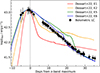 |
Fig. 13. Bolometric light curve of SN 2024acyl compared with several selected interaction models from Dessart et al. (2022). The comparison interaction configurations are overplotted and normalised to the peak luminosity of SN 2024acyl. |
Furthermore, in the required binary-star scenario, the strong and eruptive mass loss responsible for the dense and shell-like CSM is attributed to late-stage instabilities. Mechanisms such as unstable mass transfer or a nuclear flash can eject a dense, shell-like, helium-rich CSM in the final years before the explosion (Wang et al. 2024a). This scenario is consistent with our observations, as radiative-hydrodynamics models assuming such a shell-like geometry successfully reproduce the key features of the bolometric light curve of SN 2024acyl.
6. Conclusions
In this paper, we have presented observations of the recent, well-monitored Type Ibn SN 2024acyl, which has a relatively faint luminosity, linearly and rapidly evolving light curves, and flash-ionisation spectroscopic features. We propose that SN 2024acyl is likely the interaction-powered explosion of a low-mass He star that evolved in an interacting binary, and the CSM with some residual H may have been produced by a mass-transfer process of the binary system. This is based on the observational properties of SN 2024acyl, the multi-band light-curve modelling with MOSFiT, bolometric light curve and spectral comparisons with theoretical models, and a comparison with other SNe Ibn with similar photometric and spectroscopic features. However, a late-type WR star with hydrogen or even an Ofpe/WN9 star with fallback accretion cannot be entirely ruled out. Lacking a direct detection for the pre-SN mass loss of the progenitor of SN 2024acyl and its companion star, a robust conclusion about the progenitor star, whether arising from a high-mass WR star, a lower-mass He star, or even a He white dwarf in a binary system, cannot be made.
Advanced observational facilities, such as the Mephisto15 and the Vera C. Rubin Observatory16, will help increase the discovery rate and may trace the progenitor activities of Type Ibn events. New spectroscopic instrumentation such as SOXS (Son Of X-Shooter; see Radhakrishnan Santhakumari et al. 2024), installed on the NTT at the La Silla Observatory in Chile, will play a key role in classifying and following up these transients. In addition, the Chinese Space Station Telescope17 will enhance our ability to detect and characterise the progenitors of such events. The endeavours we undertake in both theoretical models and advanced facilities will be beneficial to enhancing our understanding of the nature of the poorly understood Type Ibn SNe.
Data availability
Ultraviolet and optical photometric measurements of SN 2024acyl are available at the CDS via https://cdsarc.cds.unistra.fr/viz-bin/cat/J/A+A/707/A157. Our observations of the spectra are available via the Weizmann Interactive SN Data Repository (WISeREP; Yaron & Gal-Yam 2012).
Acknowledgments
We are grateful to the anonymous referee for insightful comments and suggestions that improved the paper. We thank Luc Dessart for kindly providing the spectral models for this Type Ibn SN. This work is supported by the National Key Research and Development Program of China (grants 2024YFA1611603, 2021YFA1600404), the National Natural Science Foundation of China (grants 12303054, 12225304, 12288102, 12373038), the Yunnan Fundamental Research Projects (grants 202401AU070063, 202501AS070078), the Yunnan Revitalization Talent Support Program (Yunling Scholar Project and Innovation Team Project), the Yunnan Science and Technology Program (grants 202501AS070005, 202201BC070003), the International Centre of Supernovae, Yunnan Key Laboratory (grant 202302AN360001), the Natural Science Foundation of Xinjiang Uygur Autonomous Region (grant 2024D01D32), and the Tianshan Talent Training Program (grant 2023TSYCLJ0053). A.P., A.R., S.B., E.C., N.E.R., and G.V. acknowledge support from the PRIN-INAF 2022, “Shedding light on the nature of gap transients: from the observations to the models.” A.R. was also supported by the GRAWITA Large Program Grant (PI P. D’Avanzo). E.C. acknowledges support from MIUR, PRIN 2020 (METE, grant 2020KB33TP). K.M. was supported by Japan Society for the Promotion of Science (JSPS) KAKENHI grants JP24KK0070 and JP24H01810, and by JSPS bilateral program JPJSBP120229923. B.K. is supported by the “Special Project for High-End Foreign Experts,” Xingdian Funding from Yunnan Province. T.-W.C. acknowledges financial support from the Yushan Fellow Program by the Ministry of Education, Taiwan (MOE-111-YSFMS-0008-001-P1) and the National Science and Technology Council, Taiwan (NSTC grant 114-2112-M-008-021-MY3). N.E.R. acknowledges support from the Spanish Ministerio de Ciencia e Innovación (MCIN) and the Agencia Estatal de Investigación (AEI) 10.13039/501100011033 under the program Unidad de Excelencia María de Maeztu CEX2020-001058-M. C.P.G. acknowledges financial support from the Secretary of Universities and Research (Government of Catalonia) and by the Horizon 2020 Research and Innovation Programme of the European Union under the Marie Skłodowska-Curie and the Beatriu de Pinós 2021 BP 00168 programme. Both C.P.G. and M.G.B. were supported by the Spanish Ministerio de Ciencia e Innovación (MCIN) and the Agencia Estatal de Investigación (AEI; 10.13039/501100011033) under the PID2023-151307NB-I00 SNNEXT project, by the Centro Superior de Investigaciones Científicas (CSIC) under the PIE project 20215AT016 and the programme Unidad de Excelencia María de Maeztu CEX2020-001058-M, and by the Departament de Recerca i Universitats de la Generalitat de Catalunya through the 2021-SGR-01270 grant. T.K. acknowledges support from the Research Council of Finland project 360274. S. Mattila acknowledges financial support from the Research Council of Finland project 350458. S. Moran is funded by Leverhulme Trust grant RPG-2023-240. M.D. Stritzinger is funded by the Independent Research Fund Denmark (IRFD, grant number 10.46540/2032-00022B). T.E.M.B. is funded by Horizon Europe ERC grant no. 101125877. T.P. acknowledges financial support from the Slovenian Research Agency (grants I0-0033, P1-0031, J1-2460 and N1-0344). H.K. was funded by the Research Council of Finland projects 324504, 328898, and 353019. A.F. acknowledges funding by the European Union – NextGenerationEU RFF M4C2 1.1 PRIN 2022 project “2022RJLWHN URKA” and by INAF 2023 Theory Grant ObFu 1.05.23.06.06 “Understanding R-process & Kilonovae Aspects (URKA).” J.Z. is supported by the National Key R&D Program of China with No. 2021YFA1600404, the National Natural Science Foundation of China (12173082, 12333008), the Yunnan Fundamental Research Projects (grants 202401BC070007 and 202201AT070069), the Top-notch Young Talents Program of Yunnan Province, the Light of West China Program provided by the Chinese Academy of Sciences, and the International Centre of Supernovae, Yunnan Key Laboratory (grant 202302AN360001). X.F.W. is supported by the National Natural Science Foundation of China (grants 12288102, 12033003, and 11633002) and the Tencent Xplorer Prize. A.V.F.’s research group at U.C. Berkeley acknowledges financial assistance from the Christopher R. Redlich Fund, as well as donations from Gary and Cynthia Bengier, Clark and Sharon Winslow, Alan Eustace and Kathy Kwan, William Draper, Timothy and Melissa Draper, Briggs and Kathleen Wood, Sanford Robertson (W.Z. is a Bengier-Winslow-Eustace Specialist in Astronomy, T.G.B. is a Draper-Wood-Robertson Specialist in Astronomy), and numerous other donors. We acknowledge the support of the staffs of the various observatories at which data were obtained. The observations were in part carried out within the framework of Subaru-Gemini time exchange program (under the project S24B-041 / GN-2024B-Q-101: PI, K. Maeda) which is operated by the National Astronomical Observatory of Japan. We are honored and grateful for the opportunity of observing the Universe from Maunakea, which has the cultural, historical and natural significance in Hawaii. Funding for the LJT has been provided by the CAS and the People’s Government of Yunnan Province. The LJT is jointly operated and administrated by YNAO and the Center for Astronomical Mega-Science, CAS. Based in part on observations made with the Nordic Optical Telescope, owned in collaboration by the University of Turku and Aarhus University, and operated jointly by Aarhus University, the University of Turku, and the University of Oslo, representing Denmark, Finland, and Norway, the University of Iceland, and Stockholm University at the Observatorio del Roque de los Muchachos, La Palma, Spain, of the Instituto de Astrofisica de Canarias. Observations from the NOT were obtained through the NUTS2 collaboration which is supported in part by the Instrument Centre for Danish Astrophysics (IDA), and the Finnish Centre for Astronomy with ESO (FINCA) via Academy of Finland grant nr 306531. The data presented here were obtained in part with ALFOSC, which is provided by the Instituto de Astrofisica de Andalucia (IAA) under a joint agreement with the University of Copenhagen and NOTSA. The Liverpool Telescope is operated on the island of La Palma by Liverpool John Moores University in the Spanish Observatorio del Roque de los Muchachos of the Instituto de Astrofisica de Canarias with financial support from the UK Science and Technology Facilities Council. The Italian Telescopio Nazionale Galileo (TNG) operated on the island of La Palma by the Fundación Galileo Galilei of the INAF (Istituto Nazionale di Astrofisica) at the Spanish Observatorio del Roque de los Muchachos of the Instituto de Astrofísica de Canarias. This article is also based on observations made in the Observatorios de Canarias del IAC with the Telescopio Nazionale Galileo, operated on the island of La Palma by INAF at the Observatorio del Roque de los Muchachos under the program A50TAC_41 (PI: G. Valerin). Based in part on observations collected at Copernico and Schmidt telescopes (Asiago Mount Ekar, Italy) of the INAF – Osservatorio Astronomico di Padova. The Chinese Tsinghua–Nanshan Optical Telescope (TNOT) operated at Nanshan Station by Xinjiang Astronomical Observatory of the Chinese Academy of Sciences, located in Xinjiang, China. Based in part on observations collected with the 0.8 m TNOT equipped with an Andor camera at Nanshan Station of Xinjiang Astronomical Observatory. Mephisto is developed at and operated by the South-Western Institute for Astronomy Research of Yunnan University (SWIFAR-YNU), funded by the “Yunnan University Development Plan for World-Class University” and “Yunnan University Development Plan for World-Class Astronomy Discipline.” Based on the “Key Laboratory of Survey Science of Yunnan Province” with project No. 202449CE340002. Based in part on observations collected at the European Organisation for Astronomical Research in the Southern Hemisphere, Chile, as part of ePESSTO+ (the advanced Public ESO Spectroscopic Survey for Transient Objects Survey – PI: Inserra). ePESSTO+ observations were obtained under ESO program ID 112.25JQ. A major upgrade of the Kast spectrograph on the Shane 3 m telescope at Lick Observatory, led by Brad Holden, was made possible through generous gifts from the Heising-Simons Foundation, William and Marina Kast, and the University of California Observatories. Research at Lick Observatory is partially supported by a generous gift from Google. This work has made use of data from the Asteroid Terrestrial-impact Last Alert System (ATLAS) project. The Asteroid Terrestrial-impact Last Alert System (ATLAS) project is primarily funded to search for near-Earth objects (NEOs) through National Aeronautics and Space Administration (NASA) grants NN12AR55G, 80NSSC18K0284, and 80NSSC18K1575; byproducts of the NEO search include images and catalogs from the survey area. This work was partially funded by Kepler/K2 grant J1944/80NSSC19K0112 and HST GO-15889, and STFC grants ST/T000198/1 and ST/S006109/1. The ATLAS science products have been made possible through the contributions of the University of Hawaii Institute for Astronomy, the Queen’s University Belfast, the Space Telescope Science Institute, the South African Astronomical Observatory, and The Millennium Institute of Astrophysics (MAS), Chile. Pan-STARRS is a project of the Institute for Astronomy of the University of Hawaii, and is supported by the NASA SSO Near Earth Observation Program under grants 80NSSC18K0971, NNX14AM74G, NNX12AR65G, NNX13AQ47G, NNX08AR22G, 80NSSC21K1572 and by the State of Hawaii. The Pan-STARRS1 Surveys (PS1) and the PS1 public science archive have been made possible through contributions by the Institute for Astronomy, the University of Hawaii, the Pan-STARRS Project Office, the Max-Planck Society and its participating institutes, the Max Planck Institute for Astronomy, Heidelberg and the Max Planck Institute for Extraterrestrial Physics, Garching, The Johns Hopkins University, Durham University, the University of Edinburgh, the Queen’s University Belfast, the Harvard-Smithsonian Center for Astrophysics, the Las Cumbres Observatory Global Telescope Network Incorporated, the National Central University of Taiwan, STScI, NASA under grant NNX08AR22G issued through the Planetary Science Division of the NASA Science Mission Directorate, NSF grant AST-1238877, the University of Maryland, Eotvos Lorand University (ELTE), the Los Alamos National Laboratory, and the Gordon and Betty Moore Foundation. We acknowledge the use of public data from the Swift data archive. SDSS is managed by the Astrophysical Research Consortium for the Participating Institutions of the SDSS Collaboration including the Brazilian Participation Group, the Carnegie Institution for Science, Carnegie Mellon University, Center for Astrophysics | Harvard & Smithsonian (CfA), the Chilean Participation Group, the French Participation Group, Instituto de Astrofísica de Canarias, The Johns Hopkins University, Kavli Institute for the Physics and Mathematics of the Universe (IPMU) / University of Tokyo, the Korean Participation Group, Lawrence Berkeley National Laboratory, Leibniz Institut für Astrophysik Potsdam (AIP), Max-Planck-Institut für Astronomie (MPIA Heidelberg), Max-Planck-Institut für Astrophysik (MPA Garching), Max-Planck-Institut für Extraterrestrische Physik (MPE), National Astronomical Observatories of China, New Mexico State University, New York University, University of Notre Dame, Observatório Nacional / MCTI, The Ohio State University, Pennsylvania State University, Shanghai Astronomical Observatory, United Kingdom Participation Group, Universidad Nacional Autónoma de México, University of Arizona, University of Colorado Boulder, University of Oxford, University of Portsmouth, University of Utah, University of Virginia, University of Washington, University of Wisconsin, Vanderbilt University, and Yale University. This research has made use of the NASA/IPAC Extragalactic Database (NED), which is operated by the Jet Propulsion Laboratory, California Institute of Technology, under contract with NASA.
References
- Anupama, G. C., Sahu, D. K., Gurugubelli, U. K., et al. 2009, MNRAS, 392, 894 [NASA ADS] [CrossRef] [Google Scholar]
- Arnett, W. D. 1982, ApJ, 253, 785 [Google Scholar]
- Ben-Ami, T., Arcavi, I., Newsome, M., et al. 2023, ApJ, 946, 30 [NASA ADS] [CrossRef] [Google Scholar]
- Bianchi, L., Bohlin, R., & Massey, P. 2004, ApJ, 601, 228 [Google Scholar]
- Blinnikov, S., Chugai, N., Lundqvist, P., et al. 2003, in From Twilight to Highlight: The Physics of Supernovae, eds. W. Hillebrandt, & B. Leibundgut, 23 [Google Scholar]
- Bostroem, K. A., Pearson, J., Shrestha, M., et al. 2023, ApJ, 956, L5 [NASA ADS] [CrossRef] [Google Scholar]
- Brown, T. M., Baliber, N., Bianco, F. B., et al. 2013, PASP, 125, 1031 [Google Scholar]
- Bruch, R. J., Gal-Yam, A., Yaron, O., et al. 2023, ApJ, 952, 119 [NASA ADS] [CrossRef] [Google Scholar]
- Buzzoni, B., Delabre, B., Dekker, H., et al. 1984, The Messenger, 38, 9 [NASA ADS] [Google Scholar]
- Cai, Y. Z., Pastorello, A., Fraser, M., et al. 2018, MNRAS, 480, 3424 [NASA ADS] [Google Scholar]
- Chambers, K. C., Magnier, E. A., Metcalfe, N., et al. 2016, ArXiv e-prints [arXiv:1612.05560] [Google Scholar]
- Chatzopoulos, E., Wheeler, J. C., & Vinko, J. 2012, ApJ, 746, 121 [Google Scholar]
- Chen, X., Kumar, B., Er, X., et al. 2024, ApJ, 971, L2 [Google Scholar]
- Chevalier, R. A. 1982, ApJ, 258, 790 [NASA ADS] [CrossRef] [Google Scholar]
- Chevalier, R. A., & Fransson, C. 2006, ApJ, 651, 381 [NASA ADS] [CrossRef] [Google Scholar]
- Conti, P. S. 1975, Memoires of the Societe Royale des Sciences de Liege, 9, 193 [Google Scholar]
- Dessart, L. 2024, ArXiv e-prints [arXiv:2405.04259] [Google Scholar]
- Dessart, L., Audit, E., & Hillier, D. J. 2015, MNRAS, 449, 4304 [Google Scholar]
- Dessart, L., Hillier, D. J., & Kuncarayakti, H. 2022, A&A, 658, A130 [NASA ADS] [CrossRef] [EDP Sciences] [Google Scholar]
- Di Carlo, E., Corsi, C., Arkharov, A. A., et al. 2008, ApJ, 684, 471 [NASA ADS] [CrossRef] [Google Scholar]
- Djupvik, A. A., & Andersen, J. 2010, Astrophys. Space Sci. Proc., 14, 211 [NASA ADS] [CrossRef] [Google Scholar]
- Dong, Y., Villar, V. A., Nugent, A., et al. 2025, ArXiv e-prints [arXiv:2511.03926] [Google Scholar]
- Elmhamdi, A., Chugai, N. N., & Danziger, I. J. 2003, A&A, 404, 1077 [NASA ADS] [CrossRef] [EDP Sciences] [Google Scholar]
- Farias, D., Gall, C., Narayan, G., et al. 2024, ApJ, 977, 152 [Google Scholar]
- Farias, D., Gall, C., Villar, V. A., et al. 2025, Characterization of type Ibn SNe [Google Scholar]
- Fassia, A., Meikle, W. P. S., Chugai, N., et al. 2001, MNRAS, 325, 907 [NASA ADS] [CrossRef] [Google Scholar]
- Filippenko, A. V. 1982, PASP, 94, 715 [Google Scholar]
- Filippenko, A. V. 1997, ARA&A, 35, 309 [NASA ADS] [CrossRef] [Google Scholar]
- Flewelling, H. A., Magnier, E. A., Chambers, K. C., et al. 2020, ApJS, 251, 7 [NASA ADS] [CrossRef] [Google Scholar]
- Foley, R. J., Smith, N., Ganeshalingam, M., et al. 2007, ApJ, 657, L105 [NASA ADS] [CrossRef] [Google Scholar]
- Fransson, C., Lundqvist, P., & Chevalier, R. A. 1996, ApJ, 461, 993 [NASA ADS] [CrossRef] [Google Scholar]
- Fraser, M. 2020, Royal Society Open Science, 7, 200467 [Google Scholar]
- Gal-Yam, A. 2017, Observational and Physical Classification of Supernovae (Springer International Publishing), 195 [Google Scholar]
- Gal-Yam, A., Arcavi, I., Ofek, E. O., et al. 2014, Nature, 509, 471 [CrossRef] [Google Scholar]
- Gangopadhyay, A., Misra, K., Hiramatsu, D., et al. 2020, ApJ, 889, 170 [NASA ADS] [CrossRef] [Google Scholar]
- Gangopadhyay, A., Misra, K., Hosseinzadeh, G., et al. 2022, ApJ, 930, 127 [NASA ADS] [CrossRef] [Google Scholar]
- Gangopadhyay, A., Dukiya, N., Moriya, T. J., et al. 2025, MNRAS, 537, 2898 [Google Scholar]
- Gimeno, G., Roth, K., Chiboucas, K., et al. 2016, SPIE Conf. Ser., 9908, 99082S [NASA ADS] [Google Scholar]
- Gorbikov, E., Gal-Yam, A., Ofek, E. O., et al. 2014, MNRAS, 443, 671 [NASA ADS] [CrossRef] [Google Scholar]
- Guillochon, J., Nicholl, M., Villar, V. A., et al. 2018, ApJS, 236, 6 [NASA ADS] [CrossRef] [Google Scholar]
- Hillier, D. J., & Dessart, L. 2012, MNRAS, 424, 252 [CrossRef] [Google Scholar]
- Hook, I. M., Jørgensen, I., Allington-Smith, J. R., et al. 2004, PASP, 116, 425 [NASA ADS] [CrossRef] [Google Scholar]
- Hosseinzadeh, G., Arcavi, I., Valenti, S., et al. 2017, ApJ, 836, 158 [Google Scholar]
- Hosseinzadeh, G., McCully, C., Zabludoff, A. I., et al. 2019, ApJ, 871, L9 [Google Scholar]
- Jacobson-Galán, W. V., Davis, K. W., Kilpatrick, C. D., et al. 2024, ApJ, 972, 177 [CrossRef] [Google Scholar]
- Karamehmetoglu, E., Taddia, F., Sollerman, J., et al. 2017, A&A, 602, A93 [NASA ADS] [CrossRef] [EDP Sciences] [Google Scholar]
- Khakpash, S., Bianco, F. B., Modjaz, M., et al. 2024, ApJS, 275, 37 [Google Scholar]
- Khazov, D., Yaron, O., Gal-Yam, A., et al. 2016, ApJ, 818, 3 [CrossRef] [Google Scholar]
- Kool, E. C., Karamehmetoglu, E., Sollerman, J., et al. 2021, A&A, 652, A136 [NASA ADS] [CrossRef] [EDP Sciences] [Google Scholar]
- Labrie, K., Simpson, C., Cardenes, R., et al. 2023, Res. Notes Am. Astron. Soc., 7, 214 [Google Scholar]
- Li, L.-H., Benetti, S., Cai, Y.-Z., et al. 2025, A&A, 704, A233 [NASA ADS] [CrossRef] [EDP Sciences] [Google Scholar]
- Maeda, K., & Moriya, T. J. 2022, ApJ, 927, 25 [NASA ADS] [CrossRef] [Google Scholar]
- Maeda, K., Tanaka, M., Nomoto, K., et al. 2007, ApJ, 666, 1069 [NASA ADS] [CrossRef] [Google Scholar]
- Magnier, E. A., Chambers, K. C., Flewelling, H. A., et al. 2020a, ApJS, 251, 3 [NASA ADS] [CrossRef] [Google Scholar]
- Magnier, E. A., Schlafly, E. F., Finkbeiner, D. P., et al. 2020b, ApJS, 251, 6 [NASA ADS] [CrossRef] [Google Scholar]
- Magnier, E. A., Sweeney, W. E., Chambers, K. C., et al. 2020c, ApJS, 251, 5 [NASA ADS] [CrossRef] [Google Scholar]
- Matheson, T., Filippenko, A. V., Chornock, R., Leonard, D. C., & Li, W. 2000, AJ, 119, 2303 [NASA ADS] [CrossRef] [Google Scholar]
- Mattila, S., Meikle, W. P. S., Lundqvist, P., et al. 2008, MNRAS, 389, 141 [NASA ADS] [CrossRef] [Google Scholar]
- Maund, J. R., Pastorello, A., Mattila, S., Itagaki, K., & Boles, T. 2016, ApJ, 833, 128 [NASA ADS] [CrossRef] [Google Scholar]
- Metzger, B. D. 2022, ApJ, 932, 84 [NASA ADS] [CrossRef] [Google Scholar]
- Miller, J. S., & Stone, R. P. S. 1993, Lick Obs. Tech. Rep. 66 (Santa Cruz: Lick Obs) [Google Scholar]
- Molinari, E., Conconi, P., & Pucillo, M. 1997, Mem. Soc. Astron. It., 68, 231 [NASA ADS] [Google Scholar]
- Moriya, T., Tominaga, N., Tanaka, M., et al. 2010, ApJ, 719, 1445 [NASA ADS] [CrossRef] [Google Scholar]
- Moriya, T. J., Müller, B., Blinnikov, S. I., et al. 2025, PASJ, 77, 1385 [Google Scholar]
- Nasa High Energy Astrophysics Science Archive Research Center (Heasarc) 2014, Astrophysics Source Code Library [record ascl:1408.004] [Google Scholar]
- Nicholl, M., Guillochon, J., & Berger, E. 2017, ApJ, 850, 55 [NASA ADS] [CrossRef] [Google Scholar]
- Nyholm, A., Sollerman, J., Taddia, F., et al. 2017, A&A, 605, A6 [NASA ADS] [CrossRef] [EDP Sciences] [Google Scholar]
- Pastorello, A., Smartt, S. J., Mattila, S., et al. 2007, Nature, 447, 829 [NASA ADS] [CrossRef] [Google Scholar]
- Pastorello, A., Mattila, S., Zampieri, L., et al. 2008a, MNRAS, 389, 113 [Google Scholar]
- Pastorello, A., Quimby, R. M., Smartt, S. J., et al. 2008b, MNRAS, 389, 131 [NASA ADS] [CrossRef] [Google Scholar]
- Pastorello, A., Benetti, S., Brown, P. J., et al. 2015a, MNRAS, 449, 1921 [Google Scholar]
- Pastorello, A., Prieto, J. L., Elias-Rosa, N., et al. 2015b, MNRAS, 453, 3649 [Google Scholar]
- Pastorello, A., Tartaglia, L., Elias-Rosa, N., et al. 2015c, MNRAS, 454, 4293 [Google Scholar]
- Pastorello, A., Wyrzykowski, Ł., Valenti, S., et al. 2015d, MNRAS, 449, 1941 [NASA ADS] [CrossRef] [Google Scholar]
- Pastorello, A., Wang, X. F., Ciabattari, F., et al. 2016, MNRAS, 456, 853 [Google Scholar]
- Pastorello, A., Reguitti, A., Tartaglia, L., et al. 2025, A&A, 701, A32 [NASA ADS] [CrossRef] [EDP Sciences] [Google Scholar]
- Pellegrino, C., Howell, D. A., Vinkó, J., et al. 2022, ApJ, 926, 125 [NASA ADS] [CrossRef] [Google Scholar]
- Pellegrino, C., Modjaz, M., Takei, Y., et al. 2024, ApJ, 977, 2 [Google Scholar]
- Podsiadlowski, P., Joss, P. C., & Hsu, J. J. L. 1992, ApJ, 391, 246 [Google Scholar]
- Prentice, S. J., Ashall, C., James, P. A., et al. 2019, MNRAS, 485, 1559 [NASA ADS] [CrossRef] [Google Scholar]
- Prentice, S. J., Maguire, K., Boian, I., et al. 2020, MNRAS, 499, 1450 [CrossRef] [Google Scholar]
- Pursiainen, M., Leloudas, G., Schulze, S., et al. 2023, ApJ, 959, L10 [NASA ADS] [CrossRef] [Google Scholar]
- Radhakrishnan Santhakumari, K. K., Battaini, F., Di Filippo, S., et al. 2024, ArXiv e-prints [arXiv:2407.17288] [Google Scholar]
- Reguitti, A., Pastorello, A., Pignata, G., et al. 2022, A&A, 662, L10 [NASA ADS] [CrossRef] [EDP Sciences] [Google Scholar]
- Roming, P. W. A., Kennedy, T. E., Mason, K. O., et al. 2005, Space Sci. Rev., 120, 95 [Google Scholar]
- Sanders, N. E., Soderberg, A. M., Foley, R. J., et al. 2013, ApJ, 769, 39 [Google Scholar]
- Santos, R., Duarte, J., Ghendrih, M., et al. 2024, Transient Name Server Classification Report, 2024–4787, 1 [Google Scholar]
- Schlafly, E. F., & Finkbeiner, D. P. 2011, ApJ, 737, 103 [Google Scholar]
- Schlegel, E. M. 1990, MNRAS, 244, 269 [NASA ADS] [Google Scholar]
- Shingles, L., Smith, K. W., Young, D. R., et al. 2021, Transient Name Server AstroNote, 7, 1 [NASA ADS] [Google Scholar]
- Shivvers, I., Groh, J. H., Mauerhan, J. C., et al. 2015, ApJ, 806, 213 [NASA ADS] [CrossRef] [Google Scholar]
- Silverman, J. M., Foley, R. J., Filippenko, A. V., et al. 2012, MNRAS, 425, 1789 [Google Scholar]
- Smartt, S. J., Valenti, S., Fraser, M., et al. 2015, A&A, 579, A40 [NASA ADS] [CrossRef] [EDP Sciences] [Google Scholar]
- Smith, K. W., Smartt, S. J., Young, D. R., et al. 2020, PASP, 132, 085002 [Google Scholar]
- Smith, N. 2017, Interacting Supernovae: Types IIn and Ibn (Cham: Springer International Publishing), 403 [Google Scholar]
- Smith, N., Foley, R. J., & Filippenko, A. V. 2008, ApJ, 680, 568 [Google Scholar]
- Smith, N., Mauerhan, J. C., Silverman, J. M., et al. 2012, MNRAS, 426, 1905 [NASA ADS] [CrossRef] [Google Scholar]
- Smith, N., Mauerhan, J. C., Cenko, S. B., et al. 2015, MNRAS, 449, 1876 [Google Scholar]
- Soubrouillard, E., & Leadbeater, R. 2024, Transient Name Server Classification Report, 2024–4856, 1 [Google Scholar]
- Speagle, J. S. 2020, MNRAS, 493, 3132 [Google Scholar]
- Spergel, D. N., Bean, R., Doré, O., et al. 2007, ApJS, 170, 377 [NASA ADS] [CrossRef] [Google Scholar]
- Springob, C. M., Haynes, M. P., Giovanelli, R., & Kent, B. R. 2005, ApJS, 160, 149 [NASA ADS] [CrossRef] [Google Scholar]
- Steele, I. A., Smith, R. J., Rees, P. C., et al. 2004, SPIE Conf. Ser., 5489, 679 [Google Scholar]
- Stritzinger, M., Taddia, F., Fransson, C., et al. 2012, ApJ, 756, 173 [NASA ADS] [CrossRef] [Google Scholar]
- Sun, N.-C., Maund, J. R., Hirai, R., Crowther, P. A., & Podsiadlowski, P. 2020, MNRAS, 491, 6000 [NASA ADS] [CrossRef] [Google Scholar]
- Taddia, F., Sollerman, J., Fremling, C., et al. 2015, A&A, 580, A131 [NASA ADS] [CrossRef] [EDP Sciences] [Google Scholar]
- Tominaga, N., Limongi, M., Suzuki, T., et al. 2008, ApJ, 687, 1208 [NASA ADS] [CrossRef] [Google Scholar]
- Tonry, J. L., Denneau, L., Heinze, A. N., et al. 2018, PASP, 130, 064505 [Google Scholar]
- Tonry, J., Denneau, L., Weiland, H., et al. 2024, Transient Name Server Discovery Report, 2024–4707, 1 [Google Scholar]
- Tsuna, D., Wu, S. C., Fuller, J., Dong, Y., & Piro, A. L. 2024, Open J. Astrophys., 7, 82 [Google Scholar]
- Turatto, M., Cappellaro, E., Danziger, I. J., et al. 1993, MNRAS, 262, 128 [CrossRef] [Google Scholar]
- Valenti, S., Benetti, S., Cappellaro, E., et al. 2008, MNRAS, 383, 1485 [Google Scholar]
- Valenti, S., Pastorello, A., Cappellaro, E., et al. 2009, Nature, 459, 674 [NASA ADS] [CrossRef] [Google Scholar]
- Vallely, P. J., Prieto, J. L., Stanek, K. Z., et al. 2018, MNRAS, 475, 2344 [NASA ADS] [CrossRef] [Google Scholar]
- Villar, V. A., Berger, E., Metzger, B. D., & Guillochon, J. 2017, ApJ, 849, 70 [NASA ADS] [CrossRef] [Google Scholar]
- Walborn, N. R. 1977, ApJ, 215, 53 [NASA ADS] [CrossRef] [Google Scholar]
- Walborn, N. R. 1982, ApJ, 256, 452 [NASA ADS] [CrossRef] [Google Scholar]
- Wang, S.-Q., & Li, L. 2020, ApJ, 900, 83 [Google Scholar]
- Wang, C.-J., Bai, J.-M., Fan, Y.-F., et al. 2019, Res. Astron. Astrophys., 19, 149 [CrossRef] [Google Scholar]
- Wang, G.-J., Li, S.-Y., & Xia, J.-Q. 2020a, ApJS, 249, 25 [NASA ADS] [CrossRef] [Google Scholar]
- Wang, G.-J., Ma, X.-J., Li, S.-Y., & Xia, J.-Q. 2020b, ApJS, 246, 13 [NASA ADS] [CrossRef] [Google Scholar]
- Wang, G.-J., Ma, X.-J., & Xia, J.-Q. 2021a, MNRAS, 501, 5714 [NASA ADS] [Google Scholar]
- Wang, X., Lin, W., Zhang, J., et al. 2021b, ApJ, 917, 97 [NASA ADS] [CrossRef] [Google Scholar]
- Wang, Q., Goel, A., Dessart, L., et al. 2024a, MNRAS, 530, 3906 [NASA ADS] [CrossRef] [Google Scholar]
- Wang, Z. Y., Pastorello, A., Maeda, K., et al. 2024b, A&A, 691, A156 [NASA ADS] [CrossRef] [EDP Sciences] [Google Scholar]
- Wang, Z. Y., Pastorello, A., Cai, Y. Z., et al. 2025, A&A, 700, A156 [NASA ADS] [CrossRef] [EDP Sciences] [Google Scholar]
- Warwick, B., Lyman, J., Pursiainen, M., et al. 2025, MNRAS, 536, 3588 [Google Scholar]
- Waters, C. Z., Magnier, E. A., Price, P. A., et al. 2020, ApJS, 251, 4 [NASA ADS] [CrossRef] [Google Scholar]
- Woosley, S. E. 2019, ApJ, 878, 49 [Google Scholar]
- Woosley, S. E., & Weaver, T. A. 1995, ApJS, 101, 181 [Google Scholar]
- Wu, S. C., & Fuller, J. 2022, ApJ, 940, L27 [NASA ADS] [CrossRef] [Google Scholar]
- Yang, Y.-P., Liu, X., Pan, Y., et al. 2024, ApJ, 969, 126 [Google Scholar]
- Yaron, O., & Gal-Yam, A. 2012, PASP, 124, 668 [Google Scholar]
- Yaron, O., Perley, D. A., Gal-Yam, A., et al. 2017, Nat. Phys., 13, 510 [NASA ADS] [CrossRef] [Google Scholar]
- Yuan, X., Li, Z., Liu, X., et al. 2020, SPIE Conf. Ser., 11445, 114457M [Google Scholar]
- Zampieri, L., Shapiro, S. L., & Colpi, M. 1998, ApJ, 502, L149 [NASA ADS] [CrossRef] [Google Scholar]
- Zhang, J., Dessart, L., Wang, X., et al. 2024, ApJ, 970, L18 [NASA ADS] [CrossRef] [Google Scholar]
- Zhang, J., Lin, H., Wang, X., et al. 2023, Sci. Bull., 68, 2548 [NASA ADS] [CrossRef] [Google Scholar]
- Zou, X., Kumar, B., Teja, R. S., et al. 2026, ApJ, 997, 77 [Google Scholar]
ecsnoopy is a package for SN photometry using PSF fitting and/or template subtraction developed by E. Cappellaro. A package description can be found at https://sngroup.oapd.inaf.it/ecsnoopy.html
The comparison SNe Ibn include SNe 2006jc (Pastorello et al. 2007), 2010al (Pastorello et al. 2015a), 2019kbj (Ben-Ami et al. 2023), and 2019cj (Wang et al. 2024b).
Since the light curve is not sensitive to the density-profile parameters (n, δ), and the parameter s has only a minor effect on the light-curve shape, in Fig. 6 we present only a single best-fit scenario with n = 10, δ = 0, and s = 0.
Since we added the additional jitter term log(σ), it explicitly accounts for the underestimated systematic errors and intrinsic deviations from the model statistically.
The Ofpe/WN9 stars, also known as ‘slash stars’, were introduced by Walborn (1977, 1982) These objects are characterised by the presence of strong low-ionisation emission features (N II, He I) along with the normal high-ionisation Of-features (N III, He II) in their spectra. They exhibit spectroscopic properties that are intermediate between those of Of and WN stars, indicating that they are transition objects between Of and WR stars (e.g. Conti 1975; Bianchi et al. 2004).
Appendix A: Observational facilities used in the follow-up photometry of SN 2024acyl
Information on the instrumental setups.
Appendix B: Best-fit light-curve model for SN 2024acyl and comparisons
MOSFiT multi-band light-curve fitting results of SN 2024acyl with RD+CSI model. The parameters are converted to linear space.
Appendix C: Log of spectroscopic observations
Log of the spectroscopic observations of SN 2024acyl.
Appendix D: MOSFiT corner plots of SN 2024acyl
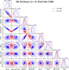 |
Fig. D.1. Corner plots showing the posterior distributions of the estimated parameters for SN 2024acyl, based on the Ni+CSM model using MOSFiT. All the models adopted the CSM density profile s = 0 (shell-like CSM). The blue region represents outer ejecta density profile n = 10 while red region represents n = 12. Median values are marked by dashed vertical lines, with the shaded regions representing the 68% confidence intervals. |
All Tables
Decline rates of the multi-band light curves of SN 2024acyl, along with their uncertainties, in units of mag (100 d)−1.
MOSFiT multi-band light-curve fitting results of SN 2024acyl with RD+CSI model. The parameters are converted to linear space.
All Figures
|
Fig. 1. SN 2024acyl in a NOT+ALFOSC coloured image taken with Johnson B, V, and Sloan r band filters on 2025 January 6. The SN is marked at the crosshair, near the centre of the image. |
| In the text | |
|
Fig. 2. Ultraviolet and optical light curves of SN 2024acyl. The dashed vertical line indicates the time of the o-band maximum light as the reference epoch. The vertical red lines at the top mark spectral observational epochs. The upper limits are plotted with empty symbols with arrows. The light curves for different filters are shifted with arbitrary constants, reported in the legend. The Mephisto u- and v-band data points in its unique filter system (for details see Chen et al. 2024; Yang et al. 2024) are indicated by uM and vM in the legend. Magnitude errors are usually smaller than the symbol size. |
| In the text | |
|
Fig. 3. Colour evolution of SN 2024acyl compared with the prototypical Type Ibn SN 2006jc and other fast, linearly declining SNe Ibn. Top panel: B − V colours. Bottom panel: R − I or r − i colours. The colour curves have been corrected for galactic extinction. |
| In the text | |
|
Fig. 4. Light curves in the V-band of SN 2024acyl, including the comparison SNe Ibn. Template V-band light curves for Type Ibn SNe are from Hosseinzadeh et al. (2017, blue) and Khakpash et al. (2024, green). Due to data-coverage limitations, SN 2023utc is represented using r-band photometry converted to the Vega system. |
| In the text | |
|
Fig. 5. Pseudobolometric light curves of SN 2024acyl and the comparison SNe Ibn. The comparison objects have luminosities comparable to that of the ‘optical’ luminosity of SN 2024acyl, integrating from the B to the I/i bands. |
| In the text | |
|
Fig. 6. Fits to the multi-band light curves of SN 2024acyl with n = 10, δ = 0, and s = 0 using the MOSFiT Monte Carlo code with the hybrid Ni+CSM model. For each filter, a subset of randomly sampled model light curves from the posterior distributions are displayed to illustrate the uncertainty of the model fits. |
| In the text | |
|
Fig. 7. Time sequence of SN 2024acyl spectra. Some prominent features, such as He I, He II, and N III, are marked with vertical lines, while the strongest telluric absorption bands are indicated with the ⊕ symbols. The phases reported to the right of each spectrum are from the epoch of o-band maximum light (MJD = 60652.49 ± 0.26; 2024-12-08). Spectra with a low S/N were binned with 20 Å each bin; the original (unbinned) spectra are displayed in lighter colours behind. Reddening and redshift corrections have been applied to the spectra. |
| In the text | |
|
Fig. 8. Temporal evolution of the He Iλ5876 line. Left panel: line-profile evolution in the velocity space. The dashed vertical line marking marks the rest wavelength. Middle panel: evolution of the velocities measured from the P-Cygni absorption minimum of the narrow He I component, formed in the unshocked CSM. Right panel: evolution of the broader He I emission components, reflecting the dynamics of the shocked gas. For clarity, the uncertainties are not shown in the plots, but they can reach values of up to 30%. The comparison data for SNe Ibn are from Pastorello et al. (2016) and Wang et al. (2025). |
| In the text | |
|
Fig. 9. Comparisons of the spectra of SN 2024acyl with the Type IIn SN 1998S and other Type Ibn events (SN 2010al, SN 2019cj, SN 2019uo, SN 2019wep and SN 2023emq) at their very early phases. The inset shows a close-up view of the region between 4400 Å and 5000 Å with prominent flash-ionisation features. The phases marked on the right side of each SN spectrum are with respect to the epoch of their maximum light. Spectra with a low S/N were binned with 20 Å in each bin. The original (unbinned) spectra are displayed in lighter colours behind. |
| In the text | |
|
Fig. 10. Comparisons of the spectra of SN 2024acyl at different phases with those of the transitional Type IIb/Ibn event SN 2018gjx and several Type Ibn events with H signatures, such as SNe 2006jc, 2010al, 2011hw, 2020bqj, and PS1-12sk. Left panel: Spectra obtained at around the time of maximum light (∼10 − 20 days). Right panel: late-time spectra (∼50 − 120 days). The key spectral lines (H and He) are marked with coloured dashed lines. The phases marked on the right side of each spectrum are with respect to the epoch of their maximum light. Spectra with low S/N have been binned with 20 Å; the original (unbinned) spectra are displayed in lighter colours behind. All the phases marked in the figure are related to the (approximate) explosion epoch. |
| In the text | |
|
Fig. 11. Comparison of synthetic spectra from the he4p0 model with the observed spectra of SN 2024acyl obtained after the o-band maximum light. No smoothing has been applied to either the observed or the synthetic spectra. The synthetic spectra are based on simulations by Dessart et al. (2022) and Wang et al. (2024a), as well as on newly computed models incorporating updated parameters. The model spectra have been scaled to match the resolution of the observed spectra. |
| In the text | |
|
Fig. 12. Comparisons of the spectra of SN 2024acyl with SN 2018gjx at multiple epochs. The SN 2024acyl spectra are in red; SN 2018gjx spectra are in black. Spectra with a low S/N were binned. The original (unbinned) spectra are displayed in lighter colours behind. All the phases marked in the figure are from the (approximate) explosion epoch. |
| In the text | |
|
Fig. 13. Bolometric light curve of SN 2024acyl compared with several selected interaction models from Dessart et al. (2022). The comparison interaction configurations are overplotted and normalised to the peak luminosity of SN 2024acyl. |
| In the text | |
|
Fig. D.1. Corner plots showing the posterior distributions of the estimated parameters for SN 2024acyl, based on the Ni+CSM model using MOSFiT. All the models adopted the CSM density profile s = 0 (shell-like CSM). The blue region represents outer ejecta density profile n = 10 while red region represents n = 12. Median values are marked by dashed vertical lines, with the shaded regions representing the 68% confidence intervals. |
| In the text | |
Current usage metrics show cumulative count of Article Views (full-text article views including HTML views, PDF and ePub downloads, according to the available data) and Abstracts Views on Vision4Press platform.
Data correspond to usage on the plateform after 2015. The current usage metrics is available 48-96 hours after online publication and is updated daily on week days.
Initial download of the metrics may take a while.