| Issue |
A&A
Volume 707, March 2026
|
|
|---|---|---|
| Article Number | A159 | |
| Number of page(s) | 8 | |
| Section | The Sun and the Heliosphere | |
| DOI | https://doi.org/10.1051/0004-6361/202558203 | |
| Published online | 03 March 2026 | |
Polarization of decayless kink oscillations in a 3D MHD coronal loop model
1
Max Planck Institute for Solar System Research Justus-von-Liebig-Weg 3 37077 Göttingen, Germany
2
The University of Graz Universitätspl. 3 8010 Graz, Austria
3
Institut für Sonnenphysik (KIS) Georges-Köhler-Allee 401a 79110 Freiburg, Germany
★ Corresponding author: This email address is being protected from spambots. You need JavaScript enabled to view it.
Received:
21
November
2025
Accepted:
6
January
2026
Abstract
Decayless kink oscillations are frequently observed in solar coronal loops and are considered potential contributors to coronal heating. Despite the ubiquity of this wave phenomenon, its driving mechanism remains unclear. Studies to derive the polarization state of these oscillations, which would be a key to identifying the drivers, have been limited by observational constraints. We analyzed a 3D magnetohydrodynamic simulation of coronal loops using the code MURaM. Synthetic extreme-ultraviolet emission maps, combined with velocity diagnostics, were used to identify and characterize transverse wave motions in the simulated loop structures. This is the first demonstration of decayless kink waves that emerge self-consistently in a 3D magnetohydrodynamic loop-in-a-box model. The simulation produces persistent, low-amplitude, decayless kink oscillations that closely match observed properties. These oscillations arise spontaneously, without any imposed periodic driver, and are clearly linearly polarized. The oscillation planes are not aligned with the principal axes. The observed coherence of the linear polarization with the oscillation cycles favors a self-sustained or quasi-steady-type wave driver over a stochastic or broadband source.
Key words: Sun: activity / Sun: atmosphere / Sun: corona / Sun: magnetic fields / Sun: oscillations / Sun: UV radiation
© The Authors 2026
 Open Access article, published by EDP Sciences, under the terms of the Creative Commons Attribution License (https://creativecommons.org/licenses/by/4.0), which permits unrestricted use, distribution, and reproduction in any medium, provided the original work is properly cited.
This article is published in open access under the Subscribe to Open model.
Open access funding provided by Max Planck Society.
1. Introduction
Kink oscillations in coronal loops were first reported by Nakariakov et al. (1999), Aschwanden et al. (1999), where loops were observed swinging side to side in response to flare-like perturbations close to the loops. A characteristic of these oscillations is that they damp rapidly, typically within a couple of wave periods. This is in contrast to the small-amplitude kink waves that were discovered more recently (e.g., Tian et al. 2012; Anfinogentov et al. 2013), which maintain a nearly constant amplitude over multiple cycles. They were therefore called “decayless” oscillations, in contrast to the earlier type, which is known as “decaying” oscillations. More importantly, these decayless waves exist without any obvious transient driver, and identifying their driver(s) from observations has remained a challenge thus far (Mandal et al. 2022). One indirect method for investigating the wave drivers is to examine the polarization properties of these decayless kink waves. For instance, if these waves were driven by a coherent driver (e.g., background flows; Karampelas & Van Doorsselaere 2020), the resulting wave polarization would be strictly linear at all time. In contrast, if the wave driver were to operate randomly (e.g., random footpoint driving; Afanasyev et al. 2020), the resulting wave polarization would also be linear, but the orientation of the polarization would vary stochastically over time. From an observational standpoint, it is challenging to determine the polarization state of decayless waves accurately. It often necessitates the use of multiple types of instruments (imaging and spectroscopic) or stereoscopic measurements of a loop to ensure that the alignment minimizes projection effects. As a result, reports like this are rare in the literature. Recently, Zhong et al. (2023) demonstrated through stereoscopic observations that the polarization of these waves is most likely linear in nature and that this polarization state is maintained over multiple oscillation cycles.
In recent years, significant efforts have been made to investigate the properties of decayless waves using 3D magnetohydrodynamic (MHD) simulations. Most of these studies, however, relied on an explicitly prescribed wave driver to generate these oscillations. For example, (i) a steady background flow across the loop (Karampelas & Van Doorsselaere 2020, 2021), (ii) a harmonic driver near the loop footpoints that imposes a prescribed period (Skirvin et al. 2023; Gao et al. 2023), or (iii) random footpoint driving using a variety of driver profiles (Karampelas et al. 2019; Shi et al. 2021; Karampelas & Van Doorsselaere 2024). In contrast, Kohutova & Popovas (2021) recently presented a self-consistent 3D MHD model that provided evidence of decaying and decayless kink oscillations along selected field lines. However, their study neither identified loop structures as a whole (ensemble statistics) nor explored wave polarization, however. Because the simulation box in their simulation was relatively small, the field lines they examined also measured only approximately 15 Mm in length, which makes them representative of short, low-lying loops.
In this paper, we present evidence of decayless kink waves in longer coronal loops (approximately 50 Mm in length) that emerge naturally from a 3D MHD simulation. We also investigate the polarization of these waves because it can serve as a diagnostic tool for identifying the wave driver.
2. Numerical model
We used the output from the coronal loop model presented by Breu et al. (2022). This model employs the 3D radiative MHD code MURaM (MPS/University of Chicago Radiative MHD; Vögler et al. 2005), which includes an extension to the corona (Rempel 2017). In this simulation, a coronal loop is modeled as a straight flux tube, both ends of which are anchored in the photosphere. The atmosphere between these ends includes the chromosphere and the corona. The setup neglects the loop curvature because it is expected to introduce only minor corrections to the global kink-mode properties considered here for loops with large aspect ratios (Van Doorsselaere et al. 2004), while gravitational stratification is explicitly included (Eq. 6 of Breu et al. 2022). The simulation is driven by a self-consistent near-surface magnetoconvection at the loop footpoints (for comprehensive details about the model setup, including the boundary conditions and physical parameters, we refer to Breu et al. 2022). We highlight the critical parameters relevant for understanding the results presented in this study. The dimensions of the simulation domain are 6 × 6 × 57 Mm, and the grid spacing is 60 km in each direction (which corresponds to 100 × 100 × 950 grid points). When the convection zone at the bottom of each footpoint is excluded, the effective loop length is approximately 50 Mm. The average unsigned surface magnetic field is about 70 G, which is typical of weak plage regions on the Sun.
After the model reached some state of equilibrium (still with considerable dynamics), the average temperature in the corona was in the range of 0.9−4 MK, while the electron densities lay between 1 × 108 cm−3 and 5 × 108 cm−3. The write-out cadence of the snapshots in the simulated dataset was 2 s for a total duration of 27 min.
To asses the visibility of the loops in images captured in typical extreme-UV (EUV) image data, we synthesized the EUV emission that is expected from the model. We concentrated on the 171 Å channel as observed by the Atmospheric Imaging Assembly (Lemen et al. 2012). This mainly captures plasma of about 1 MK and is similar to the passband used in the High Resolution Telescope of the Extreme UV Imager on Solar Orbiter (Rochus et al. 2020). The synthesized emission facilitates a straightforward comparison with actual observations. Further details about the synthesis procedure is available in Breu et al. (2022).
3. Method
We based our analysis on the appearance of loops that were observed in the synthetic 171 Å image sequence. The aim was to identify the volume that contributes to the observed emission patterns of the oscillation. To achieve this, we followed the traditional method of tracking transverse oscillations in synthetic coronal images. This involves placing an artificial slit perpendicular to the length of the oscillating loop to generate a space-time (x − t) map (Mandal et al. 2021). Applying this method to the image sequence created by integrating the emission over the entire y-direction (the line-of-sight direction) of the simulation box introduces inherent uncertainty in accurately locating the oscillating structures in 3D. In the same way as on the real Sun, this uncertainty arises from the optically thin nature of coronal emission lines, such as are present in the 171 Å band we used in this study.
To effectively identify and isolate an oscillating loop, we divided the y-direction (line of sight) into slabs that were 600 km (10 pixels) deep each and computed the synthetic emission for each of these y-slabs. We then manually determined which of the y-slabs contributed to the emission of the loop of interest. For example, the x − t map shown in Fig. 1a3 was created by placing an artificial slit over a specific loop in the emission map illustrated in Fig. 1a2. The emission map itself was generated by integrating the pixels from y = 0 to y = 29, corresponding to slab-y1 to slab-y3 in the simulated domain (Fig. 1a1). The oscillations in the x − t map and the loop in question disappeared when we only considered the emission from slab-y4 and beyond. This approach allowed us to isolate the volume that contributes to the observed emission. The simulation contained several oscillating loops, but we only chose four of them for demonstration purposes (Fig. 1). In the following sections, we furthermore focus on selected time windows and investigate these oscillations in detail.
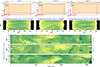 |
Fig. 1. Overview of the x − t maps generated from the synthetic 171 Å image sequence. Panel a1 illustrates the schematic of the simulation domain, where the orange hatched area outlines the volume we used to generate the synthetic image of case 1, shown in panel a2. The rectangular white box in panel a2 indicates the location and extent of the artificial slit we used to create the space-time (x − t) map displayed in panel a3. The two vertical lines in this x − t map define the time window during which decayless oscillations are observed. Cases 2 and 3 are presented in panels b1 to b3 and c1 to c3, respectively. |
4. Results
4.1. Decayless signatures
To analyze the decayless wave patterns, we zoomed into the regions in the space-time maps that covered only a few instances of decayless waves in neighboring threads. Examples are shown in Fig. 2, where we present zooms into the three x − t maps from Fig. 1. To enhance the visibility of the oscillating structures, we applied the multiscale Gaussian normalization (MGN) filter (Morgan & Druckmüller 2014) to produce these x − t maps. We identified several threads with persistent oscillations in all three maps. We emphasize that these decayless oscillations appear to be self-consistently from the model, and no prescribed driver was enforced.
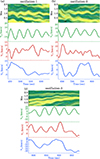 |
Fig. 2. Signatures of decayless oscillations in emission x − t maps and in the velocity components. Panel a presents signatures of oscillation-1 (from case-1). The top row in this panel displays a zoomed-in x − t map from Fig. 1, and the next three rows illustrate the time evolution of the velocity components vx, vy, and vz, respectively. The horizontal white lines indicate the δx extent of the 3D volume from which the velocity components were obtained (see Sect. 4.1 for more details). The other two panels (b and c) present information for oscillations 2 and 3 in the same format. |
Our analysis of these oscillating threads (see Appendix B) indicates that their periods range from 40 to 60 seconds, with typical amplitudes of about 0.1 Mm. The periods we observed in this study are consistent with those reported in earlier work. For example, applying the relation between the period and the loop length for standing modes of decayless oscillation in a loop measuring 50 Mm, we expect the period in our synthetic observations to be approximately 55 seconds (Shrivastav et al. 2024). This agrees well with the values we measured. Furthermore, the wave amplitude of 0.1 Mm is also typical for loop observations (e.g. Anfinogentov et al. 2015). Last, by examining the oscillation patterns derived from slits positioned at different locations along the loop, we confirm that these waves are the fundamental mode of standing decayless oscillations (see Appendix C).
The driver of these decayless oscillations now remains to be determined. As mentioned in the introduction, it is challenging to track field lines in space and time in these simulations. We therefore sought an indirect but effective proxy to understand the characteristics of the driver better. One such proxy is the wave polarization, and to understand this, we require the time evolution of the 3D velocity components associated with the oscillating plasma in the loop. From the previous analysis (mentioned in Section 3), we obtained δy values, and the location of the slits provided δz values. To determine the δx values, we manually identified the spatial extent of the oscillations in the x − t maps by plotting horizontal lines across each x − t map that fully covered the oscillating loop during the selected period while ensuring minimum overlap with other structures (see Fig. 2)1. Through this exercise, we identified the 3D volume that contained the section of the loop that is mapped onto the x − t map. The velocities we quote in the following sections are all averaged quantities within this identified volume.
In all three cases, clear oscillatory signals in vx are observed that do substantially decay over time for multiple cycles. While some degree of decay or modulation is present, it is far from the exponential decay that is typically observed in decaying oscillations. These oscillations in vx agree well with our findings in the synthesized emission maps. Furthermore, the periodicities in the FFT power spectrum of vx clearly peak at about 40 seconds. This value is quite similar to the periodicity of 43 seconds we obtained from the x − t map (see Appendix B).
The oscillations we show in Fig. 2 are most pronounced in the x direction and therefore in vx, as expected, because we conducted this analysis for instances of decayless waves that appear prominently in planes in which the line of sight is perpendicular to the x direction. The oscillatory nature of the vy and vz curves evident in all cases is a surprise, however. Combined with the oscillation in vx, it might indicate two possibilities: (1) The observed kink oscillations are not linearly polarized, that is, they might be elliptically or circularly polarized. (2) They are inherently linearly polarized, but the loop oscillation plane is tilted with respect to the line of sight, which results in oscillatory signals in the other velocity components. To investigate which of the two possibilities applies, we studied the hodograms for these waves.
4.2. Hodograms
One effective way to visualize the relations between different velocity components is through hodograms, which are parametric plots that illustrate the trajectory of a point with respect to two or more variables. To facilitate this, we first detrended the vx, vy, and vz curves so that the center of the hodograms showed no artificial shifts over time. The detrended curves are presented in Appendix B. In Fig. 3 we show the hodograms for each pair of vx, vy, and vz for all three oscillations displayed in Fig. 2.
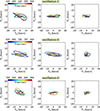 |
Fig. 3. Hodograms of the three decayless kink oscillations. In each instance, the colors in these hodograms represent the flow of time. Animated versions are available online. |
The vx versus vy hodograms in each oscillation show loopy elliptical structures that are mostly confined within a narrow band. The ellipse in oscillation-3 rotates slightly over time. The trajectories in the vx versus vz pairs are also elliptical, but they are much narrower because the vz values are significantly lower than the vx values. A similar pattern is observed in the vy versus vz hodograms.
Combining the information from all three hodograms for each oscillation, we find that all orbits in these plots are closed, which is characteristic of motion within a single plane. For intrinsically circularly polarized kink waves, elliptical (or circular) patterns are expected that share nearly identical properties, such as ellipticity or time evolution, in all three hodograms. The variation in ellipticity observed in the 2D projections agrees most consistently with linearly polarized kink waves that oscillate in planes that are tilted relative to all three axes. We therefore conclude that the decayless oscillations we observed are linearly polarized.
5. Discussion
We set out to explore the existence of decayless kink oscillations in loops in a 3D MHD simulation. We presented multiple examples of these oscillations that arose self-consistently, without an imposed driver in the simulation setup. All these decayless cases are fundamental-mode standing waves, whose antinode is located at the loop apex, and the nodes are positioned at the footpoint. We examine a few of our principal findings below.
A fundamental characteristic of these waves is their ubiquity. In nearly all instances, the wave persisted for approximately five cycles. This agrees well with the results of most observational investigations (Anfinogentov et al. 2013, 2015; Mandal et al. 2022; Shrivastav et al. 2024), although a few reports described decayless oscillations exceeding 30 cycles (e.g., Zhong et al. 2022). Nonetheless, whenever these oscillations were detected for fewer than five cycles, the physical state of the oscillating plasma (including its temperature or density) was proposed to have altered, which would have made the oscillating loop undetectable by the specific instrument filter or line employed for observation. In principle, the loop might therefore still oscillate, but this cannot be perceived. This hypothesis does not apply to our cases, however, because the velocity rapidly diminished after exhibiting four or five cycles of decayless signatures. This indicates that the field lines themselves did no longer oscillate. An explanation might be that during these oscillations, the loop gradually deviated from the particular 3D volume from which we extracted the velocity component (there was a slight trend in vy in all three instances), and the abrupt disappearance might therefore well be a manifestation of this behavior.
Another important diagnostic of decayless kink oscillations is the velocity amplitude, which constrains the wave energy content and is relevant for assessing their potential contribution to coronal heating when combined with an estimate of the effective dissipation rate. In our simulation, the vx values (representing the plane-of-sky motions) typically were approximately 10 km/s, while the line-of-sight component vy varied between 5 to 10 km s−1. These values are broadly consistent with those typically inferred from imaging and spectroscopic observations of decayless kink oscillations (e.g., Tian et al. 2012; Anfinogentov et al. 2013). Our simulation framework successfully reproduces transverse motions on the same order as found observationally overall.
We finally discuss the driver of the observed oscillations in the simulation. One challenge in identifying the driver is that it can operate at any point along the length of a magnetic field line, from the photosphere to the corona (i.e., from one footpoint to the next) and still produce decayless oscillations (Nakariakov et al. 2021). This makes the task quite complex, even in a simulation. The animation (associated with Fig. 3) shows that the loops in this simulation are highly dynamic. They drift and oscillate, likely reconnecting and altering their connectivity in the process. Consequently, it is challenging to identify the driver by tracking field lines throughout their entirety and throughout time. On the other hand, an indirect method of inferring the driver characteristics without the need to track a loop along its entire length is offered by studying the wave polarization properties. All individual cases we studied indicate that these decayless kink waves are largely polarized linearly and that their oscillation planes are tilted relative to the principal axes. These linearly polarized waves suggest that the driver preferentially excites waves in a specific direction. A source for this might be the self-oscillation model proposed by (Nakariakov et al. 2016). In this model, atmospheric flows (e.g., along supergranular boundaries) with a much longer characteristic timescale than the oscillation period drive these waves. This conclusion was also reached by Zhong et al. (2023). Although the oscillation planes appear to be rotating marginally with each oscillation cycle in oscillations 2 and 3, the patterns are still organized and stable. This indicates that a truly random or broadband footpoint motion is not a primary driver in these loops because these motions would yield disordered hodograms that vary in time and have an inconsistent shape and direction. It is important to note that our simulation setup lacks large-scale supergranular flows by design because the lower boundaries only span 6 × 6 Mm. This means that flows at other spatial scales must contribute to the decayless oscillation in our simulation. Finally, the lack of circularly polarized waves indicates that twisting or swirling motions probably do not cause these oscillations. This is particularly intriguing because the comparable 3D simulation presented by Breu et al. (2023) revealed swirls in the lower atmosphere that pumped a substantial amount of Poynting flux into the corona. It therefore remains unclear why these swirling motions fail to affect the decayless oscillation significantly. On the other hand, the elliptical shapes we observed might indeed signify this. Further investigations are necessary to examine this.
Another notable aspect is the tilt of the oscillation planes in each case, which might indicate a twist or writhe in the magnetic field. This twist might cause the loop to oscillate preferentially along a direction that is not perpendicular to the loop plane (Terradas & Goossens 2012). Furthermore, a varying twist in the field might also produce a variation in polarization (Terradas & Goossens 2012). This phenomenon is visible in some of the hodograms in Fig. 3. In this context, we note that Breu et al. (2022) reported a twist in several loop structures within this simulation setup (see Fig. 2 of their paper), which might indeed support our previous argument. The slight but consistent tilt of the vx − vy hodograms for each oscillation might also affect the straightened loop geometry chosen for this simulation, as well as the loop density contrast (Terradas et al. 2006). Finally, we note that the primary diagnostics for decayless kinks discussed above, namely period, phase, and polarization, are affected by loop-scale dynamics and are well resolved at our grid spacing of 60 km (consisting of hundreds of cells along a loop of approximately 50 Mm). In the MURaM simulations, numerical diffusion affects structures smaller than about five grid cells, however (approximately 300 km; Breu et al. 2025). While we consider our results to be robust regarding the overall kink behavior, we therefore do not claim convergence for small-scale dissipation or heating.
6. Prospects
Although the polarization states of the oscillation can reveal whether the wave driver is random or steady, they are unable to independently reveal some of the most important details about the driver. For example, the spatial placement of the driver, that is, whether it acts along the length of a loop or close to its footpoints, is not uniquely determined by the polarization states. We also require further investigations into the following facets of our findings: (i) whether the abrupt lack of oscillations arises from the loop exiting the selected analysis box; (ii) the extent to which twisting within the loops leads to similar oscillation polarization; and (iii) how the wave properties respond to changes in the photospheric magnetic environment of the numerical model, for example a transition from plage-like to sunspot-like conditions.
These investigations require tracking the field lines associated with the oscillating loops. Our current analysis is based on the visibility of loops in synthetic images, analogous to observations, which has certain limitations. For example, because of various changes in the plasma parameters, a loop may move in or out of the visibility range of a specific filter bandpass. Our current method therefore only allows us to capture a part of the loop evolution and not the whole process. Our current approach extracts information from a volume that is fixed in time. In reality, however, a loop may move laterally over time, meaning that it may not always be part of that volume (even though we selected the volume carefully). The dynamic appearance of these loops in the model also means that reliable field-line tracking becomes challenging nearer to the loop footpoints. This is particularly important for several wave properties. For instance, the presence of harmonics can only be meaningfully established by comparing oscillations at the loop apex with those in legs of the loop (Duckenfield et al. 2018). In short, the field lines that cover each oscillating structure must be followed in space at every time step. This is nontrivial because the field lines often reconnect along their lengths, which makes them harder to follow over time (Kohutova & Popovas 2021). A study that uses the existing field-line-tracing code used by Chen et al. (2022), is currently underway.
7. Conclusion
We provided evidence that decayless kink waves exist in long coronal loops. These waves emerge naturally from a 3D magnetohydrodynamic simulation. We further established the linear polarization states of these oscillations and emphasized that they favor a self-sustained or quasi-steady wave driver over a stochastic or broadband source.
Data availability
Movies associated to Figs. 3 and A.1 are available at https://www.aanda.org
Acknowledgments
We thank the anonymous reviewer for the encouraging comments and helpful suggestions. The work of S.M. was funded by the Federal Ministry for Economic Affairs and Climate Action (BMWK) through the German Space Agency at DLR based on a decision of the German Bundestag (Funding code: 50OU2201).
References
- Afanasyev, A. N., Van Doorsselaere, T., & Nakariakov, V. M. 2020, A&A, 633, L8 [NASA ADS] [CrossRef] [EDP Sciences] [Google Scholar]
- Anfinogentov, S., Nisticò, G., & Nakariakov, V. M. 2013, A&A, 560, A107 [NASA ADS] [CrossRef] [EDP Sciences] [Google Scholar]
- Anfinogentov, S. A., Nakariakov, V. M., & Nisticò, G. 2015, A&A, 583, A136 [NASA ADS] [CrossRef] [EDP Sciences] [Google Scholar]
- Aschwanden, M. J., Fletcher, L., Schrijver, C. J., & Alexander, D. 1999, ApJ, 520, 880 [Google Scholar]
- Breu, C., Peter, H., Cameron, R., et al. 2022, A&A, 658, A45 [NASA ADS] [CrossRef] [EDP Sciences] [Google Scholar]
- Breu, C., Peter, H., Cameron, R., & Solanki, S. K. 2023, A&A, 675, A94 [NASA ADS] [CrossRef] [EDP Sciences] [Google Scholar]
- Breu, C. A., De Moortel, I., Peter, H., & Solanki, S. K. 2025, MNRAS, 537, 2835 [Google Scholar]
- Chen, Y., Peter, H., Przybylski, D., Tian, H., & Zhang, J. 2022, A&A, 661, A94 [NASA ADS] [CrossRef] [EDP Sciences] [Google Scholar]
- Duckenfield, T., Anfinogentov, S. A., Pascoe, D. J., & Nakariakov, V. M. 2018, ApJ, 854, L5 [Google Scholar]
- Gao, Y., Guo, M., Van Doorsselaere, T., Tian, H., & Skirvin, S. J. 2023, ApJ, 955, 73 [NASA ADS] [CrossRef] [Google Scholar]
- Karampelas, K., & Van Doorsselaere, T. 2020, ApJ, 897, L35 [Google Scholar]
- Karampelas, K., & Van Doorsselaere, T. 2021, ApJ, 908, L7 [NASA ADS] [CrossRef] [Google Scholar]
- Karampelas, K., & Van Doorsselaere, T. 2024, A&A, 681, L6 [NASA ADS] [CrossRef] [EDP Sciences] [Google Scholar]
- Karampelas, K., Van Doorsselaere, T., Pascoe, D. J., Guo, M., & Antolin, P. 2019, Front. Astron. Space Sci., 6, 38 [Google Scholar]
- Kohutova, P., & Popovas, A. 2021, A&A, 647, A81 [NASA ADS] [CrossRef] [EDP Sciences] [Google Scholar]
- Lemen, J. R., Title, A. M., Akin, D. J., et al. 2012, Sol. Phys., 275, 17 [Google Scholar]
- Mandal, S., Tian, H., & Peter, H. 2021, A&A, 652, L3 [NASA ADS] [CrossRef] [EDP Sciences] [Google Scholar]
- Mandal, S., Chitta, L. P., Antolin, P., et al. 2022, A&A, 666, L2 [NASA ADS] [CrossRef] [EDP Sciences] [Google Scholar]
- Morgan, H., & Druckmüller, M. 2014, Sol. Phys., 289, 2945 [Google Scholar]
- Nakariakov, V. M., Ofman, L., Deluca, E. E., Roberts, B., & Davila, J. M. 1999, Science, 285, 862 [Google Scholar]
- Nakariakov, V. M., Anfinogentov, S. A., Nisticò, G., & Lee, D. H. 2016, A&A, 591, L5 [NASA ADS] [CrossRef] [EDP Sciences] [Google Scholar]
- Nakariakov, V. M., Anfinogentov, S. A., Antolin, P., et al. 2021, Space Sci. Rev., 217, 73 [NASA ADS] [CrossRef] [Google Scholar]
- Rempel, M. 2017, ApJ, 834, 10 [Google Scholar]
- Rochus, P., Auchère, F., Berghmans, D., et al. 2020, A&A, 642, A8 [NASA ADS] [CrossRef] [EDP Sciences] [Google Scholar]
- Shi, M., Van Doorsselaere, T., Guo, M., et al. 2021, ApJ, 908, 233 [Google Scholar]
- Shrivastav, A. K., Pant, V., Berghmans, D., et al. 2024, A&A, 685, A36 [NASA ADS] [CrossRef] [EDP Sciences] [Google Scholar]
- Skirvin, S. J., Gao, Y., & Van Doorsselaere, T. 2023, ApJ, 949, 38 [NASA ADS] [CrossRef] [Google Scholar]
- Terradas, J., & Goossens, M. 2012, A&A, 548, A112 [NASA ADS] [CrossRef] [EDP Sciences] [Google Scholar]
- Terradas, J., Oliver, R., & Ballester, J. L. 2006, ApJ, 650, L91 [NASA ADS] [CrossRef] [Google Scholar]
- Tian, H., McIntosh, S. W., Wang, T., et al. 2012, ApJ, 759, 144 [Google Scholar]
- Van Doorsselaere, T., Debosscher, A., Andries, J., & Poedts, S. 2004, A&A, 424, 1065 [NASA ADS] [CrossRef] [EDP Sciences] [Google Scholar]
- Vögler, A., Shelyag, S., Schüssler, M., et al. 2005, A&A, 429, 335 [Google Scholar]
- Zhong, S., Nakariakov, V. M., Kolotkov, D. Y., & Anfinogentov, S. A. 2022, MNRAS, 513, 1834 [NASA ADS] [CrossRef] [Google Scholar]
- Zhong, S., Nakariakov, V. M., Kolotkov, D. Y., et al. 2023, Nat. Commun., 14, 5298 [NASA ADS] [CrossRef] [Google Scholar]
Our results are not sensitive to the exact values of δx, δy, and δz that were used to derive the average velocities vx, vy, and vz that we analyzed.
Appendix A: An intriguing example
Not all the transverse oscillations observed in the simulation are decayless. Among them, we present an intriguing case in Fig. A.1. In this figure, oscillations, marked as oscillation-4.1 and oscillation-4.2, are seen in two adjacent loops. However, their appearance in the x-t map reveals that oscillation-4.1 is decayless in nature, while oscillation-4.2 exhibits signs of decay. This distinction becomes increasingly evident when we analyze the velocity components; we find that the velocity component vx of oscillation-4.1 shows only a slight decrease over time, whereas vx of oscillation-4.2 displays a rapid decay, resembling typical decaying kink oscillations. Constructed hodograms appear similar, further suggesting that both these these oscillations are most likely linearly polarized. Therefore, we have identified a case in which transverse oscillations occur simultaneously in two adjacent loops yet exhibit drastically different decay properties. Given that these two loops are most likely positioned at neighboring sites at the photospheric level, it is reasonable to conclude that they likely experience comparable footpoint driving conditions. It is indeed puzzling that they display distinct signatures of entirely contrasting regimes of kink oscillation and that too, simultaneously.
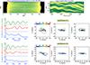 |
Fig. A.1. An example of co-existing decaying and decayless kink oscillations in neighboring loops. Top row shows the synthetic 171 Å image with the white rectangular box outlining the position of the artificial slit used to generate the x-t map shown in next panel. The slanted white and black dotted lines mark the δx values for the two selected oscillations. For more information on this, see Sect 4.1. The middle row displays the vx, vy and vz curves and the hodograms constructed for oscillation-4.1. The same but for oscillation-4.2 is shown in the bottom row panels. An animated version is available online. |
Appendix B: Detrended curves and periodicities
As mentioned in Section 4.2, the hodograms presented in Fig. 3 are constructed using the detrended velocity curves vx, vy, and vz. This same approach was also utilized for the hodograms shown in Fig. A.1. To determine the trend of a curve, we fit it with a best-fit polynomial (ranging from degree 1 to 5) and then subtract this fitted polynomial to obtain the final detrended curve. In Fig. B.1, we provide all the velocity curves for the oscillations discussed in this study.
The next step was to compute the periodicities present in these detrended velocity curves. We did this by performing a Fast Fourier Transform (FFT) on each curve. The results are presented in the bottom row of Fig. B.2 for two cases. The peak in vx (the plane-of-sky component) shows the strongest and most distinct feature in the FFT power spectrum, which is expected. Peaks in vy at the same period as vx are also observed, albeit much weaker. This pattern is similarly seen in vz. To compare the oscillations observed in the velocity components (especially vx) with those in the emission x-t maps, we fit the oscillating threads in the x-t maps using the following approach: first, we identify the location of an individual strand in the x-t map at each time step by fitting a Gaussian along the transverse direction of that strand. We then fit these derived positions of the strand as a function of time using the equation:
 (B.1)
(B.1)
where A is the oscillation amplitude, P represents the period, ϕ is the phase, and c0 and c1 are constants. Results based on these fits are shown in the top row of Fig. B.2.
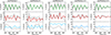 |
Fig. B.1. Original and detrended velocity curves for each oscillation. For a given oscillation, the original curves are shown in grey, while the detrended vx, vy, and vz curves are displayed with green, red, and blue lines, respectively. |
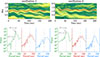 |
Fig. B.2. Estimation of oscillation periods based on the x-t maps and the velocity components. The top row of panels displays the x-t maps for oscillation-1 and oscillation-2. In these maps, dotted circles indicate the locations of the centers of the oscillating threads, while solid red curves represent the best-fit function (B.1) to those points. The estimated periods and amplitudes are shown on the panels. The bottom row of panels presents the FFT power spectrum for each velocity component: vx in green, vy in red, and vz in blue. The vertical dotted lines in these panels mark the locations of the dominant periods of vx, while the horizontal dashed lines outline the 95% significance level. |
Appendix C: Standing wave signatures
One of the critical aspect is to determine the mode of the observed decayless oscillation. To check this, we compare the phase difference between the oscillations captured via slits that are placed at a different position along the length of a loop. In Fig. C.1 we present two example, case-2 and case-4. In each case, we find no phase difference between oscillating threads, indicating that the observed oscillations are fundamental modes of standing waves.
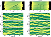 |
Fig. C.1. Identification of the wave mode through x-t maps. The left column shows the emission map (top panel) followed by x-t maps derived from the three slits indicated in the white rectangular boxes on the emission map. The dotted vertical lines mark the locations of the wave peaks and serve as a visual guide to identify the similarities or dissimilarities between oscillations. A similar analysis for case 4 is presented in the panels of the second column. |
All Figures
|
Fig. 1. Overview of the x − t maps generated from the synthetic 171 Å image sequence. Panel a1 illustrates the schematic of the simulation domain, where the orange hatched area outlines the volume we used to generate the synthetic image of case 1, shown in panel a2. The rectangular white box in panel a2 indicates the location and extent of the artificial slit we used to create the space-time (x − t) map displayed in panel a3. The two vertical lines in this x − t map define the time window during which decayless oscillations are observed. Cases 2 and 3 are presented in panels b1 to b3 and c1 to c3, respectively. |
| In the text | |
|
Fig. 2. Signatures of decayless oscillations in emission x − t maps and in the velocity components. Panel a presents signatures of oscillation-1 (from case-1). The top row in this panel displays a zoomed-in x − t map from Fig. 1, and the next three rows illustrate the time evolution of the velocity components vx, vy, and vz, respectively. The horizontal white lines indicate the δx extent of the 3D volume from which the velocity components were obtained (see Sect. 4.1 for more details). The other two panels (b and c) present information for oscillations 2 and 3 in the same format. |
| In the text | |
|
Fig. 3. Hodograms of the three decayless kink oscillations. In each instance, the colors in these hodograms represent the flow of time. Animated versions are available online. |
| In the text | |
|
Fig. A.1. An example of co-existing decaying and decayless kink oscillations in neighboring loops. Top row shows the synthetic 171 Å image with the white rectangular box outlining the position of the artificial slit used to generate the x-t map shown in next panel. The slanted white and black dotted lines mark the δx values for the two selected oscillations. For more information on this, see Sect 4.1. The middle row displays the vx, vy and vz curves and the hodograms constructed for oscillation-4.1. The same but for oscillation-4.2 is shown in the bottom row panels. An animated version is available online. |
| In the text | |
|
Fig. B.1. Original and detrended velocity curves for each oscillation. For a given oscillation, the original curves are shown in grey, while the detrended vx, vy, and vz curves are displayed with green, red, and blue lines, respectively. |
| In the text | |
|
Fig. B.2. Estimation of oscillation periods based on the x-t maps and the velocity components. The top row of panels displays the x-t maps for oscillation-1 and oscillation-2. In these maps, dotted circles indicate the locations of the centers of the oscillating threads, while solid red curves represent the best-fit function (B.1) to those points. The estimated periods and amplitudes are shown on the panels. The bottom row of panels presents the FFT power spectrum for each velocity component: vx in green, vy in red, and vz in blue. The vertical dotted lines in these panels mark the locations of the dominant periods of vx, while the horizontal dashed lines outline the 95% significance level. |
| In the text | |
|
Fig. C.1. Identification of the wave mode through x-t maps. The left column shows the emission map (top panel) followed by x-t maps derived from the three slits indicated in the white rectangular boxes on the emission map. The dotted vertical lines mark the locations of the wave peaks and serve as a visual guide to identify the similarities or dissimilarities between oscillations. A similar analysis for case 4 is presented in the panels of the second column. |
| In the text | |
Current usage metrics show cumulative count of Article Views (full-text article views including HTML views, PDF and ePub downloads, according to the available data) and Abstracts Views on Vision4Press platform.
Data correspond to usage on the plateform after 2015. The current usage metrics is available 48-96 hours after online publication and is updated daily on week days.
Initial download of the metrics may take a while.