From planetesimals to planets with N-body simulations in the giant-planet formation region

Sebastian Lorek; Michiel Lambrechts

doi:10.1051/0004-6361/202558429

Open Access

Issue		A&A Volume 707, March 2026


Article Number		A244
Number of page(s)		14
Section		Planets, planetary systems, and small bodies
DOI		https://doi.org/10.1051/0004-6361/202558429
Published online		17 March 2026

A&A, 707, A244 (2026)

From planetesimals to planets with N-body simulations in the giant-planet formation region

Sebastian Lorek^★ and Michiel Lambrechts

Center for Star and Planet Formation, Globe Institute, University of Copenhagen, Øster Voldgade 5-7, 1350 Copenhagen, Denmark

^★ Corresponding author: This email address is being protected from spambots. You need JavaScript enabled to view it.

Received: 5 December 2025
Accepted: 30 January 2026

Abstract

The cores of wide-orbit giant planets can form via pebble accretion if large planetesimals form in the outer regions of protoplanetary discs at sufficiently early times. Streaming instability simulations support mass distributions consistent with Solar System minor body constraints, but when and where planetesimal formation took place remains uncertain. Here, we report on our N-body simulations of core formation through pebble and planetesimal accretion starting from streaming-instability inspired planetesimal mass distributions. We explore two initial radial planetesimal distributions, a ring-like and a spatially more uniform distribution, between 10 and 50 AU. To address the numerical challenge of simulating realistic planetesimal numbers, corresponding to one to ten Earth masses of planetesimals, we made use of GPU acceleration for the N-body interactions (with GENGA) and a newly developed pebble accretion module. We find that the top of the planetesimal mass distribution provides the seeds for core formation through pebble accretion, leading to the formation of multiple giant planets. This is consistent with previous studies not including N-body interactions. Planetesimal surface densities, crudely corresponding to an initial 10% formation efficiency, imply low mean collision rates (around unity) in the gas disc phase. Our simulations show that giant planet formation depends only weakly on the initial locations where planetesimals form, because of rapid dynamical scattering, and on their total mass budget, due to filtering of the pebble flux between embryos. After disc dissipation, giant planet systems stir the remnant primordial planetesimals, making a scattered disc an inherent outcome of giant planet formation. Giant impacts between planetary cores generally appear to be rare in the first 100Myr.

Key words: methods: numerical / planets and satellites: formation

© The Authors 2026

Open Access article, published by EDP Sciences, under the terms of the Creative Commons Attribution License (https://creativecommons.org/licenses/by/4.0), which permits unrestricted use, distribution, and reproduction in any medium, provided the original work is properly cited.

This article is published in open access under the Subscribe to Open model. This email address is being protected from spambots. You need JavaScript enabled to view it. to support open access publication.

1 Introduction

In the core accretion scenario, giant planets form in the proto-planetary disc by first consolidating a solid core with a mass of around ten Earth masses, after which a H/He envelope is accreted (Mizuno 1980; Pollack et al. 1996). Such young gaseous proto-planetary discs contain a large mass reservoir of millimetre- to centimetre-sized icy dust particles called pebbles. Observations hint that discs around solar-mass stars frequently start out with pebble mass budgets in the range of tens to hundreds of Earth masses (Appelgren et al. 2023, 2025).

These pebbles are the likely building blocks of the first planetesimals, bodies larger than ten to one hundred kilometres in size. In the disc midplane, a dense pebble layer can become unstable to the streaming instability (Youdin & Goodman 2005). Subsequently, filaments form that then collapse by self-gravity into planetesimals (Johansen et al. 2007), with a mass distribution consistent with that of the minor body populations of the Solar System (Johansen et al. 2015; Simon et al. 2016; Schäfer et al. 2017).

Currently, it is unclear how efficient pebbles are converted into planetesimals. Historically, models for giant-planet core growth assumed high surface densities of planetesimals. However, such formation models only considering planetesimals still face challenges to forming giant planets within gas disc lifetimes (Pollack et al. 1996; Thommes et al. 2003; Coleman & Nelson 2014). For example, accretion cross-sections are low for primordial planetesimals larger than ten kilometres in size (Rafikov 2004), embryos deplete planetesimal feeding zones (Levison et al. 2010), and the migration of planetary cores may lead to planetesimal shepherding instead of accretion (Tanaka & Ida 1999; Johansen & Bitsch 2019).

In contrast, if planetesimal formation is less efficient, the remaining pebble mass fraction can be swept up by planetesimals, thus accelerating core growth. Small particles are efficiently accreted: Pebbles passing the planet spiral to the core due to gas drag and allow the planet to sweep up approximately 10% of the inwards drifting pebble flux (Ormel & Klahr 2010; Lambrechts & Johansen 2012). In the outer regions of the disc, where stellar irradiation dominates heating, this leads to insideout growth of embryos (Lambrechts & Johansen 2012; Ida et al. 2016). This allows cores to grow to completion under nominal pebble flux and pebble size ranges for solar metallicities and above (Lambrechts & Johansen 2014; Bitsch et al. 2015; Savvidou & Bitsch 2023; Gurrutxaga et al. 2024).

The N-body simulations that include pebble accretion show that a form of oligarchic growth, where only a handful of cores emerge, can be supported when large embryos stir neighbouring planetesimals out of the pebble midplane (Levison et al. 2015). However, these simulations ignore type-I migration. Subsequent N-body studies of giant-planet formation, including planetary migration, revealed a wide variety of planetary system architectures at disc dissipation, which later settle to stable multi-planet systems after the dissipation of the gas disc. (Matsumura et al. 2017; Bitsch et al. 2019; Wimarsson et al. 2020). Such N-body studies are valuable to initiate now in order to begin a comparison with the growing population of giant planets in wide orbits (Bitsch et al. 2020; Matsumura et al. 2021).

Such cold giants are now routinely detected through long-term radial velocity surveys and direct imaging. The occurrence rate of giant planets (≳0.1 Jupiter mass), located between 0.3 and 30 AU, is around 30% (Fulton et al. 2021). At wider orbits, direct imaging places a limit on the occurrence rate of around 5% of super-Jupiters (Nielsen et al. 2019; Vigan et al. 2021). The multiplicity of giant exoplanets is not well known. Kepler data support warm giants typically being in multiple systems (Mulders et al. 2018), and this is supported by radial velocity surveys as well (Mayor et al. 2011). At wider orbits, moderate eccentricities (e = 0.2-0.6) are common, hinting that these planets are also frequently located in multiples, although this may partly be a detection bias (Rosenthal et al. 2021, 2024).

In this work, we aim to investigate the growth from planetesimals to planets throughout the giant-planet formation region while taking pebble accretion into account. This is numerically challenging, and therefore previous works have frequently assumed the existence of planetary embryos to reduce the number of simulated particles. However, in order to understand the critical transition from the planetesimal formation and growth phase to the phase where embryos are sufficiently massive, it is important to have their growth dominated by pebble accretion (Liu et al. 2019), which sensitively depends on the assumed planetesimal mass distribution and surface density (Lorek & Johansen 2022). The objective of this work is not to perform exoplanet population synthesis (Matsumura et al. 2021) nor to explore the formation pathway of the Solar System (Raorane et al. 2024). Such explorations would require larger simulation suites to explore stochastic variations and different protoplane-tary disc conditions, such as the spread in their initial solid mass budgets, disc lifetimes, or heating mechanism.

It is not clear where the initial population of planetesimals formed, so we assumed a standard uniform distribution similar to Lau et al. (2024) but also one where planetesimals form in spatially separated rings. Because observed discs frequently show over- and under-dense pebble rings (Andrews 2020), it has been proposed that planetesimal formation may similarly be spatially non-uniform (Coleman & Nelson 2016). We, however, do not assume that these rings are associated with pressure bumps and do not explicitly model these in the gas disc (Morbidelli 2020; Brasser & Mojzsis 2020; Lau et al. 2022; Izidoro et al. 2022; Jiang & Ormel 2023).

Tracing the full planetesimal population will also allow us to understand directly what happens to the primordial population of planetesimals after planet formation has been completed. The formation of giant planets creates a scattered disc of minor bodies, which is a process that took place in the Solar System and is believed to be linked to the frequently observed debris discs around young stars (Wyatt 2020).

The paper is organised as follows. In Sect. 2 we provide an overview of the N-body method, the physical background model, the pebble accretion prescription, and the initial conditions for our simulations. In Sect. 3 we discuss the simulation results. In Sect. 4 we put our work into context. And finally, in Sect. 5, we summarise the main results.

2 Methods

In this section we outline the methods used in our N-body simulations of planet formation. In Sect. 2.1 we explain our choice for the protoplanetary disc. In Sect. 2.2 we detail the pebble accretion prescription, the choice of Stokes number, and the reduction of the pebble flux through accreting planets. In Sect. 2.4 we provide the equations for the gas accretion prescription we use to model the stage past the pebble isolation mass. In Sect. 2.5 we introduce the streaming-instability initial-mass function that determines the initial size distribution of the planetesimals in our simulations. In Sect. 2.6 we present the N-body method we chose for the simulations. Finally, in Sect. 2.7 we outline the initial conditions for our study. A summary of the parameters and their values used in our simulations is provided in Table 1.

Table 1

Simulation parameters and values.

2.1 Disc model

Viscous disc models are widely used to describe the structure of protoplanetary discs. In the steady state, the surface density, Σ_g, is determined by the accretion rate as $Σ_{g} = \frac{{\dot{M}}_{⋆}}{3 π ν},$ $Mathematical equation: \Sigma_\mathrm{g}=\frac{\dot{M}_\star}{3\pi\nu},$ (1)

where ν = αH²Ω_K is the viscosity of the gas in the α-disc model (Shakura & Sunyaev 1973). The parameter α is a nondimensional measure for the accretion velocity of the disc gas and is typically ~ 10⁻². The scale height, H, of the gas is the ratio of the sound speed, c_s, and the Keplerian frequency, Ω_K: H = c_s∕Ω_k. In order to use the steady-state approximation and the derived scaling laws, it is implicitly assumed that the disc size is larger than the simulated region of interest. Outside of the characteristic radius, the disc would expand instead (Lynden-Bell & Pringle 1974).

Hartmann et al. (2016) provides a fit to stellar accretion rates with time as $\log_{10} (\frac{{\dot{M}}_{⋆}}{M_{⊙} {y r}^{- 1}}) = - 7.9 - 1.07 \log_{10} (\frac{t}{M y r}),$ $Mathematical equation: \log_{10}\left(\frac{\dot{M}_\star}{M_\odot\,\mathrm{yr}^{-1}}\right)=-7.9-1.07\log_{10}\left(\frac{t}{\mathrm{Myr}}\right), \label{eq:MdotHartmann}$ (2)

scaled to a solar mass star. This gives Ṁ_*≈4.6 × 10⁻⁸ M_⊙ yr⁻¹ at 0.3 Myr and ~3.0 × 10⁻⁹ M_⊙ yr⁻¹ at 3.8Myr, which is in agreement with the lifetime of the solar nebula (Wang et al. 2017).

The scaling laws for surface density and temperature of an accretion disc in steady state are taken from Ida et al. (2016) and are based on the works of Chambers (2009) and Oka et al. (2011). In the inner disc, the temperature is set by viscous accretion, while the outer part of the disc is heated by stellar irradiation. When the accretion rate is 4.6 × 10⁻⁸ M_⊙ yr⁻¹, the boundary between the viscously heated and the illuminated disc will be at ~2.5 AU. As the mass accretion rate decreases to ~3 × 10⁻⁹ M_⊙ yr⁻¹, the boundary shifts inwards to ~0.25 AU at 3.8 Myr (using Eq. (2) for Ṁ_*). Because we are interested in the giant-planet formation region ≳10 AU that is well outside the viscously heated regime, we only take the irradiation into account. The power-law prescription for surface density has the form $Σ_{g} = 2.7 \times 10^{3} g {c m}^{- 2} {(\frac{α}{10^{- 3}})}^{- 1} (\frac{{\dot{M}}_{⋆}}{10^{- 8} M_{⊙} {y r}^{- 1}}) {(\frac{r}{A U})}^{- 15 / 14} .$ $Mathematical equation: \Sigma_\mathrm{g}=2.7\times10^3\,\mathrm{g}\,\mathrm{cm}^{-2}\,\left(\frac{\alpha}{10^{-3}}\right)^{-1} \left(\frac{\dot{M}_\star}{10^{-8}\,M_\odot\,\mathrm{yr}^{-1}}\right) \left(\frac{r}{\mathrm{AU}}\right)^{-15/14}.$ (3)

Here, the parameter α is the non-dimensional measure for the accretion velocity of the disc gas. The mass accretion rate is given by Eq. (2). The irradiated disc temperature (Ida et al. 2016) takes the form $T = 150 K {(\frac{r}{A U})}^{- 3 / 7} .$ $Mathematical equation: T=150\,\mathrm{K}\,\left(\frac{r}{\mathrm{AU}}\right)^{-3/7}.$ (4)

The pressure support of the disc is expressed as $η = - \frac{1}{2} {(\frac{H}{r})}^{2} \frac{\partial \log P}{\partial \log r},$ $Mathematical equation: \eta=-\frac{1}{2}\left(\frac{H}{r}\right)^2\frac{\partial \log P}{\partial \log r}, \label{eq:gaseta}$ (5)

with P being the gas pressure and H/r the aspect ratio of the gas disc. The logarithmic pressure gradient simplifies to ∂ log P∕∂ log r≈-2.8 for the given exponents of the surface density and temperature profiles.

2.2 Pebble accretion

The pebble accretion prescription is based on the work of Lambrechts et al. (2019b). We distinguish between the 3D accretion regime for low-mass embryos and the 2D regime for higher mass embryos. The first step to calculate effective pebble accretion rates is to determine pebbles sizes throughout the disc, which can differ significantly across the full disc range considered in this work.

2.2.1 Pebble Stokes number

The maximum size of the pebbles is determined by how fast micron-sized grains grow, fragment, and drift radially. Following the works of Birnstiel et al. (2012), Lambrechts & Johansen (2014), and Drążkowska et al. (2021), we assume that initially all grains are (sub-)micron in size with Stokes number St₀ and grow exponentially according to ${S t}_{g r o w t h} = {S t}_{0} \exp (\frac{t}{t_{g r o w t h}}),$ $Mathematical equation: \mathrm{St}_\mathrm{growth}=\mathrm{St}_0\exp\left(\frac{t}{t_\mathrm{growth}}\right),$ (6)

with a growth timescale, t_growth, of $t_{g r o w t h} = \frac{Σ_{g, 0}}{Σ_{d, 0}} Ω_{K}^{- 1} {(\frac{α_{m i d}}{10^{- 4}})}^{- 1 / 3} {(\frac{r}{A U})}^{1 / 3} .$ $Mathematical equation: t_\mathrm{growth}=\frac{\Sigma_{\mathrm{g},0}}{\Sigma_{\mathrm{d},0}}\Omega_\mathrm{K}^{-1}\left(\frac{\alpha_\mathrm{mid}}{10^{-4}}\right)^{-1/3}\left(\frac{r}{\mathrm{AU}}\right)^{1/3}.$ (7)

As the dust grows, collision velocities increase, and the maximum Stokes number is reached when the turbulent collision speeds equal the fragmentation velocity of the pebbles: ${S t}_{f r a g} = 0.37 \frac{v_{f r a g}^{2}}{3 α_{m i d} c_{s}^{2}},$ $Mathematical equation: \mathrm{St}_\mathrm{frag}=0.37\frac{v_\mathrm{frag}^2}{3\alpha_\mathrm{mid}c_\mathrm{s}^2}, \label{eq:stfrag}$ (8)

where υ_frag is the fragmentation velocity, which we assumed to be 1 ms⁻¹. Laboratory experiments argue for ~1 ms⁻¹ for the fragmentation velocity of silicates (Blum & Wurm 2008). For icy pebbles, however, the value of the fragmentation threshold velocity is debated and values range from ~10 m s⁻¹ (Gundlach & Blum 2015) to as high as ~50ms⁻¹ (Wada et al. 2009). However, more recent studies have shown that the sticking properties of water ice may be comparable to that of silicates for cold disc conditions, as is the case in the giant-planet region (Gundlach et al. 2018; Musiolik & Wurm 2019; Kimura et al. 2020). We therefore use 1 m s⁻¹ in our study.

If pebble drift faster than they can grow, the limiting Stokes number is ${S t}_{d r i f t} = \frac{1}{30 η} \frac{Σ_{d}}{Σ_{g}} .$ $Mathematical equation: \mathrm{St}_\mathrm{drift}=\frac{1}{30\eta}\frac{\Sigma_\mathrm{d}}{\Sigma_\mathrm{g}}.$ (9)

The factor 1/30 comes from the fact that the growth timescale needs to be ~30 times faster than the drift timescale for pebble growth to outperform radial drift (Okuzumi et al. 2012). When taking all the limiting cases into account, the actual Stokes number of the pebbles is $S t = max ({S t}_{0}, min ({S t}_{g r o w t h}, {S t}_{f r a g}, {S t}_{d r i f t})),$ $Mathematical equation: \mathrm{St}=\max\left(\mathrm{St}_0,\min\left(\mathrm{St}_\mathrm{growth},\mathrm{St}_\mathrm{frag},\mathrm{St}_\mathrm{drift}\right)\right),$ (10)

where we include St₀ because pebbles cannot be smaller than a single grain.

2.2.2 Pebble accretion rates

In the 3D regime, we use the minimum of the 3D accretion rate from Lambrechts et al. (2019b, their Eq. (A.13)), ṁ_L19, and the accretion rate for the accretion radius in the weak-coupling Bondi regime, ṁ_wc, found from their Eq. (A.5): ${\dot{m}}_{L 19} = \frac{1}{2 \sqrt{2 π}} \frac{m}{M_{⊙}} {(\frac{H_{p e b}}{H})}^{- 1} {(\frac{H}{r})}^{- 1} \frac{1}{η} F_{p e b},$ $Mathematical equation: \dot{m}_\mathrm{L19}&=\frac{1}{2\sqrt{2\pi}}\frac{m}{M_\odot}\left(\frac{H_\mathrm{peb}}{H}\right)^{-1}\left(\frac{H}{r}\right)^{-1}\frac{1}{\eta}F_\mathrm{peb}, \label{eq:mdotl19} \\$ (11) ${\dot{m}}_{w c} = π Σ_{p} r_{a c c, w c}^{2} (v_{r e l} + \frac{3}{2} Ω_{K} r_{a c c, w c}) \frac{Σ_{p e b}}{\sqrt{2 π} H_{p e b}} .$ $Mathematical equation: \dot{m}_\mathrm{wc}&=\pi\Sigma_\mathrm{p}r_\mathrm{acc,wc}^2\left(v_\mathrm{rel}+\frac{3}{2}\Omega_\mathrm{K}r_\mathrm{acc,wc}\right)\frac{\Sigma_\mathrm{peb}}{\sqrt{2\pi}H_\mathrm{peb}}.$ (12)

Here, H_peb/H is the ratio of pebble scale-height and gas scaleheight, η is related to the pressure gradient in the disc (Eq. (5)), and F_peb is the pebble flux.

The transition mass above which accretion changes from 3D to 2D to distinguish between the two regimes is $m_{2 D} = \frac{{(\sqrt{\frac{8}{π}} H_{p e b})}^{2} (δ v_{p} + \frac{3}{2} Ω_{K} \sqrt{\frac{8}{π}} H_{p e b})}{G t_{f}},$ $Mathematical equation: m_\mathrm{2D}=\frac{\left(\sqrt{\tfrac{8}{\pi}}H_\mathrm{peb}\right)^2\left(\delta v_\mathrm{p}+\frac{3}{2}\Omega_\mathrm{K}\sqrt{\tfrac{8}{\pi}}H_\mathrm{peb}\right)}{G t_\mathrm{f}},$ (13)

where t_f = StΩ_κ⁻¹ is the friction time of the pebbles, the accretion radius is $r_{a c c} = \sqrt{8 / π} H_{p e b}$ $Mathematical equation: $r_\mathrm{acc}=\sqrt{8/\pi}H_\mathrm{peb}$$ with pebble scale-height H_peb, and the accretion velocity is the velocity of the planet relative to the local circular orbit, δv_p, plus the shear at the accretion radius. For a circular, planar orbit δv_p = 0.

In the 2D regime, we used the maximum of the headwind-dominated, ṁ_hw, and shear-dominated, ṁ_sh, accretion rates given as ${\dot{m}}_{h w} = 2 Σ_{p e b} \sqrt{2 G m t_{f} v_{r e l}},$ $Mathematical equation: \dot{m}_\mathrm{hw}&=2\Sigma_\mathrm{peb}\sqrt{2Gmt_\mathrm{f}v_\mathrm{rel}}, \\$ (14) ${\dot{m}}_{s h} = 2 Σ_{p e b} \frac{3}{2} Ω_{K} {(\frac{4 G m t_{f}}{3 Ω_{K}})}^{2 / 3},$ $Mathematical equation: \dot{m}_\mathrm{sh}&=2\Sigma_\mathrm{peb}\frac{3}{2}\Omega_\mathrm{K}\left(\frac{4Gmt_\mathrm{f}}{3\Omega_\mathrm{K}}\right)^{2/3}, \label{eq:mdotshear}$ (15)

where v_rel is the relative velocity between the planet and the gas and m is the mass of the planet. Summarising Eqs. (11)-(15) for the 3D and 2D regimes, the actual pebble accretion rate is $\dot{m} = {\begin{cases} min ({\dot{m}}_{L 19}, {\dot{m}}_{w c}) & (m \leq m_{2 D}) \\ max ({\dot{m}}_{h w}, {\dot{m}}_{s h}) & (m > m_{2 D}) \end{cases} .$ $Mathematical equation: \dot{m}= \begin{cases} \min\left(\dot{m}_\mathrm{L19},\dot{m}_\mathrm{wc}\right) & \left(m\le m_{2\mathrm{D}}\right) \\ \max\left(\dot{m}_\mathrm{hw},\dot{m}_\mathrm{sh}\right) & \left(m> m_{2\mathrm{D}}\right) \end{cases} .$ (16)

2.2.3 Pebble isolation mass

Pebble accretion stops when the planet reaches the pebble isolation mass, M_iso (Lambrechts et al. 2014). Bitsch et al. (2018) finds $m_{i s o} = 25 M_{\oplus} {(\frac{H / r}{0.05})}^{3} \times (0.34 {(\frac{- 3}{\log_{10} α_{m i d}})}^{4} + 0.66) (1 - \frac{\frac{\partial \ln P}{\partial \ln r} + 2.5}{6}) .$ $Mathematical equation: m_\mathrm{iso}&=25M_\oplus\left(\frac{H/r}{0.05}\right)^3 \nonumber \\ &\times\left(0.34\left(\frac{-3}{\log_{10}\alpha_\mathrm{mid}}\right)^4+0.66\right)\left(1-\frac{\tfrac{\partial\ln{P}}{\partial\ln{r}}+2.5}{6}\right) \label{eq:pebisomass}.$ (17)

Here, P is the gas pressure and α_mid is the turbulent stirring strength of pebbles in the mid-plane.

2.2.4 Reduction of pebble flux

We include the reduction of the pebble flux through accreting planets as follows. The outermost planet receives the full pebble flux F₁ = F_peb of which it accretes per unit of time a fraction x₁ such that m₁ = x₁F₁. This reduces the pebble flux for the second outermost planet to F₂ = F₁-ṁ₁ = F₁(1-x₁). This planet would then accrete ṁ₂ = x₂F₂ = x₂(1-x₁)F₁. Extending this procedure, the pebble flux planet i receives is $F_{i} = F_{p e b} \prod_{k = 1}^{i - 1} (1 - x_{k}) .$ $Mathematical equation: F_i=F_\mathrm{peb}\prod_{k=1}^{i-1}(1-x_k). \label{eq:reducedpebflux}$ (18)

A planet that reaches pebble isolation mass cuts off the pebble flux to the planets located inside of its orbit. This approximation simplifies the interpretation of the results. However, coagula-tion/fragmentation studies show that small dust fragments may cross the planetary gap (Stammler et al. 2023).

2.2.5 Pebble flux

In our model, the pebble flux is set to a fixed fraction of the stellar mass accretion rate, $F_{p e b} = ξ {\dot{M}}_{⋆},$ $Mathematical equation: F_\mathrm{peb}=\xi\dot{M}_\star,$ (19)

with Ṁ_* given by Eq. (2) and ξ = 1.5%. Using viscous disc theory, it can be shown that the flux ratio ξ is related to the ratio of pebble and gas surface density: $\frac{Σ_{p e b}}{Σ_{g}} = \frac{ξ}{(2 / 3) | \partial \ln P / \partial \ln r | (S t / α) + 1}$ $Mathematical equation: \frac{\Sigma_\mathrm{peb}}{\Sigma_\mathrm{g}}=\frac{\xi}{\left(2/3\right)|\partial\ln P/\partial\ln r|\left(\mathrm{St}/\alpha\right)+1}$ (20)

(Johansen et al. 2019). Here, α is the accretion disc α value and not the midplane turbulence. In the case where St≲α, the flux ratio represents the metallicity Σ_peb/Σ_g of the disc, which is in our case 1.5%, slightly higher than the standard value of 1%. For St≳α, the local metallicity drops below the original value. Alternatively, the pebble flux could be set by fixing a pebble production rate at the outer edge of the disc (Lambrechts & Johansen 2014; Ida et al. 2016). In Fig. 1 we show the temporal evolution of the pebble flux and the total pebble mass drifting through the system. The pebble flux decreases from initially ~230 M_⊕ Myr⁻¹ to ~14 M_⊕ Myr⁻¹ at the end of the simulation. By integrating Eq. (19), the total mass of pebbles drifting through the system is ~163 M_⊕.

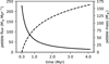Fig. 1

Pebble flux (solid) and total pebble mass (dashed) drifting through the system over time.

2.3 Migration

Migration, eccentricity, and inclination damping are implemented by applying additional accelerations, $a_{m} = - \frac{v}{t_{m}},$ $Mathematical equation: \mathbf{a}_\mathrm{m}&=-\frac{\mathbf{v}}{t_\mathrm{m}}, \\$ (21) $a_{e} = - 2 \frac{(v \cdot r) r}{r^{2} t_{e}},$ $Mathematical equation: \mathbf{a}_e&=-2\frac{\left(\mathbf{v}\cdot\mathbf{r}\right)\mathbf{r}}{r^2t_e}, \\$ (22) $a_{i} = - \frac{v_{z}}{t_{i}} k,$ $Mathematical equation: \mathbf{a}_i&=-\frac{v_z}{t_i}\mathbf{k},$ (23)

to each body. Here, t_m, t_e, and t_i are the respective timescales for migration and damping, and k is the unit vector in z direction (Cresswell & Nelson 2008).

Type I We used the timescales for migration, eccentricity, and inclination damping from Cresswell & Nelson (2008). The general damping timescale due to planet-disc interaction is $t_{w a v e} = \frac{M_{⋆}}{m} \frac{M_{⋆}}{Σ r^{2}} {(\frac{H}{r})}^{4} Ω_{K}^{- 1}$ $Mathematical equation: t_\mathrm{wave}=\frac{M_\star}{m}\frac{M_\star}{\Sigma r^2}\left(\frac{H}{r}\right)^4\Omega_\mathrm{K}^{-1}$ (24)

(Tanaka & Ward 2004). The damping timescale for eccentricity and inclination are $t_{e} = \frac{t_{w a v e}}{0.780} \times [1 - 0.14 {(\frac{e}{H / r})}^{2} + 0.06 {(\frac{e}{H / r})}^{3} + 0.18 (\frac{e}{H / r}) {(\frac{i}{H / r})}^{2}],$ $Mathematical equation: t_{e}&=&\frac{t_\mathrm{wave}}{0.780} \nonumber \\ &&\times\,\left[1-0.14\left(\frac{e}{H/r}\right)^2+0.06\left(\frac{e}{H/r}\right)^3+0.18\left(\frac{e}{H/r}\right)\left(\frac{i}{H/r}\right)^2\right], \label{eq:tdampe} \\$ (25) $t_{i} = \frac{t_{w a v e}}{0.544} \times [1 - 0.30 {(\frac{i}{H / r})}^{2} + 0.24 {(\frac{i}{H / r})}^{3} + 0.14 {(\frac{e}{H / r})}^{2} (\frac{i}{H / r})],$ $Mathematical equation: t_{i}&=&\frac{t_\mathrm{wave}}{0.544}\nonumber \\ &&\times\,\left[1-0.30\left(\frac{i}{H/r}\right)^2+0.24\left(\frac{i}{H/r}\right)^3+0.14\left(\frac{e}{H/r}\right)^2\left(\frac{i}{H/r}\right)\right], \label{eq:tdampi}$ (26)

and the migration timescale is $t_{m} = \frac{2 t_{w a v e}}{k_{m}} {(\frac{H}{r})}^{- 2} {P (e) + \frac{P (e)}{| P (e) |} \times [0.070 (\frac{i}{H / r}) + 0.085 {(\frac{i}{H / r})}^{4} - 0.080 (\frac{e}{H / r}) {(\frac{i}{H / r})}^{2}]},$ $Mathematical equation: t_\mathrm{m}&=&\frac{2t_\mathrm{wave}}{k_\mathrm{m}}\left(\frac{H}{r}\right)^{-2}\left\{P(e)+\frac{P(e)}{|P(e)|}\right.\\ &&\times\,\left.\left[0.070\left(\frac{i}{H/r}\right){+}0.085\left(\frac{i}{H/r}\right)^4{-}0.080\left(\frac{e}{H/r}\right)\left(\frac{i}{H/r}\right)^2\right]\right\}, \nonumber$ (27)

where $P (e) = \frac{1 + {(\frac{e}{2.25 H / r})}^{1.2} + {(\frac{e}{2.84 H / r})}^{6}}{1 - {(\frac{e}{2.02 H / r})}^{4}}$ $Mathematical equation: P(e)=\frac{1+\left(\frac{e}{2.25H/r}\right)^{1.2}+\left(\frac{e}{2.84H/r}\right)^6}{1-\left(\frac{e}{2.02H/r}\right)^4}$ (28)

(Cresswell & Nelson 2008) and k_m = 1.36+0.62q_S+0.43p_T (D’Angelo & Lubow 2010), with q_s = 15/14 and p_T = 3/7 being the power-law exponents of surface density and temperature, respectively.

Type II The transition to type-II migration occurs for (partially) gap-opening planets exceeding the pebble isolation mass. We implement this transition by multiplying the type-I migration timescale, t_m, with the correction factor $\frac{Σ_{g a p}}{Σ} = \frac{1}{1 + {(m / (2.3 m_{i s o}))}^{2}},$ $Mathematical equation: \frac{\Sigma_\mathrm{gap}}{\Sigma}=\frac{1}{1+\left(m/(2.3\,m_\mathrm{iso})\right)^2},$ (29)

which is the ratio of the gas surface density in the gap, Σ_gap, to the unperturbed surface density (Kanagawa et al. 2018; Ida et al. 2018; Johansen et al. 2019).

2.4 Gas accretion

The planets in our simulations were allowed to accrete gas once they reached pebble isolation mass. In the first phase, the atmosphere grows through Kelvin-Helmholtz contraction: ${\dot{m}}_{K H} = 10^{- 5} M_{\oplus} {y r}^{- 1} {(\frac{m}{100 M_{\oplus}})}^{4} {(\frac{κ}{0.1 {k g}^{- 1} m^{2}})}^{- 1}$ $Mathematical equation: \dot{m}_\mathrm{KH}=10^{-5}\,M_\oplus\,\mathrm{yr}^{-1}\left(\frac{m}{100\,M_\oplus}\right)^4\left(\frac{\kappa}{0.1\,\mathrm{kg}^{-1}\,\mathrm{m}^2}\right)^{-1}$ (30)

(Ikoma et al. 2000). Here, κ is the opacity of the atmosphere.

A second contribution to gas accretion is the accretion of the disc gas that enters the Hill sphere of the planet during runaway gas accretion. Lambrechts et al. (2019a) provide a fit to hydrodynamic simulations that quantifies the amount of the gas that is bound in the growing atmosphere: ${\dot{m}}_{H} = 2.7 \times 10^{- 3} M_{\oplus} {y r}^{- 1} {(\frac{m}{100 M_{\oplus}})}^{1.9} .$ $Mathematical equation: \dot{m}_{\mathrm{H}}=2.7\times10^{-3}\,M_\oplus\,\mathrm{yr}^{-1}\left(\frac{m}{100\,M_\oplus}\right)^{1.9}.$ (31)

Lastly, the maximum amount of gas that can be accreted is provided by the stellar gas accretion rate, Ṁ_*. We therefore used the minimum of the three accretion rates as the actual gas accretion rate of the planet: $\dot{m} = min ({\dot{m}}_{K H}, {\dot{m}}_{H}, {\dot{M}}_{⋆}) .$ $Mathematical equation: \dot{m}=\min(\dot{m}_\mathrm{KH},\dot{m}_{\mathrm{H}},\dot{M}_\star).$ (32)

2.5 Planetesimal sizes

Collisional growth of dust and ice grains forms millimetre- to centimetre-sized pebbles throughout the disc. These pebbles are concentrated in filaments by the streaming instability and subsequently collapse gravitationally into planetesimals (Youdin & Goodman 2005; Johansen et al. 2014; Li et al. 2018). The initial mass function (IMF) of planetesimals is an ongoing research question (Johansen et al. 2015; Schäfer et al. 2017; Li et al. 2019; Simon et al. 2022; Gerbig & Li 2023). While the steep upper end of the IMF is found to be similar to the observed size distribution of cold classical Kuiper belt objects (Kavelaars et al. 2021), the lower end depends on resolution (Li et al. 2019). Here we use an exponentially tapered power law (Schäfer et al. 2017). For masses below a characteristic planetesimal mass, the IMF follows a power law with exponent ~0.6. Above the characteristic mass, the IMF drops exponentially limiting the maximum mass to ~10⁻³−10⁻¹ M_⊕, depending on the distance from the star. A note on nomenclature, here we use the term embryo for the top of the IMF, bodies usually in the range 10⁻³−10⁻¹ M_⊕.

The IMF can be expressed as the cumulative number of bodies with a mass higher than m: $\frac{N (> m)}{N_{t o t}} = {(\frac{m}{m_{m i n}})}^{- p} \exp [{(\frac{m_{m i n}}{m_{p}})}^{q} - {(\frac{m}{m_{p}})}^{q}],$ $Mathematical equation: \frac{N(>m)}{N_\mathrm{tot}}=\left(\frac{m}{m_\mathrm{min}}\right)^{-p}\exp\left[\left(\frac{m_\mathrm{min}}{m_\mathrm{p}}\right)^q-\left(\frac{m}{m_\mathrm{p}}\right)^q\right], \label{eq:imf}$ (33)

where m_p is the characteristic planetesimal mass at which the exponential drop-off starts and m_min≪m_p is a minimum mass (Schäfer et al. 2017). We used an approximate scaling law for the characteristic planetesimal mass, m_p, that was derived in Liu et al. (2020) by compiling streaming instability simulations. The expression for m_p reads as $m_{p} = 5 \times 10^{- 5} M_{\oplus} (\frac{C}{5 \times 10^{- 5}}) {(\frac{Z}{0.02})}^{0.5} {(\frac{γ}{π^{- 1}})}^{1.5} {(\frac{H / r}{0.05})}^{3} (\frac{M_{⋆}}{M_{⊙}}),$ $Mathematical equation: m_\mathrm{p}=5\times10^{-5}\,M_\oplus\left(\frac{C}{5\times10^{-5}}\right)\left(\frac{Z}{0.02}\right)^{0.5}\left(\frac{\gamma}{\pi^{-1}}\right)^{1.5}\left(\frac{H/r}{0.05}\right)^3\left(\frac{M_\star}{M_\odot}\right),$ (34)

where C is a parameter to match the scaling law to streaming instability simulations, Z is the metallicity of a streaming instability filament, γ = 4πGρ_g/Ω_K² is a measure for the relative strength between self-gravity and shear and M_* is the stellar mass. To convert from mass to radius, we use a constant density of 2 g cm⁻³. We do not employ an explicit mass-radius relationship (e.g. Seager et al. 2007).

2.6 GPU-accelerated N-body simulations

We used the Gravitational Encounters with GPU Acceleration (GENGA) code (Grimm & Stadel 2014; Grimm et al. 2022) for N -body simulations of planet formation. We added the effects of pebble accretion, gas accretion, and migration to simulate the formation process in the nebular phase. Using GENGA, we were able to include several thousand bodies in the simulations to self-consistently follow the growth of a size distribution of bodies, drawn from streaming instability simulations as described in detail in Sect. 2.5, ranging from ~200 km-sized planetesimals to ~0.1 M_⊕ embryos.

We implemented our pebble and gas accretion prescriptions as CUDA kernels in GENGA. The new kernels are called each time step in the N-body step of GENGA. While the gas accretion kernel affects each planet individually, the reduction of the pebble flux in the pebble accretion kernel requires knowledge of the radial order of all the planets in the simulation. To achieve this, we firstly calculated the accretion efficiency x_i = ṁ_i/F_i of each pebble-accreting planet, which is independent of the pebble flux. In a next step, we sorted the planets according to their radial distance from the central star. With the sorted list of planets, we proceeded by calculating the reduced pebble flux for each planet (Eq. (18)). Finally, we calculated the accreted mass in pebbles by multiplying the accretion efficiency x_i with the reduced flux F_i.

2.7 Initial conditions

We placed the simulations in the giant-planet formation region between 10 and 50 AU and integrated the nebular phase for 3.8 Myr from 0.3 Myr until 4.1 Myr with a time step of 12 days. This assumed lifetime of the gas disc lies in the estimated range of lifetimes for the gas disc around the Sun of 2.51-4.89 Myr after CAI formation (i. e. after t = 0; Wang et al. 2017; Weiss et al. 2021). After 4.1 Myr, the runs were extended to 100 Myr in the gas-free phase.

We explored two initial spatial distributions for the planetesimals. One setup where the planetesimals were distributed in spatially separated narrow rings (narrow rings henceforth) and one where we started with a uniform distribution in a single wide ring (wide ring henceforth). For narrow rings, we placed all planetesimals in four rings each of width ηr that is the typical width of a streaming instability filament (Yang & Johansen 2014; Liu et al. 2019; Gerbig et al. 2020). For the wide rings, we placed the planetesimals such that the rings connected. Each ring had constant surface density determined by the filament metallicity Z_fil meaning that the initial surface density of the planetesimals followed the gas surface density with slope 15/14(≈1).

In each case, we numerically sampled the IMF, where we set the minimum mass m_min = 5 × 10⁻³ m_p, p = 0.6, and q = 0.35 (Schäfer et al. 2017). This led to planetesimal populations ranging from ~200km to about 0.1 M_⊕, depending on semi-major axis, with small planetesimals dominating in number, but larger embryos dominating in mass. Figure 2 shows the initial complementary cumulative mass distribution (CCDF) of planetesimals averaged over all runs in the wide and narrow ring simulations. The maximum embryo mass is of the order ~0.1 M_⊕ (~Mars mass) while 50% of the mass is in planetesimals less massive than ~2 × 10⁻³ M_⊕ (~Pluto mass). The maximum embryo mass varied from run to run because of the random sampling of the IMF.

To determine the total mass of the planetesimals, we first determined the total mass of a streaming instability filament: $M_{f i l} = 2 π r Σ_{g} Z_{f i l} η r .$ $Mathematical equation: M_\mathrm{fil}=2\pi r\Sigma_\mathrm{g}Z_\mathrm{fil}\eta r.$ (35)

Here we assumed that the dust-to-gas ratio of the filament, Z_fil, is given as the maximum of, firstly, the Stokes-number-dependent criterion of Yang et al. (2017), $\log Z_{c} = {\begin{cases} 0.30 {(\log S t)}^{2} + 0.59 \log S t - 1.57 & (S t > 0.1), \\ 0.10 {(\log S t)}^{2} + 0.20 \log S t - 1.76 & (S t < 0.1), \end{cases}$ $Mathematical equation: \log{Z_\mathrm{c}}= \begin{cases} 0.30\left(\log\mathrm{St}\right)^2+0.59\log\mathrm{St}-1.57 & \left(\mathrm{St}{>}0.1\right), \\ 0.10\left(\log\mathrm{St}\right)^2+0.20\log\mathrm{St}-1.76 & \left(\mathrm{St}{<}0.1\right), \end{cases}$ (36)

and, secondly, the dust-to-gas ratio that is obtained from balancing vertical settling and diffusion, $Z_{s e t t} = \sqrt{α_{m i d} / (α_{m i d} + S t)}$ $Mathematical equation: $Z_\mathrm{sett}=\sqrt{\alpha_\mathrm{mid}/\left(\alpha_\mathrm{mid}+\mathrm{St}\right)}$$ .

In this way, we obtained Z_fil = max (Z_c, Z_sett). The total mass in planetesimals was then M_tot = p_eff M_fil, with p_eff describing a planetesimal formation efficiency that is not very well constrained. Variations from ≲10 to 80% have been observed in simulations (Abod et al. 2019). With p_eff = 10%, representing the lower end of possible values, we end up with a total mass of planetesimals in the 10-50 AU region of ~1 M_⊕. With p_eff = 100%, we would obtain M_tot~10 M_⊕, which we used for the high-mass simulations.

Eccentricities and inclinations were sampled from Rayleigh distributions with respective root mean square values of 10⁻⁵and 5 × 10⁻⁶. We chose low initial values of eccentricity and inclination because the combination of mutual scattering and gas drag leads to rapid excitation and damping, rendering the initial choice unimportant. Arguments of perihelion, longitudes of ascending node, and mean anomalies were sampled from uniform distributions in the range from 0 to 2π.

For each initial configuration, narrow rings and wide rings, we ran a total of six simulations with randomised initial configurations of planetesimals. This provides a small statistical sample for further analysis. The simulations are labelled n05 to n10 for narrow ring runs and w03 to w08 for wide ring runs. We ran an additional set of six simulations with a total planetesimal mass of ~10 M_⊕, which are labelled m01 to m06. The low-mass simulations typically contained around 4000 fully interacting bodies. The high-mass simulations were divided into ~4000 fully interacting bodies and ~36 000 semi-active test particles that did not interact with each other but interacted gravitationally with the fully interacting bodies. The mass below which bodies are considered test particles was set to 10⁻³ M_⊕, which is approximately the transition mass below which pebble accretion becomes inefficient evaluated at ~3.6AU (Lambrechts & Johansen 2012; Ormel 2017).

The high number of bodies per simulation led to run times of several days for the low-mass rings and up to weeks for the highmass rings, which rendered it difficult to obtain larger sets due to limited computational resources. We used Nvidia A30 GPUs in Multi-Instance GPU (MIG) configuration of four instances for the low-mass runs. The run times ranged from 33 to 131 hours (1.4-5.5 days) with an average of 56.2 hours (2.3 days) per simulation. For the high-mass runs we used the full capacity of the Nvidia A30 GPU. The run times were 146 to 309 hours (6.1-12.9 days) with an average of 197 hours (8.2 days) per simulation. The total number of 115 662 000 time steps and the output interval of one output every 100 000 time steps were the same for each low- and high-mass run. Table 1 summarises the parameters used in each simulation and Table 2 lists the initial ring locations for the narrow and wide ring runs.

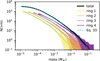Fig. 2

Initial planetesimal mass distribution. We show the initial distributions of the rings (solid coloured lines), the total distribution of all bodies (black), and Eq. (33) (dashed cyan lines). All distributions have been averaged over all low-mass runs. The standard deviation (shaded area) shows the spread of the initial planetesimal mass distribution from the random sampling. The high-mass runs follow the same IMF but with a higher total number of bodies (see also Fig. 8).

Table 2

Initial ring locations.

3 Results

To describe the planets formed in our simulations, we used mass categories to cover planetesimals (<10⁻³ M_⊕), Pluto- to Marsmass bodies (10⁻³−0.1 M_⊕ ), terrestrial-like planets (0.1-2 M_⊕), super-Earths (2-10 M_⊕), ice-giants (10-80 M_⊕), and gas giants (>80 M_⊕). This was motivated by the different types of planets found in the Solar System and exoplanetary systems. Because N-body simulations are stochastic, the outcome of individual simulations varies in terms of, for example, the number of planets formed or their final configuration. Before summarising and comparing the outcome of each set of simulations, we describe the typical evolution for the case of a single run.

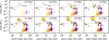Fig. 3

Snapshots of mass and semi-major axis from 0.3 to 4.1 Myr for narrow ring run n05. The initial locations of the rings are 12.2 AU (yellow), 18.3 (orange), 27.3 (red), and 40.9 AU (purple). The symbol size scales with the mass of the body as ∝ m^1/3. Planets with mass ≥0.1 M_⊕ have solid circles. The Solar System planets (+) and Pluto and Eris (◇) are shown for reference as well as the pebble isolation mass (dashed line).

Fig. 4

Same as Fig. 3 but showing the eccentricity and semi-major axis evolution.

3.1 Example narrow ring run n05

3.1.1 Nebular phase

In the nebular phase, gas is present until disc dissipation at 4.1 Myr. Figure 3 illustrates core growth due to pebble accretion and mutual collisions in narrow ring run n05. Figure 4 shows the eccentricity versus semi-major axis for all bodies in this simulation.

From initially narrow rings with low eccentricity, the top of the mass distribution grows by collisions and pebble accretion. These embryos, while embedded in the rings, start to dynamically excite the smaller planetesimals to higher eccentricities (and inclinations). While the lower-mass planetesimals gain higher eccentricities and inclinations, the higher-mass embryos acquire lower eccentricities and inclinations because of dynamical friction and eccentricity and inclination damping (Ida & Makino 1992; Cresswell & Nelson 2008). Furthermore, this excitation causes a significant broadening of the initially narrow rings (Ohtsuki & Tanaka 2003; Tanaka et al. 2003), especially towards later times (≳ 1.5 Myr).

We observe that bodies in the innermost ring located at ~12AU grow faster than the ones located farther out, even though they were seeded with initially higher masses. This is a consequence of the inside-out growth behaviour of pebble accretion in an irradiated protoplanetary disc, where the pebble accretion timescale decreases with increasing distance from the star (Lambrechts & Johansen 2014). As the two most massive bodies in the innermost ring grow, they start to migrate at ~ 1.5 Myr, which causes depletion of the ring and smaller planetesimals to be dragged along. At ~ 1.9 Myr, one of the two planets reaches pebble isolation mass marking the onset of gas accretion. This planet continues to grow and migrate until the transition to type-II migration and disc dissipation slow down and finally stop its inwards motion at ~5 AU. The lowermass companion also continues to migrate. Because this planet is inside the orbit of the other one, it does not continue to accrete pebbles because in our model a planet that reaches pebble isolation mass cuts off the pebble flux. Hence, this ~1-2 M_⊕ planet does not grow and continues fast type-I migration until disc dissipation stops migration at ~0.6AU. Towards the very end of the simulation at ~3.7 Myr, this planet crosses the pebble isolation mass line and accretes a tiny amount of gas.

In addition to the gas giants, several planets with masses in the terrestrial to the ice giant range form in the outer rings. These planets do not migrate far and remain closer to their birth location in the 10-50 AU region. The planet masses tend to decrease with distance, which is again a consequence of the inside-out growth. Towards the end of the nebular phase, the gas giant and the planets still embedded in their birth environment excite the remaining planetesimals and produces a scattered disc-like structure containing planetesimals from the two innermost rings, that is the population originally located between ~10 and 25 AU.

Fig. 5

Same as Fig. 3 but for 4.1-100 Myr.

Fig. 6

Same as Fig. 4 but for 4.1-100 Myr.

3.1.2 Gas-free phase

After disc dissipation at 4.1 Myr, we integrated run n05 in the gas-free phase until 100Myr. Figures 5 and 6 illustrate the evolution of mass and eccentricity versus semi-major axis for all bodies in this simulation.

When the gas disc dissipates, the damping effect of the gas on the orbits of the planets and planetesimals disappears. This leads to strong dynamical excitation of eccentricities and inclinations, depletion of planetesimals and planets by ejection, and mixing of the rings such that memory of the initial distribution is completely lost. A total mass of ~1.5 M_⊕ is ejected, whereof 0.2 M_⊕ are planetesimals with mass ≤10⁻³ M_⊕, 0.6 M_⊕ are Pluto- to Mars mass bodies (10⁻³−0.1 M_⊕), and 0.7 M_⊕ are terrestrial-like planets (0.1 −2 M_⊕). In numbers, ~ 1400 planetesimals, 88 Pluto-to Mars mass bodies, and 3 terrestrial-like planets are lost over the 100 Myr of evolution. Noteworthy is the formation of a scattered-disc-like structure consisting of planetesimals and embedded planets extending from ~20-30AU to up to ~200 AU in semi-major axis. Such a scattered disc is formed in all our simulations, regardless of the initial distribution of planetesimals.

3.2 Collisions

Most collisions occur in the first 0.1 Myr when the surface densities of planetesimals are high. As time goes on, collisions become less frequent. Figure 7 shows the projectile-to-target ratio as a function of time for the narrow and wide ring runs n05 and w05 from 0.3 to 100Myr. Initially, the mass ratio of projectile and target is ≳10⁻² and most collisions are between planetesimals or between the top of the mass distribution and planetesimals. At later times and after the disc dissipated, the mass ratio of projectile and target decreases with time and is typically ≲10⁻². This indicates that collisions are dominantly between a planet-sized body and a much smaller planetesimal. Giant impacts between planetary cores with a mass ratio ≳0.1 appear to be typically rare. However, we integrated for only 100 Myr, on longer Gyr timescales this may change and we leave this for future work.

Generally, giant impacts appear to be rare in the giant-planet formation region within the first 100 Myr of evolution. In the Solar System, giant impacts are linked to the Moon-forming impact (t≈50-100Myr; Canup 2004; Thiemens et al. 2019), and potentially to the obliquities of Uranus and Neptune (Morbidelli et al. 2012; Izidoro et al. 2015; Kegerreis et al. 2018; Reinhardt et al. 2020; Esteves et al. 2025, but see also e.g. Boué & Laskar 2010 and Saillenfest et al. 2022 for a non-impact mechanism). It is challenging to place our results in the context of giant impacts in the Solar System, as we do not model terrestrial planet formation, and giant impact probabilities, conditional on the presence of four giant planets, would require a much larger simulation suite than presented in this work.

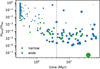Fig. 7

Collisions as a function of time. We show the projectile-to-target mass ratio for each collision for runs n05 (green) and w05 (blue) from 0.3 to 100 Myr. Each symbol shows a single collision. The nebular phase ends at 4.1 Myr (dashed line). The symbol size scales with the mass of the target as ∝m^1/3.

3.3 Mass distribution

Figure 8 shows the mean complementary cumulative mass distribution, that is the number of bodies larger than mass m, at the end of the nebular phase at 4.1 Myr and, for comparison, the initial distribution for each set of simulations (Table 2). For all three cases, the mass distributions are similar for planetesimals (<10⁻³ M_⊕) and resemble the initial distribution showing that neither collisions nor pebble accretion result in significant growth of this population. For planets more massive than ~1-2 M_⊕ , the distributions are comparable as well. This indicates that neither the initial distribution nor the total mass in planetesimals significantly impact the final number of planets.

However, in the low-mass runs, bodies in the mass range ~10⁻³−1 M_⊕ are depleted by up to a factor ~4 in the narrow ring runs compared to the wide rings. This is a consequence of the reduction of pebble accretion efficiency due to dynamical excitation of the pebble accreting bodies (Levison et al. 2015; Lau et al. 2024). Because of the higher spatial concentration of planetesimals in the narrow rings compared to the wide rings, encounter rates are higher and planetesimal scattering results in higher eccentricities and inclinations. Therefore, the relative velocities between pebbles and planetesimals are higher for the narrow rings, especially in earlier times before high-mass planets dominate the scattering and erase the effect of the initial conditions. Because our pebble accretion prescription accounts for the relative velocity between the accreting body and the pebbles, higher relative velocities lead to shorter encounter times, and consequently, the weak-coupling accretion rate applies, which lowers the efficiency for pebble accretion. For higher mass planets, eccentricity and inclination damping circularises their orbits and this effect vanishes. This explains why bodies in the mass range ~10⁻³−1 M_⊕ grow less efficiently in the narrow rings.

We ran a set of simulations with an initially higher total mass of planetesimals of ~10 M_⊕ (runs m01 to m06) to study whether this affects the final mass distribution of planets. Comparing the high-mass wide rings with the low-mass wide rings (Fig. 8), shows that the number of planets ≳ 1 M_⊕ are comparable, whereas the number of lower-mass bodies is higher. The higher number of lower-mass bodies is a natural consequence of the higher number of planetesimal seeds. The self-regulation of the number of ≳ 1 M_⊕ planets is due to mutual filtering, which we discuss in more detail in Sect. 3.5.

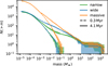Fig. 8

Mass distribution at 4.1 Myr. We show the average mass distributions for the narrow (green), wide (blue), and high-mass wide (orange) rings at 4.1 Myr (solid lines) with respective standard deviation (shaded area). The initial distributions (dashed lines) are shown for comparison.

3.4 Final configuration of planets

The final configuration of planets for all simulation runs is summarised in Fig. 9. We start with the configuration of the planets. In all our simulations we find that the most massive planets, that is those that evolve into gas giants, migrate inwards and end up in the range ~2-10 AU. Lower-mass planets, that is those in the terrestrial to super-Earth range, are predominantly found outside the orbit of the gas giants with semi-major axis ~6-50 AU. These planets form and remain closely to the initial location of the planetesimal disc. The same holds for ice giants, even though in two runs (w07 and m05), one ice giant respectively ends up in the range 1-2 AU, inside the orbit of the giant planet. During formation, these two ice giants got dragged along inwards by the giant planet and continued to migrate. The same occurred in run m06 for the terrestrial-like planet that ended up close to 1AU.

Figure 10 summarises how many planets in each mass category ≥1 M_⊕ form in our simulations. Ice and gas giants are typically rare. Regardless of the initial distribution and initial total mass of planetesimals, at most two gas giants are formed and at most one ice giant per run. The rare occurrence of ice giants may be a consequence of the pebble isolation mass falling in the same mass range in the 10-50 AU range. Therefore, if planets grow too slowly, they will end up with masses less than 10 M_⊕, and, on the other hand, if they grow more quickly and reach pebble isolation mass, they will continue to grow to gas giants by rapid gas accretion. In the mass range 2-10 M_⊕, roughly the same number of ~2-6 planets are formed in the low- and high-mass wide ring runs. The narrow rings show a higher variation because run n09 did not form any planets in this mass range. Excluding this specific run, however, shows that also the remaining narrow ring runs produce 2-5 planets in the super-Earth regime. Finally, going to planets ≲2 M_⊕, we find that the narrow rings form the lowest number of planets in this mass range. Typically, we find one to three planets, excluding runs n06 and n10 that did not form any planets in this mass range.

The wide ring runs form one to five planets, and the highmass wide ring runs form three to seven planets in this range. It is worth noting that, based on these numbers, the initial configuration and the initial total mass of the planetesimals have only minor influence on the planetary systems formed.

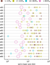Fig. 9

Configuration of planets at 4.1 Myr. Each row shows the configuration of planets ≥1 M_⊕ at 4.1 Myr. The runs we show are as follows: narrow ring runs (n05-n10, top), wide ring runs (w03-w08, middle), and high-mass ring runs (m01-m06, bottom). The symbol size scales with the mass of the body as ∝m^1/3, and the colour indicates the mass category.

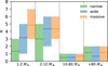Fig. 10

Number of planets ≥1 M_⊕ at 4.1 Myr. We show the min-max number range (shaded) and the mean number (solid line) of planets formed over all simulations for the narrow (green), wide (blue), and high-mass wide (orange) rings.

3.5 Reduction of pebble flux

In Fig. 11 we show the reduction of the pebble flux through concurrently accreting bodies in our simulations to investigate the effect of initial distribution and initial total mass of planetesimals. To do so, we show the pebble flux in a given heliocentric distance bin at different times. Because N-body simulations are stochastic, and the reduction depends on the configuration and number of efficiently accreting bodies at a given time, we averaged over all runs for a given set of simulations to identify the general behaviour.

Starting at large heliocentric distances, we see that the pebble flux reduces gradually towards the inner disc. This is expected because the number of bodies that accrete pebbles increases reducing the flux of pebbles through the system. The reduction is smoother at early times compared to later times, where we see steps in the pebble flux. This is a consequence of the planetesimals growing to embryos and planets. Initially, all planetesimals are small and confined to their initial location, accreting a similar fraction of pebbles. At later times, more embryos emerge that dominate the accretion of pebbles and hence the reduction of the pebble flux. While the embryos grow and migrate inward, the pebble flux to the inner disc reduces. Because we assume that a planet reaching pebble isolation mass cuts the flux of pebbles and because these massive planets migrate swiftly, the pebble flux goes to zero at small heliocentric distances.

The initial configuration of planetesimals has a minor effect on the final pebble flux reduction. The reduction with decreasing heliocentric distance is more gradual for the wide ring runs. This is a consequence of the spread-out configuration of the planetesimals where bodies at all heliocentric distances contribute to the flux reduction. In comparison, pebbles are accreted stepwise at the ring locations for the narrow rings before the distribution widens due to dynamical excitation. Furthermore, the dynamically more excited bodies in the narrow rings have lower accretion efficiencies, therefore slightly lowering the total reduction in a given distance bin at a given time. The pebble flux is reduced to ~80% at ~10 AU in ≲1Myr for the wide rings, whereas the same level of reduction is reached after −1-1.5 Myr for the narrow rings. By 4.1 Myr, the reduction of the pebble flux close to −10 AU reaches −50%.

The total initial mass of planetesimals results in a stronger reduction of the flux at early times. Towards the end of the simulation, the reduction reaches −50% at −10 AU as in the runs with lower initial total mass in planetesimals. However, the higher mass in planetesimals, and therefore the higher number of accreting bodies results in a significant reduction of the pebble flux to ≲80% at ~10 AU already at ≲1 Myr.

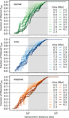Fig. 11

Reduction of the pebble flux through accreting planets. Each line shows the pebble flux in a given heliocentric distance bin at a given time averaged over all simulations for an initial configuration of planetesimals. The panels are as follows: narrow rings (top), wide rings (middle), and high-mass wide rings (bottom). The initial location of the planetesimals (grey area) and the 50 and 80% reduction levels (dashed lines) are shown for reference.

4 Discussion

4.1 Model limitations

4.1.1 Pebble accretion model

Pebble accretion depends significantly on the chosen model for the protoplanetary disc because the scale height of the disc is an important parameter affecting the mass accretion rates of the embryos. The scale height is directly linked to the temperature profile of the disc, which we assumed here to be set by stellar irradiation and is a valid assumption for the outer parts of the disc. However, including accretional heating may have a significant influence on suppressing pebble accretion in the inner part of disc, which may become important for the inwards migrating embryos (Danti et al. 2025).

Pebble accretion depends on the size of the pebbles (Lyra et al. 2023). However, we do not include coagulation or fragmentation in our model to obtain the full size distribution of pebbles and instead use a single representative size given by the limiting cases in Sect. 2.2.1. We assume that upon reaching pebble isolation mass, a planet cuts off the pebble flux, whereas studies of dust growth and transport through planet-induced gaps shows that small dust grains may leak through the gap (Stammler et al. 2023). However, planets that reach pebble isolation mass in our simulations typically originate close to the inner edge of the initial planetesimal distribution or migrate inwards by type-I migration and therefore do not affect growth by pebble accretion in the outer disc.

4.1.2 Gas accretion

The gas accretion prescription chosen in our work is simplified. While the first stage of Kelvin-Helmholtz contraction is a well-established concept (Ikoma et al. 2000), the second stage of runaway gas accretion is merely a power-law fit to numerical simulations (Lambrechts et al. 2019a) that mimics the actual amount of gas entering the Hill sphere of the planet that is accreted. Compared to more detailed prescriptions where the gas accretion rate is regulated by the gap opened by the planet (Tanigawa & Tanaka 2016; Ida et al. 2018), our prescription results in higher gas accretion rates. Consequently, the transition from fast type-I to slower type-II migration occurs earlier in our simulations, which may explain why the gas giants in our simulations remain outside 1 AU compared to previous work (e.g. Bitsch et al. 2019; Lau et al. 2024, and discussion in Sect. 4.2).

4.1.3 Numerical limitation

The GPU-accelerated N-body methods allow significantly more fully interacting bodies to be included in planet formation simulations compared to conventional CPU-based methods. In our nominal simulations, we included around 4000 fully interacting bodies ranging from planetesimals of a few hundred kilometres to approximately 0.1 M_⊕ embryos for the most massive bodies. With this setup, the nebular phase of 4.1 Myr takes a few days to complete and the gas-free phase up to a week. Including more bodies, such as in the high-mass runs with approximately 40 000 bodies, the computational time increases drastically to weeks, even though only ~4000 bodies are fully interacting and the rest are treated as test particles. The most time-consuming part in our simulations is the reduction of the pebble flux, which requires sorting of all pebble accreting bodies in the simulation. We leave an optimisation of this issue to future work.

4.2 Comparison with previous work

Previous N-body work on planet formation by pebble accretion focused on growth of a limited number of embryos to study the effect of disc parameters, pebble flux, or pebble accretion models on the final configuration of planets. Other studies focused specifically on understanding the formation of the giant planets in the Solar System and consequences on for example, terrestrial planet formation or mixing of asteroidal material.

Levison et al. (2015) pioneered the use of N-body simulations of pebble accretion to study the growth of gas giants in the Solar System. Their model showed the formation of one to four gas giants in the 5-15 AU range. This number and heliocentric distance range is comparable to our study, even though Levison et al. (2015) neglected migration, whereas in our model the gas giants migrate from initially ≳10 AU to their final locations between 3 and 15 AU. This shows that despite differences in initial conditions and model parameters, pebble accretion is a robust mechanism to form giant planets. Furthermore, Levison et al. (2015) pointed out the effect of dynamical excitation of embryos on their growth rates. Excitation slows down growth by increasing the relative velocities between the accreting body and the pebbles, which reduces the pebble accretion efficiency, and by increasing the inclination of the embryos, which leads to reduced accretion efficiency because the embryos spend a significant amount of time above or below the pebble scale height. We see both effects in our simulations as well.

Bitsch et al. (2019) use N-body simulations of pebble accretion to explore under which conditions embryos grow to gas giants. They present simulations with 60 embryos in the mass range 0.005-O.015 M_⊕ distributed between 10 and 40 AU, which is similar to our initial configuration, even though we used a full mass distribution of planetesimals instead of embryos. Their scaling factor S_peb = 2.5 for the pebble surface density corresponds to a total pebble mass of ~175 M_⊕ drifting through the gas disc during its lifetime of 3 Myr. In our simulations, the total mass of pebbles integrated from 0.3 to 4.1 Myr is ~ 163 M_⊕, which is comparable. For this pebble flux, Bitsch et al. (2019) observe that only embryos located around 10 AU grow fast enough to eventually accrete gas, but migration is too fast and places those planets close to ~1 AU. Embryos farther out than ~15 AU do not grow quickly enough to reach the threshold for runaway gas accretion to start. For higher pebble fluxes or slower migration speeds, Bitsch et al. (2019) show that embryos grow fast enough to initiate gas accretion and migrate sufficiently slow to remain outside 1 AU.

Raorane et al. (2024) explore the formation of ice and gas giant planets in the Solar System with N-body simulations of pebble accretion. On average, Raorane et al. (2024) form 1.7 planets ≳10 M_⊕ with an average multiplicity of 2.5. This is broadly consistent with our simulations. Furthermore, Raorane et al. (2024) find that ice-giant analogues are rare and that the majority of giant planets exceeds Saturn in mass. Also this is consistent with our simulations where we see a similar trend.

Matsumura et al. (2017) and Matsumura et al. (2021) perform global N -body simulations of pebble accretion to study the influence of various disc parameters, such as dissipation timescale, disc mass and metallicity, on the formed planets. They run 240 simulations for different parameters in which they follow the growth and dynamics of 10 cores with initial mass of 10⁻² M_⊕ distributed over 0.5-15 AU. Matsumura et al. (2021) successfully reproduce the overall distribution trends of semimajor axis, eccentricity, and mass of extrasolar giant planets. Similar to results presented here, they point out that the formation of gas giants is common when the core growth time is shorter than the gas disc dissipation time, else lower-mass ice giants form (Lambrechts & Johansen 2014).

Lau et al. (2024) study planet formation starting from planetesimals using N-body simulations in a similar fashion as in this work. They confirm that dynamical excitation suppresses pebble accretion because encounter times between pebbles and the accreting body become short (Levison et al. 2015). We see the same effect in our simulations where growth by pebble accretion of bodies in the ~10⁻³−1 M_⊕ is suppressed in the dynamically more excited narrow ring runs compared to the dynamically colder wide ring runs. Furthermore, Lau et al. (2024) find that typically one to two gas giants and one to two ice giants form in their simulations outside ~6 AU if migration is not included. However, with migration, massive cores migrate out of their simulation domain before gas accretion could set in resulting in no giant planets. Lau et al. (2024) use a different prescription for gas accretion, planet-disc interactions, and the transition mass to gap-induced type-II migration (Ida et al. 2018). Our gas accretion prescription (Lambrechts et al. 2019a) has higher gas accretion rates, and consequently gas giants transition earlier from fast type-I to slow type-II migration, thus preventing the giant planets from being lost to the inner disc.

4.3 Implications for cold giant exoplanets

It is outside the scope of this work to perform population synthesis and do a statistical comparison to the exoplanet census, which would require a substantially larger simulation suit to explore the effects of disc diversity and to trace stochastic variability (Matsumura et al. 2021). Instead, we briefly comment on some general findings.

Firstly, in systems where gas giants form, we find that they typically orbit between ~3 and ~ 10 AU, and not outside of 20 AU (see Figs. 9). This appears to be broadly in line with an inferred turn over in giant plant occurrence rates at wider orbits outside of ~5AU (Fulton et al. 2021) and the low occurrence of super-Jupiters outside of 20 AU, as inferred from direct imaging surveys (Bowler & Nielsen 2018; Vigan et al. 2021). We also find that, in general, giant planets form in multiples, which appears consistent with inferred giant exoplanet multiplicities (Rosenthal et al. 2024). However, the number of specifically gas giants does not frequently exceed two regardless of initial distribution and initial total mass of planetesimals.

Finally, we briefly comment on the low eccentricities of the giant planets in our simulations, that are typically low and comparable to the eccentricities of the giant planets in the Solar System with e≲0.1 (see Fig. 6). In contrast, the eccentricities of observed exoplanets are typically high (≳0.1), which may be attributed to planet-planet scattering or planet-disc interactions (e.g. Dawson & Murray-Clay 2013; Buchhave et al. 2018; Bitsch et al. 2020). The here obtained eccentricities may depend on the employed eccentricity damping prescription, as explored in Bitsch et al. (2020), and would benefit from explicit hydrodynamical modelling (Griveaud et al. 2024).

4.4 Implications for inner planets

We investigated the formation of planets in the outer disc, starting with planets spread out between 10-50 AU. The reduction of the pebble flux through concurrently accreting embryos, can reduce the pebble flux interior to 10 AU by up to 40% within the first Myr of evolution, depending on the total initial mass of planetesimals. This may have implications for the inner disc, where terrestrial planets form (Lambrechts et al. 2019b). Danti et al. (2025) show that the reduction of the pebble flux by an outer planet alone is typically not sufficient to suppress the growth of inner embryos, unless the inner disc is also strongly heated by accretion heating in the midplane, which increases the gas scale height and suppresses inside-out pebble accretion (Chachan & Lee 2023; Yap & Batygin 2024).

4.5 Scattered disc of not-so-minor bodies

Our simulations show the generic production of a scattered disc of planetesimals and embryos originating from the giantplanet-forming zone. These bodies, with semi-major axis up to 100-200 AU, have a wide mass distribution: from planetesimals originating from the low-mass end of the primordial planetesimal distribution, to Pluto-sized embryos, and onwards to a lower number of planets exceeding the Earth in mass that underwent pebble accretion (Fig. 12). Such discs may be connected to frequently observed debris discs around young stars. The inferred debris and dust production rates are difficult to generate though self-stirring without exceeding the solid mass reservoir of typical protoplanetary disc (Krivov & Wyatt 2021). It has therefore been suggested that the required stirring rates could be connected to the presence of nearby planets (Mustill & Wyatt 2009; Muñoz-Gutiérrez et al. 2023; Costa et al. 2024). Recent observations support at least some of these discs to host a scattered population of bodies: HR 8799 (Geiler et al. 2019), β Pictoris (Matrà et al. 2019), and TWA 7 (Lagrange et al. 2025). The presence of massive embryos in the scattered disc may be a key ingredient to explain debris disc collision rates (Costa et al. 2024).

Although our simulations should not be seen in the context of studies exploring the origin and dynamical sculpting of the Kuiper belt, the natural outcome of a wide mass distribution of scattered objects does support recent explorations that invoke the presence of a substantial population of Pluto-mass objects (Nesvornÿ et al. 2016), potentially more massive objects (Huang et al. 2022), and opens the avenue to implant objects in the Earth-to-ice giant mass regime (Batygin et al. 2019). Since our simulations only trace the initial planetesimal population, making a direct comparison to the Kuiper belt is challenging. Moreover, to assess whether our generic initial conditions could naturally lead to a true outer Solar-System analogue, we would require a larger suite of simulations to trace Solar-System-like dynamical instabilities among giant planets (Gomes et al. 2005; Tsiganis et al. 2005; Morbidelli 2010; Griveaud et al. 2024). However, while the dynamically hot population and the scattered disc were implanted by scattering (Duncan & Levison 1997; Levison et al. 2008; Nesvornÿ et al. 2016), the cold classical Kuiper belt binaries are evidence for in situ planetesimal formation by streaming instability (Nesvornÿ et al. 2019), possibly formed late in the evolution of the gas disc (Carrera et al. 2017; Ercolano et al. 2017; Lau et al. 2025).

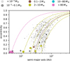Fig. 12

Distribution of planetesimals at 100 Myr for run n05. We show the eccentricity curves where perihelion equals the semi-major axis of the corresponding planets (dashed lines) for reference. The symbol size scales with the mass of the body as ∝m^1/3 and planets ≥ 1 M_⊕ are marked as solid circles.

5 Conclusion

In this work, we have conducted GPU-accelerated N-body simulations of planet formation with pebble accretion using GENGA (Grimm & Stadel 2014; Grimm et al. 2022). We placed the location of our study in the giant-planet formation region between 10 and 50 AU. Starting with a streaming instability inspired initial mass distribution of planetesimals, we simulated 4.1 Myr of evolution in the nebular phase and extended the simulations to 100 Myr in the gas-free phase. We tested two scenarios for the initial radial distribution of planetesimals. In the narrow ring runs, planetesimals were distributed in localised narrow rings between 10 and 50 AU, where each ring had the typical width of a streaming instability filament. In the wide ring runs, the planetesimals were distributed such that the rings connect to represent a more spatially uniform distribution of bodies. In each case, we used a total mass of 1 M_⊕ in planetesimals. For comparison, we also conducted a set of wide ring simulations where we used a ten times higher total mass of planetesimals of 10 M_⊕. Our main findings are summarised as follows.

The initial spatial distribution of planetesimals does not significantly affect the final outcome of our simulations. Starting with narrow rings, scattering and diffusion of planetesimals efficiently redistributes these bodies within the first megayear. In this sense, planetary architectures do not retain a memory of the initial planetesimal distribution.
The qualitative evolution and the final outcome of the narrow and wide ring runs are similar. We consistently find that one to two gas giants form, paired with a handful of icy planets exceeding two Earth masses (Fig. 10).
The initial total mass of planetesimals does not significantly affect the number of planets that form with masses ≳1-2 M_⊕. Reduction of the pebble flux by a high number of concurrently accreting bodies results in a self-regulated growth. This counteracts the expected higher number of planets due to the increased number of seeds resulting in the formation of a similar number of gas giants in the high-mass wide ring simulations with initially 10 M_⊕ of planetesimals compared to the nominal runs with initially only 1 M_⊕.
Our simulations argue that the formation of a scattered disc of planetesimals outside of ~20 AU, with planets with masses ≳0.1 M_⊕ embedded in it, is a natural outcome of giant-planet core formation.
Giant impacts between planetary cores generally appear to be rare in the first 100 Myr.

Acknowledgements

S.L. and M.L. acknowledge this work is funded by the European Research Council (ERC Starting Grant 101041466-EXODOSS). The Tycho supercomputer hosted at the SCIENCE HPC center at the University of Copenhagen was used for supporting this work. We thank Simon Grimm for helpful discussions during the preparation of this work. We thank the anonymous referee for the constructive report that helped to improve the quality of this manuscript.

References

Abod, C. P., Simon, J. B., Li, R., et al. 2019, ApJ, 883, 192 [Google Scholar]
Andrews, S. M. 2020, ARA&A, 58, 483 [Google Scholar]
Appelgren, J., Lambrechts, M., & van der Marel, N. 2023, A&A, 673, A139 [NASA ADS] [CrossRef] [EDP Sciences] [Google Scholar]
Appelgren, J., Johansen, A., Lambrechts, M., et al. 2025, A&A, 694, A311 [NASA ADS] [CrossRef] [EDP Sciences] [Google Scholar]
Batygin, K., Adams, F. C., Brown, M. E., & Becker, J. C. 2019, Phys. Rep., 805, 1 [NASA ADS] [CrossRef] [Google Scholar]
Birnstiel, T., Klahr, H., & Ercolano, B. 2012, A&A, 539, A148 [NASA ADS] [CrossRef] [EDP Sciences] [Google Scholar]
Bitsch, B., Lambrechts, M., & Johansen, A. 2015, A&A, 582, A112 [NASA ADS] [CrossRef] [EDP Sciences] [Google Scholar]
Bitsch, B., Morbidelli, A., Johansen, A., et al. 2018, A&A, 612, A30 [NASA ADS] [CrossRef] [EDP Sciences] [Google Scholar]
Bitsch, B., Izidoro, A., Johansen, A., et al. 2019, A&A, 623, A88 [NASA ADS] [CrossRef] [EDP Sciences] [Google Scholar]
Bitsch, B., Trifonov, T., & Izidoro, A. 2020, A&A, 643, A66 [EDP Sciences] [Google Scholar]
Blum, J., & Wurm, G. 2008, ARA&A, 46, 21 [CrossRef] [Google Scholar]
Boué, G., & Laskar, J. 2010, ApJ, 712, L44 [CrossRef] [Google Scholar]
Bowler, B. P., & Nielsen, E. L. 2018, in Handbook of Exoplanets, eds. H. J. Deeg, & J. A. Belmonte (Berlin: Springer), 155 [Google Scholar]
Brasser, R., & Mojzsis, S. J. 2020, Nat. Astron., 4, 492 [NASA ADS] [CrossRef] [Google Scholar]
Buchhave, L. A., Bitsch, B., Johansen, A., et al. 2018, ApJ, 856, 37 [Google Scholar]
Canup, R. M. 2004, ARA&A, 42, 441 [Google Scholar]
Carrera, D., Gorti, U., Johansen, A., & Davies, M. B. 2017, ApJ, 839, 16 [Google Scholar]
Chachan, Y., & Lee, E. J. 2023, ApJ, 952, L20 [NASA ADS] [CrossRef] [Google Scholar]
Chambers, J. E. 2009, ApJ, 705, 1206 [NASA ADS] [CrossRef] [Google Scholar]
Coleman, G. A. L., & Nelson, R. P. 2014, MNRAS, 445, 479 [Google Scholar]
Coleman, G. A. L., & Nelson, R. P. 2016, MNRAS, 460, 2779 [NASA ADS] [CrossRef] [Google Scholar]
Costa, T., Pearce, T. D., & Krivov, A. V. 2024, MNRAS, 527, 7317 [Google Scholar]
Cresswell, P., & Nelson, R. P. 2008, A&A, 482, 677 [NASA ADS] [CrossRef] [EDP Sciences] [Google Scholar]
D’Angelo, G., & Lubow, S. H. 2010, ApJ, 724, 730 [Google Scholar]
Danti, C., Lambrechts, M., & Lorek, S. 2025, A&A, 700, A132 [NASA ADS] [CrossRef] [EDP Sciences] [Google Scholar]
Dawson, R. I., & Murray-Clay, R. A. 2013, ApJ, 767, L24 [Google Scholar]
Drążkowska, J., Stammler, S. M., & Birnstiel, T. 2021, A&A, 647, A15 [Google Scholar]
Duncan, M. J., & Levison, H. F. 1997, Science, 276, 1670 [Google Scholar]
Ercolano, B., Jennings, J., Rosotti, G., & Birnstiel, T. 2017, MNRAS, 472, 4117 [NASA ADS] [CrossRef] [Google Scholar]
Esteves, L., Izidoro, A., & Winter, O. C. 2025, Icarus, 429, 116428 [Google Scholar]
Fulton, B. J., Rosenthal, L. J., Hirsch, L. A., et al. 2021, ApJS, 255, 14 [NASA ADS] [CrossRef] [Google Scholar]
Geiler, F., Krivov, A. V., Booth, M., & Löhne, T. 2019, MNRAS, 483, 332 [NASA ADS] [CrossRef] [Google Scholar]
Gerbig, K., & Li, R. 2023, ApJ, 949, 81 [NASA ADS] [CrossRef] [Google Scholar]
Gerbig, K., Murray-Clay, R. A., Klahr, H., & Baehr, H. 2020, ApJ, 895, 91 [CrossRef] [Google Scholar]
Gomes, R., Levison, H. F., Tsiganis, K., & Morbidelli, A. 2005, Nature, 435, 466 [Google Scholar]
Grimm, S. L., & Stadel, J. G. 2014, ApJ, 796, 23 [NASA ADS] [CrossRef] [Google Scholar]
Grimm, S. L., Stadel, J. G., Brasser, R., Meier, M. M. M., & Mordasini, C. 2022, ApJ, 932, 124 [NASA ADS] [CrossRef] [Google Scholar]
Griveaud, P., Crida, A., Petit, A. C., Lega, E., & Morbidelli, A. 2024, A&A, 688, A202 [NASA ADS] [CrossRef] [EDP Sciences] [Google Scholar]
Gundlach, B., & Blum, J. 2015, ApJ, 798, 34 [Google Scholar]
Gundlach, B., Schmidt, K. P., Kreuzig, C., et al. 2018, MNRAS, 479, 1273 [NASA ADS] [CrossRef] [Google Scholar]
Gurrutxaga, N., Johansen, A., Lambrechts, M., & Appelgren, J. 2024, A&A, 682, A43 [NASA ADS] [CrossRef] [EDP Sciences] [Google Scholar]
Hartmann, L., Herczeg, G., & Calvet, N. 2016, ARA&A, 54, 135 [Google Scholar]
Huang, Y., Gladman, B., Beaudoin, M., & Zhang, K. 2022, ApJ, 938, L23 [Google Scholar]
Ida, S., & Makino, J. 1992, Icarus, 98, 28 [NASA ADS] [CrossRef] [Google Scholar]
Ida, S., Guillot, T., & Morbidelli, A. 2016, A&A, 591, A72 [NASA ADS] [CrossRef] [EDP Sciences] [Google Scholar]
Ida, S., Tanaka, H., Johansen, A., Kanagawa, K. D., & Tanigawa, T. 2018, ApJ, 864, 77 [NASA ADS] [CrossRef] [Google Scholar]
Ikoma, M., Nakazawa, K., & Emori, H. 2000, ApJ, 537, 1013 [NASA ADS] [CrossRef] [Google Scholar]
Izidoro, A., Morbidelli, A., Raymond, S. N., Hersant, F., & Pierens, A. 2015, A&A, 582, A99 [NASA ADS] [CrossRef] [EDP Sciences] [Google Scholar]
Izidoro, A., Dasgupta, R., Raymond, S. N., et al. 2022, Nat. Astron., 6, 357 [NASA ADS] [CrossRef] [Google Scholar]
Jiang, H., & Ormel, C. W. 2023, MNRAS, 518, 3877 [Google Scholar]
Johansen, A., & Bitsch, B. 2019, A&A, 631, A70 [NASA ADS] [CrossRef] [EDP Sciences] [Google Scholar]
Johansen, A., Oishi, J. S., Mac Low, M.-M., et al. 2007, Nature, 448, 1022 [Google Scholar]
Johansen, A., Blum, J., Tanaka, H., et al. 2014, in Protostars and Planets VI, eds. H. Beuther, R. S. Klessen, C. P. Dullemond, & T. Henning (Tucson: University if Arizona Press), 547 [Google Scholar]
Johansen, A., Mac Low, M.-M., Lacerda, P., & Bizzarro, M. 2015, Sci. Adv., 1, 1500109 [CrossRef] [Google Scholar]
Johansen, A., Ida, S., & Brasser, R. 2019, A&A, 622, A202 [NASA ADS] [CrossRef] [EDP Sciences] [Google Scholar]
Kanagawa, K. D., Tanaka, H., & Szuszkiewicz, E. 2018, ApJ, 861, 140 [Google Scholar]
Kavelaars, J. J., Petit, J.-M., Gladman, B., et al. 2021, ApJ, 920, L28 [NASA ADS] [CrossRef] [Google Scholar]
Kegerreis, J. A., Teodoro, L. F. A., Eke, V. R., et al. 2018, ApJ, 861, 52 [NASA ADS] [CrossRef] [Google Scholar]
Kimura, H., Wada, K., Kobayashi, H., et al. 2020, MNRAS, 498, 1801 [Google Scholar]
Krivov, A. V., & Wyatt, M. C. 2021, MNRAS, 500, 718 [Google Scholar]
Lagrange, A.-M., Wilkinson, C., Mâlin, M., et al. 2025, Nature, 642, 905 [Google Scholar]
Lambrechts, M., & Johansen, A. 2012, A&A, 544, A32 [NASA ADS] [CrossRef] [EDP Sciences] [Google Scholar]
Lambrechts, M., & Johansen, A. 2014, A&A, 572, A107 [NASA ADS] [CrossRef] [EDP Sciences] [Google Scholar]
Lambrechts, M., Johansen, A., & Morbidelli, A. 2014, A&A, 572, A35 [NASA ADS] [CrossRef] [EDP Sciences] [Google Scholar]
Lambrechts, M., Lega, E., Nelson, R. P., Crida, A., & Morbidelli, A. 2019a, A&A, 630, A82 [NASA ADS] [CrossRef] [EDP Sciences] [Google Scholar]
Lambrechts, M., Morbidelli, A., Jacobson, S. A., et al. 2019b, A&A, 627, A83 [NASA ADS] [CrossRef] [EDP Sciences] [Google Scholar]
Lau, T. C. H., Drążkowska, J., Stammler, S. M., Birnstiel, T., & Dullemond, C. P. 2022, A&A, 668, A170 [NASA ADS] [CrossRef] [EDP Sciences] [Google Scholar]
Lau, T. C. H., Lee, M. H., Brasser, R., & Matsumura, S. 2024, A&A, 683, A204 [NASA ADS] [CrossRef] [EDP Sciences] [Google Scholar]
Lau, T. C. H., Birnstiel, T., Stammler, S. M., & Drążkowska, J. 2025, ApJ, 994, 74 [Google Scholar]
Levison, H. F., Morbidelli, A., Van Laerhoven, C., Gomes, R., & Tsiganis, K. 2008, Icarus, 196, 258 [Google Scholar]
Levison, H. F., Thommes, E., & Duncan, M. J. 2010, AJ, 139, 1297 [NASA ADS] [CrossRef] [Google Scholar]
Levison, H. F., Kretke, K. A., & Duncan, M. J. 2015, Nature, 524, 322 [CrossRef] [Google Scholar]
Li, R., Youdin, A. N., & Simon, J. B. 2018, ApJ, 862, 14 [NASA ADS] [CrossRef] [Google Scholar]
Li, R., Youdin, A. N., & Simon, J. B. 2019, ApJ, 885, 69 [NASA ADS] [CrossRef] [Google Scholar]
Liu, B., Ormel, C. W., & Johansen, A. 2019, A&A, 624, A114 [NASA ADS] [CrossRef] [EDP Sciences] [Google Scholar]
Liu, B., Lambrechts, M., Johansen, A., Pascucci, I., & Henning, T. 2020, A&A, 638, A88 [EDP Sciences] [Google Scholar]
Lorek, S., & Johansen, A. 2022, A&A, 666, A108 [NASA ADS] [CrossRef] [EDP Sciences] [Google Scholar]
Lynden-Bell, D., & Pringle, J. E. 1974, MNRAS, 168, 603 [Google Scholar]
Lyra, W., Johansen, A., Cañas, M. H., & Yang, C.-C. 2023, ApJ, 946, 60 [CrossRef] [Google Scholar]
Matrà, L., Wyatt, M. C., Wilner, D. J., et al. 2019, AJ, 157, 135 [CrossRef] [Google Scholar]
Matsumura, S., Brasser, R., & Ida, S. 2017, A&A, 607, A67 [NASA ADS] [CrossRef] [EDP Sciences] [Google Scholar]
Matsumura, S., Brasser, R., & Ida, S. 2021, A&A, 650, A116 [NASA ADS] [CrossRef] [EDP Sciences] [Google Scholar]
Mayor, M., Marmier, M., Lovis, C., et al. 2011, arXiv e-prints [arXiv:1109.2497] [Google Scholar]
Mizuno, H. 1980, Prog. Theor. Phys., 64, 544 [Google Scholar]
Morbidelli, A. 2010, Comptes Rendus Phys., 11, 651 [Google Scholar]
Morbidelli, A. 2020, A&A, 638, A1 [Google Scholar]
Morbidelli, A., Tsiganis, K., Batygin, K., Crida, A., & Gomes, R. 2012, Icarus, 219, 737 [NASA ADS] [CrossRef] [Google Scholar]
Muñoz-Gutiérrez, M. A., Marshall, J. P., & Peimbert, A. 2023, MNRAS, 520, 3218 [Google Scholar]
Mulders, G. D., Pascucci, I., Apai, D., & Ciesla, F. J. 2018, AJ, 156, 24 [Google Scholar]
Musiolik, G., & Wurm, G. 2019, ApJ, 873, 58 [NASA ADS] [CrossRef] [Google Scholar]
Mustill, A. J., & Wyatt, M. C. 2009, MNRAS, 399, 1403 [NASA ADS] [CrossRef] [Google Scholar]
Nesvornÿ, D., Vokrouhlickÿ, D., & Roig, F. 2016, ApJ, 827, L35 [CrossRef] [Google Scholar]
Nesvornÿ, D., Li, R., Youdin, A. N., Simon, J. B., & Grundy, W. M. 2019, Nat. Astron., 3, 808 [CrossRef] [Google Scholar]
Nielsen, E. L., De Rosa, R. J., Macintosh, B., et al. 2019, AJ, 158, 13 [Google Scholar]
Ohtsuki, K., & Tanaka, H. 2003, Icarus, 162, 47 [NASA ADS] [CrossRef] [Google Scholar]
Oka, A., Nakamoto, T., & Ida, S. 2011, ApJ, 738, 141 [Google Scholar]
Okuzumi, S., Tanaka, H., Kobayashi, H., & Wada, K. 2012, ApJ, 752, 106 [NASA ADS] [CrossRef] [Google Scholar]
Ormel, C. W. 2017, Astrophys. Space Sci. Lib., 445, 197 [NASA ADS] [CrossRef] [Google Scholar]
Ormel, C. W., & Klahr, H. H. 2010, A&A, 520, A43 [NASA ADS] [CrossRef] [EDP Sciences] [Google Scholar]
Pollack, J. B., Hubickyj, O., Bodenheimer, P., et al. 1996, Icarus, 124, 62 [NASA ADS] [CrossRef] [Google Scholar]
Rafikov, R. R. 2004, AJ, 128, 1348 [NASA ADS] [CrossRef] [Google Scholar]
Raorane, A., Brasser, R., Matsumura, S., et al. 2024, Icarus, 421, 116231 [NASA ADS] [CrossRef] [Google Scholar]
Reinhardt, C., Chau, A., Stadel, J., & Helled, R. 2020, MNRAS, 492, 5336 [NASA ADS] [CrossRef] [Google Scholar]
Rosenthal, L. J., Fulton, B. J., Hirsch, L. A., et al. 2021, ApJS, 255, 8 [NASA ADS] [CrossRef] [Google Scholar]
Rosenthal, L. J., Howard, A. W., Knutson, H. A., & Fulton, B. J. 2024, ApJS, 270, 1 [NASA ADS] [CrossRef] [Google Scholar]
Saillenfest, M., Rogoszinski, Z., Lari, G., et al. 2022, A&A, 668, A108 [NASA ADS] [CrossRef] [EDP Sciences] [Google Scholar]
Savvidou, S., & Bitsch, B. 2023, A&A, 679, A42 [NASA ADS] [CrossRef] [EDP Sciences] [Google Scholar]
Schäfer, U., Yang, C.-C., & Johansen, A. 2017, A&A, 597, A69 [Google Scholar]
Seager, S., Kuchner, M., Hier-Majumder, C. A., & Militzer, B. 2007, ApJ, 669, 1279 [NASA ADS] [CrossRef] [Google Scholar]
Shakura, N. I., & Sunyaev, R. A. 1973, A&A, 500, 33 [NASA ADS] [Google Scholar]
Simon, J. B., Armitage, P. J., Li, R., & Youdin, A. N. 2016, ApJ, 822, 55 [Google Scholar]
Simon, J. B., Blum, J., Birnstiel, T., & Nesvornÿ, D. 2022, arXiv e-prints [arXiv:2212.04509] [Google Scholar]
Stammler, S. M., Lichtenberg, T., Drążkowska, J., & Birnstiel, T. 2023, A&A, 670, L5 [NASA ADS] [CrossRef] [EDP Sciences] [Google Scholar]
Tanaka, H., & Ida, S. 1999, Icarus, 139, 350 [NASA ADS] [CrossRef] [Google Scholar]
Tanaka, H., Ohtsuki, K., & Daisaka, H. 2003, Icarus, 161, 144 [NASA ADS] [CrossRef] [Google Scholar]
Tanaka, H., & Ward, W. R. 2004, ApJ, 602, 388 [Google Scholar]
Tanigawa, T., & Tanaka, H. 2016, ApJ, 823, 48 [NASA ADS] [CrossRef] [Google Scholar]
Thiemens, M. M., Sprung, P., Fonseca, R. O. C., Leitzke, F. P., & Münker, C. 2019, Nat. Geosci., 12, 696 [NASA ADS] [CrossRef] [Google Scholar]
Thommes, E. W., Duncan, M. J., & Levison, H. F. 2003, Icarus, 161, 431 [NASA ADS] [CrossRef] [Google Scholar]
Tsiganis, K., Gomes, R., Morbidelli, A., & Levison, H. F. 2005, Nature, 435, 459 [Google Scholar]
Vigan, A., Fontanive, C., Meyer, M., et al. 2021, A&A, 651, A72 [EDP Sciences] [Google Scholar]
Wada, K., Tanaka, H., Suyama, T., Kimura, H., & Yamamoto, T. 2009, ApJ, 702, 1490 [Google Scholar]
Wang, H., Weiss, B. P., Bai, X.-N., et al. 2017, Science, 355, 623 [NASA ADS] [CrossRef] [Google Scholar]
Weiss, B. P., Bai, X.-N., & Fu, R. R. 2021, Sci. Adv., 7, eaba5967 [NASA ADS] [CrossRef] [Google Scholar]
Wimarsson, J., Liu, B., & Ogihara, M. 2020, MNRAS, 496, 3314 [NASA ADS] [CrossRef] [Google Scholar]
Wyatt, M. 2020, in The Trans-Neptunian Solar System, eds. D. Prialnik, M. A. Barucci, & L. Young (Amsterdam: Elsevier), 351 [Google Scholar]
Yang, C.-C., & Johansen, A. 2014, ApJ, 792, 86 [Google Scholar]
Yang, C. C., Johansen, A., & Carrera, D. 2017, A&A, 606, A80 [NASA ADS] [CrossRef] [EDP Sciences] [Google Scholar]
Yap, T. E., & Batygin, K. 2024, Icarus, 417, 116085 [Google Scholar]
Youdin, A. N., & Goodman, J. 2005, ApJ, 620, 459 [Google Scholar]

All Tables

Table 1

Simulation parameters and values.

In the text

Table 2

Initial ring locations.

In the text

All Figures

	Fig. 1 Pebble flux (solid) and total pebble mass (dashed) drifting through the system over time.
In the text

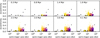	Fig. 4 Same as Fig. 3 but showing the eccentricity and semi-major axis evolution.
In the text

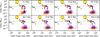	Fig. 5 Same as Fig. 3 but for 4.1-100 Myr.
In the text

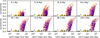	Fig. 6 Same as Fig. 4 but for 4.1-100 Myr.
In the text

	Fig. 7 Collisions as a function of time. We show the projectile-to-target mass ratio for each collision for runs n05 (green) and w05 (blue) from 0.3 to 100 Myr. Each symbol shows a single collision. The nebular phase ends at 4.1 Myr (dashed line). The symbol size scales with the mass of the target as ∝m^1/3.
In the text

	Fig. 8 Mass distribution at 4.1 Myr. We show the average mass distributions for the narrow (green), wide (blue), and high-mass wide (orange) rings at 4.1 Myr (solid lines) with respective standard deviation (shaded area). The initial distributions (dashed lines) are shown for comparison.
In the text

	Fig. 9 Configuration of planets at 4.1 Myr. Each row shows the configuration of planets ≥1 M_⊕ at 4.1 Myr. The runs we show are as follows: narrow ring runs (n05-n10, top), wide ring runs (w03-w08, middle), and high-mass ring runs (m01-m06, bottom). The symbol size scales with the mass of the body as ∝m^1/3, and the colour indicates the mass category.
In the text

	Fig. 10 Number of planets ≥1 M_⊕ at 4.1 Myr. We show the min-max number range (shaded) and the mean number (solid line) of planets formed over all simulations for the narrow (green), wide (blue), and high-mass wide (orange) rings.
In the text

Fig. 11

In the text

	Fig. 12 Distribution of planetesimals at 100 Myr for run n05. We show the eccentricity curves where perihelion equals the semi-major axis of the corresponding planets (dashed lines) for reference. The symbol size scales with the mass of the body as ∝m^1/3 and planets ≥ 1 M_⊕ are marked as solid circles.
In the text

Current usage metrics show cumulative count of Article Views (full-text article views including HTML views, PDF and ePub downloads, according to the available data) and Abstracts Views on Vision4Press platform.

Data correspond to usage on the plateform after 2015. The current usage metrics is available 48-96 hours after online publication and is updated daily on week days.

Initial download of the metrics may take a while.

[R1] Abod, C. P., Simon, J. B., Li, R., et al. 2019, ApJ, 883, 192 [Google Scholar]

[R2] Andrews, S. M. 2020, ARA&A, 58, 483 [Google Scholar]

[R3] Appelgren, J., Lambrechts, M., & van der Marel, N. 2023, A&A, 673, A139 [NASA ADS] [CrossRef] [EDP Sciences] [Google Scholar]

[R4] Appelgren, J., Johansen, A., Lambrechts, M., et al. 2025, A&A, 694, A311 [NASA ADS] [CrossRef] [EDP Sciences] [Google Scholar]

[R5] Batygin, K., Adams, F. C., Brown, M. E., & Becker, J. C. 2019, Phys. Rep., 805, 1 [NASA ADS] [CrossRef] [Google Scholar]

[R6] Birnstiel, T., Klahr, H., & Ercolano, B. 2012, A&A, 539, A148 [NASA ADS] [CrossRef] [EDP Sciences] [Google Scholar]

[R7] Bitsch, B., Lambrechts, M., & Johansen, A. 2015, A&A, 582, A112 [NASA ADS] [CrossRef] [EDP Sciences] [Google Scholar]

[R8] Bitsch, B., Morbidelli, A., Johansen, A., et al. 2018, A&A, 612, A30 [NASA ADS] [CrossRef] [EDP Sciences] [Google Scholar]

[R9] Bitsch, B., Izidoro, A., Johansen, A., et al. 2019, A&A, 623, A88 [NASA ADS] [CrossRef] [EDP Sciences] [Google Scholar]

[R10] Bitsch, B., Trifonov, T., & Izidoro, A. 2020, A&A, 643, A66 [EDP Sciences] [Google Scholar]

[R11] Blum, J., & Wurm, G. 2008, ARA&A, 46, 21 [CrossRef] [Google Scholar]

[R12] Boué, G., & Laskar, J. 2010, ApJ, 712, L44 [CrossRef] [Google Scholar]

[R13] Bowler, B. P., & Nielsen, E. L. 2018, in Handbook of Exoplanets, eds. H. J. Deeg, & J. A. Belmonte (Berlin: Springer), 155 [Google Scholar]

[R14] Brasser, R., & Mojzsis, S. J. 2020, Nat. Astron., 4, 492 [NASA ADS] [CrossRef] [Google Scholar]

[R15] Buchhave, L. A., Bitsch, B., Johansen, A., et al. 2018, ApJ, 856, 37 [Google Scholar]

[R16] Canup, R. M. 2004, ARA&A, 42, 441 [Google Scholar]

[R17] Carrera, D., Gorti, U., Johansen, A., & Davies, M. B. 2017, ApJ, 839, 16 [Google Scholar]

[R18] Chachan, Y., & Lee, E. J. 2023, ApJ, 952, L20 [NASA ADS] [CrossRef] [Google Scholar]

[R19] Chambers, J. E. 2009, ApJ, 705, 1206 [NASA ADS] [CrossRef] [Google Scholar]

[R20] Coleman, G. A. L., & Nelson, R. P. 2014, MNRAS, 445, 479 [Google Scholar]

[R21] Coleman, G. A. L., & Nelson, R. P. 2016, MNRAS, 460, 2779 [NASA ADS] [CrossRef] [Google Scholar]

[R22] Costa, T., Pearce, T. D., & Krivov, A. V. 2024, MNRAS, 527, 7317 [Google Scholar]

[R23] Cresswell, P., & Nelson, R. P. 2008, A&A, 482, 677 [NASA ADS] [CrossRef] [EDP Sciences] [Google Scholar]

[R24] D’Angelo, G., & Lubow, S. H. 2010, ApJ, 724, 730 [Google Scholar]

[R25] Danti, C., Lambrechts, M., & Lorek, S. 2025, A&A, 700, A132 [NASA ADS] [CrossRef] [EDP Sciences] [Google Scholar]

[R26] Dawson, R. I., & Murray-Clay, R. A. 2013, ApJ, 767, L24 [Google Scholar]

[R27] Drążkowska, J., Stammler, S. M., & Birnstiel, T. 2021, A&A, 647, A15 [Google Scholar]

[R28] Duncan, M. J., & Levison, H. F. 1997, Science, 276, 1670 [Google Scholar]

[R29] Ercolano, B., Jennings, J., Rosotti, G., & Birnstiel, T. 2017, MNRAS, 472, 4117 [NASA ADS] [CrossRef] [Google Scholar]

[R30] Esteves, L., Izidoro, A., & Winter, O. C. 2025, Icarus, 429, 116428 [Google Scholar]

[R31] Fulton, B. J., Rosenthal, L. J., Hirsch, L. A., et al. 2021, ApJS, 255, 14 [NASA ADS] [CrossRef] [Google Scholar]

[R32] Geiler, F., Krivov, A. V., Booth, M., & Löhne, T. 2019, MNRAS, 483, 332 [NASA ADS] [CrossRef] [Google Scholar]

[R33] Gerbig, K., & Li, R. 2023, ApJ, 949, 81 [NASA ADS] [CrossRef] [Google Scholar]

[R34] Gerbig, K., Murray-Clay, R. A., Klahr, H., & Baehr, H. 2020, ApJ, 895, 91 [CrossRef] [Google Scholar]

[R35] Gomes, R., Levison, H. F., Tsiganis, K., & Morbidelli, A. 2005, Nature, 435, 466 [Google Scholar]

[R36] Grimm, S. L., & Stadel, J. G. 2014, ApJ, 796, 23 [NASA ADS] [CrossRef] [Google Scholar]

[R37] Grimm, S. L., Stadel, J. G., Brasser, R., Meier, M. M. M., & Mordasini, C. 2022, ApJ, 932, 124 [NASA ADS] [CrossRef] [Google Scholar]

[R38] Griveaud, P., Crida, A., Petit, A. C., Lega, E., & Morbidelli, A. 2024, A&A, 688, A202 [NASA ADS] [CrossRef] [EDP Sciences] [Google Scholar]

[R39] Gundlach, B., & Blum, J. 2015, ApJ, 798, 34 [Google Scholar]

[R40] Gundlach, B., Schmidt, K. P., Kreuzig, C., et al. 2018, MNRAS, 479, 1273 [NASA ADS] [CrossRef] [Google Scholar]

[R41] Gurrutxaga, N., Johansen, A., Lambrechts, M., & Appelgren, J. 2024, A&A, 682, A43 [NASA ADS] [CrossRef] [EDP Sciences] [Google Scholar]

[R42] Hartmann, L., Herczeg, G., & Calvet, N. 2016, ARA&A, 54, 135 [Google Scholar]

[R43] Huang, Y., Gladman, B., Beaudoin, M., & Zhang, K. 2022, ApJ, 938, L23 [Google Scholar]

[R44] Ida, S., & Makino, J. 1992, Icarus, 98, 28 [NASA ADS] [CrossRef] [Google Scholar]

[R45] Ida, S., Guillot, T., & Morbidelli, A. 2016, A&A, 591, A72 [NASA ADS] [CrossRef] [EDP Sciences] [Google Scholar]

[R46] Ida, S., Tanaka, H., Johansen, A., Kanagawa, K. D., & Tanigawa, T. 2018, ApJ, 864, 77 [NASA ADS] [CrossRef] [Google Scholar]

[R47] Ikoma, M., Nakazawa, K., & Emori, H. 2000, ApJ, 537, 1013 [NASA ADS] [CrossRef] [Google Scholar]

[R48] Izidoro, A., Morbidelli, A., Raymond, S. N., Hersant, F., & Pierens, A. 2015, A&A, 582, A99 [NASA ADS] [CrossRef] [EDP Sciences] [Google Scholar]

[R49] Izidoro, A., Dasgupta, R., Raymond, S. N., et al. 2022, Nat. Astron., 6, 357 [NASA ADS] [CrossRef] [Google Scholar]

[R50] Jiang, H., & Ormel, C. W. 2023, MNRAS, 518, 3877 [Google Scholar]

[R51] Johansen, A., & Bitsch, B. 2019, A&A, 631, A70 [NASA ADS] [CrossRef] [EDP Sciences] [Google Scholar]

[R52] Johansen, A., Oishi, J. S., Mac Low, M.-M., et al. 2007, Nature, 448, 1022 [Google Scholar]

[R53] Johansen, A., Blum, J., Tanaka, H., et al. 2014, in Protostars and Planets VI, eds. H. Beuther, R. S. Klessen, C. P. Dullemond, & T. Henning (Tucson: University if Arizona Press), 547 [Google Scholar]

[R54] Johansen, A., Mac Low, M.-M., Lacerda, P., & Bizzarro, M. 2015, Sci. Adv., 1, 1500109 [CrossRef] [Google Scholar]

[R55] Johansen, A., Ida, S., & Brasser, R. 2019, A&A, 622, A202 [NASA ADS] [CrossRef] [EDP Sciences] [Google Scholar]

[R56] Kanagawa, K. D., Tanaka, H., & Szuszkiewicz, E. 2018, ApJ, 861, 140 [Google Scholar]

[R57] Kavelaars, J. J., Petit, J.-M., Gladman, B., et al. 2021, ApJ, 920, L28 [NASA ADS] [CrossRef] [Google Scholar]

[R58] Kegerreis, J. A., Teodoro, L. F. A., Eke, V. R., et al. 2018, ApJ, 861, 52 [NASA ADS] [CrossRef] [Google Scholar]

[R59] Kimura, H., Wada, K., Kobayashi, H., et al. 2020, MNRAS, 498, 1801 [Google Scholar]

[R60] Krivov, A. V., & Wyatt, M. C. 2021, MNRAS, 500, 718 [Google Scholar]

[R61] Lagrange, A.-M., Wilkinson, C., Mâlin, M., et al. 2025, Nature, 642, 905 [Google Scholar]

[R62] Lambrechts, M., & Johansen, A. 2012, A&A, 544, A32 [NASA ADS] [CrossRef] [EDP Sciences] [Google Scholar]

[R63] Lambrechts, M., & Johansen, A. 2014, A&A, 572, A107 [NASA ADS] [CrossRef] [EDP Sciences] [Google Scholar]

[R64] Lambrechts, M., Johansen, A., & Morbidelli, A. 2014, A&A, 572, A35 [NASA ADS] [CrossRef] [EDP Sciences] [Google Scholar]

[R65] Lambrechts, M., Lega, E., Nelson, R. P., Crida, A., & Morbidelli, A. 2019a, A&A, 630, A82 [NASA ADS] [CrossRef] [EDP Sciences] [Google Scholar]

[R66] Lambrechts, M., Morbidelli, A., Jacobson, S. A., et al. 2019b, A&A, 627, A83 [NASA ADS] [CrossRef] [EDP Sciences] [Google Scholar]

[R67] Lau, T. C. H., Drążkowska, J., Stammler, S. M., Birnstiel, T., & Dullemond, C. P. 2022, A&A, 668, A170 [NASA ADS] [CrossRef] [EDP Sciences] [Google Scholar]

[R68] Lau, T. C. H., Lee, M. H., Brasser, R., & Matsumura, S. 2024, A&A, 683, A204 [NASA ADS] [CrossRef] [EDP Sciences] [Google Scholar]

[R69] Lau, T. C. H., Birnstiel, T., Stammler, S. M., & Drążkowska, J. 2025, ApJ, 994, 74 [Google Scholar]

[R70] Levison, H. F., Morbidelli, A., Van Laerhoven, C., Gomes, R., & Tsiganis, K. 2008, Icarus, 196, 258 [Google Scholar]

[R71] Levison, H. F., Thommes, E., & Duncan, M. J. 2010, AJ, 139, 1297 [NASA ADS] [CrossRef] [Google Scholar]

[R72] Levison, H. F., Kretke, K. A., & Duncan, M. J. 2015, Nature, 524, 322 [CrossRef] [Google Scholar]

[R73] Li, R., Youdin, A. N., & Simon, J. B. 2018, ApJ, 862, 14 [NASA ADS] [CrossRef] [Google Scholar]

[R74] Li, R., Youdin, A. N., & Simon, J. B. 2019, ApJ, 885, 69 [NASA ADS] [CrossRef] [Google Scholar]

[R75] Liu, B., Ormel, C. W., & Johansen, A. 2019, A&A, 624, A114 [NASA ADS] [CrossRef] [EDP Sciences] [Google Scholar]

[R76] Liu, B., Lambrechts, M., Johansen, A., Pascucci, I., & Henning, T. 2020, A&A, 638, A88 [EDP Sciences] [Google Scholar]

[R77] Lorek, S., & Johansen, A. 2022, A&A, 666, A108 [NASA ADS] [CrossRef] [EDP Sciences] [Google Scholar]

[R78] Lynden-Bell, D., & Pringle, J. E. 1974, MNRAS, 168, 603 [Google Scholar]

[R79] Lyra, W., Johansen, A., Cañas, M. H., & Yang, C.-C. 2023, ApJ, 946, 60 [CrossRef] [Google Scholar]

[R80] Matrà, L., Wyatt, M. C., Wilner, D. J., et al. 2019, AJ, 157, 135 [CrossRef] [Google Scholar]

[R81] Matsumura, S., Brasser, R., & Ida, S. 2017, A&A, 607, A67 [NASA ADS] [CrossRef] [EDP Sciences] [Google Scholar]

[R82] Matsumura, S., Brasser, R., & Ida, S. 2021, A&A, 650, A116 [NASA ADS] [CrossRef] [EDP Sciences] [Google Scholar]

[R83] Mayor, M., Marmier, M., Lovis, C., et al. 2011, arXiv e-prints [arXiv:1109.2497] [Google Scholar]

[R84] Mizuno, H. 1980, Prog. Theor. Phys., 64, 544 [Google Scholar]

[R85] Morbidelli, A. 2010, Comptes Rendus Phys., 11, 651 [Google Scholar]

[R86] Morbidelli, A. 2020, A&A, 638, A1 [Google Scholar]

[R87] Morbidelli, A., Tsiganis, K., Batygin, K., Crida, A., & Gomes, R. 2012, Icarus, 219, 737 [NASA ADS] [CrossRef] [Google Scholar]

[R88] Muñoz-Gutiérrez, M. A., Marshall, J. P., & Peimbert, A. 2023, MNRAS, 520, 3218 [Google Scholar]

[R89] Mulders, G. D., Pascucci, I., Apai, D., & Ciesla, F. J. 2018, AJ, 156, 24 [Google Scholar]

[R90] Musiolik, G., & Wurm, G. 2019, ApJ, 873, 58 [NASA ADS] [CrossRef] [Google Scholar]

[R91] Mustill, A. J., & Wyatt, M. C. 2009, MNRAS, 399, 1403 [NASA ADS] [CrossRef] [Google Scholar]

[R92] Nesvornÿ, D., Vokrouhlickÿ, D., & Roig, F. 2016, ApJ, 827, L35 [CrossRef] [Google Scholar]

[R93] Nesvornÿ, D., Li, R., Youdin, A. N., Simon, J. B., & Grundy, W. M. 2019, Nat. Astron., 3, 808 [CrossRef] [Google Scholar]

[R94] Nielsen, E. L., De Rosa, R. J., Macintosh, B., et al. 2019, AJ, 158, 13 [Google Scholar]

[R95] Ohtsuki, K., & Tanaka, H. 2003, Icarus, 162, 47 [NASA ADS] [CrossRef] [Google Scholar]

[R96] Oka, A., Nakamoto, T., & Ida, S. 2011, ApJ, 738, 141 [Google Scholar]

[R97] Okuzumi, S., Tanaka, H., Kobayashi, H., & Wada, K. 2012, ApJ, 752, 106 [NASA ADS] [CrossRef] [Google Scholar]

[R98] Ormel, C. W. 2017, Astrophys. Space Sci. Lib., 445, 197 [NASA ADS] [CrossRef] [Google Scholar]

[R99] Ormel, C. W., & Klahr, H. H. 2010, A&A, 520, A43 [NASA ADS] [CrossRef] [EDP Sciences] [Google Scholar]

[R100] Pollack, J. B., Hubickyj, O., Bodenheimer, P., et al. 1996, Icarus, 124, 62 [NASA ADS] [CrossRef] [Google Scholar]

[R101] Rafikov, R. R. 2004, AJ, 128, 1348 [NASA ADS] [CrossRef] [Google Scholar]

[R102] Raorane, A., Brasser, R., Matsumura, S., et al. 2024, Icarus, 421, 116231 [NASA ADS] [CrossRef] [Google Scholar]

[R103] Reinhardt, C., Chau, A., Stadel, J., & Helled, R. 2020, MNRAS, 492, 5336 [NASA ADS] [CrossRef] [Google Scholar]

[R104] Rosenthal, L. J., Fulton, B. J., Hirsch, L. A., et al. 2021, ApJS, 255, 8 [NASA ADS] [CrossRef] [Google Scholar]

[R105] Rosenthal, L. J., Howard, A. W., Knutson, H. A., & Fulton, B. J. 2024, ApJS, 270, 1 [NASA ADS] [CrossRef] [Google Scholar]

[R106] Saillenfest, M., Rogoszinski, Z., Lari, G., et al. 2022, A&A, 668, A108 [NASA ADS] [CrossRef] [EDP Sciences] [Google Scholar]

[R107] Savvidou, S., & Bitsch, B. 2023, A&A, 679, A42 [NASA ADS] [CrossRef] [EDP Sciences] [Google Scholar]

[R108] Schäfer, U., Yang, C.-C., & Johansen, A. 2017, A&A, 597, A69 [Google Scholar]

[R109] Seager, S., Kuchner, M., Hier-Majumder, C. A., & Militzer, B. 2007, ApJ, 669, 1279 [NASA ADS] [CrossRef] [Google Scholar]

[R110] Shakura, N. I., & Sunyaev, R. A. 1973, A&A, 500, 33 [NASA ADS] [Google Scholar]

[R111] Simon, J. B., Armitage, P. J., Li, R., & Youdin, A. N. 2016, ApJ, 822, 55 [Google Scholar]

[R112] Simon, J. B., Blum, J., Birnstiel, T., & Nesvornÿ, D. 2022, arXiv e-prints [arXiv:2212.04509] [Google Scholar]

[R113] Stammler, S. M., Lichtenberg, T., Drążkowska, J., & Birnstiel, T. 2023, A&A, 670, L5 [NASA ADS] [CrossRef] [EDP Sciences] [Google Scholar]

[R114] Tanaka, H., & Ida, S. 1999, Icarus, 139, 350 [NASA ADS] [CrossRef] [Google Scholar]

[R115] Tanaka, H., Ohtsuki, K., & Daisaka, H. 2003, Icarus, 161, 144 [NASA ADS] [CrossRef] [Google Scholar]

[R116] Tanaka, H., & Ward, W. R. 2004, ApJ, 602, 388 [Google Scholar]

[R117] Tanigawa, T., & Tanaka, H. 2016, ApJ, 823, 48 [NASA ADS] [CrossRef] [Google Scholar]

[R118] Thiemens, M. M., Sprung, P., Fonseca, R. O. C., Leitzke, F. P., & Münker, C. 2019, Nat. Geosci., 12, 696 [NASA ADS] [CrossRef] [Google Scholar]

[R119] Thommes, E. W., Duncan, M. J., & Levison, H. F. 2003, Icarus, 161, 431 [NASA ADS] [CrossRef] [Google Scholar]

[R120] Tsiganis, K., Gomes, R., Morbidelli, A., & Levison, H. F. 2005, Nature, 435, 459 [Google Scholar]

[R121] Vigan, A., Fontanive, C., Meyer, M., et al. 2021, A&A, 651, A72 [EDP Sciences] [Google Scholar]

[R122] Wada, K., Tanaka, H., Suyama, T., Kimura, H., & Yamamoto, T. 2009, ApJ, 702, 1490 [Google Scholar]

[R123] Wang, H., Weiss, B. P., Bai, X.-N., et al. 2017, Science, 355, 623 [NASA ADS] [CrossRef] [Google Scholar]

[R124] Weiss, B. P., Bai, X.-N., & Fu, R. R. 2021, Sci. Adv., 7, eaba5967 [NASA ADS] [CrossRef] [Google Scholar]

[R125] Wimarsson, J., Liu, B., & Ogihara, M. 2020, MNRAS, 496, 3314 [NASA ADS] [CrossRef] [Google Scholar]

[R126] Wyatt, M. 2020, in The Trans-Neptunian Solar System, eds. D. Prialnik, M. A. Barucci, & L. Young (Amsterdam: Elsevier), 351 [Google Scholar]

[R127] Yang, C.-C., & Johansen, A. 2014, ApJ, 792, 86 [Google Scholar]

[R128] Yang, C. C., Johansen, A., & Carrera, D. 2017, A&A, 606, A80 [NASA ADS] [CrossRef] [EDP Sciences] [Google Scholar]

[R129] Yap, T. E., & Batygin, K. 2024, Icarus, 417, 116085 [Google Scholar]

[R130] Youdin, A. N., & Goodman, J. 2005, ApJ, 620, 459 [Google Scholar]