| Issue |
A&A
Volume 708, April 2026
|
|
|---|---|---|
| Article Number | A127 | |
| Number of page(s) | 15 | |
| Section | Cosmology (including clusters of galaxies) | |
| DOI | https://doi.org/10.1051/0004-6361/202556689 | |
| Published online | 31 March 2026 | |
Optimising the sample selection for photometric galaxy surveys
1
Institute of Space Sciences (ICE, CSIC), Campus UAB, Carrer de Can Magrans s/n, 08193 Barcelona, Spain
2
Institut d’Estudis Espacials de Catalunya (IEEC), Carrer Gran Capitá 2-4, 08034 Barcelona, Spain
3
Institut de Recherche en Astrophysique et Planétologie (IRAP), Université de Toulouse, CNRS, UPS, CNES, 14 Av. Edouard Belin, 31400 Toulouse, France
★ Corresponding author: This email address is being protected from spambots. You need JavaScript enabled to view it.
Received:
31
July
2025
Accepted:
15
December
2025
Abstract
Context. Determining cosmological parameters with high precision, as well as resolving current tensions in their values derived from low- and high-redshift probes, is one of the main objectives of the new generation of cosmological surveys. The combination of complementary probes in terms of parameter degeneracies and systematics is key to achieving these ambitious scientific goals.
Aims. In this context, determining the optimal survey configuration for an analysis that combines galaxy clustering, weak lensing, and galaxy-galaxy lensing, the so-called 3 × 2pt analysis, remains an open problem. In this paper, we present an efficient and flexible end-to-end pipeline to optimise the sample selection for 3x2pt analyses in an automated way.
Methods. Our pipeline is articulated in two main steps: we first consider a self-organising map to determine the photometric redshifts of a simulated galaxy sample. As a proof of method for stage IV surveys, we use samples from the DESC Data Challenge 2 catalogue. This allows us to classify galaxies into tomographic bins based on their colour phenotype clustering. We then explore different redshift-bin edge configurations for weak lensing only as well as 3 × 2pt analyses in a novel way. Our method explores multiple configurations of perturbed redshift-bin edges with respect to the fiducial case in an iterative manner. In particular, we sample tomographic configurations for the source and lens galaxies separately.
Results. We show that using this method we quickly converge on an optimised configuration for different numbers of redshift bins and cosmologies. Our analysis demonstrates that for stage IV surveys an optimal tomographic sample selection can increase the figure of merit of the dark energy (DE) equation of state by a factor of ∼2, comparable to an effective increase in survey area of ∼4 for non-optimal photometric survey analyses.
Key words: gravitational lensing: weak / methods: data analysis / techniques: photometric
© The Authors 2026
 Open Access article, published by EDP Sciences, under the terms of the Creative Commons Attribution License (https://creativecommons.org/licenses/by/4.0), which permits unrestricted use, distribution, and reproduction in any medium, provided the original work is properly cited.
This article is published in open access under the Subscribe to Open model. This email address is being protected from spambots. You need JavaScript enabled to view it. to support open access publication.
1. Introduction
In the current era of precision cosmology, surveys such as Euclid (Euclid Collaboration: Mellier et al. 2025) or the Legacy Survey of Space and Time (LSST; Ivezić et al. 2019) from the Vera C. Rubin observatory are expected to provide data for more than a billion galaxies up to high redshift. In this scenario, the weak lensing (WL) and galaxy clustering (GC) probes, which measure excess correlations in the apparent shear and position of galaxies as a function of angular separation, respectively, will allow for unprecedented insights into the expansion history and growth rate of the large-scale structure (LSS) of the Universe. This will provide a significant improvement in cosmological parameter constraints as well as in the characterisation of dark energy (DE). In addition, recent results from the Dark Energy Spectroscopic Instrument (DESI) collaboration (Abdul Karim et al. 2025) have shown deviations from Λ cold dark matter (CDM) of notable statistical significance in favour of dynamical DE. In light of this, there is increased interest in testing w0waCDM models with galaxy survey probes.
Since the LSS is sensitive to the influence of both dark matter and DE, the statistics of GC and WL allow for a mapping of the distribution of matter through space and time. GC requires some assumptions over the relation between dark and baryonic matter, and can only correctly trace dark matter as long as this relation, encompassed in the galaxy bias parameters, is fully characterised (Desjacques et al. 2018). In contrast, WL is a direct tracer of dark matter. Combining the two probes, as well as galaxy–galaxy lensing (GGL), allows for a more robust analysis method by breaking degeneracies present in individual probes (Salcedo et al. 2020; Tutusaus et al. 2020). Combining the three probes as well as their correlation is what is called 3 × 2 pt analysis, which has been extensively used with current observations (Abbott et al. 2022; Heymans et al. 2021) and will be used for stage IV surveys (Euclid Collaboration: Blanchard et al. 2020; Zuntz et al. 2021; Prince et al. 2025).
Optimising the sample selection for a single probe may not result in the optimal sample selection for a different probe. Moreover, in a realistic 3 × 2 pt analysis the interplay between the different probes and their cross-correlations requires the optimisation to be done for the full set of probes involved. However, direct numerical attempts to find an optimised tomographic redshift bin configuration are hindered by the high computational cost of running a Bayesian inference pipeline at every step of the optimisation.
Several efforts have previously been performed in the literature to optimise the sample selection, some (e.g. Euclid Collaboration: Pocino et al. (2021), Wong et al. (2026)) focussing on comparing equally populated and equal-width tomographic redshift bins, and others (e.g. Kitching et al. 2019; Sipp et al. 2021) presenting more general optimisation methods limited to a lower number of redshift bins with lensing alone. Several methods presented in Zuntz et al. (2021) attempt to improve the tomographic configuration by optimising the classification of galaxies into redshift bins. In this work we follow a different approach whereby we do not limit our exploration to a pre-defined set of possibilities (e.g. equally populated vs equal-width tomographic bins) and in this way we allow for different tomographic configurations to be tested. Nevertheless, we do not perform a completely general study of possible samples either, as that results in an intractable amount of possible configurations (e.g. for more than three tomographic bins a completely brute-force search of the optimal sample selection is already intractable, as is shown in Sipp et al. 2021). Instead, we opt to optimise the tomographic bin edges separately for source and lens galaxy populations in an iterative manner, starting from the equally spaced redshift bin case1. For the proof of method presented in this paper, we performed the optimisation for dynamic DE cosmology, using a tomographic 3 × 2 pt analysis. Our implemented end-to-end pipeline is rather efficient, yielding a feasible computation time to converge into a robust solution (∼1200 CPU hours). Our results show that using this method one can significantly improve the cosmological constraints (up to a factor of 2.5 in some cases) with respect to non-optimal tomographic analyses.
We have created a framework for tomographic optimisation that consists of an algorithm to run a pipeline of cosmological parameter inference based on the Cosmological Survey Inference System (CosmoSIS, Zuntz et al. 2015). We use as input data a photo-z catalogue that we generated based on a simulation. The constraining power for each of the studied samples was obtained using a Fisher matrix forecast technique.
The paper is organised as follows. In Sect. 2 we describe the mock data and the method of obtaining the photo-z catalogue that we used as an input. In Sect. 3 we present the formalism of the 3 × 2pt pipeline as well as the tomographic optimisation algorithm. In Sect. 4 we show the results of the optimisation for two sets of cosmological parameters. In Sect. 5 we discuss our results and compare them against those available in the literature. Finally, in Sect. 6 we present the main conclusions of the analysis.
2. Mock input data
The method of tomographic optimisation introduced in this work requires an input photo-z catalogue. As we describe below, our input mock dataset does not include photo-z, and thus we opted to generate a stage-IV-like photometric galaxy catalogue using a self-organising map (SOM). For this purpose, we estimate photo-z based on each galaxy’s ugrizy-band fluxes using a SOM. The SOM implementation closely follows a similar algorithm presented in Kitching et al. (2019). Instead of using band fluxes directly, we work in colour space, defining the following colours: u − g, g − r, r − i, i − z, and z − y.
2.1. Simulated data
The data that we used comes from the DESC Data Challenge 2 (DESC DC2, Abolfathi et al. 2021), and consists of a simulated galaxy catalogue mimicking a small patch of the expected observations of the future Rubin Observatory. We downloaded our samples using CosmoHub (Tallada et al. 2020; Carretero et al. 2017). DESC DC2 is based on the CosmoDC2 simulation (Korytov et al. 2019), (Abolfathi et al. 2021). It covers ∼440 square degrees with photometric data of galaxies up to redshift 3 in the ugrizy bands. The simulation was created as part of the preparation for LSST (Zuntz et al. 2021; Moskowitz et al. 2023), which is expected to provide an unprecedented amount of astronomical data that will enable scientists to address a wide range of critical questions in observational cosmology, constraining the nature of DE and dark matter and providing a better understanding of how galaxies form.
The DESC DC2 simulation includes several key features that make it an ideal tool with which to study these phenomena. First, it includes a large number of galaxies, modelled using sophisticated algorithms that take into account a wide range of physical processes, such as star formation, gas dynamics, and feedback from supernovae and black holes. Second, the simulation covers a large volume of space, spanning over 440 square degrees on the sky, with a high level of detail and resolution. The CosmoDC2 catalogue is based on the Outer Rim simulation, an N-body halo simulation by Heitmann et al. (2019) that assumes a ΛCDM model with the cosmological parameters being the matter density Ωm = 0.27, the baryonic matter density Ωb = 0.045, the spectral index ns = 0.963, the dimensionless Hubble parameter h = 0.71, and the amplitude of matter fluctuations in spheres of 8 Mpc/hσ8 = 0.8. Since it assumes ΛCDM, the values for the DE equation of state parameters are w0 = −1 and wa = 0. It consists of a 4.225 Gpc3 box with a 10.2403 particles and a resolution of 2.6 × 10⁹ M⊙, producing 101 snapshots from a starting redshift of z = 10 to z = 0.
We assumed the simulation cosmology when performing our analysis, except for the addition of dynamical DE with the w0waCDM model, which included the following dynamical DE modelling with a varying equation of state parameter:
 (1)
(1)
where w0 corresponds to the value of the equation of state parameter today and wa parametrises the variation in the dynamics of DE over redshift (Linder 2003; Chevallier & Polarski 2001). In this context, the optimisation we performed was to minimise the errors around the reference cosmology of the simulated data we used, ΛCDM, across the w0waCDM model parameters.
The catalogue contains the fluxes, positions and shear of the galaxies. We used the colours defined as the differences in magnitude of pairs of fluxes, propagating the flux errors into colour errors. The photo-z estimation for each galaxy was performed using the galaxies’ colour vector and associated error.
2.2. Photo-z estimation
A SOM is essentially a method of reducing the dimensionality of high-dimensional data by projecting it onto a lower-dimensional representation. It consists of a two-dimensional grid map composed of n1 × n2 discrete points called neurons or voxels. Each voxel (j, k) in this grid has an associated m-dimensional weight vector wjk, where the indices jk specify the voxel’s position on the map. In particular, the weights have five dimensions corresponding to the five colour values that each galaxy has. Initially, these weight vectors are set to random values. During the training process, the SOM algorithm iteratively adjusts these weights so that voxels with similar weight vectors become clustered together on the map. This creates a topology whereby galaxies with similar colour phenotypes will be mapped to nearby regions.
Once training is complete, individual galaxies are assigned to specific voxels based on the best match between the galaxy’s observed colours and the weight vectors of the voxels, typically using a minimum distance criterion. The photo-z estimation is then performed by assigning to each galaxy a redshift value using the n(z) distribution associated with its matched voxel. The n(z) of a given voxel is composed of the spectroscopic redshift of the training galaxies that were assigned to that voxel. Thus, the SOM reduces the dimensionality of our data and allows for both photo-z estimation and for the possibility of selecting phenotypically similar galaxies based only on their proximity on the map. More details on the specific implementation of the SOM are given in the Appendix A.
2.2.1. Training and photo-z galaxy catalogues
For our training sample, we selected an r-band magnitude-limited (< 24.0) sample in a patch of 4 square degrees, containing ∼105 galaxies. The patch size was selected so that the number of galaxies was similar to the sample used for the training of a SOM in Masters et al. (2015). Our photo-z galaxies were selected by an r-band magnitude cut at < 24.5 leading to a galaxy sample that contains ∼1.3 × 10⁷ photometric galaxies over a patch of 225 square degrees. The magnitude cut for the photometric galaxy sample was chosen to resemble stage IV forecasts (Euclid Collaboration: Pocino et al. 2021). The magnitude cuts of the training sample are optimistic and motivated by the need to achieve a meaningful level of high-redshift galaxies. This is because the ultimate goal of our work is to present a tomographic sample optimisation method for a stage-IV-like photometric galaxy sample and our training galaxy sample was adjusted accordingly. Finally, we also selected galaxies with a true redshift below z = 2 for both catalogues. This is because introducing galaxies above that redshift will worsen the general performance of the SOM without providing an adequate characterisation of those high redshift galaxies. We note, however, that this selection should not limit the general validity of our approach for stage IV experiments, as we cover a redshift range comparable to current or future surveys. We present a quantitative analysis of the performance of the photo-z estimation using the SOM in Sect. 2.2.2.
2.2.2. Performance evaluation
We evaluated the performance of the SOM in properly assigning photo-z to galaxies based on their colours. Since the data that we used were generated with a simulation, we knew the true redshift of the galaxies in the catalogue. This allowed for a precise characterisation of the performance of the photo-z estimation method. We also compared the distributions of the true redshift and of the SOM-estimated photo-z in the top panel of Fig. 1, where the photo-z distribution closely matches the original. The number of galaxies at high redshift in the training sample is low, leading to poorer photo-z for high-redshift galaxies. The SOM photo-zn(z) resembles the true redshift n(z) nonetheless, even at high redshift.
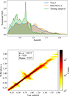 |
Fig. 1. SOM performance evaluation. The top panel shows the normalised distributions of the true redshift of galaxies from the simulated catalogue (blue), of the estimated photo-z generated with the SOM (orange), and of the sample used to train the SOM (green). The bottom panel shows the performance of the SOM in the estimation of the photo-z of galaxies. |
In the bottom panel of Fig. 1, we evaluate the performance of the SOM through the use of three metrics: the outlier rate, μ0.15, the bias, bz, and the normalised median absolute deviation, σNMAD. These metrics together provide an assessment of the accuracy of the photo-z estimates produced by the SOM. The μ0.15 metric quantifies the fraction of so-called catastrophic outliers and is a measure of the representativeness of the spectroscopic sample. Catastrophic outliers occur mostly due to degeneracies in the relation between colour and redshift of galaxies, whereby the spectral energy distribution is compatible with multiple voxel colour profiles. It is defined as
 (2)
(2)
where N is the number of galaxies, zph is the photometric redshift, and zsp is the spectroscopic redshift (in our case, the true redshift of the galaxy). Galaxies whose assigned voxel is empty were discarded, removing misfit galaxies that could result in catastrophic outliers. This resulted in 5% of the galaxies in the photometric catalogue being discarded. The percentage of galaxies that are discarded depends on the representativeness of the training sample. A less representative training sample n(z) will result in a higher percentage of discarded galaxies.
The normalised median absolute deviation (σNMAD) gives us an estimate of the dispersion of the sample that is less sensitive to catastrophic outliers. It primarily quantifies the quality of the photometric data rather than the representativeness of the sample. It is defined as
 (3)
(3)
The bz bias of the photo-z catalogue measures possible systematic offsets in the estimation. It does so by measuring the slope between the true redshift and the SOM photo-z. Different possibilities can result in a non-zero bz. Since our simulated galaxy catalogue is limited to z < 2 but our photo-z can be estimated to be slightly higher because of the use of Gaussian fits to the n(z) of a given voxel, we can expect a slightly positive bias. The bias is defined as
 (4)
(4)
An outlier rate of μ0.15 = 0.013 and σNMAD = 0.025 is similar to other photo-z catalogues used in tomographic configuration analysis; for example, the optimistic case in Euclid Collaboration: Pocino et al. (2021). We also expected a slightly positive bias bz, which we do find. Our estimated photo-z galaxy catalogue is thus similar to other stage IV forecasting work.
3. Methodology
3.1. CosmoSIS pipeline of cosmological parameter inference
Our pipeline of cosmological parameter inference is based on the CosmoSIS framework. In this section we detail the configuration of the pipeline and outline the modelling of the observables as well as the systematic effects. We closely followed the public DES-Y3 pipeline (more details in Abbott et al. 2022), using a similar treatment of non-linearities and imposing comparable priors on our nuisance parameters. Our matter power spectrum was generated using CAMB (Howlett et al. 2012; Lewis et al. 2000) as implemented in the corresponding CosmoSIS module, with the non-linear power spectrum being generated using the Halofit (Takahashi et al. 2012) recipe as implemented in CAMB.
The matter power spectrum was then used to generate the predictions of the three data vectors of 3 × 2pt: the angular power spectrum for cosmic shear ( ), GC (
 ), and their cross-correlation (
 ). We computed the values for each Cℓ in 60 logarithmically spaced bins from ℓ = 10 to ℓ = 1500, which is in line with the pessimistic case presented in Euclid Collaboration: Blanchard et al. (2020). We went beyond the Limber approximation between multipoles 10 and 200 by following the approach from Fang et al. (2020) as implemented in CosmoSIS, which also includes redshift space distortions (RSDs). The RSDs are a source of systematic uncertainty resulting from the effect of peculiar velocities of galaxies on their measured or estimated redshift and we included them in the prediction of the GC data vectors, where the effect is most significant. The power spectra under the Limber approximation are given by
 (5)
(5)
 (6)
(6)
 (7)
(7)
where Pm is the matter power spectrum, χ is the comoving angular diameter distance, χH is the comoving distance to the horizon, and the indices ij denote the tomographic bins. The kernel functions, q(χ), are defined as follows:
 (8)
(8)
 (9)
(9)
where nγi(z(χ)) and ngi(z(χ)) are the redshift distributions of the source and lens galaxies respectively, and bi(z(χ)) is the linear galaxy bias.
3.1.1. Systematic effects
In order to achieve our goal of optimising the tomography for a realistic stage-IV-like survey, we have to implement the appropriate modelling of systematic effects into our pipeline. In this section we outline our treatment of systematic effects. Since the nuisance parameters of the source and lens galaxies distributions as well as the galaxy bias and shear calibration parameters depend on the galaxy distributions, we computed them for each tomographic realisation (both for the lens and the source samples).
We employed a linear galaxy bias model in our analytic data vectors. For a sufficiently realistic estimation of the fiducial values of the galaxy bias, we used the polynomial fit presented in Euclid Collaboration: Lepori et al. (2022), which is representative of a stage IV survey like Euclid. The estimation of the fiducial galaxy bias in each bin is given by
 (10)
(10)
with zavg being the average redshift of the galaxies in the tomographic bin.
On the other hand, WL measurements are affected by the so-called intrinsic alignment (IA) of galaxies, whereby gravitational effects result in a correlation in the orientation of galaxies due to tidal gravitational fields. This correlation can mimic or contaminate the shear signal produced by gravitational lensing. It is thus necessary to take IA into account in our modelling to avoid a bias in our cosmological constraints (Heavens et al. 2000).
We used the tidal-alignment tidal-torque (TATT) model (Blazek et al. 2019) as implemented in the CosmoSIS framework in order to model for IA effects. The TATT model is a perturbative expansion of the linear density field to the second order, with the intrinsic shear of galaxies being described by
 (11)
(11)
where sij is the tidal tensor and C1 and C2 are defined as
 (12)
(12)
 (13)
(13)
with ρcrit being the critical density of the Universe, D(z) being the linear growth function, z0 being the pivot redshift, and the free parameters of the model being A1, A2, α1, and α2. The term C1δ is related to C1 through the tidal alignment bias, bTA, as in C1δ = bTA C1. This model captures the complexity of IA for galaxies with different morphologies, while also aiding in the modelling of IA dynamics at smaller and more non-linear scales.
We also considered a shear multiplicative bias, mi, to account for uncertainties in the shear calibration that takes the form
 (14)
(14)
where i denotes the bin index, γi the true angular correlation function, and  the observed angular correlation function. This correction is necessary because small errors in the shape measurement can systematically overestimate or underestimate the amplitude of the shear signal.
The rest of the systematic effects are related to the photo-z distribution for the lens and source galaxy redshift bins and account for either deviations in the mean of the distribution of both lens and source bins or for deviations in the width of the distributions of lens galaxies. This procedure is similar to Porredon et al. (2022), where only a shift in the mean of the source galaxies is considered. This is because the uncertainties in higher-order modes of the source n(z) besides the mean are negligible. More details on the priors of the photo-z nuisance parameters are presented in Appendix B.
Another source of systematic error that we model in our pipeline is magnification. Magnification is a gravitational lensing effect by which the apparent size and the flux of source galaxies are modified. This distortion can affect clustering measurements and bias the angular power spectra of GC and GGL. We include modelling of magnification as implemented in CosmoSIS, where the GC and GGL angular power spectra are, respectively:
 (15)
(15)
 (16)
(16)
where κ refers to the magnification field,  is the angular power spectra for the magnification-magnification correlation, and
  is the galaxy count-magnification correlation. Similarly to the case for the galaxy bias, the estimation of the fiducial magnification bias of each redshift bin is based on a fit based on Euclid mission-like simulations from Euclid Collaboration: Lepori et al. (2022):
 (17)
(17)
with zavg being the average photometric redshift of the galaxies in a given tomographic redshift bin.
3.1.2. Covariance matrix estimation
We considered a Gaussian covariance for our observables and generated it with the implementation in CosmoSIS. Since the purpose of our work is the relative improvement in the constraining power of a given sample selection choice, we did not consider higher-order terms like non-Gaussianities or super-sample covariance effects in our forecast, for simplicity. The equations to model our covariance are as follows:
![Mathematical equation: $$ \begin{aligned}&\text{ Cov} \left(C(\ell )^{AB}_{ij}, C(\ell ^{\prime })_{kl}^{A^{\prime }B^{\prime }}\right) = \frac{1}{(2\ell +1)\,f_{\text{sky}} \Delta \ell } \cdot \nonumber \\&\left[(C(\ell )_{ik}^{AA^{\prime }} + N_{ik}^{AA^{\prime }})(C(\ell ^{\prime })_{jl}^{BB^{\prime }} + N_{jl}^{BB^{\prime }}) \right. \nonumber \\&\left.+ (C(\ell )_{il}^{AB^{\prime }} + N_{il}^{AB^{\prime }})(C(\ell ^{\prime })_{jk}^{BA^{\prime }} + N_{jk}^{BA^{\prime }})\right] \delta _{\ell \ell ^{\prime }}\,, \end{aligned} $$](/articles/aa/full_html/2026/04/aa56689-25/aa56689-25-eq24.gif) (18)
(18)
where A and B go through the probes of GC, WL, and GGL and the indices i, j, k, and l refer to the tomographic bins. The  describes the noise terms, which are the following:
 (19)
(19)
 (20)
(20)
 (21)
(21)
where  is the density of galaxies per unit of area of the sky for a given tomographic bin and σϵ = 0.3 is the ellipticity dispersion of the galaxies in our catalogue, chosen to be similar to comparable forecasts (e.g. Euclid Collaboration: Blanchard et al. 2020). The density of galaxies per bin will depend on the way in which the tomographic configuration is defined, with the total density of galaxies being ≈11 gal/arcmin2. We set the fraction of observed sky at fsky = 0.367, illustrative of stage IV experiments (e.g, Euclid). The number density depends mostly on the magnitude cut for the training sample of the SOM. Fainter magnitude cuts will result in a larger number density but introduce an unrealistic characterisation of high-redshift galaxies.
3.1.3. Fisher formalism
In order to forecast the constraints on cosmological parameters under various configurations of analysis, we employed the Fisher formalism, as has been done in other works with forecasting for stage IV surveys (e.g. Zuntz et al. 2021, Euclid Collaboration: Blanchard et al. 2020). The Fisher matrix quantifies the information on cosmological parameters given a set of observables after imposing several assumptions. One of these consists of assuming Gaussian posteriors and then sampling the gradient along an axis. This allows for the estimation of the expected uncertainties in the parameters as we test different tomographic configurations. In the case of LSS observations, the Fisher matrix can be used to estimate the expected constraints on the parameters of the w0waCDM model given a set of data vectors for 3 × 2pt.
Given an observed dataset, Q, with a likelihood function, L(Q|θ), depending on a set of parameters, θ, the Fisher matrix, Fαβ, for a pair of parameters, θα and θβ, is defined as
 (22)
(22)
where lnL is the natural logarithm of the likelihood function. The inverse of the Fisher matrix,  , is an estimate of the covariance matrix of the parameters.
For our case with 3 × 2pt, which includes WL, GC, and GGL, the Fisher matrix is given in terms of the previously defined covariance as
 (23)
(23)
where the indices ABA′B′ represent the probes, ijkl represent the tomographic bins, and θαθβ represent the parameters of the model.
We used CosmoSIS to compute the Fisher matrix numerically with the covariance matrix computed with the same code. The resulting Fisher matrix was used to estimate the expected constraints on the cosmological parameters of interest and to determine the optimal tomographic configuration for different scientific goals. We did that by quantifying the information about a given set of parameters using the commonly used metric called figure of merit (FoM), as defined in Wang (2008) and Albrecht et al. (2006):
 (24)
(24)
where Fαβ is the marginalised Fisher sub-matrix for a set of cosmological parameters. In this way, we can quantify, using a single value, the improvement in the constraints after the sample selection optimisation is performed. In order to compute the Fisher matrix, we evaluated numerical derivatives of the observables with respect to each parameter. These derivatives were calculated using finite differences and the step sizes for each parameter are described in Table 1.
Fiducial values for the systematic effects in our IA modelling, shear calibration, and n(z) errors.
3.2. Tomographic optimisation
In order to construct the tomographic bins that would be used as the source and lens samples for 3 × 2pt, we selected groups of voxels according to a given criterion and defined the bins with all the galaxies that had been assigned to each of the voxels during the photo-z estimation. Our method uses photo-z as the quantity by which to classify voxels into tomographic bins. Trying to find the optimal configuration by selecting any possible voxel combination is computationally intractable, even when using hyperparameters to reduce the dimensionality of the selection (e.g. Sipp et al. 2021), and thus alternative methods of quickly testing and optimising tomographic configurations are needed.
We selected the redshift bins by defining non-overlapping redshift ranges and grouping all the voxels with an average redshift within that range. The tomographic configuration to be used for stage IV surveys is still an unsettled issue; surveys such as KiDS-1000 (Asgari et al. 2021) or the Hyper Suprime-Cam (Dalal et al. 2023) used equally spaced redshift bins, while DES-Y3 (Abbott et al. 2022) or KiDS Legacy (Wright et al. 2025) used equally populated bins. The best-performing tomography between equally populated and equally spaced redshift bins will depend on factors such as the number of bins and survey characteristics such as the redshift range. In Fig. 2 we present the performance of these two configurations measured with the FoM for the set of the two DE equation of state parameters. Equally populated redshift bins outperform equally spaced bins for an intermediate number of redshift bins, while equally spaced bins are best for a higher number of bins, similar to the results by Euclid Collaboration: Pocino et al. (2021).
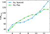 |
Fig. 2. FoM for w0wa as we increase the number of redshift bins generated by assigning galaxies to the equally spaced or equally populated redshift bins. |
Our method of improving the selection of redshift bins takes the equally spaced case as a starting point for the tomography optimisation2. By sampling the space of non-overlapping redshift bin configurations, we attempt to find better configurations with feasible computation times even while employing a realistic pipeline of analysis.
Finding an optimal tomographic configuration for 3 × 2pt analysis requires taking into consideration source and lens galaxies’ mutual dependence. Since the optimal tomographic configuration for the source galaxies depends on the configuration for the lens galaxies and vice versa, both configuration spaces should be sampled simultaneously. In practice, this is much less efficient, as we discuss in Appendix D; thus, an alternative method must be employed. We decided on sampling by alternating between the source and lens bin configurations iteratively. That is, we ran our Fisher pipeline of analysis fixing the tomography of the source galaxies while varying the lens’ tomography or vice versa, sampling 200 randomly perturbed tomographic configurations per iteration. The perturbations to the tomographic configuration consist of a displacement of the edges of each bin in the form of a Gaussian noise with a standard deviation equal to the half-width of the bin, discarding overlapping edges. After running each iteration, the tomographic configuration that yields the highest FoM for a given sample was fixed while perturbed configurations of the other sample were explored, with this being repeated until the FoM converged.
In Fig. 3 we show the performance of this method by optimising the tomography for a fiducial case using eight redshift bins. Our reference is the FoM for equally spaced redshift bins and the improvement in FoM increases over the first few iterations over source and lens tomographic optimisations before rapidly converging, demonstrating the effectiveness of our method in reaching an optimised redshift bin. The computational resources needed to perform a single iteration are 1200 CPU hours for the most expensive case with ten redshift bins.
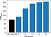 |
Fig. 3. Improvement in the FoM for w0wa as we iteratively optimise the source (Si) and lens (Li) tomography. |
The evolution of the optimised FoM over five iterations is similar for other numbers of redshift bins, coinciding in that, after two iterations sampling the source galaxies binning and two iterations sampling lens galaxies binning, the algorithm has basically converged. Based on this, we implemented our method for different science cases and different numbers of redshift bins limited to four iterations. We also present a brief discussion regarding the numerical stability of the Fisher matrices as computed with CosmoSIS in Appendix E.
4. Results
Having validated the methodology for the optimisation method and determined a convergence criteria based on a set of test cases. We then proceeded to apply it to different numbers of redshift bins (from 3 to 10) and optimised for two different targets: the FoM for w0wa alone, optimising for the improvement of the constraints for the two parameters irrespective of the effect on the constraints on the rest of the parameters of the model, and the FoM for the whole set of cosmological parameters of w0waCDM.
4.1. Tomography optimisation for 3 × 2pt analysis: w0wa
Differentiating evolving DE models from ΛCDM requires a precise measurement of the dynamics of structure formation over very large timescales. For this reason, low-redshift surveys struggle to detect such subtle effects. Stage IV surveys that reach higher redshifts will be able to better characterise the w0 and wa parameters. We show that optimising the tomographic configuration specifically to maximise information about the DE equation of state parameters results in substantial improvements in their constraints.
The first iteration of the optimisation process samples different configurations for the tomography of the source galaxies, while fixing the tomographic configuration of the lens galaxies to the equally spaced case. As we see in the ‘S1’ line in the top panel of Fig. 4, this first sampling of only the source sample does not lead to a major improvement in the FoM. However, with the second iteration of the algorithm, fixing the source sample to the best-performing tomography and sampling the lens configurations, the improvement in our metric increases further. Subsequent iterations may help with the stability of the optimisation by reducing the variance in the FoM of the optimised configuration but do not increase the FoM any further.
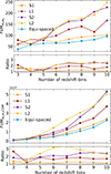 |
Fig. 4. Improvement on information as the tomography is iteratively optimised. The top panel shows the case of FoMw0 wa optimisation for four iterations of the optimisation. The metric in this case quantifies information for just w0 and wa. The bottom panel shows the FoMw0 wa optimisation for four iterations of the optimisation. The metric in this second case quantifies information for the seven cosmological parameters of w0waCDM. |
The resulting FoM after applying our optimisation method is shown in the top panel of Fig. 4, where we see an improvement in our FoM of around two-fold for configurations including a relatively large number of redshift bins (Nbins > 5). A certain degree of variability in the convergence is present, mostly at a lower number of redshift bins. Despite the inherent variation in a stochastic optimisation algorithm, the improvement is consistent across different numbers of iterations and redshift bins. This result illustrates the importance of selecting an optimal tomographic configuration in modern cosmological probes, as the typical case of equally spaced bins is significantly outperformed by our optimal configuration of the source and lens redshift bins. In particular, we find an improvement of ∼25% in the individual constraints for both w0 and wa. Similar results are obtained when simultaneously varying the non-DE model parameters (see the bottom panel of Fig. 4).
As for insights into the physical interpretation of the improvement in the constraints for w0wa, we have to look at the optimised tomographic configurations seen in Fig. 5. In the top left and bottom left panels of Fig. 5, we show the impact of changing the source redshift bins. The optimal configuration converges towards wider redshift bins at high redshift. In contrast, for the lens samples, the optimisation yields thinner lens bins at the low-to-mid redshift range, as is displayed in the top right (L1) and bottom right (L2) panels in Fig. 5. This is understandable: lens bin widths will tend to adjust to the photometric error, σphoto-z, to maximise the signal in clustering measurements (Tanoglidis et al. 2020). In contrast, obtaining a higher signal in WL implies larger bins at high redshift, where fewer galaxies are present, and where the photo-z estimations will be worse but less impactful (Salcedo et al. 2020).
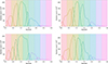 |
Fig. 5. Galaxy number counts for source (left) and lens (right) galaxies for eight redshift bins over several iterations of the optimisation method applied for the dynamical DE model parameters w0wa. The top left panel corresponds to the source sample after the first iteration (S1), the top right panel corresponds to the lens sample after the first iteration (L1), the bottom left panel corresponds to the source sample after the second iteration (S2), and the bottom right to the second iteration of the lens sample (L2). The coloured bands represent the bin edges for the base case of equally spaced bins. |
Since our photo-z catalogue contains very low-redshift galaxies where the WL signal will be lower, the tendency of the algorithm is to disregard those galaxies and put them into a very low-redshift bin with little contribution to the overall constraining power. This is best seen in the bottom left panel in Fig. 5 in the optimisation step involving the second source bin iteration. In the case of the bottom right panel in Fig. 5, corresponding to the second iteration of the lens sample, the low-redshift bin is suppressed by the optimisation algorithm, favouring instead a bigger number density in the mid-range redshift region lens bins. It is also worth noting the tendency to create a wide bin of source galaxies at the redshift mid-range. Given that the lensing signal is larger with lens galaxies halfway (in terms of redshift) to the source galaxies, this suggests that an optimal tomography for 3 × 2pt favours a larger lensing signal at high and mid redshifts, even at the cost of worsening the clustering for wider lens bins. Although these tendencies are hinted at in the top left (S1) and top right (L1) panels of Fig. 5, it is only when further iterations are implemented that this effect is fully realised (see the bottom left (S2) and bottom right (L2) panels in Fig. 5). In fact, the complex interplay between the optimisation of lensing and clustering signals at different redshift ranges is precisely the reason why an efficient numerical tomographic optimisation method needs to be devised.
The initial assessment of four iterations being sufficient to converge into an optimised tomography is compatible with the results for different numbers of redshift bins. Using a larger number of tomographic bins, i.e. ranging from six to ten bins, in the top panel of Fig. 6 we find that there are significant changes with respect to the fiducial tomographic bin configuration; that is, the changes in FoM are larger than the estimated variance of the optimisation. We also find that by the fourth iteration (L2) the gains have stabilised. For this reason we consider the optimisation method to converge after four iterations.
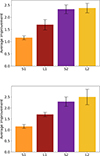 |
Fig. 6. Average improvement and standard deviation from six to ten redshift bins over each iteration of the optimisation method targeting the dynamical DE parameters w0wa (top panel) and targeting the full set of cosmological parameters of w0waCDM (bottom panel). |
4.2. Tomography optimisation for 3 × 2pt analysis: w0waCDM
In the case in which we optimise for the whole set of parameters of our cosmological model – that is, w0, wa, Ωm, Ωb, ns,  , and h – we expect a priori a higher improvement in the FoM for an optimised tomography with respect to the base case of equally spaced bins by virtue of the higher number of parameters. However, by looking at the bottom panel of Fig. 4, the relative gain compared with the optimisation of w0wa is only modestly better hovering at around 2.5-fold. In reality there is an interplay whereby the requirements to constrain certain parameters that are more sensitive to low-redshift growth, such as σ8 (which we sample indirectly through As) or Ωm, and the requirements to constrain those parameters more sensitive to high redshift evolution, such as wa, may differ in terms of optimal tomographic binning.
Given that the number of parameters, and hence the dimensionality of the parameter space, increases, the improvement over iterations as well as the absolute gain in FoM after the method is applied have less variability. This smoother convergence over iterations is expected due to the dependence of the FoM over a larger set of parameters that includes parameters less sensitive than w0 and wa to changes in the tomography. Despite that, we show in the bottom panel of Fig. 6 that the average improvement over a different numbers of redshift bins is similar to the case when we optimise for FoMw0wa. This reiterates the consistency of the algorithm for different target parameters.
4.3. Parameter optimisation dependence
Since our optimisation target, the FoM, depends on which parameters are marginalised, the impact of the optimisation on the parameters that are marginalised over must be assessed. To do that we computed the FoMs with different marginalised parameters than those used during the optimisation. That is, having used the two metrics FoMw0wa and FoMw0waCDM marginalising over all but two or all but seven cosmological parameters, respectively, it could be expected that the optimisation for w0wa could be at the cost of losing constraining power over other cosmological parameters. In order to assess that, we computed the FoMw0waCDM for the Fisher matrices obtained when optimising for FoMw0wa and vice versa. The results shown in Fig. 7 suggest, on the one hand, that using the target of w0wa in our optimisation does not result in a significant decrease in constraining power for the combined set of cosmological parameters. On the other hand, when targeting the whole set of w0waCDM parameters in our optimisation, most of the improvement in constraints must lie in the constraints for w0wa.
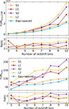 |
Fig. 7. Improvement of off-target cosmological parameter constraints after applying our optimisation method. The top panel shows the values of the FoMw0 waCDM metric for the optimisation targeting w0wa. The bottom panel shows the case computing the FoMw0 wa metric for the optimisation targeting w0waCDM. |
We explored the effect of the optimisation for a given set of parameters (on-target) on the constraints for the rest of the parameters not included in the FoM metric (off-target). In order to do that, we measured the FoM for the on-target and off-target parameters after the optimisation process and we compared the relative improvement with respect to the case with equally spaced binning. In Table 2 we show the relative improvement for the on-target and off-target FoM. The expectation is that the improvement should be highest for the on-target parameters, although the stochastic nature of the method introduces some variation in the relative improvement. For example, performing the optimisation targeting (w0, wa) results in a relative improvement of ΔFoMw0wa = 2.45, larger than the off-target improvement computing the metric for the set of parameters of w0waCDM, with ΔFoMw0waCDM = 2.17. This similar albeit smaller relative improvement of off-target parameters indicates that the optimisation method does not result in worsening the constraints of the off-target parameters of the model. We discuss in more detail the impact of the optimisation on off-target cosmological parameters in Appendix F. We also present the case in which the single probe of WL was used in the analysis instead of 3 × 2pt. In this case, the constraining power is smaller to begin with, resulting in much greater variance and a case in which the off-target improvement of ΔFoMw0waCDM = 4.78 is larger than on-target. From this we conclude that our method performs most consistently when the constraining power is larger.
Comparison of on-target and off-target improvement in our metric after applying our optimisation method.
5. Discussion
The characterisation of DE is one of the most ambitious goals of current physics. A significant amount of resources has been invested for that objective. For example, recent DESI results (Abdul Karim et al. 2025) have hinted at possible deviations from ΛCDM from the combination of measurements of baryon acoustic oscillations, type-Ia supernovae measurements, and cosmic microwave background data. Their results favour w0waCDM with a significance of 2.8 − 4.2σ. While DESI used spectroscopic data to study LSS, other surveys will use a complementary approach, based on photometric data to test dynamical DE models. However, optimising the tomographic sample selection of photometric galaxy surveys for the study of DE is still an open question.
Our work provides a rather general end-to-end cosmological inference pipeline to optimise dark-energy constraints from 3 × 2pt analyses for next-generation galaxy surveys. In particular, we explore configurations beyond the fiducial paradigm of equal-width or equally populated redshift bins in a fast and robust way. In doing so, we show that photometric surveys could benefit from incorporating optimised tomographic selections in their analysis procedure, at least doubling the DE FoM thanks to our optimisation method.
We have implemented our pipeline for a wide range of redshift bin configurations. The reason is two-fold: to show the robustness of the method over many analysis set-ups and to assess the impact of an optimisation as the number of tomographic bins is increased. We have found that our method is indeed robust and our convergence criteria sufficient for six or more redshift bins. The degree of relative improvement of the FoM after the four iterations was similar for six or more redshift bins as well.
We performed our optimisation method using our own stage-IV-like photometric catalogue and with a fairly realistic analysis pipeline, with results consistent with Euclid Collaboration: Blanchard et al. (2020) for the same number of redshift bins. Thus, we expect our improvement to be applicable in future analysis, implying an improvement in the constraints of the individual parameters of w0 and wa of about 25%.
Previous work from Euclid Collaboration: Pocino et al. (2021) compared equally spaced tomographic bins and equally populated bins, finding an optimal configuration for each number of redshift bins. They found that, as the number of redshift bins changes, the optimal case between equally populated and equally spaced bin configurations can change as well, similarly to what we found (see Fig. 2). However, the relative improvement between the two configurations in their case was smaller than with our method. The work of Taylor et al. (2018) also explored the issue of using the best tomographic binning strategy. The authors noted, in their particular case using a larger number of redshift bins (20), that equally populated redshift bins can lead to excessively narrow bins in the region of the n(z) with most galaxies, while equally spaced bins result in a loss of information due to a low number of galaxies at high redshift. While they opted for equally spaced bins as optimal in their set-up, their work again highlights the need to be flexible in the way we approach the issue of choosing our tomographic redshift bins.
In the work by Wong et al. (2026), an exploration of the optimal tomographic configuration of 3 × 2pt analysis for Euclid, an ongoing stage IV survey, was performed. The authors performed their exploration with equally spaced, equally populated, and equal comoving distance redshift bins. They used a realistic set-up using mock realisations of Euclid observations and concluded that the best-performing tomography for 3 × 2pt analysis was equally populated bins, with information saturating in ≥7 − 8 redshift bins. Information saturation in a lower number of redshift bins would be expected with the settings of the first Euclid data release, with a smaller sky coverage of 2600 square degrees. In contrast, our work explores a range of tomographic configurations beyond those three. We explored tomographic binning for the source and lens samples separately and, most importantly, in an iterative manner that allows for a quick convergence. We also ensured that the choice of initial conditions does not have an impact on the convergence, as is discussed in Appendix C. Our results show that we can improve the amount of information on w0 and wa by using the highly customised tomographic bins that we obtained. While our method of defining tomographic configurations to explore is numerical, in Sect. 4.2 we present possible physical insights into the optimal configurations of both the source and lens samples.
The CosmoDC2 simulation was also used in the LSST-DESC 3 × 2pt Tomography Optimization Challenge (Zuntz et al. 2021), in which a variety of tomographic configuration algorithms were compared in terms of their ability to improve the information on w0 and wa using 3 × 2pt analysis. Of the methods presented there, some optimised the assignment of galaxies to fixed tomographic bins and others optimised the configuration of bin edges. We compare our method with the latter. Highlighting the complexity of the problem, the optimised edges for 3 × 2pt failed to yield good results for lensing alone. This points to the need of optimising the tomography for specific science cases. However, the methods that used fixed bins and optimised the classification of galaxies into bins plateaued at a metric value of 120-140, inferior to the best-performing methods that optimised the bin edges and reached up to 167. This result strongly emphasises the need to explore redshift bin selections beyond the usual equally spaced or equally populated choices. In this work we used a different set-up using more photometric bands, different footprints, and a much smaller training set (≈105 galaxies to train our SOM vs. ≈106 in their training), but we obtained a larger relative improvement with our optimised redshift bin selection with respect to the equally spaced tomography.
We emphasise that although the method presented here is a proof of concept, it already yields substantial improvements in the constraints for the cosmological parameters in ΛCDM and dynamical DE cosmologies. Increasing the FoM for w0wa by a factor of 2 or more would be comparable to a substantial increase in the sky coverage of a survey. Even acknowledging that forecasts in the Fisher formalism have potential limitations, the improvement that we can expect from applying our method to real data and a full Markov chain Monte-Carlo analysis should be of interest for any current and future photometric surveys aiming to provide competitive cosmological constraints.
6. Conclusions
We have developed a new method of optimising the way in which the tomographic redshift bins for 3 × 2pt analyses in photometric galaxy surveys are selected. As a proof of concept, we generated a photo-z galaxy catalogue from the CosmoDC2 simulation using a SOM and we selected the training and photo-z galaxy catalogues with similar characteristics to current or planned stage IV surveys. We also used a pipeline of cosmological parameter inference to estimate the contours for a set of cosmological DE-related parameters using the Fisher formalism. We used the FoM metric derived from the marginalised Fisher matrix to assess the constraining power of a given choice of tomographic redshift bins in our analysis, and we optimised the sample selection for both the source and the lens galaxy samples separately and in an iterative manner. We did so using sets of 200 perturbed bin edges per iteration and found that the method consistently converges after four iterations: two of the source sample and two of the lens sample. We selected the w0wa parameters of dynamical DE as our target for optimisation, but we found that the improvement in the constraints of those parameters does not come at the cost of a decreased constraining power for the rest of the parameters of the model. In contrast, there is an additional improvement in other cosmological parameter constraints. Overall, we have found an average improvement for w0 and wa of ≈25% based on the FoM values, although Fisher-derived contours suggest that the improvement is most prominent for wa in particular. Furthermore, we have shown the robustness of our optimisation method against different analysis choices. In conclusion, we propose the sample selection optimisation pipeline presented here as a powerful tool to optimise the scientific return of next-generation photometric galaxy surveys.
Acknowledgments
PF and MA acknowledge support form the Spanish Ministerio de Ciencia, Innovación y Universidades, projects PID2019-11317GB, PID2022-141079NB, PID2022-138896NB; the European Research Executive Agency HORIZON-MSCA-2021-SE-01 Research and Innovation programme under the Marie Skłodowska-Curie grant agreement number 101086388 (LACEGAL) and the programme Unidad de Excelencia María de Maeztu, project CEX2020-001058-M. This work has made use of CosmoHub, developed by PIC (maintained by IFAE and CIEMAT) in collaboration with ICE-CSIC. It received funding from the Spanish government (grant EQC2021-007479-P funded by MCIN/AEI/10.13039/501100011033), the EU NextGeneration/PRTR (PRTR-C17.I1), and the Generalitat de Catalunya. Ayuda PRE2020-094899 de la ayuda financiada por MCIN/AEI/10.13039/501100011033 y por FSE invierte en tu futuro.
References
- Abbott, T. M. C., Aguena, M., Alarcon, A., et al. 2022, Phys. Rev. D, 105, 023520 [CrossRef] [Google Scholar]
- Abdul Karim, M., Aguilar, J., Ahlen, S., et al. 2025, Phys. Rev. D, 112, 083515 [Google Scholar]
- Abolfathi, B., Alonso, D., Armstrong, R., et al. 2021, ApJS, 253, 31 [CrossRef] [Google Scholar]
- Albrecht, A., Bernstein, G., Cahn, R., et al. 2006, arXiv e-prints [arXiv:astro-ph/0609591] [Google Scholar]
- Asgari, M., Lin, C.-A., Joachimi, B., et al. 2021, A&A, 645, A104 [NASA ADS] [CrossRef] [EDP Sciences] [Google Scholar]
- Bhandari, N., Leonard, C. D., Rau, M. M., et al. 2021, arXiv e-prints [arXiv:2101.00298] [Google Scholar]
- Blazek, J., MacCrann, N., & Troxel, M. A. 2019, Phys. Rev. D, 100, 103506 [NASA ADS] [CrossRef] [Google Scholar]
- Carretero, J., Tallada, P., Casals, J., et al. 2017, Proceedings of the European Physical Society Conference on High Energy Physics [Google Scholar]
- Chevallier, M., & Polarski, D. 2001, Int. J. Mod. Phys. D, 10, 213 [Google Scholar]
- Dalal, R., Li, X., Nicola, A., et al. 2023, Phys. Rev. D, 108, 123519 [CrossRef] [Google Scholar]
- Desjacques, V., Jeong, D., & Schmidt, F. 2018, Phys. Rept., 733, 1 [NASA ADS] [CrossRef] [Google Scholar]
- Euclid Collaboration (Blanchard, A., et al.) 2020, A&A, 642, A191 [NASA ADS] [CrossRef] [EDP Sciences] [Google Scholar]
- Euclid Collaboration (Pocino, A., et al.) 2021, A&A, 655, A44 [NASA ADS] [CrossRef] [EDP Sciences] [Google Scholar]
- Euclid Collaboration (Lepori, F., et al.) 2022, A&A, 662, A93 [NASA ADS] [CrossRef] [EDP Sciences] [Google Scholar]
- Euclid Collaboration (Mellier, Y., et al.) 2025, A&A, 697, A1 [Google Scholar]
- Fang, X., Krause, E., Eifler, T., et al. 2020, JCAP, 05, 010 [Google Scholar]
- Heavens, A., Refregier, A., & Heymans, C. 2000, MNRAS, 319, 649 [NASA ADS] [CrossRef] [Google Scholar]
- Heitmann, K., Finkel, H., Pope, A., et al. 2019, ApJ, 245, 16 [Google Scholar]
- Heymans, C., Trüster, T., Asgari, M., et al. 2021, A&A, 646, A140 [NASA ADS] [CrossRef] [EDP Sciences] [Google Scholar]
- Howlett, C., Lewis, A., Hall, A., et al. 2012, JCAP, 04, 027 [Google Scholar]
- Ivezić, Ž., Kahn, S. M., Anthony Tyson, J., et al. 2019, ApJ, 873, 111 [NASA ADS] [CrossRef] [Google Scholar]
- Kitching, T. D., Taylor, P. L., Capak, P., et al. 2019, Phys. Rev. D, 99, 063536 [Google Scholar]
- Korytov, D., Hearin, A., Kovacs, E., et al. 2019, ApJS, 245, 26 [NASA ADS] [CrossRef] [Google Scholar]
- Lewis, A., Challinor, A., & Lasenby, A. 2000, ApJ, 538, 473 [Google Scholar]
- Linder, E. V. 2003, PRL, 90, 091301 [NASA ADS] [CrossRef] [Google Scholar]
- Masters, D., Capak, P., Stern, D., et al. 2015, ApJ, 813, 53 [Google Scholar]
- Moskowitz, I., Gawiser, E., Bault, A., et al. 2023, ApJ, 950, 49 [Google Scholar]
- Porredon, A., Crocce, M., Fosalba, P., et al. 2022, Phys. Rev. D, 106, 103530 [NASA ADS] [CrossRef] [Google Scholar]
- Prince, H., Rogozenski, P., Šarčević, N., & Gawiser, E. 2025, Am. Astron. Soc. Meet. Abstr., 245, 250 [Google Scholar]
- Salcedo, A. N., Wibking, B. D., Weinberg, D. H., et al. 2020, MNRAS, 491, 3061 [Google Scholar]
- Sipp, M., Schäfer, B. M., & Reischke, R. 2021, MNRAS, 501, 683 [Google Scholar]
- Takahashi, R., Sato, M., Nishimichi, T., et al. 2012, ApJ, 761, 152 [Google Scholar]
- Tallada, P., Carretero, J., Casals, J., et al. 2020, Astron. Comput., 32, 100391 [Google Scholar]
- Tanoglidis, D., Chang, C., & Frieman, J. 2020, MNRAS, 491, 3535 [NASA ADS] [CrossRef] [Google Scholar]
- Taylor, P. L., Kitching, T. D., & McEwen, J. D. 2018, Phys. Rev. D, 98, 043532 [Google Scholar]
- Tutusaus, I., Martinelli, M., Cardone, V. F., et al. 2020, A&A, 643, A70 [EDP Sciences] [Google Scholar]
- Wang, Y. 2008, Phys. Rev. D, 77, 123525 [NASA ADS] [CrossRef] [Google Scholar]
- Wong, J. H. W., Brown, M. L., Duncan, C. A. J., et al. 2026, A&A, in press, https://doi.org/10.1051/0004-6361/202553742 [Google Scholar]
- Wright, A. H., Stölzner, B., Asgari, M., et al. 2025, A&A, 703, A158 [NASA ADS] [CrossRef] [EDP Sciences] [Google Scholar]
- Zuntz, J., Paterno, M., Jennings, E., et al. 2015, Astron. Comput., 12, 45 [NASA ADS] [CrossRef] [Google Scholar]
- Zuntz, J., Lanusse, F., Malz, A. I., et al. 2021, OJAp, 4, 13418 [Google Scholar]
We have checked that starting from equally populated z-bins we get consistent results.
But we note that we get consistent results when starting from equally populated bins, as is shown in Appendix C.
Appendix A: SOM implementation
In order to utilise the SOM to estimate photo-z, it must first be trained. The training starts with the initialisation of the SOM, where we define the weights of each voxel. The weights are set to random colour values using a Gaussian distribution centred at the average colour of the training sample galaxies. The training sample would consist of spectroscopic galaxies in a survey. Since we used a simulated catalogue our training sample contains the true redshift of the galaxies. The training of the SOM is carried out in a sequential manner by finding the voxel’s weights that more closely match the training galaxy colours. For each training galaxy, the weights of the whole SOM are modified to more closely reflect the galaxy colour vector, x. To find the best matching voxel to each galaxy we compute the distance between a given voxel’s weights and a given galaxy as:
 (A.1)
(A.1)
where σi is the error in each colour measurement for a given galaxy. The voxel jk whose distance djk corresponds to the smallest value becomes the best-matching unit (BMU) for that particular galaxy. The weights of all the voxels in the map are updated. The amount of change is related to the distance from each voxel to the BMU for a given iteration, with closer voxels changing more. For each iteration in the training, the weights of each voxel in the map change in the following way:
 (A.2)
(A.2)
where j′k′ are the indices of the BMU voxel, t is the number of iterations of learning that have been carried out. Our choice was to have four iterations per galaxy in the training sample, as there was little to no improvement after training with a single iteration per galaxy already.
The weights of the map are all changed in each iteration with the goal of forming clusters based on the colour phenotype of galaxies. With a(t) being a learning function that decreases the impact of each learning iteration as the number of iterations, Niter, used in learning increases and a proximity parameter, Hj′k′,jk(t), that modulates the degree of change in the voxels surrounding the BMU for each iteration:
 (A.3)
(A.3)
 (A.4)
(A.4)
with Dj′k′,jk being the distance between the position of the BMU at j′k′ and the voxel jk on the map and σ(t) modulating the diminishing effects of each iteration as a function of the distance between voxels on the map as:
 (A.5)
(A.5)
with n1 being the shortest side of the map. The learning process of the SOM is such that the initial learning iterations will have a greater impact on the weights and also have such impact over a larger area of the map around the BMUs. As the training progresses and the iteration parameter t increases, each new iteration will have a smaller impact on the weights and the impact will be limited to the BMU and a few voxels around it. In this way, colour phenotype clusters are first defined in the initial stages of the training and, as the iterations continue, the clusters become more differentiated with specific colour phenotypes.
The degree of completeness of the training sample will determine the regions in colour phenotype that will be covered by the SOM. This means that galaxies at high redshift, being less common, will be poorly characterised compared to those at lower redshift. Each voxel will have a redshift distribution composed of the true redshift of the galaxies assigned to that voxel during the training of the SOM. In order to reduce the number of catastrophic outliers, voxels with less than three redshifts in their n(z)’s are not used for the photo-z estimation. We perform our learning process with Niter = 4 × 10⁵ iterations, which is 4 times the training sample size, although using as many iterations as galaxies in the sample is enough according to Kitching et al. (2019). Galaxies in the training sample will be cycled through in random order.
The size of the SOM in terms of its number of voxels is also relevant to the performance of the SOM. It must be large enough so that phenotype clusters can be formed but small enough to not be sparsely populated with many clusters. The former problem would lead to a poor characterisation of galaxies and the latter would be analogous to over-fitting. In addition, the shape of the SOM will also affect the formation of phenotype clusters. Rectangular shapes allow for more differentiated phenotype clusters to be formed during the training process. Our choice was to use a rectangular SOM of size 100 by 140 voxels, similar to the one in Kitching et al. (2019), which is 75 by 150.
In the top panel of Fig. A.1 we can see the resulting SOM. The redshift value of each voxel is determined during training by the average redshift of galaxies from the training sample that were assigned to that voxel. We show the resulting redshift map of the SOM, where redshift clusters appear. While some areas have smooth gradients in redshift, there are abrupt differences that account for similar colour phenotypes with substantially different redshift. This showcases the capacity of the SOM to distinguish colour phenotypes in order to avoid redshift degeneracies.
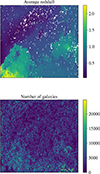 |
Fig. A.1. SOM visualisations. The top panel shows the redshift map of the SOM. The average redshift of the galaxies from the training sample is assigned to each voxel in the map. White voxels had no galaxies assigned during training. The bottom panel shows the galaxy density map of the SOM. The number of photo-z galaxies that are assigned to each voxel. |
To generate the photo-z assigned to each galaxy, a sample is generated from a normal distribution defined with the mean and standard deviation of the galaxies’ redshift in each voxel. We have found this method preferable to directly using the voxel’s n(z) distribution as a probability distribution when estimating photo-z to reduce over-fitting. The resulting distribution of photo-z galaxies on the SOM can be seen in the bottom panel of Fig. A.1. The most populated areas of the SOM coincide with areas of medium redshift while high-redshift areas are less populated. Galaxies with similar colour phenotypes will be close on the map; having clusters of high and low redshift close on the map indicates the capacity of the SOM to differentiate galaxies at low and high redshift despite similar colour profiles.
Appendix B: Additional priors
In a realistic analysis, the galaxy distribution and the shear measurement can be calibrated. Hence we can consider an informative prior on the corresponding nuisance parameters for these quantities. This is even more important as the number of tomographic bins increases, since the higher number of parameters reduces the constraining power. In this analysis we consider DES Y3-based n(z) and shear calibration priors. While we have not used priors derived from stage IV forecasts, we do expect a significant improvement in these calibrations when moving from stage III to stage IV data. Therefore, the stage III priors considered in this analysis can be seen as a conservative choice. We also note that we only consider the width of the prior on the nuisance parameters. We center all priors on nuisance parameters at their fiducial values.
In practice, since the tomographic redshifts in the DES analysis have been chosen by different criteria to ours and up to a lower redshift depth, we have opted to use priors with a width given by the average of the DES’ priors widths. This means that we applied Gaussian priors where the standard deviation is the same for all tomographic bins and given by the average value of the 4 DES bins. The exact values of the standard deviations we considered are: σstd, lensΔzi = 0.0075, σstd, sourceΔzi = 0.015, σstd, lensσi = 0.0623, and σstd,mi = 0.0083. The inclusion of these Gaussian priors has been performed in the Fisher formalism by adding the corresponding matrix to the Fisher matrix. This implies generating a matrix that is empty except for the diagonal terms that correspond to each of the priors, which instead have the values  , and adding said matrix to the corresponding Fisher matrix.
Appendix C: Optimisation with equally populated bins as initial point
For the sake of completeness, we have also run the optimisation algorithm with another set of initial conditions. Choosing equally populated redshift bins instead of equal-width bins does not change the outcome of the optimisation. Looking at Fig. C.1 we can see how after applying the iterative optimisation process in three instances we already recover an improvement in the FoM for w0wa of a factor above two. This is expected because the method has the freedom to explore tomographic configurations well beyond the initial conditions.
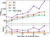 |
Fig. C.1. Optimisation starting from equally populated redshift bins. |
Appendix D: Simultaneous optimisation of source and lens samples
We see in Fig. D.1 the results of using a simpler approach where we compute the FoM varying the n(z) of both the source and lens tomography simultaneously. Using this method instead of varying the n(z) of sources for a fixed lens configuration and vice versa is much less efficient in reaching an optimised tomography. This is because the optimal n(z) of the source galaxies depends on the lens tomography, hence our iterative method can better optimise the samples taking this interplay between lens and source galaxies into account. Thus, the sampling needs to be much larger to converge into an optimal tomography for the source and lens galaxies. The result is that the improvement in the FoM is not as smooth or predictable when we increase the sampled configurations by the same amount as what would correspond to S1, L1, and L2 in the iterative optimisation method. This showcases the advantage of using the iterative method of alternating between source and lens optimisation with respect to sampling both the source and lens tomographic configurations simultaneously.
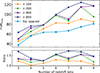 |
Fig. D.1. Simultaneous optimisation of the source and lens samples. Each line corresponds to the FoM of the best-performing tomography when randomly sampling both the source and lens tomographic configurations. The parameter ’n’ corresponds to the total number of runs, with n = 800 being the same number of runs needed for the 4 iterations of the iterative optimisation. |
Appendix E: Numerical stability of the Fisher derivatives
The derivatives that are used in the calculation of the Fisher matrices are performed numerically within the CosmoSIS framework. Certain numerical methods to compute these derivatives have been shown to be susceptible to instabilities (Bhandari et al. 2021). The default method used by the Fisher sampler in CosmoSIS is the stencil method, which involves the calculation of the plain differences at some step sizes and is the fastest method. Another more robust method is included in the sampler, the smooth method, which fits a local polynomial across multiple perturbations and differentiates the smoothed curve. The latter method is less susceptible to instabilities but is more costly computationally. While these numerical instabilities may appear when using the faster stencil method and may result in some variation in the FoM that are computed, the optimisation method is expected to still perform correctly regardless of the chosen numerical method. In order to assess the impact that the use of different methods could have on the pipeline, the following test has been performed.
We have considered the case of six tomographic bins with the optimisation of the w0 and wa parameters. This case has been chosen because it has been shown to converge after the four iterations and is rapidly generated due to the smaller number of parameters in the sampling. The test has been carried out by computing the Fisher matrices with the smooth method instead of the stencil method. We have performed five runs of the optimisation pipeline and computed the mean of the five realisations of the best FoM value each iteration as well as the corresponding standard deviation. For validation, we have also run five realisations of the optimisation method using the stencil method when computing the Fisher matrices and computed the average best FoM and standard deviation as well. The results of this test can be seen in E.1, where the smooth method results in a similar convergence to the stencil case despite a slightly different absolute value of the FoM, which is well within the uncertainties associated with different realisations of the pipeline. From this figure we observe that the convergence over 4 iterations is robust and so is the fact that this optimisation method improves the parameter constraints. Therefore we conclude that the robustness of the method is not affected by the aforementioned numerical instabilities. We note that we keep the stencil method for the numerical derivatives as our baseline as it is significantly faster.
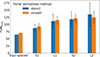 |
Fig. E.1. Comparison of the performance of the optimisation method using the smooth method or the stencil method to compute the derivatives of the Fisher matrix. Showing the average best FoM of each iteration over 5 realisations of the optimisation method for 6 tomographic bins along with the associated standard deviation. |
Appendix F: Optimised likelihood contours
In Fig. F.1 we show the constraints for the w0waCDM model parameters in the base case (equally spaced tomography) and the optimised sample selection case for 8 tomographic redshift bins. Our optimisation method has affected the constraints for wa most dramatically while providing more modest improvements for other cosmological parameters like w0 or As, while other parameters are mostly unaffected. Crucially, our tomographic optimisation does not degrade the constraints for other parameters of the model even when the target was FoMw0wa.
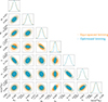 |
Fig. F.1. Likelihood contours at 1-σ and 2-σ estimated through the Fisher matrix for the 7 cosmological parameters of the w0waCDM model. Plotted are the contours obtained with the optimised tomography for w0wa (blue) and with the equally spaced tomography (orange) for 8 redshift bins. |
All Tables
Fiducial values for the systematic effects in our IA modelling, shear calibration, and n(z) errors.
Comparison of on-target and off-target improvement in our metric after applying our optimisation method.
All Figures
|
Fig. 1. SOM performance evaluation. The top panel shows the normalised distributions of the true redshift of galaxies from the simulated catalogue (blue), of the estimated photo-z generated with the SOM (orange), and of the sample used to train the SOM (green). The bottom panel shows the performance of the SOM in the estimation of the photo-z of galaxies. |
| In the text | |
|
Fig. 2. FoM for w0wa as we increase the number of redshift bins generated by assigning galaxies to the equally spaced or equally populated redshift bins. |
| In the text | |
|
Fig. 3. Improvement in the FoM for w0wa as we iteratively optimise the source (Si) and lens (Li) tomography. |
| In the text | |
|
Fig. 4. Improvement on information as the tomography is iteratively optimised. The top panel shows the case of FoMw0 wa optimisation for four iterations of the optimisation. The metric in this case quantifies information for just w0 and wa. The bottom panel shows the FoMw0 wa optimisation for four iterations of the optimisation. The metric in this second case quantifies information for the seven cosmological parameters of w0waCDM. |
| In the text | |
|
Fig. 5. Galaxy number counts for source (left) and lens (right) galaxies for eight redshift bins over several iterations of the optimisation method applied for the dynamical DE model parameters w0wa. The top left panel corresponds to the source sample after the first iteration (S1), the top right panel corresponds to the lens sample after the first iteration (L1), the bottom left panel corresponds to the source sample after the second iteration (S2), and the bottom right to the second iteration of the lens sample (L2). The coloured bands represent the bin edges for the base case of equally spaced bins. |
| In the text | |
|
Fig. 6. Average improvement and standard deviation from six to ten redshift bins over each iteration of the optimisation method targeting the dynamical DE parameters w0wa (top panel) and targeting the full set of cosmological parameters of w0waCDM (bottom panel). |
| In the text | |
|
Fig. 7. Improvement of off-target cosmological parameter constraints after applying our optimisation method. The top panel shows the values of the FoMw0 waCDM metric for the optimisation targeting w0wa. The bottom panel shows the case computing the FoMw0 wa metric for the optimisation targeting w0waCDM. |
| In the text | |
|
Fig. A.1. SOM visualisations. The top panel shows the redshift map of the SOM. The average redshift of the galaxies from the training sample is assigned to each voxel in the map. White voxels had no galaxies assigned during training. The bottom panel shows the galaxy density map of the SOM. The number of photo-z galaxies that are assigned to each voxel. |
| In the text | |
|
Fig. C.1. Optimisation starting from equally populated redshift bins. |
| In the text | |
|
Fig. D.1. Simultaneous optimisation of the source and lens samples. Each line corresponds to the FoM of the best-performing tomography when randomly sampling both the source and lens tomographic configurations. The parameter ’n’ corresponds to the total number of runs, with n = 800 being the same number of runs needed for the 4 iterations of the iterative optimisation. |
| In the text | |
|
Fig. E.1. Comparison of the performance of the optimisation method using the smooth method or the stencil method to compute the derivatives of the Fisher matrix. Showing the average best FoM of each iteration over 5 realisations of the optimisation method for 6 tomographic bins along with the associated standard deviation. |
| In the text | |
|
Fig. F.1. Likelihood contours at 1-σ and 2-σ estimated through the Fisher matrix for the 7 cosmological parameters of the w0waCDM model. Plotted are the contours obtained with the optimised tomography for w0wa (blue) and with the equally spaced tomography (orange) for 8 redshift bins. |
| In the text | |
Current usage metrics show cumulative count of Article Views (full-text article views including HTML views, PDF and ePub downloads, according to the available data) and Abstracts Views on Vision4Press platform.
Data correspond to usage on the plateform after 2015. The current usage metrics is available 48-96 hours after online publication and is updated daily on week days.
Initial download of the metrics may take a while.