| Issue |
A&A
Volume 708, April 2026
|
|
|---|---|---|
| Article Number | A213 | |
| Number of page(s) | 14 | |
| Section | Stellar structure and evolution | |
| DOI | https://doi.org/10.1051/0004-6361/202556766 | |
| Published online | 08 April 2026 | |
Radio timing constraints on the orbital orientation and component masses of PSR J1455−3330
1
Max-Planck-Institut für Radioastronomie, Auf dem Hügel 69, D-53121 Bonn, Germany
2
Jodrell Bank Centre for Astrophysics, University of Manchester, M13 9PL, Cheshire, UK
3
LPC2E, OSUC, Univ Orleans, CNRS, CNES, Observatoire de Paris, F-45071 Orleans, France
4
ORN, Observatoire de Paris, Université PSL, Univ Orléans, CNRS, 18330 Nançay, France
5
Centre for Astrophysics and Supercomputing, Swinburne University of Technology, Hawthorn, VIC 3122, Australia
6
The Australian Research Council Centre of Excellence for Gravitational Wave Discovery (OzGrav), Hawthorn, Australia
7
INAF – Osservatorio Astronomico di Cagliari, Via della Scienza 5, I-09047 Selargius (CA), Italy
8
High Energy Physics, Cosmology & Astrophysics Theory (HEPCAT) Group, Department of Mathematics and Applied Mathematics, University of Cape Town, Rondebosch 7701, South Africa
9
FORTH Institute of Astrophysics, N. Plastira 100, 70013 Heraklion, Greece
10
State Key Laboratory of Radio Astronomy and Technology, Shanghai Astronomical Observatory, CAS, 80 Nandan Road, Shanghai 200030, P. R. China
11
Dipartimento di Fisica “G. Occhialini”, Università degli Studi di Milano-Bicocca, Piazza della Scienza 3, I-20126 Milano, Italy
12
INFN, Sezione di Milano-Bicocca, Piazza della Scienza 3, 20126 Milano, Italy
★ Corresponding author: This email address is being protected from spambots. You need JavaScript enabled to view it.
Received:
6
August
2025
Accepted:
12
January
2026
Abstract
PSR J1455−3330 is a ∼7.98 ms pulsar in a ∼76.17 day nearly circular orbit with a white dwarf companion. In this work, we combine the available Lovell, Nançay decimetric Radio Telescope, Green Bank, and MeerKAT pulsar timing data spanning approximately 30 years to measure the kinematic and relativistic effects of PSR J1455−3330 to constrain its 3D orbital geometry and component masses. We detect a relativistic Shapiro delay signal. We measure a significant orthometric amplitude of h3 = 0.307+0.022−0.026 μs and an orthometric ratio of ς = 0.551+0.057−0.054. We measured the change in projected semi-major axis, x˙ = −202.1+2.5−2.7 × 10⁻¹⁶ s s−1, with high significance, parallax, ϖ = 1.11(6) mas, parallax derived distance 0.90(5) kpc, and a precise total proper motion magnitude of 12.432(2) mas yr−1. A self-consistent analysis of all kinematic and relativistic effects, assuming general relativity, yielded two solutions: (1) a pulsar mass of Mp = 1.39+0.38−0.18 M⊙, a companion mass of Mc = 0.293+0.056−0.026 M⊙, an orbital inclination of i = 63(2)°, and a longitude of the ascending node of Ω = 212(12)° or (2) a pulsar mass of Mp = 1.53+1.10−0.22 M⊙, a companion mass of Mc = 0.309+0.163−0.026 M⊙, an orbital inclination of i = 123(4)°, and a longitude of the ascending node of Ω = 334(12)°. All uncertainties represent the 68.27% credibility region. These results strongly favour a helium-dominated white dwarf companion.
Key words: binaries: general / stars: evolution / stars: neutron / pulsars: general / white dwarfs / pulsars: individual: PSR J1455-3330
© The Authors 2026
 Open Access article, published by EDP Sciences, under the terms of the Creative Commons Attribution License (https://creativecommons.org/licenses/by/4.0), which permits unrestricted use, distribution, and reproduction in any medium, provided the original work is properly cited.
This article is published in open access under the Subscribe to Open model.
Open access funding provided by Max Planck Society.
1. Introduction
Rotating neutron stars that emit beams of electromagnetic radiation from their magnetic poles (i.e. pulsars) are observed as a steady periodic sequence of pulses as the beam sweeps through the observer’s line of sight. This lighthouse-like rotation of a pulsar can be tracked with high precision using pulsar timing and can offer a wealth of information in the field of fundamental physics.
Precise mass measurements of neutron stars are important for studies regarding equations of state (EoS), ultra stripped supernovae explosions, and binary evolution theories. The current observable mass distribution ranges from ∼1.174(4) M⊙ (Martinez et al. 2015, PSR J0453+1559c) to ∼2.08(7) M⊙ (Fonseca et al. 2021, PSR J0740+6620). The highest masses can be used to study EoS, the lowest masses can be used to study ultra-stripped supernovae explosions (Martinez et al. 2015), and everything in between is valuable for studies of binary evolution.
Millisecond pulsars (MSPs) are ‘recycled’ neutron stars that have extremely stable spin periods (P ≲ 100 ms and spin-down Ṗ ≲ 10−17 s s−1) whose pulse times of arrival (ToAs) can be measured with great precision. Around 80% of MSPs are found in binary systems, with companions of varying mass, including main sequence stars, neutron stars, or white dwarfs.
MSPs with helium white dwarf (HeWD) companions, in particular, form after Gyrs of accreting matter onto the neutron star from a low-mass star (Tauris & van den Heuvel 2023). During this stage, the system is visible at X-ray wavelengths as a low-mass X-ray binary. The eccentricities of these binaries are well explained by the orbital period–eccentricity relation (Phinney 1992), where most binary millisecond pulsars have very low orbital eccentricities. The tidal interaction with the red-giant companion circularises the orbits. After Roche-lobe overflow, the pulsar is spun up to millisecond periods, and the companion is left as a HeWD (Radhakrishnan & Srinivasan 1982; Alpar et al. 1982; Tauris & van den Heuvel 2023). In such systems, the binary orbital period, Pb, and mass of the HeWD, MWD, are correlated following the Tauris & Savonije (1999) relation.
In this work, we discuss our timing analysis of the MSP system PSR J1455−3330 (hereafter J1455−3330) using data from the Lovell Telescope, Nançay decimetric Radio Telescope (NRT), Green Bank Telescope (GBT), and MeerKAT telescope. J1455−3330 was discovered in a Southern Hemisphere survey search for millisecond pulsars along the Galactic disk using the 64-m CSIRO Parkes Murriyang radio telescope (Lorimer et al. 1995). The short spin period (P ∼ 7.98 ms), and small spin-down rate (Ṗ ∼ 2.43 × 10⁻²⁰ s s−1) indicate that the pulsar is recycled. The small mass function (f = 0.00627 M⊙), under the assumption that the pulsar has a canonical mass of 1.4 M⊙ (Lorimer et al. 1995), results in a minimum companion mass of Mc = 0.27 M⊙. This minimum companion mass and the nearly circular orbit (e∼ 0.00016) indicate that the companion is a white dwarf.
The EPTA Collaboration (2023) detected a highly significant (33σ, where 1σ is the 68.27% credibility level) change in its projected semi-major axis (ẋ) and a moderate (2 σ) Ṗb value using the available Lovell and Nançay data. The detection of ẋ provides us with an opportunity to constrain the 3D orbital geometry of the system as in PSR J1933−6211 (Geyer et al. 2023), PSR J2222−0137 (Guo et al. 2021), and PSR J0955−6150 (Serylak et al. 2022).
The stable timing properties, previously detected PK parameters, and close proximity (DM = 13.56 cm−3 pc) make J1455−3330 a favourable system for component mass measurements. J1455−3330 was observed with MeerKAT from April 2019 to April 2024 under the MeerTime Large Survey Project (Bailes et al. 2020) as part of two sub-projects: the relativistic binary timing programme (Relbin; Kramer et al. 2021) and the pulsar timing array programme (MPTA; Spiewak et al. 2022). The main objectives of Relbin are to observe compact relativistic binary pulsar systems to measure potential relativistic effects, test theories of gravity, and measure NS masses. The PTA programme aims to search for low-frequency gravitational waves by regularly observing and timing many stable millisecond pulsars.
In this paper, we aim to place constraints on the component masses by using the available Lovell, Nançay, Green Bank, and recently acquired MeerKAT data. We used the measured proper motion, change in the projected semi-major axis, and the Shapiro delay signal detected for the first time to constrain the system’s component masses and orbital orientation.
The structure of this paper is as follows. In Sect. 2 we discuss the observations and the preliminary data analysis to obtain the required times of arrivals. In Sect. 3, we describe the polarisation profile of the pulsar and the fit of its linear polarisation using the Rotating Vector Model (RVM; Radhakrishnan & Cooke 1969). In Sect. 4 we describe the timing analyses, orbital model selection, and noise model selection. The timing results, measured post-keplerian parameters, component mass estimations, and orbital orientation constraints are presented in Sect. 5. In Sect. 6, we discuss the implications of the results, infer the formation and evolution of the system, and discuss the future prospects.
2. Observations, data acquisition, and reduction
In this work, we use data from four different telescopes: the 76-m Lovell Telescope in the United Kingdom, the 94-m equivalent NRT in France, the 100-m GBT in the United States, and the MeerKAT 64-dish array in South Africa. All radio observations and data reduction are detailed below and listed in Table 1.
Observing systems and timing datasets of J1455−3330.
2.1. Lovell Telescope
J1455−3330 was typically observed for 30 minutes per session, once every 10 days with a subintegration time of 10 s (Hobbs et al. 2004). The data used in this work were recorded between October 1992 and June 2024 with an analogue filterbank (AFB) until January 2009 and the digital filterbank (DFB) thereafter. The data recorded with the AFB have a central frequency of 1402 MHz and an observing bandwidth of 64 MHz. The DFB is a clone of the Parkes Digital FilterBank, with a central observing frequency of 1400 MHz, and a bandwidth of 128 MHz split into 512 channels. From September 2009, the centre frequency was changed to 1520 MHz, and the bandwidth increased to 512 MHz (split into 1024 channels), of which ∼380 MHz was usable, depending on RFI conditions. There are no standard polarisation calibrations applied to the DFB data, but the power levels of both polarisations are manually and regularly adjusted via a set of attenuators. An on-site H-maser clock was used to estimate local time, which has been corrected to UTC using recorded offsets between the maser and GPS satellites (Desvignes et al. 2016).
The data were first incoherently dedispersed to the DM of the pulsar and folded at the best-known period. These folded profiles were cleaned using the PSRCHIVE paz and pazi tools, and the ToAs were generated by cross-correlating an analytic noise-free template with the time-integrated, frequency-scrunched, total intensity profile. The template was generated using the paas tool to fit a set of von Mises functions to a profile created using psradd on the high signal-to-noise (S/N) ratio observations.
2.2. Nançay decimetric Radio Telescope
We selected NRT observations carried out with the Berkeley-Orléans-Nançay (BON) backend from January 2005 until August 2011, and with the NUPPI backend (a version of the Green Bank Ultimate Processing Instrument, installed at the NRT) after it became the primary pulsar timing instrument in August 2011, until June 2023. BON observations were carried out at 1.4 GHz, over a bandwidth of 64 MHz until mid-2008, and then over 128 MHz. NUPPI observations were done at a central frequency of 1.484 GHz, and over a larger bandwidth of 512 MHz. BON and NUPPI observations were coherently dedispersed, and were typically ∼1 h long.
Daily observations were fully scrunched in time. BON observations were scrunched in frequency in order to form two frequency sub-bands of 32 MHz (resp. 64 MHz) for the data taken before (resp. after) mid-2008. NUPPI data were split into four sub-bands of 128 MHz each. High S/N template profiles for the BON and NUPPI datasets were created by summing the eight observations with the highest S/N, and smoothing the results. ToAs were finally extracted from each observation using the Matrix Template Matching (van Straten 2006) implemented in the pat routine of PSRCHIVE. Additional information about the NRT and about the preparation of NRT pulsar timing data can be found in Guillemot et al. (2023).
2.3. Green Bank Telescope
Observations were taken at 1.4 GHz using the Rcvr_1_2 receiver and 800 MHz using the Rcvr_800 receiver with two different backends (GASP and GUPPI). At 1.4 GHz, we used the data recorded with the GASP backend, with bandwidth ∼64 MHz from August 2004 until February 2010. Similarly, at 1518 MHz, we used the data recorded with the GUPPI backend with a bandwidth of 640 MHz from August 2010 until March 2020.
At 800 MHz we used the GASP backend observations (at central frequency 844 MHz, with bandwidth ∼64 MHz) from July 2004 until January 2011 and the GUPPI backend observations (at central frequency 820.5 MHz, with bandwidth ∼180 MHz) from March 2010 until April 2020.
We used the narrowband generated ToAs published in the North American Nanohertz Observatory for Gravitational Waves (NANOGrav) 15 yr dataset (Agazie et al. 2023) where a separate ToA is measured for each frequency channel. The ToA creation follows a standard approach which uses up to 30-minute time-averaged cleaned and calibrated profiles. All profiles for a given receiver band are aligned, weighted by its S/N ratio, and summed to create a final integrated pulse profile. Its average profile is then ‘denoised’ using wavelet decomposition and thresholding to create a final standard template. All narrowband ToAs, were then generated using the Fourier-domain algorithm as implemented in the PSRCHIVE program pat. This method determined each ToA and its uncertainty via a least-squares fit for the pulse phase shift between an observed total-intensity pulse profile and the aforementioned standard template profile.
2.4. MeerKAT telescope
Observations under the PTA programme were obtained using the MeerKAT telescope between April 16 2019, and April 11 2024. These observations were ∼480 s each and were regularly spaced, with a mean cadence of two weeks. The RelBin observations were longer and were aimed at obtaining good orbital coverage. In particular, the RelBin dataset contains multiple 2 h observations and one 4 h (MJD 60302.15) observation taken close to and across superior conjunction to improve the significance of a Shapiro delay measurement.
The MeerKAT observations were recorded using the L-band receiver (856–1712 MHz) with the 1K (1024) channelisation mode, using the Pulsar Timing User Supplied Equipment (PTUSE) backend (Bailes et al. 2020). The PTUSE outputs coherently dedispersed folded pulsar archives with 1024 phase bins across the pulse period of 7.98 ms.
Standard array calibration was applied before the observations using the MeerKAT science data processing pipeline (SDP). Details of which can be found in Serylak et al. (2021). Before April 9th, 2020, offline polarisation calibration was implemented using the steps outlined in Serylak et al. (2021). After April 9, 2020, online polarisation calibration was carried out where the Tied Array Beam data stream input to PTUSE produces polarisation calibrated L-band pulsar data products.
All MeerTime observations were reduced using the MEERPIPE pipeline1, which produces cleaned archive files using a modified version of coastguard (Lazarus et al. 2016) with varying decimation (using standard PSRchive/pam commands). The archives used in this analysis uses the output products with 1024 frequency channels across the inner 775.75 MHz of MeerKAT L-band, 59 sub-integrations and full Stokes information. To increase the S/N per ToA, we reduced the channelisation to eight frequency channels for all archives and all longer-duration observations were decimated to have a minimum integration length of 3600 s.
Before template creation, all visible residual RFI were removed manually using pazi. All observations were then added in time using PSRadd/PSRCHIVE. A MeerKAT multi-frequency template was created by decimating the added data to a single subintegration, eight frequency channels, and four Stokes polarisations using the pam/PSRCHIVE command. Analytic frequency-resolved standards were created from this high S/N template by applying wavelet smoothing using PSRmooth/PSRCHIVE. This analytic template was subsequently used to apply matrix template matching (van Straten 2004, 2013) creation using pat/PSRCHIVE on the individual MeerKAT data products described in Sect. 2.4.
Lastly, we manually removed individual ToAs with uncertainties larger than 52 times the RMS (∼3.2 μs) from all datasets (after visual inspection that confirmed that the large ToA uncertainties were due to low S/N detections). The time-integrated, frequency-resolved standard profiles from the MeerKAT data are shown in Fig. 2.
3. Pulsar geometry
Throughout this paper, we use the ‘observer’s convention’ to quote angles and vectors, unless otherwise stated. These angles are defined in Fig. 1, where the position angle (PA; Ψ) and the longitude of the ascending node (Ω) increase counter-clockwise on the plane of the sky (starting from north) and the orbital inclination, i, is defined as the angle between the orbital angular momentum and the vector from the pulsar to the Earth.
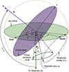 |
Fig. 1. Definition of angles and conventions used in this paper. Throughout this paper, we adopt the ‘observer’s convention’ for all geometric quantities. The fundamental reference plane is in green, and the orbital plane is in purple, with the corresponding unit vectors coloured the same way. S denotes the spin angular momentum, which is aligned with the orbital angular momentum. The magnetic axis (μ) is misaligned from S by the misalignment angle α. The pulsar emission cone has an opening angle ρ, and is cut through by our line of sight at an impact angle β. ζ = α + β is the latitude of the spin axis, which is the same as the orbital inclination angle (i) for spin-aligned systems. |
The emitted electromagnetic waves from a pulsar are polarised along the magnetic field lines, which point radially outwards along the pulsar’s emission cone. As the pulsar’s beam moves across the line of sight, the observer sees these magnetic field lines under an ever-changing angle. This effect can be viewed as a variation in the PA of the linear polarisation of the pulse profile across the pulsar longitude. Under ideal assumptions where the magnetic field is assumed to be dipolar and the plane of linear polarisation rotates rigidly with the pulsar, the PA variation results in an S-shaped swing.
We can infer the geometry of J1455−3330 from the highly resolved swing of the polarisation angle across the main pulse using the Rotating Vector Model (RVM; Radhakrishnan & Cooke 1969). The RVM describes Ψ as a function of the pulse phase, ϕ, depending on the magnetic inclination angle, α, and the viewing angle, ζ′, which is the angle between the line-of-sight vector and the pulsar spin and can be described as,
 (1)
(1)
Note that all angles are expressed in RVM/DT92 convention; therefore, ζ and i in the observer’s convention are related to ζ′ by i ∼ ζ = 180 − ζ′.
The RVM does not always describe the polarisation properties of a pulsar (particularly MSPs) well. However, in cases where the RVM does apply, it can be a valuable tool for breaking the sense of the inclination angle obtained from Shapiro delay measurements, enabling a more precise determination of the 3D orbital orientation.
The top panel of Fig. 2 shows the polarisation profile of J1455−3330 as recorded with the MeerKAT L-band receiver and corrected for the rotation measure given in Spiewak et al. (2022), the middle panel of Fig. 2 shows the evolution of the PA across the pulsar’s phase, and the bottom panel shows the resulting residuals. The PAs are measured in the observer’s convention and exhibit sudden jumps at the edges of the main pulse (MP), coincident with sharp drops in the total linear polarisation. These characteristics can be explained by orthogonal polarisation modes (OPMs; Manchester 1975) and are thought to arise from the propagation effects in the pulsar magnetosphere, or may be intrinsic to the pulsar’s emission (Gangadhara 1997).
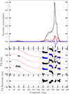 |
Fig. 2. Polarisation profile of J1455−3330 obtained from integrating 32.2 hours of observations with the MeerKAT L-band receiver. The black, red, and blue lines in the top panel indicate the total intensity, linear polarisation fraction, and circular polarisation fraction, respectively. The middle panel shows the evolution of the PA across the pulsar’s phase. The PA exhibits the characteristic swing as well as some phase jumps. The red solid line corresponds to the RVM fit to the PA, and the dashed line shows the RVM solution separated by 90° from the main fit to include the jumped PA values (blue dots). The bottom panel shows the PA residuals. |
We determine the RVM parameter posteriors in their joint parameter space following the method outlined in Johnston & Kramer (2019) using the polarisation angle measurements obtained from all black and blue data points in the middle panel of Fig. 2 (from the MeerKAT observations). The model accounts for the possibility of orthogonal polarisation mode jumps and includes the corrected values in the fit. Points that deviate from the RVM-like swing, shown as grey points, are removed. The red solid line corresponds to the RVM fit to the PA, and the dashed line shows the RVM solution separated by 90° from the main fit to include the jumped PA values (blue dots).
We performed six different fits (which are summarised in Table 2) with varying priors on ζ′: (1) ζ′< 90°; (2) ζ′> 90°, (3) 53° < ζ′< 70° and (4) 110° < ζ′< 127°. The priors of Runs 3 and 4 reflect the constraints on ζ imposed from (both senses) of the inclination angle measured from timing (See Section 5.9). A fifth and six fit reflect recent considerations presented by Kramer & Johnston (2025), who proposed that the weak pulse component preceding the main pulse by about 150 deg (see Fig. 2) is not originating from the polar cap but from beyond the light cylinder. In this case, its corresponding PA values should be ignored by a fit of the RVM.
α and ζ′ priors and posteriors, log likelihood, and implied inclination angle, i, for six different RVM model fits.
An unconstrained fit to the entire profile shows that Run 2 is the best-fit model, implying an orbital inclination angle of approximately 67°. This can be compared to the timing results discussed later (see Sect. 5.9), as the viewing angle is consistent with the range implied by the sine of the orbital inclination angle (sin i). Constraining the fit of the parameter zeta to a similar range yields the same result for Run 4. In contrast, Run 3’s solution attempts to converge with that of Run 1. We also tested solutions following the arguments by Kramer & Johnston by ignoring the weak component in Runs 5 & 6. Run 6 yields a very similar result as in Run 2 and 4, as shown in Fig. 3. Keeping in mind the caveats associated with the RVM model in general (see e.g. Johnston & Kramer 2019), the results suggest α = 105.0(9)°, and ζ′ = 112.4(9)°, quoting the 68% confidence levels on the posteriors. This implies an outer line of sight of the beam with a pole crossing as derived by the RVM of ϕ0 = 272°, placing the fiducial plane right under the MP’s central peak as usually expected.
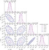 |
Fig. 3. Corner plot showing the posterior distributions from run 2, fitting the RVM to the MeerKAT observed PA variation. |
4. Timing analyses
In total, we have 16 461 ToAs in the dataset, 364 ToAs from the Lovell Telescope data, 4288 ToAs from the NRT, 10 818 ToAs from the GBT, and 991 ToAs from MeerKAT. Timing analyses were made using the tempo22 (Hobbs et al. 2006; Edwards et al. 2006) software package.
The different datasets were combined using an arbitrary phase offset, or ‘JUMP’ between each of them, using the MeerKAT data as the reference dataset. These jumps account for additional time delays due to different backend instruments and geographical locations and are an arbitrary phase offset between each telescope dataset.
All ToAs acquired and generated were first transformed into TT(BIPM2021)3, which is a version of terrestrial time as defined by the International Astronomical Union (IAU). Thereafter, these ToA’s are converted into ToAs at the Solar System barycentre using the DE438 Solar System ephemeris of the Jet Propulsion Laboratory (Park et al. 2021, JPL).
The initial orbital, astrometric and pulsar parameter estimates were found using the ELL1H orbital model implemented in the tempo2 software (Freire & Wex 2010). This model is based on the ELL1 model (Lange et al. 2001), which is designed to avoid the extreme correlation between the epoch of periastron (T0) and the longitude of periastron at T0 (ω) for low-eccentricity orbits, with the xe2 terms (Zhu et al. 2019) added for accuracy; this is especially important for wide systems like J1455−3330.
The ELL1H model mitigates the correlation between the two PK parameters that quantify the Shapiro delay measurement (range, r and shape, s) by re-parameterizing the Shapiro delay with 2 different PK parameters, the orthometric amplitude (h3) and orthometric ratio (ς) (Freire & Wex 2010).
This model, however, is only able to account for the secular variation of the projected semi-major axis (ẋ) and not the full set of kinematic contributions to the variation (see Kopeikin 1995, 1996). The model cannot discriminate between the multiple solutions for the orbital orientation of the system given by the ẋ and inclination angle. Therefore, we also use the T2 orbital model (Edwards et al. 2006), which is based on the DD model (Damour & Deruelle 1986) and self-consistently accounts for all kinematic contributions to the orbital and post-Keplerian parameters. All kinematic contributions to the changes of orbital orientation with respect to our line of sight are calculated internally from the orbital orientation of the system given by the longitude of the ascending node (Ω) and orbital inclination (i). In particular, the T2 model does not separately fit for the variation of the projected semi-major axis of the pulsar’s orbit (ẋ).
To understand and eliminate stochastic noise variations in our dataset, we used the temponest (Lentati et al. 2014) plugin to tempo2, which is a Bayesian parameter estimation tool used to perform non-linear fits of the T2 timing model to the data. We chose the best-fit noise model to describe the data by testing four different noise models. This selection process includes a white-noise only model, a white-noise plus red-noise model, a white-noise plus DM-noise model, and a white-noise plus DM-noise plus red-noise model. In each of these scenarios, a white-noise model is described by EFAC and EQUAD (which scales the uncertainties of the ToAs linearly and quadratically, respectively), a DM-noise model is described by a chromatic power-law model, and a stochastic achromatic power law model describes a red-noise model. For each model, we provide uniform priors centred on the initial best-fit tempo2 parameter ±40 σ, where σ is the associated tempo2 uncertainty. For a select set of parameters, we provided physically motivated priors in two separate temponest runs. This allowed us to explore multiple plausible geometries of the system while avoiding premature convergence to a single local solution. The first run’s Ω was set to cover the range of possible values 0–360° and i was set to cover the range of values 0–90°. The second run’s Ω was set to cover 270–450° (–90–90°), and i was set to cover the range of possible values 90–180°. The parallax, ϖ, was set to range from 0.3 to 3, and Mc from 0.1 to 1.4 M⊙ for both temponest runs.
We performed comparisons between the models using the Nested Importance Sampling Global Log-Evidence and we find the strongest evidence for a white-noise plus DM-noise model. All DM effects are well-modelled by including the DM1 and DM2 timing parameters. These parameters describe the coefficients to the first- and second-order DM derivatives and are expressed as a DM Taylor series expansion.
For the remainder of the paper, we use the outcomes of the temponest posterior distributions, which include DM-noise parameters only. The amplitude and power-law spectral index of the DM-noise are provided in Table 4.
A recent investigation of the influence of different timing models on measured parameters of J1455−3330 using the 15 yr NANOGrav dataset (Lam et al. 2025) found a preference for a linear trend in DM plus a fixed solar wind density over a variety of models (DMX model, a linear trend in DM plus a fixed solar wind density, a quadratic trend in DM plus a fixed solar wind density, and a linear trend in DM plus a varying solar wind density). Although the parallax varies across models, the value obtained using the most favoured model agrees with the value obtained from our analyses of the full dataset. Furthermore, we use the time domain realisation methods of the La Forge GitHub repository4 (Shafiq Hazboun 2020) and overplot the resultant realisations on the post-fit timing residuals (without including the DM noise model) as orange lines on the middle panel of Fig. 4. The noise model aligns with the visible trends in the data, further demonstrating the validity of the noise model.
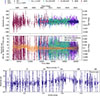 |
Fig. 4. Timing residuals across epochs (top, middle) and orbital phase (bottom). Top: We obtain a weighted rms of 3.201 μs after applying the best-fit values using the T2 timing and noise model described in Sect. 4. Middle: Post-fit timing residuals without subtracting the DM noise model. The time domain realisations of the 100 parameter DM noise model are overlaid as orange lines and the black dots show the median across all the DM model realisations at each ToA. Bottom: MeerKAT residuals as a function of orbital phase, where the orbital phase is measured from the longitude of periastron (ω = 223.47°). Superior conjunction = Tasc + 90°, occurs at orbital phase = 0.63. A Shapiro delay signal is discernible at orbital phase 0.63 when setting Mc = 0 while keeping all other parameters fixed. We overplot the expected theoretical signal based on the best-fit inclination and companion mass values of the full dataset in purple. The line width indicates the 1σ deviations in companion mass and inclination angle. |
5. Results
In this section, we present the complete set of spin, astrometric, binary and derived parameters using the T2 model. These are shown in Table 3. The final temponest solution is a good description of the data and the timing residuals obtained after comparing individual ToAs with the model are shown in Fig. 4. The lack of any visible trends in the residuals and the low weighted rms of ∼3.19 μs further show how well the model fits the data. To visualise the temponest T2 posterior distributions with corner plots, we used the chainconsumer library (Hinton 2016) to plot the 1D and 2D posterior distributions of the measured parameters. Fig. 5 shows the resulting output for a subset of timing parameters of interest. In this plot, we used the DM-noise model in temponest with 5000 live points to produce well-sampled distributions. The dark blue, medium blue and white contours on the 2D off-diagonal plots show the 39%, 86%, and 98% credibility regions respectively. The shaded region on the 1D diagonal plots represents the 68.27% credibility region.
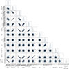 |
Fig. 5. Output posterior distribution for the relevant orbital and post-Keplerian parameter subset of timing parameters for J1455−3330. These were obtained from temponest using the T2 orbital model, which includes a DM-only noise model. The plot was generated using the chainconsumer package. Full details of the parameters are provided in Table 4. The obtained pulsar mass (Mp) distribution was computed using the mass function and the posterior distributions on Mc, i, x, and Pb. The 1D marginalised posterior distributions for each parameter are shown on the diagonal subplots, and the shaded region indicates the 1-σ credibility interval. The 2D contours on the off-diagonal subplots show the correlation between pairs of parameters, where the contours mark the 39%, 86%, and 98% credibility regions respectively. |
J1455−3330 timing parameters obtained from temponest.
Binary timing parameters and associated mass and inclination values for J1455−3330.
We briefly highlight each of the measured and derived parameters in the following subsections. These parameters consist of proper motion, parallax, spin parameters, orbital period derivative (Ṗb), rate of advance of periastron ( ), Shapiro delay, change in projected semi-major axis (ẋ), annual orbital parallax, and finally the constraints on the component masses and 3D orbital geometry.
5.1. Position and proper motion
We provide an updated position and proper motion for J1455−3330. The updated J2000 position obtained from timing is right ascension, α = 14:55:47.973129(2), and declination, δ = −33:30:46.39040(6). From the measured proper motion in right ascension (μα = 7.846(6) mas yr−1) and proper motion in declination (μδ = −2.02(1) mas yr−1), we obtain a total proper motion μT = 8.101(6) mas yr−1. The corresponding position angle of the proper motion, θμ = tan−1(μα/μδ) is 284.42(9)°.
5.2. Parallax
Combining the estimated DM with models of the electron distribution of the Galaxy, we infer a distance to the pulsar between ∼0.527 kpc (Cordes et al. 2002, from the NE2001 model) and ∼0.684 kpc (Yao et al. 2017, from YMW16 model).
In this case, we have a direct measurement of the pulsar parallax, ϖ = 1.11(6) mas, which can be inverted to provide a distance estimate of 0.90(5) kpc. However, this relation is prone to the Lutz-Kelker bias (Lutz & Kelker 1973) where parallax measurements are overestimated because they do not properly account for the larger volume of space that is sampled at smaller parallax values. We correct for this bias using a scaled probability density function. Following Verbiest et al. (2012) and Antoniadis (2021) we infer a probability density function for the distance to the system using:
 (2)
(2)
We assumed that the parallax measurement, ϖ is normally distributed about the true parallax, d−1, with a dispersion σϖ. The e−dPSR/Ld2L−3 term accounts for a Lutz-Kelker bias (Lutz & Kelker 1973, L-K bias) with an exponentially decreasing stellar density almost constant for d ≪ L). L can be considered as a characteristic length scale, which is set to 1.35 kpc following Antoniadis (2021). The estimate of the pulsar distance (dPSR) corrected for the L-K bias from the measured parallax is  kpc.
kpc.
Combining dPSR with μT, we obtained a heliocentric transverse velocity of VT = 34.5 ± 1.9 km s −1.
5.3. Spin parameters
The observed spin period of the pulsar includes both the intrinsic spin period and the kinematic contributions:
 (3)
(3)
where Ṗint is the intrinsic spin-down rate, P is the pulsar’s spin period, Ṗobs is its observed spin-down rate. The kinematic effects are caused by the combined effect of; (1) ṖShk, which is the Shklovskii effect (Shklovskii 1970), and (2) the ṖGal, which is the acceleration of the binary in the gravitational field of the Milky Way due to differential rotation. The Shklovskii effect depends on μT and dPSR as follows:
 (4)
(4)
The Galactic acceleration, (Ṗ/P)Gal, is the difference between the accelerations of the pulsar binary system and the Solar System in the gravitational field of the Galaxy, projected along the line of sight from the Solar System to the pulsar binary system. This Galactic acceleration includes contributions from both the Galactic rotation and vertical accelerations relative to the disk of the Galaxy. Following Damour & Taylor (1991), Nice & Taylor (1995), Lazaridis et al. (2009), and Pathak & Bagchi (2018),
 (5a)
(5a)
 (5b)
(5b)
 (5c)
(5c)
where β = (dPSR/R⊙)cos b − cos l and zkpc = dPSR|sin b| in kpc. R⊙ = 8.28(3) kpc is the distance to the Galactic centre, and Ω⊙ = 241(4) km s−1 is the Galactic rotation velocity (GRAVITY Collaboration 2021; Guo et al. 2021). Kz/c is the vertical component of Galactic acceleration, and is given by McMillan (2017):
![Mathematical equation: $$ \begin{aligned} \frac{K_z}{c} \left[s^{-1}\right] = -1.08\times 10^{-19}\left( 0.58 + \frac{1.25}{(z_{\rm {kpc}}^{2}+0.0324)^{1/2}} \right) z_{\rm {kpc}}. \end{aligned} $$](/articles/aa/full_html/2026/04/aa56766-25/aa56766-25-eq25.gif) (6)
(6)
Using the distance estimated from parallax, the Shklovskii effect (Ṗ/P)Shk is 1.15(7)×10−21 s−1 and the Galactic acceleration (Ṗ/P)Gal is 6.8(3)×10−22 s−1. Subtracting these two terms from Ṗobs = 2.430 × 10⁻²⁰ s s−1 we obtain the ‘intrinsic’ variation in the spin period, Ṗint = 2.25(1) × 10−20 s s−1. This intrinsic spin-down value is very close to the observed spin-down since the Shklovskii and Galactic terms are ∼10–100 times smaller. Using this Ṗint, we estimated the surface magnetic field (Bs = 4.230(9)×108G), the characteristic age (τc = 5.63(3) Gyr), and the spin-down luminosity of the system (Ė = 1736(8) 1030 erg s−1, Lorimer & Kramer 2004).
5.4. Binary period derivative: Ṗb
Using the current timing baseline, we did not obtain a significant detection of the orbital period derivative (Ṗb = 9(7) × 10−13 s s−1). The expected contributions to Ṗb are:
 (7)
(7)
where  is the observed orbital period derivative,
  is the contribution due to gravitational wave decay,
  and
and  are the same kinematic contributions described in Sect. 5.3,
  is the mass loss in the system, and
  is the tidal dissipation of the orbit. We find that the only non-negligible contribution arises from the kinematic terms.
From Equations (4), (5), and (6), we obtain the following results: Ṗb,Shk = 9.5(5)×10−13 s s−1 and Ṗb,Gal = 5.6(3)×10−13 s s−1. In Fig. 6, we can see how these quantities and their sum change as a function of the distance.
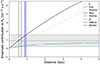 |
Fig. 6. Kinematic contributions to Ṗb as a function of distance. The distance constraints from ϖ, the NE2001 model, and the YMW16 model are shown as vertical lines. The constraint from Ṗb,obs is shown as the grey shaded region. The curves show the contributions from the vertical and horizontal acceleration from the Galactic disc, the proper motion of the system, and the total acceleration. |
The observed Ṗb is given by Ṗb,obs = 9(7) × 10−13 s s−1, this is shown in Fig. 6 as the grey bar. Within the ±1–σ uncertainties, this matches well the sum of kinematic terms expected for the distance as measured via parallax. As we can see in the figure, the steepness of the curve of the total kinematic effects implies that a more precise value of Ṗobs will also provide an independent estimate of the distance, which can be compared with the parallax distance.
The intrinsic Ṗb is given by Ṗb,int = Ṗb,obs- Ṗb,Skk − Ṗb,Gal = −6(7) × 10−13 s s−1. This is expected to originate from the orbital decay of the system caused by gravitational wave emission. Using the orbital parameters, masses (derived from the T2 model) and the relation from Peters (1964), we estimate the orbital decay caused by the emission of quadrupolar gravitational waves in GR,  . This is five orders of magnitude below the current timing precision, i.e. within measurement precision it is expected to be consistent with zero, as observed.
5.5. Rate of advance of periastron: 
The very low significance  = 1.5(1.3)×10−3 deg yr−1 measured with the T2 model, can still be used as an upper limit for the total mass of the system.
When GR is assumed, the  can be described using the Keplerian parameters and total mass of the system as
 (8)
(8)
Using the masses obtained from the T2 model, we obtain a prediction of  . The observed value is consistent with this expectation but is not yet precise enough to usefully constrain the masses (see Fig. 7).
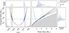 |
Fig. 7. Constraints on the companion mass as a function of the cosine of the orbital inclination (left), and as a function of the pulsar mass (right). In the left plot, the grey region is excluded by the requirement that the pulsar mass must be greater than zero. In the right plot, the mass values in the grey region are excluded by the mass function. The black solid and dashed lines and the pink solid and dashed lines represent the median, and 1 sigma ς and h3 measurements using the ELL1H model respectively. The solid contours enclosing progressively darker shades of purple include 98%, 86%, and 39% confidence limits of the 2D probability density function from the T2 timing model solutions calculated by temponest with priors of i ranging from 90 to 180 degrees and Ω ranging from 270 to 450 degrees. The solid contours enclosing progressively darker shades of purple include 98%, 86%, and 39% confidence limit of the 2D probability density function from the T2 timing model solutions calculated by temponest with priors of i ranging from 0 to 90 degrees and Ω ranging from 0 to 360 degrees. The marginalised posterior probability distributions for cos i, Mc and Mp are displayed for each axis. The shaded region on the marginalised plots at the top and the right represents the 68% confidence limit of the estimated parameter. |
5.6. Shapiro delay
As seen in Fig. 4, the Shapiro delay signal, which describes the relativistic light-propagation delay in the system, has a maximum of ∼ 9 μs using the MeerKAT data. This low amplitude is a consequence of a more face-on configuration of the system, and one of the reasons why this delay was not detected until now. Using the ELL1H model, we have found a significant detection of  μs and an orthometric ratio
  . These constraints are displayed in Fig. 7.
5.7. Change in projected semi-major axis: ẋ
Using the ELL1H model, we measure a highly significant  s s−1. This measurement is fully consistent with the value presented by EPTA Collaboration (2023) but is 3 times more precise, going from a ∼33 sigma detection to a ∼ 100 sigma detection; an improvement due to the inclusion of the MeerKAT data. This ẋ can be the result of various effects and is summarised as follows:
 (9)
(9)
where the contributions to the observed ẋ are due to the emission of gravitational waves (GW), proper motion of the binary system (μ), varying aberration, dεA/dt, changing Doppler shift  , spin–orbit coupling and a hypothetical third companion (planet) around the pulsar.
A detailed calculation shows that only the secular variation of x caused by the proper motion (ẋ/xpm, Kopeikin 1996) contributes significantly to the observed ẋ. The term arises because our viewing angle of the binary (i) keeps changing due to its proper motion. The effect on x = ap sin i/c is given by
 (10)
(10)
The constraints derived from ẋ on the orbital orientation of the system can be seen as dotted lines in Fig. 8.
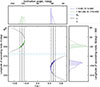 |
Fig. 8. Plot of the allowable orbital orientation of J1455−3330. The black lines represent constraints from ς, and grey contours show the constraint from ẋ (1-σ solid, 3-σ dashed). The green dashed contours show the constraints from temponest using priors where the inclination angle ranges from 90 to 180 and Ω ranges from 270 to 450 (–90–90°). The purple dashed contours show the constraints from temponest using priors where inclination angle, i, ranges from 0 to 90 and longitude of ascending node Ω ranges from 0 to 360. The light blue dashed horizontal line shows the position angle of the proper motion. The marginalised constraints on cos i and Ω are shown as 1D histograms (in green and purple) in the top and side panels. |
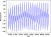 |
Fig. 9. Simulated estimates of the peak-to-peak amplitude of the AOP for J1455−3330 (∼400 ns). Our precision on xp ∼ 0.4 μs. Therefore, the AOP signal is undetectable above the timing noise. |
5.8. Annual orbital parallax
As the Earth orbits the Sun, a binary system is observed at slightly different angles, which can be seen as a periodic change in the apparent inclination angle (and thus of x = ap sin i) of the pulsar orbit. For nearby binary systems, this effect is known as the annual orbital parallax (Kopeikin 1995), and can cause a measurable variation of the projected semi-major axis. Following Kopeikin (1995), this cyclic effect can be expressed as,
 (11)
(11)
where c is the speed of light, d is the distance between the binary and the Solar System barycentre (SSB), and K0 is the unit normal vector pointing from the SSB to the barycentre of the binary. The vectors r = (X, Y, Z) and rp are the Earth’s position with respect to the SSB and the pulsar position with respect to the SSB, which depend on the Solar System ephemeris model that is used and varies with time. Following Geyer et al. (2023), we estimate the expected peak-to-peak amplitude of the annual orbital parallax (AOP) by assuming that both the pulsar’s binary orbit and Earth’s orbit are circular (e = 0). We used
![Mathematical equation: $$ \begin{aligned} \begin{aligned} \Delta _\pi = \frac{x_{\rm p}}{d_{\rm {PSR}}} \Bigl [ (\Delta _{\rm I0} \sin {\Omega } - \Delta _{\rm J0} \cos {\Omega }) \sin {\omega _{\rm {Pb}} t} \cot {i} \\ - (\Delta _{\rm I0} \cos {\Omega } + \Delta _{\rm J0} \sin {\Omega }) \cos {\omega _{\rm {Pb}} t} \csc {i} \Bigr ] \end{aligned} \end{aligned} $$](/articles/aa/full_html/2026/04/aa56766-25/aa56766-25-eq46.gif) (12)
(12)
where xp is the projected semi-major axis, Ω is the longitude of the ascending node, i is the inclination angle of the system, and ωPb = 2π/Pb is the binary orbital frequency. This effect may be prominent in J1455−3330 since the projected semi-major axis, xp = 32.3622059(4) s, is large, and the system is relatively close to the Earth (∼ 0.90(5) kpc).
Measuring this effect will help break the degeneracy in the 3D orbital geometry of the system that results, in Fig 8 from the multiple intersections of the ς and ẋ lines. The unit vectors (I0, J0, K0) describe the coordinate system of the pulsar reference frame, with its origin at the binary system barycentre. Following Kopeikin (1995),
 (13)
(13)
 (14)
(14)
where α and δ are the pulsar’s right ascension and declination, and r = (X, Y, Z) is the Earth’s position with respect to the SSB described before. We obtain the Earth’s (X, Y, Z) coordinates as a function of our observing MJD range using the same JPL solar ephemeris as in our timing results (DE438), which is contained within the jplephem package and implemented in astropy. We note that Kopeikin (1995) generally follows the coordinate system of DT92, and the relevant angles need to be transformed accordingly to agree with the observer’s convention used throughout this paper. We compute the resulting Δπ oscillatory trend as a function of MJD and find a peak-to-peak orbital parallax of ϖ ∼ 400 ns. Therefore, the AOP signal is undetectable above the timing noise.
5.9. Self-consistent estimates of masses and orbital orientation
We now use all the effects we have been discussing until now in a self-consistent way to determine the masses of the pulsar, of the companion and the orbital orientation using temponest. The resulting constraints placed on Mc, cos i, and Mp are shown in Fig. 7 as probability contours, the constraints on cos i and Ω are shown in Fig. 8.
The probability density contours for each of the islands show that two distinct regions in the Mc–Mp plane and in the cos i – Ω plane are preferred. In all subplots of these Figures, the purple and green contours are given by the two separate temponest runs. TN run 1 has priors on i:0–90° and Ω:0–360°, and TN run 2 i:90–180° and Ω:270–450°. For the first run, we estimate  ,
,  , i = 63(2)° and Ω = 212(12)°. For the second run we estimate
  ,
,  , and i = 123(4)° and Ω = 334(12)°.
In Fig. 7, we see how the masses allowed by the temponest runs follow the h3 and ς constraints determined in the ELL1H solution. Although of low significance, the  constraints might in the near future set an upper limit on Mp, excluding the large tail portion of the probability density contours.
Similarly, in Fig. 8, we see how the orbital orientations allowed by the temponest runs follow closely the ẋ curve and ς constraints derived from the ELL1H model ς. In this figure, we also see that the annual orbital parallax strongly disfavours values of Ω that are more than 90 degrees away from the proper motion. At the moment, those are not taken into account given the very low statistical significance of  . In both analyses, the higher probability island includes the prior region i:0–90° and Ω:0–360°; the maximum likelihood of which are enclosed by purple contours in Fig. 7 and Fig. 8.
6. Discussion and conclusions
In this paper, we have presented the results of our timing analyses of J1455−3330 by combining available Lovell, NRT, Green Bank, and MeerKAT data with a total timing baseline of ∼30 years. The results include precise astrometry and parallax measurements, several kinematic effects, and a first measurement of its Shapiro delay.
A detailed analysis of the above relativistic effects has resulted in two solutions of the system’s component masses and orbital orientation. Assuming general relativity we find two solutions: (1) a pulsar mass  , a companion mass
  , an orbital inclination, i = 63(2)°, and longitude of the ascending node, Ω = 212(12)° or (2) a pulsar mass Mp =
  M⊙, a companion mass Mc = 0.309
 M⊙, an orbital inclination, i = 123(4)°, and longitude of the ascending node, Ω = 334(12)°. The mass measurements and orbital geometry of the system from both temponest runs are consistent. The best fit RVM model resulted in α = 105.0(9), and ζ′ = 112.4(9), which translates to i ∼ 180 − ζ′ = 61.6(9).
The companion mass in the higher probability island,  M⊙, is consistent with a HeWD companion mass predicted by the Tauris & Savonije (1999) relation where the uncertainty on the measured companion mass (∼0.046 M⊙), gives a companion mass ranging from 0.247 M⊙ to 0.339 M⊙. In Fig. 7, the lower, middle, and upper dashed light blue lines correspond to the predictions of Mc for Population I progenitors (corresponding to a metallicity of Z = 0.02), Population II progenitors (Z = 0.001), and Population I+II progenitors. For an orbital period of ∼ 76.17 days, the Tauris & Savonije (1999) relation predicts Mc ∼ 0.315 M⊙ given a Population I progenitor, Mc = 0.348 M⊙ given a Population II progenitor, and Mc = 0.331 M⊙ given a Population I+II progenitor. A previous study regarding wide-orbit binary MSPs suggested that the Tauris & Savonije (1999) relation may overestimate the WD masses (Stairs et al. 2005). This study focused on binaries that did not contain precise mass measurements, and J1455−3330 is an example of a wide orbit binary whose estimated companion mass is in agreement with the Tauris & Savonije (1999) relation.
The measured pulsar mass in the higher probability island,  , lies within 1σ of the peak of the birth mass distribution proposed by You et al. (2025). You et al. (2025) found that the neutron star birth mass function can be described as a turn-on power law model that has a minimum mass of
  and a maximum mass of
  . The distribution peaks at
  and declines with a power-law index of
  . Electron-capture supernovae are likely to produce neutron stars with masses around the peak of the distribution, like J1455−3330.
The eccentricity of 1.6×10⁻⁴ agrees well with the theoretical range predicted by Phinney & Kulkarni (1994) for a MSP HeWD binary with an orbital period of ∼76.17 days. The mass measurements, eccentricity, Tauris & Savonije (1999) relation and Phinney & Kulkarni (1994) relation, suggest that the system followed a standard evolutionary path, where the system is likely formed from wide-orbit low-mass X-ray binaries.
The advance of periastron predicted by GR,  , and our fit for this parameter yields
  . After ∼30 years of timing data, its uncertainty is still around two times larger than the expected effect (see Fig. 10). However, measuring this parameter should be feasible in the not-too-distant future with continued timing with MeerKAT and SKA observations.
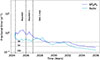 |
Fig. 10. Improvement in the fractional error of orbital period decay, Ṗb, and |


Indeed, simulated ToAs for J1455−3330 using knowledge of the sensitivity of current and future telescopes suggest a 3σ detection of  around 2029 and a 3σ detection of Ṗb around 2032. We assume future observing plans using the best telescopes for observing this pulsar, i.e. MeerKAT, MeerKAT+ and SKA 1-mid. We scale our ToA uncertainties for MeerKAT+ and SKA 1-mid based on our current ToA uncertainties measured with MeerKAT, and adopt an observing cadence of once every 7 days for MeerKAT and MeerKAT+, and once every 14 days for SKA 1-mid. A precise
  measurement will result in a much more precise constraint on the component masses, and a measurement of Ṗb will provide an independent estimate of the distance to the system.
Mass measurements of pulsars and companions in binary systems are important for the study of EoS, binary evolution theories, and they allow us to test key correlations such as the Tauris & Savonije (1999) relation. The mass constraints of PSR J1455−3330, presented in this study, have provided another data point to the growing population of measured neutron star masses, the study of which will eventually help us identify the maximum possible mass of a neutron star and unveil more about the NS mass distribution itself.
Acknowledgments
We thank the anonymous referee for the helpful comments and suggestions. The MeerKAT telescope is operated by the South African Radio Astronomy Observatory, which is a facility of the National Research Foundation, an agency of the Department of Science and Innovation. SARAO acknowledges the ongoing advice and calibration of GPS systems by the National Metrology Institute of South Africa (NMISA) and the time space reference systems department of the Paris Observatory. MeerTime data is housed on the O-zSTAR supercomputer at Swinburne University of Technology maintained by the Gravitational Wave Data Centre and ADACS via NCRIS support. Pulsar research at the Jodrell Bank Centre for Astrophysics and the observations using the Lovell Telescope are supported by a Consolidated Grant (ST/T000414/1) from the UK’s Science and Technology Facilities Council (STFC). The Nançay Radio Observatory is operated by the Paris Observatory, associated with the French Centre National de la Recherche Scientifique (CNRS). We acknowledge financial support from the “Action Thématique de Cosmologie et Galaxies” (ATCG), “Action Thématique Gravitation Références Astronomie Métrologie” (ATGRAM) and “Action Thématique Phénomènes Extrêmes et Multi-messagers” (ATPEM) of CNRS/INSU, France. The Green Bank Observatory is a facility of the NSF operated under cooperative agreement by Associated Universities, Inc. This research has made extensive use of NASA’s Astrophysics Data System (https://ui.adsabs.harvard.edu/). The analysis done in this publication made use of the open source pulsar analysis packages psrchive Hotan et al. (2004), tempo2 Hobbs et al. (2006) and temponest Lentati et al. (2014), as well as open source Python libraries including Numpy, Matplotlib, Astropy and Chainconsumer. The authors thank T. Dolch, M. T. Lam, and E. Fonseca for their valuable comments, which helped improve this work. D.S.P. and V.V.K. acknowledge continuing valuable support from the Max Planck Society. D.S.P. acknowledges support from the International Max Planck Research School (IMPRS) for Astronomy and Astrophysics at the University of Bonn and University of Cologne. V.V.K. acknowledges financial support from the ERC starting grant ‘COMPACT’ (Understanding gravity using a COMprehensive search for fast-spinning Pulsars And CompacT binaries, grant agreement no. 101078094). J.S. acknowledges the support from the University of Cape Town Vice Chancellor’s Future Leaders 2030 Awards programme and the South African Research Chairs Initiative of the Department of Science and Technology and the National Research Foundation. R.M.S. acknowledges support Australian Research Council Future Fellowship FT190100155, and the Australian Research Council Centre of Excellence for Gravitational Wave Discovery (CE170100004 and CE230100016.)
References
- Agazie, G., Alam, M. F., Anumarlapudi, A., et al. 2023, ApJ, 951, L9 [CrossRef] [Google Scholar]
- Alpar, M. A., Cheng, A. F., Ruderman, M. A., & Shaham, J. 1982, Nature, 300, 728 [NASA ADS] [CrossRef] [Google Scholar]
- Antoniadis, J. 2021, MNRAS, 501, 1116 [Google Scholar]
- Bailes, M., Jameson, A., Abbate, F., et al. 2020, PASA, 37, e028 [NASA ADS] [CrossRef] [Google Scholar]
- Cordes, J. M., Lazio, T. J. W., Chatterjee, S., Arzoumanian, Z., & Chernoff, D. 2002, in 34th COSPAR Scientific Assembly, 34, 2305 [Google Scholar]
- Damour, T., & Deruelle, N. 1986, Ann. L’Institut Henri Poincare Section (A) Phys. Theorique, 44, 263 [Google Scholar]
- Damour, T., & Taylor, J. H. 1991, ApJ, 366, 501 [NASA ADS] [CrossRef] [Google Scholar]
- Desvignes, G., Caballero, R. N., Lentati, L., et al. 2016, MNRAS, 458, 3341 [Google Scholar]
- Edwards, R. T., Hobbs, G. B., & Manchester, R. N. 2006, MNRAS, 372, 1549 [Google Scholar]
- EPTA Collaboration (Antoniadis, J., et al.) 2023, A&A, 678, A48 [Google Scholar]
- Fonseca, E., Cromartie, H. T., Pennucci, T. T., et al. 2021, ApJ, 915, L12 [NASA ADS] [CrossRef] [Google Scholar]
- Freire, P. C. C., & Wex, N. 2010, MNRAS, 409, 199 [NASA ADS] [CrossRef] [Google Scholar]
- Gangadhara, R. T. 1997, A&A, 327, 155 [NASA ADS] [Google Scholar]
- Geyer, M., Venkatraman Krishnan, V., Freire, P. C. C., et al. 2023, A&A, 674, A169 [NASA ADS] [CrossRef] [EDP Sciences] [Google Scholar]
- GRAVITY Collaboration (Abuter, R., et al.) 2021, A&A, 647, A59 [NASA ADS] [CrossRef] [EDP Sciences] [Google Scholar]
- Guillemot, L., Cognard, I., van Straten, W., Theureau, G., & Gérard, E. 2023, A&A, 678, A79 [NASA ADS] [CrossRef] [EDP Sciences] [Google Scholar]
- Guo, Y. J., Freire, P. C. C., Guillemot, L., et al. 2021, A&A, 654, A16 [NASA ADS] [CrossRef] [EDP Sciences] [Google Scholar]
- Hinton, S. R. 2016, J. Open Source Software, 1, 00045 [NASA ADS] [CrossRef] [Google Scholar]
- Hobbs, G., Lyne, A. G., Kramer, M., Martin, C. E., & Jordan, C. 2004, MNRAS, 353, 1311 [NASA ADS] [CrossRef] [Google Scholar]
- Hobbs, G. B., Edwards, R. T., & Manchester, R. N. 2006, MNRAS, 369, 655 [Google Scholar]
- Hotan, A. W., van Straten, W., & Manchester, R. N. 2004, PASA, 21, 302 [Google Scholar]
- Johnston, S., & Kramer, M. 2019, MNRAS, 490, 4565 [NASA ADS] [CrossRef] [Google Scholar]
- Kopeikin, S. M. 1995, ApJ, 439, L5 [NASA ADS] [CrossRef] [Google Scholar]
- Kopeikin, S. M. 1996, ApJ, 467, L93 [NASA ADS] [CrossRef] [Google Scholar]
- Kramer, M., & Johnston, S. 2025, MNRAS, in press [arXiv:2510.05778] [Google Scholar]
- Kramer, M., Stairs, I. H., Venkatraman Krishnan, V., et al. 2021, MNRAS, 504, 2094 [CrossRef] [Google Scholar]
- Lam, M. T., Kaplan, D. L., Agazie, G., et al. 2025, AAS, submitted [arXiv:2506.03597] [Google Scholar]
- Lange, C., Camilo, F., Wex, N., et al. 2001, MNRAS, 326, 274 [NASA ADS] [CrossRef] [Google Scholar]
- Lazaridis, K., Wex, N., Jessner, A., et al. 2009, MNRAS, 400, 805 [NASA ADS] [CrossRef] [Google Scholar]
- Lazarus, P., Karuppusamy, R., Graikou, E., et al. 2016, MNRAS, 458, 868 [Google Scholar]
- Lentati, L., Alexander, P., Hobson, M. P., et al. 2014, MNRAS, 437, 3004 [NASA ADS] [CrossRef] [Google Scholar]
- Lorimer, D. R., & Kramer, M. 2004, in Handbook of Pulsar Astronomy (Cambridge University Press) [Google Scholar]
- Lorimer, D. R., Nicastro, L., Lyne, A. G., et al. 1995, ApJ, 439, 933 [NASA ADS] [CrossRef] [Google Scholar]
- Lutz, T. E., & Kelker, D. H. 1973, PASP, 85, 573 [Google Scholar]
- Manchester, R. N. 1975, PASA, 2, 334 [NASA ADS] [CrossRef] [Google Scholar]
- Martinez, J. G., Stovall, K., Freire, P. C. C., et al. 2015, ApJ, 812, 143 [NASA ADS] [CrossRef] [Google Scholar]
- McMillan, P. J. 2017, MNRAS, 465, 76 [NASA ADS] [CrossRef] [Google Scholar]
- Nice, D. J., & Taylor, J. H. 1995, ApJ, 441, 429 [NASA ADS] [CrossRef] [Google Scholar]
- Park, R. S., Folkner, W. M., Williams, J. G., & Boggs, D. H. 2021, AJ, 161, 105 [NASA ADS] [CrossRef] [Google Scholar]
- Pathak, D., & Bagchi, M. 2018, ApJ, 868, 123 [NASA ADS] [CrossRef] [Google Scholar]
- Peters, P. C. 1964, Phys. Rev., 136, 1224 [Google Scholar]
- Phinney, E. S. 1992, Philos. Trans. Royal Soc. London Ser. A, 341, 39 [Google Scholar]
- Phinney, E. S., & Kulkarni, S. R. 1994, ARA&A, 32, 591 [NASA ADS] [CrossRef] [Google Scholar]
- Radhakrishnan, V., & Cooke, D. J. 1969, Astrophys. Lett., 3, 225 [NASA ADS] [Google Scholar]
- Radhakrishnan, V., & Srinivasan, G. 1982, Curr. Sci., 51, 1096 [NASA ADS] [Google Scholar]
- Serylak, M., Johnston, S., Kramer, M., et al. 2021, MNRAS, 505, 4483 [NASA ADS] [CrossRef] [Google Scholar]
- Serylak, M., Venkatraman Krishnan, V., Freire, P. C. C., et al. 2022, A&A, 665, A53 [NASA ADS] [CrossRef] [EDP Sciences] [Google Scholar]
- Shafiq Hazboun, J. 2020, https://doi.org/10.5281/zenodo.4152550 [Google Scholar]
- Shklovskii, I. S. 1970, Sov. Ast., 13, 562 [Google Scholar]
- Spiewak, R., Bailes, M., Miles, M. T., et al. 2022, PASA, 39, e027 [NASA ADS] [CrossRef] [Google Scholar]
- Stairs, I. H., Faulkner, A. J., Lyne, A. G., et al. 2005, ApJ, 632, 1060 [NASA ADS] [CrossRef] [Google Scholar]
- Tauris, T. M., & Savonije, G. J. 1999, A&A, 350, 928 [NASA ADS] [Google Scholar]
- Tauris, T. M., & van den Heuvel, E. P. J. 2023, Physics of Binary Star Evolution. From Stars to X-ray Binaries and Gravitational Wave Sources [Google Scholar]
- van Straten, W. 2004, ApJS, 152, 129 [NASA ADS] [CrossRef] [Google Scholar]
- van Straten, W. 2006, ApJ, 642, 1004 [NASA ADS] [CrossRef] [Google Scholar]
- van Straten, W. 2013, ApJS, 204, 13 [NASA ADS] [CrossRef] [Google Scholar]
- Verbiest, J. P. W., Weisberg, J. M., Chael, A. A., Lee, K. J., & Lorimer, D. R. 2012, ApJ, 755, 39 [NASA ADS] [CrossRef] [Google Scholar]
- Yao, J. M., Manchester, R. N., & Wang, N. 2017, ApJ, 835, 29 [NASA ADS] [CrossRef] [Google Scholar]
- You, Z.-Q., Zhu, X., Liu, X., et al. 2025, Nat. Astron., 9, 552 [Google Scholar]
- Zhu, W. W., Desvignes, G., Wex, N., et al. 2019, MNRAS, 482, 3249 [NASA ADS] [CrossRef] [Google Scholar]
All Tables
α and ζ′ priors and posteriors, log likelihood, and implied inclination angle, i, for six different RVM model fits.
Binary timing parameters and associated mass and inclination values for J1455−3330.
All Figures
|
Fig. 1. Definition of angles and conventions used in this paper. Throughout this paper, we adopt the ‘observer’s convention’ for all geometric quantities. The fundamental reference plane is in green, and the orbital plane is in purple, with the corresponding unit vectors coloured the same way. S denotes the spin angular momentum, which is aligned with the orbital angular momentum. The magnetic axis (μ) is misaligned from S by the misalignment angle α. The pulsar emission cone has an opening angle ρ, and is cut through by our line of sight at an impact angle β. ζ = α + β is the latitude of the spin axis, which is the same as the orbital inclination angle (i) for spin-aligned systems. |
| In the text | |
|
Fig. 2. Polarisation profile of J1455−3330 obtained from integrating 32.2 hours of observations with the MeerKAT L-band receiver. The black, red, and blue lines in the top panel indicate the total intensity, linear polarisation fraction, and circular polarisation fraction, respectively. The middle panel shows the evolution of the PA across the pulsar’s phase. The PA exhibits the characteristic swing as well as some phase jumps. The red solid line corresponds to the RVM fit to the PA, and the dashed line shows the RVM solution separated by 90° from the main fit to include the jumped PA values (blue dots). The bottom panel shows the PA residuals. |
| In the text | |
|
Fig. 3. Corner plot showing the posterior distributions from run 2, fitting the RVM to the MeerKAT observed PA variation. |
| In the text | |
|
Fig. 4. Timing residuals across epochs (top, middle) and orbital phase (bottom). Top: We obtain a weighted rms of 3.201 μs after applying the best-fit values using the T2 timing and noise model described in Sect. 4. Middle: Post-fit timing residuals without subtracting the DM noise model. The time domain realisations of the 100 parameter DM noise model are overlaid as orange lines and the black dots show the median across all the DM model realisations at each ToA. Bottom: MeerKAT residuals as a function of orbital phase, where the orbital phase is measured from the longitude of periastron (ω = 223.47°). Superior conjunction = Tasc + 90°, occurs at orbital phase = 0.63. A Shapiro delay signal is discernible at orbital phase 0.63 when setting Mc = 0 while keeping all other parameters fixed. We overplot the expected theoretical signal based on the best-fit inclination and companion mass values of the full dataset in purple. The line width indicates the 1σ deviations in companion mass and inclination angle. |
| In the text | |
|
Fig. 5. Output posterior distribution for the relevant orbital and post-Keplerian parameter subset of timing parameters for J1455−3330. These were obtained from temponest using the T2 orbital model, which includes a DM-only noise model. The plot was generated using the chainconsumer package. Full details of the parameters are provided in Table 4. The obtained pulsar mass (Mp) distribution was computed using the mass function and the posterior distributions on Mc, i, x, and Pb. The 1D marginalised posterior distributions for each parameter are shown on the diagonal subplots, and the shaded region indicates the 1-σ credibility interval. The 2D contours on the off-diagonal subplots show the correlation between pairs of parameters, where the contours mark the 39%, 86%, and 98% credibility regions respectively. |
| In the text | |
|
Fig. 6. Kinematic contributions to Ṗb as a function of distance. The distance constraints from ϖ, the NE2001 model, and the YMW16 model are shown as vertical lines. The constraint from Ṗb,obs is shown as the grey shaded region. The curves show the contributions from the vertical and horizontal acceleration from the Galactic disc, the proper motion of the system, and the total acceleration. |
| In the text | |
|
Fig. 7. Constraints on the companion mass as a function of the cosine of the orbital inclination (left), and as a function of the pulsar mass (right). In the left plot, the grey region is excluded by the requirement that the pulsar mass must be greater than zero. In the right plot, the mass values in the grey region are excluded by the mass function. The black solid and dashed lines and the pink solid and dashed lines represent the median, and 1 sigma ς and h3 measurements using the ELL1H model respectively. The solid contours enclosing progressively darker shades of purple include 98%, 86%, and 39% confidence limits of the 2D probability density function from the T2 timing model solutions calculated by temponest with priors of i ranging from 90 to 180 degrees and Ω ranging from 270 to 450 degrees. The solid contours enclosing progressively darker shades of purple include 98%, 86%, and 39% confidence limit of the 2D probability density function from the T2 timing model solutions calculated by temponest with priors of i ranging from 0 to 90 degrees and Ω ranging from 0 to 360 degrees. The marginalised posterior probability distributions for cos i, Mc and Mp are displayed for each axis. The shaded region on the marginalised plots at the top and the right represents the 68% confidence limit of the estimated parameter. |
| In the text | |
|
Fig. 8. Plot of the allowable orbital orientation of J1455−3330. The black lines represent constraints from ς, and grey contours show the constraint from ẋ (1-σ solid, 3-σ dashed). The green dashed contours show the constraints from temponest using priors where the inclination angle ranges from 90 to 180 and Ω ranges from 270 to 450 (–90–90°). The purple dashed contours show the constraints from temponest using priors where inclination angle, i, ranges from 0 to 90 and longitude of ascending node Ω ranges from 0 to 360. The light blue dashed horizontal line shows the position angle of the proper motion. The marginalised constraints on cos i and Ω are shown as 1D histograms (in green and purple) in the top and side panels. |
| In the text | |
|
Fig. 9. Simulated estimates of the peak-to-peak amplitude of the AOP for J1455−3330 (∼400 ns). Our precision on xp ∼ 0.4 μs. Therefore, the AOP signal is undetectable above the timing noise. |
| In the text | |
|
Fig. 10. Improvement in the fractional error of orbital period decay, Ṗb, and |
| In the text | |
Current usage metrics show cumulative count of Article Views (full-text article views including HTML views, PDF and ePub downloads, according to the available data) and Abstracts Views on Vision4Press platform.
Data correspond to usage on the plateform after 2015. The current usage metrics is available 48-96 hours after online publication and is updated daily on week days.
Initial download of the metrics may take a while.