| Issue |
A&A
Volume 708, April 2026
|
|
|---|---|---|
| Article Number | A247 | |
| Number of page(s) | 16 | |
| Section | Extragalactic astronomy | |
| DOI | https://doi.org/10.1051/0004-6361/202557154 | |
| Published online | 10 April 2026 | |
Black hole mass estimation through accretion disk spectral fitting for high-redshift blazars
1
Department of Physics, National and Kapodistrian University of Athens, University Campus Zografos, GR 15784 Athens, Greece
2
Institute of Accelerating Systems & Applications, University Campus Zografos, Athens, Greece
★ Corresponding authors: This email address is being protected from spambots. You need JavaScript enabled to view it.
; This email address is being protected from spambots. You need JavaScript enabled to view it.
Received:
8
September
2025
Accepted:
16
January
2026
Abstract
Context. High-redshift (z > 2) blazars, with relativistic jets aligned toward us, probe the most powerful end of the active galactic nuclei (AGNs) population.
Aims. We aimed to determine the black hole masses and mass accretion rates of high-z blazars in a common framework that utilizes a Markov chain Monte Carlo (MCMC) fitting method and the Shakura-Sunayev multi-temperature accretion disk model, accounting also for attenuation due to neutral hydrogen gas in the intergalactic medium (IGM).
Methods. We compiled a sample of 23 high-redshift blazars from the literature with publicly available infrared-to-ultraviolet photometric data. We performed a Bayesian fit to the spectral energy distribution (SED) of the accretion disk, accounting for upper limits, and determined the black hole masses and mass accretion rates with their uncertainties. We also examined the impact of optical-ultraviolet attenuation due to gas in the IGM.
Results. We find that neglecting IGM attenuation in SED fits leads to systematically larger black hole mass estimates and correspondingly lower Eddington ratios, with the bias becoming more severe at higher redshift. Our MCMC fits yield median black hole masses in the range ∼(108 − 1010) M⊙ and a broad distribution of median Eddington ratios (λEdd ∼ 0.04 up to ∼1), with several objects accreting at λEdd ≳ 0.4 both at z ∼ 2 − 3 and at z ≳ 5. Comparison with previous literature shows no clear method-dependent systematic offsets, although individual mass estimates can differ by up to a factor of a few. We also demonstrate that assumptions about black hole spin introduce a systematic degeneracy, changing the inferred MBH and Ṁ by factors up to five.
Conclusions. This work is, to our knowledge, the first systematic study to model the accretion-disk emission of a large sample of high-z blazars within a single, consistent statistical framework. Our results emphasize the importance of accounting for IGM attenuation and of using uniform fitting methods when comparing disk-based black hole estimates across samples.
Key words: accretion / accretion disks / galaxies: active / quasars: supermassive black holes
© The Authors 2026
 Open Access article, published by EDP Sciences, under the terms of the Creative Commons Attribution License (https://creativecommons.org/licenses/by/4.0), which permits unrestricted use, distribution, and reproduction in any medium, provided the original work is properly cited.
This article is published in open access under the Subscribe to Open model. This email address is being protected from spambots. You need JavaScript enabled to view it. to support open access publication.
1. Introduction
Blazars are active galactic nuclei (AGNs) whose relativistic plasma jets are oriented at small angles to our line of sight. They display broadband, nonthermal emission extending from radio frequencies to very high-energy gamma rays. This radiation, produced by processes such as synchrotron emission and inverse Compton scattering within the jet, forms a characteristic spectral energy distribution (SED) with two broad components: a low-energy hump peaking between the infrared (IR) and X-ray frequencies and a high-energy hump peaking in the gamma-ray regime (for a recent review, see Hovatta & Lindfors 2019).
The central engine powering a blazar is essentially an accretion disk that channels plasma and magnetic flux to a supermassive black hole with mass MBH in the range 107 M⊙ and 1011 M⊙. For accretion rates above a critical threshold, ṁc ∼ 0.03 (Narayan & Yi 1995), the flow is well described by a geometrically thin, radiatively efficient disk model (Shakura & Sunyaev 1973; Novikov & Thorne 1973). Here, the dimensionless accretion rate is defined as ṁ ≡ Ṁ/ṀEdd, where ṀEdd is the Eddington mass accretion rate, given by  , and η is the radiative efficiency of the accretion disk. The resulting thermal emission is well approximated by a multi-temperature blackbody spectrum, which typically peaks in the optical–ultraviolet (OUV) range, producing the so-called big blue bump; this is the most prominent component of the SED of radio-quiet AGNs (e.g., Calderone et al. 2013).
In many blazars, this thermal component is outshone by the nonthermal jet emission, making it difficult to detect. However, it becomes visible when the synchrotron peak frequency lies below the OUV band or when the disk is intrinsically luminous, as in some low-synchrotron-peaked (LSP) blazars and powerful flat-spectrum radio quasars (FSRQs) (e.g., Giommi et al. 2012a). High-redshift (high-z) blazars represent the most luminous end of the blazar population. Given the observed correlation between jet power and accretion disk luminosity (e.g., Ghisellini et al. 2014; Ghisellini 2016), blazars at z > 3 are expected to host more luminous accretion disks and black holes with MBH ≳ 109 M⊙ (e.g., Volonteri et al. 2011; Sanchez Zaballa et al. 2025; Sbarrato et al. 2025). Accurate measurements of black hole masses in such systems are essential for constraining the formation and growth channels of supermassive black holes (for a review, see Reines & Comastri 2016).
Previous studies have often estimated disk properties either by visual (“by eye”) fits to the accretion disk SED (e.g., Ghisellini et al. 2013) or by modeling the entire blazar SED (e.g., Ghisellini et al. 2010; Marcotulli et al. 2020) for a handful of sources. Alternatively, spectroscopic virial mass estimates for blazars based on broad emission lines have been derived for individual sources (e.g., Marcotulli et al. 2020; Belladitta et al. 2022). These virial methods rely on measuring the width of emission lines originating in the broad line region (BLR), under the assumption that the BLR clouds are gravitationally bound to the central black hole (see e.g., Shen et al. 2011, for such estimates in quasars). In this work, we present estimates of black hole mass and mass accretion rate for a sample of previously studied high-z blazars within a single homogeneous framework. Using publicly available infrared-to-ultraviolet photometric data, we adopt a Bayesian SED-fitting method that accounts for upper limits and the attenuation of ultraviolet photons by intervening neutral hydrogen gas in the intergalactic medium (IGM). This statistically robust approach allows us to investigate parameter degeneracies, particularly between black hole mass and accretion rate, and to assess systematic biases in black hole mass estimates arising from IGM attenuation.
This paper is structured as follows. We outline the blazar sample in Sect. 2 and describe the model and fitting procedure in Sect. 3. We present the results in Sect. 4, discuss certain aspects of our analysis in Sect. 5, and conclude in Sect. 6. We calculate luminosity distances and black hole growth times in the framework of a flat cosmology with H0 = 67.8 km s−1 Mpc−1 and ΩM = 0.308 (Planck Collaboration XIII 2016).
2. The sample
Our sample consists of high-z blazars drawn from previous works, including Ghisellini et al. (2010, 2011, 2013, 2015), Sbarrato et al. (2013, 2015), Marcotulli et al. (2020), Belladitta et al. (2022), and Gokus et al. (2025). It comprises 23 blazars that span the redshift range 2.0 ≲ z ≲ 6.1. It includes eight sources at z > 4 and three at z > 5, representing some of the most distant and luminous blazars currently known. We present the sample with bibliographical information in Table 1.
High-z blazars and candidates with bibliographical information.
For this work, we compiled archival infrared-to-ultraviolet photometry primarily via the ASI-SSDC SED builder tool (Stratta et al. 2011). Photometric points were drawn from public surveys and catalogs, such as WISE (Wright et al. 2010). Additional photometry from optical and near-IR catalogs (e.g., SDSS, 2MASS, and USNO A2) and database compilations (e.g., NED) were included when available. Furthermore, OUV data from the UltraViolet and Optical Telescope (UVOT; Roming et al. 2005) on board Swift were incorporated into the SED builder tool (Giommi et al. 2012b), when present. Infrared and OUV data from all external catalogs provided by the ASI-SSDC SED builder were corrected for Galactic extinction using the extinction law of Cardelli et al. (1989) and the H I column density from the HI4PI map (HI4PI Collaboration 2016). For the subset of sources studied by Marcotulli et al. (2020), we adopted their compiled multiwavelength data set and incorporated it into our MCMC fits. We note that publicly available OUV data of high-z blazars retrieved from the SED builder tool have not been corrected for IGM gas attenuation.
We initially used the SED builder tool and selected photometric measurements from available catalogs with a 3″ tolerance. We visually inspected the sky images in multiple filters and searched for incorrect associations and/or contamination from nearby bright sources. More details are provided in Appendix A. We provide a complete record of the specific catalogs and databases from which photometric points were drawn, together with the corresponding source-finding charts in multiple filters (used to verify associations), in a Zenodo repository1.
3. Methods
This section summarizes the methods used in previous studies of high-z blazars (see Table 1) and outlines the SED model and the fitting procedure applied to the archival data in this work.
3.1. Previous works
The methods originally used to infer MBH vary across the literature. In Ghisellini et al. (2010, 2011, 2015), the approach consisted of full broadband SED modeling, simultaneously fitting the OUV accretion-disk emission with a Shakura–Sunyaev model and the X-ray and γ-ray emission with a one-zone leptonic synchrotron self-Compton plus external Compton (SSC+EC) jet model. In those works, the model parameters were adjusted to reproduce the observed SEDs (parameter tuning and visual, “by-eye” comparison), allowing for the derivation of the black hole mass and accretion rate. Ghisellini et al. (2010) used an effective IGM opacity, τeff(z), by averaging the transmitted flux over an ensemble of lines of sight and using the gas distribution of Haardt & Madau (2012). This procedure corrected rest-frame UV photometry for attenuation by intervening H I (Lyman-series and Lyman-continuum) systems at high redshift, which otherwise suppress the observed disk peak and can bias estimates of Ldisk and MBH derived from disk SED fitting.
Ghisellini et al. (2013) obtained quasi-simultaneous observations for five Fermi-detected blazars at z > 2 with the Gamma-Ray burst Optical Near-Infrared Detector (GROND) instrument (Greiner et al. 2008), UVOT, and the X-Ray Telescope (XRT; Burrows et al. 2005) on board the Neil Gehrels Swift satellite. They detected a thermal accretion-disk component in four cases and derived MBH and Ṁ from a Shakura–Sunyaev fit to the near-IR-to-UV bump, without reporting uncertainties for the fit parameters).
In the absence of such a disk signature, they estimated Ldisk either from the BLR luminosity LBLR (assuming Ldisk ≃ 10 LCLR) or from monochromatic continuum measurements such as λ Lλ at 3000 Å with an empirical bolometric correction; this was the case for PKS 0227−369 (z = 2.12) and PKS 0528+134 (z = 2.04), where no disk bump was visible. Sbarrato et al. (2015) also fit a Shakura–Sunyaev disk directly to the optical–infrared SED when the blue bump was apparent, as in PMN J2134−0419. Marcotulli et al. (2020) performed broadband blazar SED modeling for all their sources, jointly treating the accretion disk and jet components to ensure uniform parameter estimation. In the studies by Sbarrato et al. (2015) and Marcotulli et al. (2020), no uncertainties in the fit parameters were reported. Belladitta et al. (2022) applied two independent techniques to PSO J0309+27 (z ≈ 6.1): a single-epoch virial estimate based on the C IVλ1549 line and an accretion disk fit constrained by near-infrared photometry from Telescopio Nazionale Galileo (TNG) and Pan-STARRS1 (PS1), finding agreement between the two determinations.
For completeness, we note that all other spectroscopic measurements listed in Table 1 are derived using the virial method applied to the BLR clouds. In this approach, the black hole mass is inferred from the velocity dispersion of the BLR clouds and the size of the BLR, RBLR. The RBLR can be obtained by a single-epoch measurement of either the continuum or line luminosity, L, using scaling relations of the form RBLR ∝ La (e.g., Kaspi et al. 2000). The velocity dispersion is determined from the width of broad emission lines, most commonly the C IVλ1549 line, as it lies within the optical spectral range for quasars up to z ∼ 5.5 (Diana et al. 2022). For a detailed description of the spectroscopic measurements and adopted calibrations, we refer the reader to the respective works.
3.2. Spectral energy distribution model
We adopted the geometrically thin and optically thick accretion disk model of Shakura & Sunyaev (1973). In this model, each annulus of the disk at radius r emits as a blackbody of temperature
![Mathematical equation: $$ \begin{aligned} T(r) = \left[ \frac{3 \dot{M} R_{\rm g} c^2}{8 \pi \sigma r^3}\left(1 - \sqrt{\frac{R_{\rm in}}{r}} \right) \right]^{1/4} , \end{aligned} $$](/articles/aa/full_html/2026/04/aa57154-25/aa57154-25-eq6.gif) (1)
(1)
where σ is the Stefan-Boltzmann constant, Ṁ is the mass accretion rate, Rg = GMBH/c2 is the gravitational radius of a black hole with mass MBH, and Rin = 6Rg is the inner disk radius. In Sect. 5.1, we discuss how a different inner disk radius, due to a nonzero black hole spin, would affect our results. The differential flux, Fν, of the accretion disk received by an observer at a viewing angle θ (the angle between the line of sight and the normal to the disk) is given by the superposition of blackbody spectra with varying temperature (Frank et al. 2002):
 (2)
(2)
where dL is the luminosity distance of the source, Bν is the Planck function, and Rin = 6Rg and Rout = 2000 Rg are the inner and outer disk radii, respectively. We fixed θ to 3 degrees (cos θ ≈ 1) without loss of generality since blazars are, by definition, viewed at small angles.
For sources in which the nonthermal jet emission is present in the infrared-to-optical part of the spectrum (after visual inspection), we considered an additional empirical component. This is described as a power law with slope −s followed by an exponential cutoff at frequency νc, mimicking the synchrotron spectrum emitted by a power-law distribution of particles,
 (3)
(3)
where the pivot frequency is ν0 = 1013.7 Hz and F0 is the normalization of the spectrum in νFν units.
Observations of high-z blazars in OUV light may be affected by attenuation from neutral hydrogen in the IGM (e.g., Gunn & Peterson 1965). For example, photons observed with Swift UVOT would be susceptible to attenuation by neutral hydrogen for sources at z > 2. Publicly available OUV observations are usually not corrected for IGM attenuation. Consequently, we accounted for this source of attenuation in the fitting method. An accurate calculation of the opacity requires knowledge of the spatial distribution of the gas density calculated an effective opacity, τeff, by averaging over all possible lines of sights, following the gas density distribution of Haardt & Madau (2012). We adopted the analytical model of Inoue et al. (2014a,b) that provides τeff(λobs, z) and can be easily incorporated into our fitting procedure. Figure 1 presents a comparison of the effective opacity adopted by Ghisellini et al. (2010) and that inferred from the model of Inoue et al. (2014b). The differences, which are driven mainly by the different underlying gas distributions, are more evident in the b and v UVOT filters, where the absorption edges are more prominent. However, in ultraviolet filters, where the opacities are large even at z = 2, the differences are negligible. In summary, the model fit to the photometric data is written as  , or without the jet contribution if there is no evidence for a soft power law in the data.
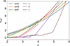 |
Fig. 1. Effective opacity (averaged over an ensemble of lines of sight) due to neutral hydrogen gas in the IGM as a function of redshift, for different wavelengths corresponding to the six Swift-UVOT filters. Solid lines show the results obtained from the analytical model of Inoue et al. (2014b). Dashed lines indicate the results adopted from Fig. 3 of Ghisellini et al. (2010), overplotted for comparison. |
3.3. Fitting procedure
Our goal was to derive the posterior probability density p from Bayes’ theorem given a data set (D) and priors for a model with parameters contained in the vector ϑ (Gregory 2005; Hogg et al. 2010). The likelihood function reads
![Mathematical equation: $$ \begin{aligned} \ln {\mathcal{L} ({\vartheta }|D)} = -\frac{1}{2} \sum _{i}^ \left[\frac{(\phi _{\rm m,i}-\phi _{\rm d, i})^2}{\sigma _{\rm tot, i}^2} + \ln {\sigma _{\rm tot, i}^2} \right], \end{aligned} $$](/articles/aa/full_html/2026/04/aa57154-25/aa57154-25-eq10.gif) (4)
(4)
where i runs over the number of observations, ϕ ≡ log10(νFν), and the subscripts m and d refer to the model expectation and the data, respectively. The comparison of the model and the data was performed in the rest frame of the blazar2, and σtot is defined as
 (5)
(5)
Here, σi is the statistical uncertainty of the flux measurement i (in logarithmic units). We also introduced the term lnf to account for other sources of uncertainty that are not captured by σi. For example, scatter in the photometric data may arise from long-term variability of the disk and/or jet. In addition, photometric fluxes represent averages over the filter bandwidth, while model fluxes are evaluated at a single frequency that corresponds to the central wavelength of the filter. In addition, the use of the term lnf avoids pathological cases in which no statistical errors are reported for the archival photometric data.
We also included upper limits on fluxes in the fit by adding the following term to the likelihood function (see Sawicki 2012; Yang et al. 2020):
![Mathematical equation: $$ \begin{aligned} \sum _j^ \ln \left( \sqrt{\frac{\pi }{2}}\sigma _{\rm j} \left[1+\text{ erf}\left(\frac{\phi _{\rm lim,j}-\phi _{\rm m,j}}{\sqrt{2} \sigma _{\rm j}}\right) \right] \right), \end{aligned} $$](/articles/aa/full_html/2026/04/aa57154-25/aa57154-25-eq12.gif) (6)
(6)
where ϕlim, j is the j-th logarithmic flux upper limit and σj is the uncertainty. Finally, the parameters vector for the two-component model is ϑ = {MBH,Ṁ.F0, s, νc, ln f}, which reduces to {MBH,Ṁ, ln f} for the single accretion disk model.
To estimate the physical parameters of the accretion disk, we performed Markov chain Monte Carlo (MCMC) sampling using the emcee algorithm (Foreman-Mackey et al. 2013). We used uniform priors in logarithmic space for all parameters except the power-law slope, which was uniform in linear space. The mass accretion rate was limited to the Eddington value, since the adopted disk model is not appropriate for describing super-Eddington accretion (see Table 2 for the adopted ranges). We used 20 walkers, 10 000 (5000) steps for the two- (one-)component models, and discarded an appropriate number of points (typically 500–1000) during the burn-in phase3. This ensured that we only retained walkers from the converged solution.
Uniform priors used in the MCMC fit.
4. Results
Tables B.1 and B.2 present the results of the MCMC fitting. More than half of the sample (16 of the 23 sources) was fit with a two-component (jet plus disk) model. The black hole masses lie in the range 3 × 10⁸ M⊙ − 1010 M⊙, and the inferred mass accretion rates are 2 M⊙/yr ≲ M⊙ ≲ 200 M⊙/yr. We find no strong correlation between the black hole mass and mass accretion rates. However, we find an empirical relation between the two variables, taking into account the likely scatter introduced by the unknown black hole spin (for more details, see Appendix D).
We present representative results of our MCMC fit to the photometric SEDs of three high-z blazars from the sample4. Figs. 2 and 4 show the SEDs and reduced corner plots, respectively. A decomposition of the jet plus disk SED model is also shown in Fig. 3. Inspection of the corner plots reveals that fits neglecting extinction from hydrogen gas in the IGM lead to an overestimation of the black hole masses and an underestimation of the Eddington ratios; this effect generally increases with redshift. The effects of extinction on parameter estimation across the sample are presented in Appendix C.
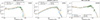 |
Fig. 2. Infrared-to-ultraviolet SEDs of three high-z blazars (in the observer frame). Green points indicate publicly available photometric observations from the ASI SSDC SED builder (Stratta et al. 2011). Upper limits are plotted with black arrows. Model fits with and without IGM extinction are plotted with blue and orange colors, respectively. Dark shaded regions indicate the 68 percent confidence intervals. Thin solid lines indicate the range of model expectations accounting for the intrinsic scatter described by the parameter lnf. All sources, except for J064632+445116, are fit with a two-component (jet plus disk) model. |
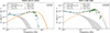 |
Fig. 3. Decomposition of the total (jet plus disk) model SEDs presented in Fig. 2. For clarity, individual spectral components are plotted without IGM attenuation, with the power law in gray and the multi-temperature blackbody in orange. |
 |
Fig. 4. Reduced corner plots for four blazars, showing posterior distributions of MBH, Ṁ, and lnf. The Eddington ratio distribution (derived quantity) is also shown for comparison. Colors are the same as in Fig. 2. |
We selected the three objects to highlight the distinct capabilities of the MCMC SED fitting procedure. SDSS J0131–0321 is included as a high-redshift case to demonstrate the performance of the method under strong IGM attenuation and to verify recovery of the disk peak at large cosmological distances. J064632+445116 exemplifies the case where a single spectral component can describe the data. Its SED includes high-frequency upper limits, showcasing the likelihood treatment of censored data, and illustrating how upper limits influence the posterior without biasing mass inference. Finally, we selected PKS 2149–306 as a well-sampled source at lower redshifts. It has dense multi-wavelength coverage and satisfactorily converged MCMC chains (particularly when IGM extinction is accounted for), providing a prototypical comparison for both complex and data-limited fits.
Figure 5 presents a compact four-panel comparison between our MCMC-derived estimates (including extinction) and the literature values for the black hole mass MBH (left column) and the Eddington ratio λEdd (right column). The error bars indicate the 68% confidence interval of the posterior distributions. The uncertainties in the Eddington ratio are typically larger than those in the black hole mass, as they also incorporate the uncertainty in the estimation of the mass accretion rate. All literature values, except three measurements obtained with spectroscopic methods (see Table 1), lack reported uncertainties.
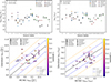 |
Fig. 5. Comparison between our MCMC estimates (including extinction) and literature values for black hole mass MBH (left column) and Eddington ratio λEdd (right column). Top left panel: Black hole mass estimates for each source (x axis index) from our MCMC (black circles) and literature (colored markers; open symbols for spectroscopic and filled for SED-fitting estimates). Error bars show 68% uncertainties. Marker shapes indicate different literature sources. Top right panel: Eddington ratio comparison, using the same visual coding as the left panel. Bottom left panel: Direct comparison of black hole mass estimates between our MCMC method (x axis) and literature values (y axis). Points are colored by source redshift z, and marker shapes indicate literature sources. Open symbols represent spectroscopic measurements, while filled symbols denote SED-fitting estimates. We show the MCMC uncertainties (68% confidence). Bottom right panel: Eddington ratio comparison using the same format, redshift coloring, and marker coding system. In the bottom panels, lines are overplotted to guide the eye (see inset legend). Blazars B2 1023+25 and GB6 B1428+4217 are not shown for reasons explained in Appendix B. Upward-pointing arrows indicate lower limits on the MCMC Eddington ratio estimates for the sources marked in B.1. |
The top row presents source-by-source comparisons, with each object positioned at its original index on the x axis. Points are grouped by literature source (each reference is represented by a distinct marker shape and color) to test for paper-specific systematics. Visual inspection of the top panels reveals no evidence of systematic offsets associated with particular studies, as points from each reference are distributed around our MCMC values without consistent clustering. Approximately half of the sample exhibits black hole mass estimates from the literature that exceed our MCMC results, with discrepancies reaching up to a factor of five in some cases. Notably, for sources where both spectroscopic and SED-based mass estimates are available in the literature, our MCMC results typically align more closely with the spectroscopic measurements. The bottom row uses identical marker shapes for a given literature group, but maps the marker color to the redshift. Trends with marker color could reveal biases that increase with redshift (such as stronger IGM attenuation, reduced photometric coverage of the disk peak, or calibration differences between optical and IR surveys that dominate at different redshifts). We find no indication of redshift-dependent trends in either black hole mass or the Eddington ratio. Interestingly, we find blazars accreting at high Eddington ratios, λEdd > 0.4, both at z ∼ 2 − 3 and z ∼ 5 − 6.
5. Discussion
In our analysis, we hypothesized that the accretion disk extends down to six gravitational radii from the black hole, which is equivalent to assuming non-spinning black holes in all sources. Sect. 5.1 discusses how a nonzero black hole spin would affect our results. Moreover, in Sect. 5.2, we discuss the implications of our results for the black hole seeds of high-z blazars within the framework of Eddington-limited black hole growth.
5.1. Effect of black hole spin on the thin-disk spectrum
For this discussion, we adopt the standard multi-temperature blackbody prescription with a zero-torque inner boundary and the inner disk edge located at the innermost stable circular orbit (ISCO), which depends on the dimensionless Kerr spin parameter a (Shakura & Sunyaev 1973; Bardeen et al. 1972; Novikov & Thorne 1973). For a Kerr black hole, the ISCO radius is given by
 (7)
(7)
![Mathematical equation: $$ \begin{aligned} Z_1(a)&= 1 + (1 - a^2)^{1/3}\Big [(1+a)^{1/3} + (1-a)^{1/3}\Big ], \end{aligned} $$](/articles/aa/full_html/2026/04/aa57154-25/aa57154-25-eq14.gif) (8)
(8)
 (9)
(9)
The local effective temperature profile also follows Eq. (1), where Rin = RISCO; we do not apply the relativistic correction factors, which are discussed in Novikov & Thorne 1973.
The maximum disk temperature, attained near r ≈ Rin, scales as  . The peak frequency, νpeak, of the accretion disk spectrum in units of νFν is νpeak ∝ Tmax, and the corresponding peak flux scales as (νFνAD)max ∝ Tmax4Rin2. From these scalings, the effect of changing spin can be exactly compensated for if both MBH and Ṁ are adjusted simultaneously.
Let primed and unprimed quantities represent the variables of a black hole with spin a ≠ 0 and a = 0, respectively. Imposing the same observed peak frequency and peak flux, we derive the following relations:
 (10)
(10)
 (11)
(11)
Combining these relations yields the rescaling of the black hole mass and accretion rate:
 (12)
(12)
For example, changing from a = 0 (Rin = 6) to a = 0.998 (Rin ≃ 1.24) yields
 (13)
(13)
in order to keep νpeak and (νFνAD)max unchanged.
To illustrate the impact of black hole spin on our results, we selected the source GB6 0805+614 from the sample, where extinction was minor, and repeated the MCMC fit assuming a maximally spinning black hole. Fig. 6 presents the results. The SEDs are identical to those of a non-spinning black hole, if the black hole is more massive and accretes at a lower rate, in agreement with the scalings of Eq. 13. The Eddington ratio for the solution of a maximally spinning black hole is ≈0.04 times smaller than the Eddington ratio for the non-spinning black hole solution. In this example,  for a = 0.998, where the validity of the adopted radiatively efficient disk model breaks down (e.g., Narayan & Yi 1995).
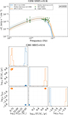 |
Fig. 6. Effects of black hole spin on SED disk-fitting results. Top panel: SED of GB6 0805+614 with MCMC modeling results for a black hole with a = 0.998 and a = 0 overplotted in blue and orange, respectively. Bottom panel: Corner plot of posterior distributions for Ṁ,MBH, and λEdd for both spins (same color coding). Different (MBH,Ṁ) pairs produce identical accretion disk spectra. |
Our current disk model does not include general relativistic effects, which become increasingly important for rapidly spinning black holes. Recently, Hagen & Done (2023) introduced RELAGN, a public code that accounts for both special and general relativistic effects. To explore the impact of relativistic effects, we applied RELAGN to GB6 0805+614. We searched for parameters that produce the same peak flux and position as those of our best-fit SEDs shown in Fig. 6. For α = 0 and 0.998, we find MBH = 4 × 10⁹ M⊙ and 1010 M⊙, with corresponding Eddington ratios of log10λEdd = −1.84 and −1.9, respectively. Therefore, accounting for relativistic effects in disk modeling reduces the discrepancies in the inferred black hole mass and nearly eliminates the dependence of the Eddington ratio on black hole spin.
In summary, black hole spin introduces systematic degeneracy: a disk formed around a high–spin black hole can reproduce the same SED peak frequency and flux as a disk around a low–spin black hole by trading off MBH and Ṁ according to the scalings above. In practice, this means that the estimates of MBH and Ṁ from the SED disk fitting can be biased by up to a factor of five (with the Eddington ratios biased by up to a factor of 25), depending on the assumed spin, unless external constraints are used. For example, the luminosity of the BLR can provide a prior on the disk luminosity through the relation LBLR ≃ (fBLR/0.1) Ldisk, but this approach introduces additional uncertainties associated with the covering fraction and the conversion from line to bolometric luminosity. However, we note that the differences found between the literature values and the MCMC fit results of this work (shown in Fig. 5) cannot be attributed to the black hole spin, as these studies also assumed zero-spin black holes.
5.2. Black hole seed masses
To derive strict lower bounds on the seed masses required to assemble the black holes observed in our sample, we used the Eddington-limited black hole growth solution for radiatively efficient accretion.
Let M(t) denote the black hole mass at cosmic time t5, η the radiative efficiency of the disk, and λ ≡ λEdd the Eddington ratio. The mass growth rate is
 (14)
(14)
and, using LEdd = (4πGmpc/σT)M, we obtain
 (15)
(15)
Here τS is the Salpeter time (Salpeter 1964), the characteristic e-folding scale for Eddington-limited growth. Assuming constant η and λ, the integration yields
![Mathematical equation: $$ \begin{aligned} M(t)=M_{\rm seed}\exp \!\left[\frac{\lambda (1-\eta )}{\tau _S}(t-t_0)\right], \end{aligned} $$](/articles/aa/full_html/2026/04/aa57154-25/aa57154-25-eq24.gif) (16)
(16)
which can be inverted to give the seed mass at formation time t0 required to reach Mfinal ≡ M(tobs) by observation time tobs,
![Mathematical equation: $$ \begin{aligned} M_{\rm seed}=M_{\rm final}\exp \!\left[-\frac{\lambda (1-\eta )}{\tau _S}(t_{\rm obs}-t_0)\right]. \end{aligned} $$](/articles/aa/full_html/2026/04/aa57154-25/aa57154-25-eq25.gif) (17)
(17)
Equation (17) thus returns the mathematically minimal seed mass consistent with constant radiative efficiency, uninterrupted accretion at fixed λ, no black hole mergers, and no extended super-Eddington phases. If accretion is intermittent, λ should be replaced by λeff = fdutyλ, where fduty is the accretion duty cycle (the fraction of cosmic time during which the black hole accretes at the assumed Eddington ratio). Values of fduty < 1, or the inclusion of mergers, episodic super-Eddington phases, or evolving spin-dependent efficiencies, would relax the strict lower bounds derived here (Volonteri 2010; Valiante et al. 2016; Inayoshi et al. 2020).
Table 3 presents the inversion results for 21 blazars from our sample. We adopted the median values for Mfinal and for the Eddington ratio λEdd from the MCMC fits of this work, assumed seed formation at zseed = 20 (cosmic time t0), and fixed η = 0.1. The table reports the observed redshift zobs, λEdd, Mfinal, the available growth interval (tobs − t0), the inferred seed mass, and a classification according to the seeding channel. We adopted the following literature-motivated bands: “very light seeds”, Mseed < 1 M⊙; Pop III remnants (light seeds), 1−103 M⊙ (Volonteri 2010; Inayoshi et al. 2020); stellar-dynamical or cluster-runaway seeds, 103−104 M⊙ (Inayoshi et al. 2020); direct-collapse black holes (DCBHs), 104−106 M⊙(Valiante et al. 2016; Inayoshi et al. 2020); and “very massive seeds”, Mseed ≥ 106 M⊙. In particular, the label very light seed was introduced to flag formal minima below one solar mass, which are not physical (they cannot arise from stellar evolution), and therefore demand cautious interpretation. As a visual complement to Table 3, Fig. 7 shows the reconstructed growth tracks of representative objects compared to the expected seed formation channels.
 |
Fig. 7. Black hole growth histories for the investigated objects. The shaded horizontal regions correspond to different black hole seeding channels: Pop III remnants (Mseed ≲ 102 M⊙; gray), stellar dynamical processes (Mseed ∼ 103 − 104 M⊙; cyan), and direct collapse (Mseed ∼ 104 − 106 M⊙; orange). These seed mass ranges follow the classification described in Valiante et al. (2016). Parts of tracks with Mseed < 1 M⊙ are shown in light gray, as such low masses are not expected to form black holes. |
Inferred seed masses Mseed for our blazar sample.
The formally tiny values of Mseed reported in Table 3 should be regarded as nonphysical minima that signal a degeneracy in the sample and the uninterrupted Eddington-limited growth assumption embodied in Eq. 17. Three interpretations can resolve the unphysically low seed mass: (i) the seeds formed at a later cosmic epoch z0 (hence the available growth time Δt = tobs−t0 is smaller), (ii) accretion was intermittent, so that the effective growth rate is reduced by a duty cycle fduty < 1, or (iii) the black hole was fast spinning, thus the Eddington rate is lower than the values obtained in this work (as discussed in 5.1).
To quantify the second possibility, we replaced the fit Eddington ratio λ by an effective value λeff = fdutyλ. Rearranging Eq. (17) for fduty and imposing Mseed = 10 M⊙ gives
where we adopted η = 0.1 and Δt is the growth interval used in Table 3 (computed assuming seeds form at z0 = 20).
Table 4 shows that, under the conservative assumptions stated above, these seven objects require duty cycles of 0.5-0.7 if their seeds had masses of 10 M⊙ and formed at z0 = 20. Alternatively, if accretion proceeded continuously (fduty = 1), the formation redshifts required for a seed 10 M⊙ span a wide range. Some sources would be consistent with seeds forming at relatively modest redshifts (z0 ∼ 4.0 for PKS 0528+134), while others, such as SDSS J142048.01+120545.9, would require seed formation at high redshifts (z0 > 6).
Duty cycles of blazars.
Several important caveats apply. First, the radiative efficiency η enters linearly into the Salpeter time, and therefore higher values of η increase the required duty cycle or formation redshift. As a result, uncertainties in black hole spin and accretion geometry propagate directly into these inferences (Volonteri 2010). Second, mergers and short episodes of super-Eddington accretion (both plausible in galaxy formation) reduce the need for long, continuous Eddington-limited accretion and would significantly relax the constraints in Table 4 (Begelman et al. 2006; Volonteri 2010). Additional support for this interpretation comes from the semi-analytic and merger-driven calculations of Yoo & Miralda-Escudé (2004), who demonstrated that when hierarchical mergers are included alongside sustained Eddington-limited gas accretion, stellar-remnant seeds with masses of order Mseed ∼ 10 M⊙ can plausibly grow to ∼ 109 M⊙ by z ≃ 6.4. This provides a concrete example in which the very light seed entries in Table 4 can be reconciled with physically plausible seed masses through the inclusion of mergers and prolonged accretion. Therefore, the label very “light seed – unphysical” in Table 3 should be interpreted as a flag that the inversion is exposing a degeneracy between formation epoch and duty cycle, rather than implying literal sub-stellar black holes.
For the objects labeled very massive seed in Table 3, the inverted minima obtained under our assumptions formally require birth masses ≳ 106 M⊙. This result does not force a unique interpretation. Hierarchical mergers of smaller remnants, coupled with sustained near-Eddington accretion, can assemble very large black holes within the available cosmic time (Yoo & Miralda-Escudé 2004; Volonteri 2010; Valiante et al. 2016). Alternatively, super-Eddington (super-critical) accretion episodes, demonstrated in semi-analytic work and multidimensional simulations (cosmological semi-analytic models, 3D hydrodynamical circumnuclear simulations, and global 3D radiation and magneto-hydrodynamic accretion-flow calculations) can accelerate growth relative to strict Eddington-limited evolution, providing an alternative pathway for stellar-mass seeds to reach high masses rapidly (Lupi et al. 2016; Pezzulli et al. 2016; Sądowski & Narayan 2016; Inayoshi et al. 2020).
Table 3 shows that sources with the lowest Eddington ratios (0.04 ≤ λ < 0.3) require very massive seeds, while sources with higher Eddington ratios (λ > 0.4) require very light seeds. This pattern arises from the exponential growth law of Eq. (17), assuming constant radiative efficiency. Consequently, uncertainties in the Eddington ratio can strongly affect the inferred seed masses.
This is also exemplified in the specific case of PSO J0309+27, which Belladitta et al. (2022) study in detail. Using our updated values for PSO J0309+27 from Table 3, and replacing the Eddington ratio with λ = 0.44, as reported by Belladitta et al. (2022), reduces the required seed mass by a factor of approximately 50. Our formal estimate of Mseed ≃ 1.8 × 10⁸ M⊙ (based on λ = 0.16) would decrease to ∼3.8 × 10⁶ M⊙ when adopting their higher Eddington ratio. If we also adopt their final mass estimate (Mfinal ≃ 1.45 × 10⁹ M⊙) and their assumed seed formation redshift (z0 = 30), the inferred initial mass decreases further to ∼1.1 × 10⁶ M⊙ under η = 0.1. The difference in the adopted Eddington ratio and formation redshift largely explains the apparent discrepancy between our seed scenario for PSO J0309+27 and that discussed by Belladitta et al. (2022).
6. Conclusions
We have presented a homogeneous analysis of 23 high-redshift blazars spanning from z ∼ 2 to z ∼ 6 using archival infrared-to-ultraviolet photometric data and a Bayesian MCMC fitting of the Shakura–Sunyaev accretion disk model. By including the effects of IGM attenuation, we derive black hole masses and mass accretion rates with quantified uncertainties and avoid the systematic overestimation of MBH (up to a factor of 11) that arises when extinction is neglected. Our results show no evidence for systematic offsets relative to previous literature values, while we recover accretion rates ranging from ∼0.05 to ∼0.99 across the sample. We find no evidence of correlation between the black hole masses and Eddington ratios with redshift. We further examined the potential impact of black hole spin, showing how it can influence the derived accretion-disk parameters. Using the Eddington-limited growth equation, we placed lower limits on the seed masses required to assemble the observed black holes. The results highlight a broad range of possible seeding channels, from Pop III to direct-collapse black holes, with the required seed mass strongly correlated with the used Eddington ratio.
To our knowledge, this is the first systematic study to model thermal disk emission from a large sample of high-z blazars within a common statistical framework. By providing the largest uniform set of black hole mass and accretion-rate estimates for these sources with accompanying uncertainties, our results underscore the importance of consistent modeling when comparing across diverse samples. Future progress will rely on improved multiwavelength coverage of the disk emission, as well as independent constraints on spin and accretion histories, which are essential to resolve the degeneracies inherent in SED-based mass determinations.
Data availability
Archival data, MCMC fitting results (in .h5 format), and Python scripts to plot results for individual sources are available for download at this link: https://zenodo.org/records/17781963.
Acknowledgments
The authors thank the anonymous referee for their constructive comments that help to improve the manuscript. The authors also thank Andrea Gokus for bringing to their attention another high-z blazar that was added to the analysis. The authors thank Lea Marcotulli for providing the photometric data presented in Marcotulli et al. (2020) and John Kallimanis for useful discussions about statistical methods. M.P. acknowledges support from the Hellenic Foundation for Research and Innovation (H.F.R.I.) under the “2nd call for H.F.R.I. Research Projects to support Faculty members and Researchers” through the project UNTRAPHOB (Project ID 3013). G.V. acknowledges support from the H.F.R.I. through the project ASTRAPE (Project ID 7802).
References
- Ackermann, M., Ajello, M., Baldini, L., et al. 2017, ApJ, 837, L5 [CrossRef] [Google Scholar]
- Bardeen, J. M., Press, W. H., & Teukolsky, S. A. 1972, ApJ, 178, 347 [Google Scholar]
- Begelman, M. C., Volonteri, M., & Rees, M. J. 2006, MNRAS, 370, 289 [NASA ADS] [CrossRef] [Google Scholar]
- Belladitta, S., Caccianiga, A., Diana, A., et al. 2022, A&A, 660, A74 [NASA ADS] [CrossRef] [EDP Sciences] [Google Scholar]
- Burrows, D. N., Hill, J. E., Nousek, J. A., et al. 2005, Space Sci. Rev., 120, 165 [Google Scholar]
- Calderone, G., Ghisellini, G., Colpi, M., & Dotti, M. 2013, MNRAS, 431, 210 [NASA ADS] [CrossRef] [Google Scholar]
- Cardelli, J. A., Clayton, G. C., & Mathis, J. S. 1989, ApJ, 345, 245 [Google Scholar]
- Diana, A., Caccianiga, A., Ighina, L., et al. 2022, MNRAS, 511, 5436 [NASA ADS] [CrossRef] [Google Scholar]
- Dietrich, M., & Hamann, F. 2004, ApJ, 611, 761 [NASA ADS] [CrossRef] [Google Scholar]
- Foreman-Mackey, D., Hogg, D. W., Lang, D., & Goodman, J. 2013, PASP, 125, 306 [Google Scholar]
- Frank, J., King, A., & Raine, D. J. 2002, Accretion Power in Astrophysics: Third Edition (Cambridge, UK: Cambridge University Press) [Google Scholar]
- Ghisellini, G. 2016, Galaxies, 4, 36 [Google Scholar]
- Ghisellini, G., Della Ceca, R., Volonteri, M., et al. 2010, MNRAS, 405, 387 [NASA ADS] [Google Scholar]
- Ghisellini, G., Tagliaferri, G., Foschini, L., et al. 2011, MNRAS, 411, 901 [Google Scholar]
- Ghisellini, G., Nardini, M., Tagliaferri, G. J., et al. 2013, MNRAS, 428, 1449 [Google Scholar]
- Ghisellini, G., Tavecchio, F., Maraschi, L., Celotti, A., & Sbarrato, T. 2014, Nature, 515, 376 [NASA ADS] [CrossRef] [Google Scholar]
- Ghisellini, G., Tagliaferri, G., Sbarrato, T., & Gehrels, N. 2015, MNRAS, 450, L34 [NASA ADS] [CrossRef] [Google Scholar]
- Giommi, P., Padovani, P., Polenta, G., et al. 2012a, MNRAS, 420, 2899 [NASA ADS] [CrossRef] [Google Scholar]
- Giommi, P., Polenta, G., Lähteenmäki, A., et al. 2012b, A&A, 541, A160 [NASA ADS] [CrossRef] [EDP Sciences] [Google Scholar]
- Gokus, A., Böttcher, M., Errando, M., et al. 2024, ApJ, 974, 38 [Google Scholar]
- Gokus, A., Errando, M., Agudo, I., et al. 2025, ApJ, 990, 206 [Google Scholar]
- Gregory, P. C. 2005, Bayesian Logical Data Analysis for the Physical Sciences: A Comparative Approach with ‘Mathematica’ Support (Cambridge, UK: Cambridge University Press) [Google Scholar]
- Greiner, J., Bornemann, W., Clemens, C., et al. 2008, PASP, 120, 405 [Google Scholar]
- Gunn, J. E., & Peterson, B. A. 1965, ApJ, 142, 1633 [Google Scholar]
- Haakonsen, C. B., & Rutledge, R. E. 2009, ApJS, 184, 138 [NASA ADS] [CrossRef] [Google Scholar]
- Haardt, F., & Madau, P. 2012, ApJ, 746, 125 [Google Scholar]
- Hagen, S., & Done, C. 2023, MNRAS, 525, 3455 [NASA ADS] [CrossRef] [Google Scholar]
- HI4PI Collaboration (Ben Bekhti, N., et al.) 2016, A&A, 594, A116 [NASA ADS] [CrossRef] [EDP Sciences] [Google Scholar]
- Hogg, D. W. 2000, arXiv e-prints [arXiv:astro-ph/9905116] [Google Scholar]
- Hogg, D. W., Bovy, J., & Lang, D. 2010, arXiv e-prints [arXiv:1008.4686] [Google Scholar]
- Hovatta, T., & Lindfors, E. 2019, New Astron. Rev., 87, 101541 [CrossRef] [Google Scholar]
- Inayoshi, K., Visbal, E., & Haiman, Z. 2020, ARA&A, 58, 27 [NASA ADS] [CrossRef] [Google Scholar]
- Inoue, A. K., Shimizu, I., & Iwata, I. 2014a, Astrophysics Source Code Library [record ascl:1402.019] [Google Scholar]
- Inoue, A. K., Shimizu, I., Iwata, I., & Tanaka, M. 2014b, MNRAS, 442, 1805 [NASA ADS] [CrossRef] [Google Scholar]
- Jarrett, T. H., Cohen, M., Masci, F., et al. 2011, ApJ, 735, 112 [Google Scholar]
- Kaspi, S., Smith, P. S., Netzer, H., et al. 2000, ApJ, 533, 631 [Google Scholar]
- Lupi, A., Haardt, F., Dotti, M., et al. 2016, MNRAS, 456, 2993 [NASA ADS] [CrossRef] [Google Scholar]
- Marcotulli, L., Paliya, V., Ajello, M., et al. 2020, ApJ, 889, 164 [NASA ADS] [CrossRef] [Google Scholar]
- Narayan, R., & Yi, I. 1995, ApJ, 452, 710 [NASA ADS] [CrossRef] [Google Scholar]
- Novikov, I. D., & Thorne, K. S. 1973, in Black Holes (Les Astres Occlus), eds. C. Dewitt, & B. S. Dewitt, 343 [Google Scholar]
- Pezzulli, E., Valiante, R., & Schneider, R. 2016, MNRAS, 458, 3047 [NASA ADS] [CrossRef] [Google Scholar]
- Planck Collaboration XIII. 2016, A&A, 594, A13 [NASA ADS] [CrossRef] [EDP Sciences] [Google Scholar]
- Reines, A. E., & Comastri, A. 2016, PASA, 33, e054 [Google Scholar]
- Roming, P. W. A., Kennedy, T. E., Mason, K. O., et al. 2005, Space Sci. Rev., 120, 95 [Google Scholar]
- Sądowski, A., & Narayan, R. 2016, MNRAS, 456, 3929 [CrossRef] [Google Scholar]
- Salpeter, E. E. 1964, ApJ, 140, 796 [NASA ADS] [CrossRef] [Google Scholar]
- Sanchez Zaballa, J. M., Bottacini, E., & Tramacere, A. 2025, ApJ, 985, 179 [Google Scholar]
- Sawicki, M. 2012, PASP, 124, 1208 [NASA ADS] [CrossRef] [Google Scholar]
- Sbarrato, T., Tagliaferri, G., Ghisellini, G., et al. 2013, ApJ, 777, 147 [Google Scholar]
- Sbarrato, T., Ghisellini, G., Tagliaferri, G., et al. 2015, MNRAS, 446, 2483 [NASA ADS] [CrossRef] [Google Scholar]
- Sbarrato, T., Ajello, M., Buson, S., et al. 2025, Space Sci. Rev., 221, 62 [Google Scholar]
- Shakura, N. I., & Sunyaev, R. A. 1973, A&A, 24, 337 [NASA ADS] [Google Scholar]
- Shen, Y., Richards, G. T., Strauss, M. A., et al. 2011, ApJS, 194, 45 [Google Scholar]
- Stratta, G., Capalbi, M., Giommi, P., et al. 2011, arXiv e-prints [arXiv:1103.0749] [Google Scholar]
- Valiante, R., Schneider, R., Volonteri, M., & Omukai, K. 2016, https://doi.org/10.5281/zenodo.163515 [Google Scholar]
- Volonteri, M. 2010, A&ARv, 18, 279 [Google Scholar]
- Volonteri, M., Haardt, F., Ghisellini, G., & Della Ceca, R. 2011, MNRAS, 416, 216 [Google Scholar]
- Wright, E. L., Eisenhardt, P. R. M., Mainzer, A. K., et al. 2010, AJ, 140, 1868 [Google Scholar]
- Yang, G., Boquien, M., Buat, V., et al. 2020, MNRAS, 491, 740 [Google Scholar]
- Yi, W.-M., Wang, F., Wu, X.-B., et al. 2014, ApJ, 795, L29 [Google Scholar]
- Yoo, J., & Miralda-Escudé, J. 2004, ApJ, 614, L25 [NASA ADS] [CrossRef] [Google Scholar]
The emitted photon frequency νem is related to the observed one as νem = ν(1 + z), and νFν = νemFνem.
For each chain of length N, we also computed the integrated autocorrelation time τ and verified N > (40 − 50)τ, which is generally taken as evidence of convergence.
SEDs and corner plots for all sources are available at this link.
Cosmic time t and redshift z are related by (Hogg 2000; Planck Collaboration XIII 2016):
Appendix A: Representative cases of problematic photometry
To construct the SEDs we obtained data from the SED builder tool using a 3″search radius, since the position of the sources is known with high accuracy and can be seen in Table 1. In several SEDs we identified, after visual inspection, a couple of outlier points, either yielding too high or too low fluxes. In the case of IR data (e.g., AllWISE), this could be related to the particular field and the large point-spread function of the instrument. For optical data, this could be due to problems in the catalogs used by the SED builder tool. We therefore proceeded to visually inspect the fields to search for possible contamination and also cross-checked the catalog information at the seemingly problematic data points.
A problem we identified in multiple sources was related to the catalog of Haakonsen & Rutledge (2009). This catalog lists the coordinates of blazars and photometric values (DSS2) for their optical counterparts, without providing the coordinates or an identification for the counterpart. We discovered that the photometric data are not always taken from the correct counterpart, but in some cases from the brightest source located several arc-seconds away. The upper panel in Fig. A.1 shows the case of PKS 2149−306, where we indicate the wrong counterpart with a magenta circle. The three-band image sequence demonstrates that the catalog counterpart does not coincide with the compact optical/IR source identified as the blazar (indicated with a cross). Therefore, we consider this catalog entry to be a misassociation and excluded the corresponding photometry from the SED fitting.
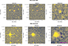 |
Fig. A.1. Two representative examples of problematic photometry identified in SED builder data during our catalog cross-checks and visual inspection. Top: The position of PKS 2149−306 is marked with an open x sign, a catalog cross-match with SED builder tool yields a mix of photometric data from the correct counterpart but also from the nearby bright object marked with a magenta circle, which was misidentified as the optical counterpart in the Haakonsen & Rutledge (2009) catalog. Bottom: Same plot for PKS 0519+01. Contamination from a nearby source is visible in the WISE band when large-aperture photometry is used. The SED builder tool by default returns fluxes from three different extraction methods without a clear distinction. In both examples as well as in all cases with similar issues, the problematic photometric measurements were excluded from the SEDs used in the analysis. |
The lower panel in Fig. A.1 shows the case of PKS 0519+01, where the fixed-radius 22″ aperture provided in the AllWISE catalog (Jarrett et al. 2011) is overplotted as a magenta circle. It is evident that the large fixed aperture encloses flux from a nearby source, producing a biased (overestimated) flux for the blazar when this aperture magnitude is adopted without visual verification. The largest fixed apertures (e.g., the 22″ aperture in W3) are susceptible to contamination in crowded fields and for point sources close to neighbors.
Sources with outlier points.
Appendix B: MCMC fitting results
In this section, we provide the tables B.1 and B.2 with the MCMC fit results for the sources in our sample. To quantitatively compare the SED fits with and without intergalactic medium (IGM) attenuation, we computed the Bayesian Information Criterion (BIC). The resulting BIC values are reported in Table B.1 and provide a measure of the relative goodness of fit while accounting for model complexity. The attenuation implemented in the model is determined by the source redshift and is kept fixed, hence it does not introduce additional free parameters. Although the unattenuated model occasionally yields lower BIC values, this difference likely reflects statistical fluctuations rather than a genuinely better physical description. Because attenuation in high-redshift blazars is expected to occur, and our model employs an average effective H I opacity (not adjusted for individual lines of sight), the BIC alone cannot serve as a decisive criterion for model preference. For this reason, the extinction-corrected fits are adopted throughout our figures and analysis, as they offer a physically consistent representation of the source SEDs.
Fit model parameters from MCMC analysis.
An illustrative example of this limitation is provided by the source B2 1023+25. We were unable to obtain a reliable disk+jet SED fit with attenuation for this object. Inspection of its SED shows that the highest-frequency data points lie systematically above the extinction-corrected model used in our fits (see the supplementary material at the project’s repository). Reproducing those points would require a lower optical depth to H I than the effective value we used. Therefore, the true black hole mass and accretion rate values should lie between those obtained with and without extinction (a similar argument can be made also for GB6 B1428+4217).
Another noteworthy case is that of GB6 B1428+4217. Gokus et al. (2025) analyzed optical data (in the I and R bands) from this blazar during its 2023–2024 flare and reported a polarization degree (8.6±0.3)% in the R band. Such a polarization level indicates a significant contribution from the jet to the observed flux, since the thermal emission from the accretion disk is expected to be largely unpolarized (< 3%). In our analysis, we modeled archival data with a pure accretion disk component; however, part of the R-band flux could plausibly originate from a jet component with an as yet unknown polarization. The disk contribution to the observed R- and I-band fluxes can be reduced below the measured values if a black hole mass about ten times larger and an accretion rate roughly three times lower are assumed. This represents an extreme configuration, adopted here only to illustrate the minimal possible contribution of the disk to the total optical emission. At the same time, the available low-frequency data points (ν ≲ 1014 Hz) are sparse, making it difficult to constrain the jet component directly. This limitation likely explains why a single-component (disk-only) model is statistically preferred in our fits. In such cases, broadband SED modeling of the jet emission, as performed by Gokus et al. (2025), may provide the most reliable means to constrain the disk properties.
 |
Fig. B.1. Ratios of quantities derived with and without accounting for extinction. The top row shows the ratio of black hole masses (left) and the ratio of accretion rates (right), while the bottom panel shows the ratio of Eddington ratios. The dashed black vertical line at R = 1 corresponds to no change between the two fits. These plots highlight the systematic trend: neglecting extinction leads to overestimates of black hole masses and underestimates of Eddington ratios. The blazars B2 1023+25 and GB6 B1428+4217 are excluded from this figure because of reasons explained in Appendix B. |
Best-fit parameters of the power-law component (with and without extinction) of the jet+disk model.
Appendix C: Impact of extinction on derived quantities
In this section, we quantify how the inclusion of IGM attenuation affects the disk-derived parameters by directly comparing posterior medians obtained with and without absorption. The comparison shown in Fig. B.1 demonstrates how neglecting this effect leads to systematically higher black hole masses and lower Eddington ratios. These results highlight that IGM attenuation must be accounted for in order to obtain more reliable and accurate estimates of the derived quantities.
Appendix D: Black hole mass - accretion rate: Empirical modeling with spin-induced covariance
We model the relationship between black hole mass MBH, and accretion rate Ṁ, in logarithmic space using a linear relation
 (D.1)
(D.1)
where m is the slope and b the offset. The masses and accretion rates used in the fit were taken from our spectral MCMC runs performed under the assumption of non-rotating black holes (a = 0). Because the true spins are unknown, this induces a systematic degeneracy between the inferred black hole mass MBH and the accretion rate Ṁ via the spin-dependent inner radius RISCO(a) (Eq. 12). This spin-induced uncertainty produces an additive shift δ = log10(Rin, ref/Rin) in log10MBH and −δ in log10 Ṁ, introducing a covariance along the y = −x direction.
This effect can be represented as a covariance matrix per-object in logarithmic space,
 (D.2)
(D.2)
which is added to the measurement covariance, effectively capturing the scatter induced by the spin distribution. The total residual perpendicular to the linear relation, d⊥, is assumed to be Gaussian distributed. The corresponding log-likelihood is then
![Mathematical equation: $$ \begin{aligned} \ln \mathcal{L} = \sum _i -\frac{1}{2} \left[ \ln \left(2\pi \, \sigma _{\perp ,i}^2 \right) + \frac{d_{\perp ,i}^2}{\sigma _{\perp ,i}^2} \right], \end{aligned} $$](/articles/aa/full_html/2026/04/aa57154-25/aa57154-25-eq260.gif) (D.3)
(D.3)
where σ⊥, i2 = nT(Σmeas, i + Σδ, i)n + σ⊥2, n is the unit normal vector to the line, and σ⊥ accounts for additional intrinsic scatter.
To account for measurement errors, each source is represented by a “cloud” of K realizations in logarithmic space:

where xi= log10 Ṁi (with Ṁ in M⊙ yr−1) and yi = log10MBH,i (with MBH expressed in units of 109 M⊙). For each draw, we sample a spin ai,j ∼ 𝒰[0,1), compute RISCO(ai,j) from Eq. 7, rescale the linear-space pair {MBH,Ṁ} according to Eq. 12 with reference radius Rref = 6 Rg, and then map the rescaled values back to (xi,j,yi,j).
Finally, we sample the posterior distribution of (m, b, σ⊥) using UltraNest, marginalizing over both spin-induced uncertainty and measurement errors. The resulting posterior provides the best-fit linear relation and associated credible intervals. In Fig. D.1 we plot the fit MBH and Ṁ values with their errors, together with the clouds of realizations based on the spin distributions. We also indicate the direction of the spin-induced scatter with an arrow. The best-fit linear model is shown with a gray shaded area and solid line, while the dashed red lines represent the fit scatter.
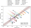 |
Fig. D.1. Log-log plot of MBH and Ṁ plot based on our fit results assuming zero BH spin (black points indicate the median values from the posterior distributions). Colored clouds are computed based on statistical uncertainties of the fit, as well as a correction for uniform spin following Eq. D.2 that causes a scatter in the direction of the arrow (see text for details). The population is fit by a linear model defined in Eq. D.1. The median and the 68% credible region are marked by the gray line and the shaded region respectively. Red lines mark the median excess scatter predicted by the fit due to BH spin uncertainty. |
All Tables
Best-fit parameters of the power-law component (with and without extinction) of the jet+disk model.
All Figures
|
Fig. 1. Effective opacity (averaged over an ensemble of lines of sight) due to neutral hydrogen gas in the IGM as a function of redshift, for different wavelengths corresponding to the six Swift-UVOT filters. Solid lines show the results obtained from the analytical model of Inoue et al. (2014b). Dashed lines indicate the results adopted from Fig. 3 of Ghisellini et al. (2010), overplotted for comparison. |
| In the text | |
|
Fig. 2. Infrared-to-ultraviolet SEDs of three high-z blazars (in the observer frame). Green points indicate publicly available photometric observations from the ASI SSDC SED builder (Stratta et al. 2011). Upper limits are plotted with black arrows. Model fits with and without IGM extinction are plotted with blue and orange colors, respectively. Dark shaded regions indicate the 68 percent confidence intervals. Thin solid lines indicate the range of model expectations accounting for the intrinsic scatter described by the parameter lnf. All sources, except for J064632+445116, are fit with a two-component (jet plus disk) model. |
| In the text | |
|
Fig. 3. Decomposition of the total (jet plus disk) model SEDs presented in Fig. 2. For clarity, individual spectral components are plotted without IGM attenuation, with the power law in gray and the multi-temperature blackbody in orange. |
| In the text | |
|
Fig. 4. Reduced corner plots for four blazars, showing posterior distributions of MBH, Ṁ, and lnf. The Eddington ratio distribution (derived quantity) is also shown for comparison. Colors are the same as in Fig. 2. |
| In the text | |
|
Fig. 5. Comparison between our MCMC estimates (including extinction) and literature values for black hole mass MBH (left column) and Eddington ratio λEdd (right column). Top left panel: Black hole mass estimates for each source (x axis index) from our MCMC (black circles) and literature (colored markers; open symbols for spectroscopic and filled for SED-fitting estimates). Error bars show 68% uncertainties. Marker shapes indicate different literature sources. Top right panel: Eddington ratio comparison, using the same visual coding as the left panel. Bottom left panel: Direct comparison of black hole mass estimates between our MCMC method (x axis) and literature values (y axis). Points are colored by source redshift z, and marker shapes indicate literature sources. Open symbols represent spectroscopic measurements, while filled symbols denote SED-fitting estimates. We show the MCMC uncertainties (68% confidence). Bottom right panel: Eddington ratio comparison using the same format, redshift coloring, and marker coding system. In the bottom panels, lines are overplotted to guide the eye (see inset legend). Blazars B2 1023+25 and GB6 B1428+4217 are not shown for reasons explained in Appendix B. Upward-pointing arrows indicate lower limits on the MCMC Eddington ratio estimates for the sources marked in B.1. |
| In the text | |
|
Fig. 6. Effects of black hole spin on SED disk-fitting results. Top panel: SED of GB6 0805+614 with MCMC modeling results for a black hole with a = 0.998 and a = 0 overplotted in blue and orange, respectively. Bottom panel: Corner plot of posterior distributions for Ṁ,MBH, and λEdd for both spins (same color coding). Different (MBH,Ṁ) pairs produce identical accretion disk spectra. |
| In the text | |
|
Fig. 7. Black hole growth histories for the investigated objects. The shaded horizontal regions correspond to different black hole seeding channels: Pop III remnants (Mseed ≲ 102 M⊙; gray), stellar dynamical processes (Mseed ∼ 103 − 104 M⊙; cyan), and direct collapse (Mseed ∼ 104 − 106 M⊙; orange). These seed mass ranges follow the classification described in Valiante et al. (2016). Parts of tracks with Mseed < 1 M⊙ are shown in light gray, as such low masses are not expected to form black holes. |
| In the text | |
|
Fig. A.1. Two representative examples of problematic photometry identified in SED builder data during our catalog cross-checks and visual inspection. Top: The position of PKS 2149−306 is marked with an open x sign, a catalog cross-match with SED builder tool yields a mix of photometric data from the correct counterpart but also from the nearby bright object marked with a magenta circle, which was misidentified as the optical counterpart in the Haakonsen & Rutledge (2009) catalog. Bottom: Same plot for PKS 0519+01. Contamination from a nearby source is visible in the WISE band when large-aperture photometry is used. The SED builder tool by default returns fluxes from three different extraction methods without a clear distinction. In both examples as well as in all cases with similar issues, the problematic photometric measurements were excluded from the SEDs used in the analysis. |
| In the text | |
|
Fig. B.1. Ratios of quantities derived with and without accounting for extinction. The top row shows the ratio of black hole masses (left) and the ratio of accretion rates (right), while the bottom panel shows the ratio of Eddington ratios. The dashed black vertical line at R = 1 corresponds to no change between the two fits. These plots highlight the systematic trend: neglecting extinction leads to overestimates of black hole masses and underestimates of Eddington ratios. The blazars B2 1023+25 and GB6 B1428+4217 are excluded from this figure because of reasons explained in Appendix B. |
| In the text | |
|
Fig. D.1. Log-log plot of MBH and Ṁ plot based on our fit results assuming zero BH spin (black points indicate the median values from the posterior distributions). Colored clouds are computed based on statistical uncertainties of the fit, as well as a correction for uniform spin following Eq. D.2 that causes a scatter in the direction of the arrow (see text for details). The population is fit by a linear model defined in Eq. D.1. The median and the 68% credible region are marked by the gray line and the shaded region respectively. Red lines mark the median excess scatter predicted by the fit due to BH spin uncertainty. |
| In the text | |
Current usage metrics show cumulative count of Article Views (full-text article views including HTML views, PDF and ePub downloads, according to the available data) and Abstracts Views on Vision4Press platform.
Data correspond to usage on the plateform after 2015. The current usage metrics is available 48-96 hours after online publication and is updated daily on week days.
Initial download of the metrics may take a while.