| Issue |
A&A
Volume 708, April 2026
|
|
|---|---|---|
| Article Number | A200 | |
| Number of page(s) | 17 | |
| Section | Galactic structure, stellar clusters and populations | |
| DOI | https://doi.org/10.1051/0004-6361/202557230 | |
| Published online | 08 April 2026 | |
Seeds to success: Growing heavy black holes in dense star clusters
1
Gran Sasso Science Institute (GSSI),
Viale Francesco Crispi 7,
L’Aquila,
Italy
2
INFN, Laboratori Nazionali del Gran Sasso,
67100
Assergi,
Italy
3
Istituto Nazionale di Astrofisica – Osservatorio Astronomico di Roma,
Via Frascati 33,
00040
Monteporzio Catone,
Italy
4
Universität Heidelberg, Zentrum für Astronomie (ZAH), Institut für Theoretische Astrophysik,
Albert Ueberle Str. 2,
69120
Heidelberg,
Germany
★ Corresponding authors: This email address is being protected from spambots. You need JavaScript enabled to view it.
; This email address is being protected from spambots. You need JavaScript enabled to view it.
Received:
12
September
2025
Accepted:
30
January
2026
Abstract
Context. The observational dearth of black holes (BHs) with masses between ∼100 and 100 000 M⊙ raises questions about the nature of intermediate-mass black holes (IMBHs). The proposed formation channels for IMBHs include runaway stellar collisions and repeated binary BH (BBH) mergers driven by dynamical interactions in stellar clusters, but the formation efficiency of these processes and the associated IMBH occupation fraction are largely unconstrained.
Aims. For this work we studied IMBH formation via both mechanisms in young (YCs), globular (GCs), and nuclear star clusters (NSCs). We carried out a comprehensive investigation of IMBH formation efficiency by exploring the impact of different seeding models and star cluster formation histories.
Methods. We employed a new version of the B-POP population synthesis code, able to model several seeding mechanisms as well as hierarchical BBH mergers.
Results. We quantify the efficiency of IMBH production across different cluster families and demonstrate that stellar collisions are essential for sustaining IMBH formation. Furthermore, a comparison with low-redshift IMBH candidates indicates that, depending on the seeding mechanism, they may play a pivotal role in explaining the presence of IMBHs in local GCs.
Conclusions. Our simulations highlight stellar collisions as the primary IMBH formation channel across a wide range of cluster types. They further suggest that wandering IMBHs may populate Milky Way-like galaxies, and that correlations between cluster and IMBH masses can help distinguish the origins of Galactic GCs.
Key words: black hole physics / stars: black holes / galaxies: star clusters: general
© The Authors 2026
 Open Access article, published by EDP Sciences, under the terms of the Creative Commons Attribution License (https://creativecommons.org/licenses/by/4.0), which permits unrestricted use, distribution, and reproduction in any medium, provided the original work is properly cited.
This article is published in open access under the Subscribe to Open model. This email address is being protected from spambots. You need JavaScript enabled to view it. to support open access publication.
1 Introduction
Black holes (BHs) can be broadly classified into two main categories based on their mass. Stellar-mass BHs lie at the low end of the mass scale, with masses ranging from about 3–5 M⊙ up to roughly 100 M⊙. These BHs form from the collapse of massive stars with initial masses greater than approximately 20 M⊙ (see, e.g., Vink et al. 2001; Woosley et al. 2002; Fryer et al. 2012; Spera et al. 2015; Vink et al. 2021; Ugolini et al. 2025). At the opposite extreme are supermassive BHs (SMBHs), which have typical masses exceeding ∼106 M⊙. SMBHs are commonly found at the centers of galaxies and are believed to grow through complex evolutionary processes, starting from lighter BH seeds that increase in mass via various mechanisms (see, e.g., Volonteri et al. 2021; Izquierdo-Villalba et al. 2023). These seeds, which often represent intermediate states between the two BH mass categories, fall in the mass range between ∼102 and 105 M⊙ and belong to the elusive family of intermediate-mass black holes (IMBHs). IMBHs have been extensively studied through a variety of observational channels, including searches for potential radiative accretion signatures (Maccarone & Servillat 2008; Tremou et al. 2018; Lin et al. 2018; Tiengo et al. 2022), integral field spectroscopy and astrometric measurements of stellar motion (Gebhardt et al. 2005; Noyola et al. 2010; van der Marel & Anderson 2010; Lützgendorf et al. 2013a; Lanzoni et al. 2013; Kamann et al. 2014, 2016; Pechetti et al. 2022; Häberle et al. 2024), millisecond pulsar timing (D’Amico et al. 2002; Colpi et al. 2003; Ferraro et al. 2003; Kızıltan et al. 2017; Perera et al. 2017; Gieles et al. 2018; Bañares-Hernández et al. 2025), and gravitational-wave (GW) detections (Abbott et al. 2020; Abac et al. 2025b). Despite the increasing observational evidence, their existence is often difficult to confirm due to the absence of a definitive observational signature and the possibility that their effects can be mimicked by other astrophysical systems or processes. Investigating IMBH formation in different stellar environments, and its potential smoking guns, is therefore fundamental to understanding the nature of these objects and their possible links to stellar and SMBHs.
One promising route for IMBH formation is through dynamical assembly in a dense star cluster. Within this formation scenario, several mechanisms can play a role in the production and growth of the IMBH. Among them are the formation of a very massive star (VMS) from repeated stellar collisions that either collapses into an IMBH or accretes most of its mass on a stellar BH, repeated mergers among BHs and/or stars, or multiple tidal disruption events on stellar BHs (Miller & Hamilton 2002; Portegies Zwart & McMillan 2002; Giersz et al. 2015; Arca Sedda et al. 2023a; Rizzuto et al. 2023). Repeated stellar collisions may occur in light (≲106 M⊙) and compact (≲0.1–1 pc) star clusters, where core collapse sets in before massive stars evolve in compact objects. In these clusters, the density peak reached at collapse can trigger the onset of collisions among massive stars which can proceed in a runaway fashion, hence the term runaway stellar collisions (Portegies Zwart & McMillan 2002). The resulting VMS can reach a mass of ∼0.1-1% of the cluster’s initial mass, eventually collapsing into an IMBH. Conversely, hierarchical binary BH (BBH) mergers (Miller & Hamilton 2002) can trigger the build-up of an IMBH starting from a stellar BH progenitor or can yield the further growth of a seed formed from stellar collisions. This process is expected to take place preferentially in massive, compact clusters with high escape velocities (≳ a few hundred km/s).
Historically, these two fundamental formation channels have been extensively studied through direct N-body and Monte Carlo simulations (see, e.g., Giersz et al. 2015; Mapelli 2016; Kremer et al. 2020; Di Carlo et al. 2021; Rizzuto et al. 2021; Arca Sedda et al. 2023a; Vergara et al. 2024; Barber & Antonini 2024; González Prieto et al. 2024; Rantala et al. 2024; Vergara et al. 2026). However, the computational costs of the two techniques restrict the cluster parameter space that can be investigated (e.g., cluster structure, metallicity, formation history). An appealing alternative that became quite popular in the last few years is represented by semianalytic codes, which encode simplified recipes to model BH dynamics and significantly reduce the required simulation time (Antonini & Rasio 2016; Arca Sedda & Benacquista 2019; Antonini & Gieles 2020; Arca Sedda et al. 2020b; Mapelli et al. 2021; Arca Sedda et al. 2023b; Kritos et al. 2024; Torniamenti et al. 2024).
For this work, we employed the latest version of the semi-analytic population synthesis code B-POP (Arca Sedda & Benacquista 2019; Arca Sedda et al. 2020b, 2023b) to explore possible relations among different IMBH formation scenarios and the properties of their nursing environments. In Sect. 2 we present the main features of B-POP and the different models we investigated for the seeding and the clusters formation history. In Sect. 3, we briefly overview the efficiency of different IMBH formation and growth mechanisms based on the initial properties of the host clusters. Moreover, we present the results of our simulations, focusing on the emergence of IMBHs at low redshifts and their similarities to potential observed candidates. In Sect. 4 we discuss some interesting implications of our findings for different families of clusters. Finally, in Sect. 5 we summarize our main conclusions.
Main B-POP input parameters along with the assigned value and a short description.
2 Methods
We studied the dynamical formation of IMBHs in star clusters under different seeding prescriptions and cluster formation histories using the semianalytic population synthesis code B-POP (Arca Sedda & Benacquista 2019; Arca Sedda et al. 2020b, 2023b). The code constructs a synthetic Universe filled with BBHs and characterized by different cosmic star formation rates for each cluster type, a redshift-dependent metallicity distribution, a reliable time evolution for the structural properties of star clusters, and a flexible environment where to test different assumptions for the BHs initial properties. A detailed description of the code can be found in the companion work (Arca Sedda et al., subm. to Phys. Rev. D), our previous works (Arca Sedda et al. 2023b) and in Appendix A.
2.1 The B-POP code
We used B-POP to simulate 108 BBHs evenly split among young (YCs), globular (GCs), and nuclear star clusters (NSCs). In Table 1 we summarize the main parameters of our simulations, which we describe in more detail in the following along with the code’s main features.
2.1.1 Clusters
The initial mass and half-mass radius distributions of each cluster family were tuned on observations at low redshifts. YCs were modeled to match observations in the Milky Way and the Local Volume (Portegies Zwart et al. 2006; Gatto et al. 2021). While the half-mass radius of these clusters is well constrained, dynamical mass estimates are available for only a few systems. Therefore, B-POP samples the half-mass radii of YCs directly from the observed distribution, while their masses are drawn from the GCs mass distribution, reduced by 2.5 dex, in line with observations of YCs in the Milky Way and its satellites (Portegies Zwart et al. 2010). The masses and radii of GCs were extracted from the observed distributions of galactic GCs (Harris 1996; Baumgardt & Hilker 2018), while the properties of NSCs were tailored to match observations of these clusters in local galaxies (Georgiev et al. 2016).
In Fig. 1, we show the different cluster formation redshift distributions used in this work (see also Fig. 4 in our previous paper, Arca Sedda et al. 2023b). In all our simulations, we assumed that YCs followed the star formation history of their host galaxies, sampling their formation redshifts from the star formation rate (SFR) of Madau & Fragos (2017, hereafter MF17). For GCs and NSCs we considered two options. In the first, we adopted a flat redshift distribution in the range z ∈ [2, 8], as suggested by observations of extragalactic GCs by Katz & Ricotti (2013, hereafter KR13). In the second, we sampled the NSCs formation redshifts from the SFR of MF17 and the GCs formation redshifts from the distribution obtained in the cosmological simulations of El-Badry et al. (2019, hereafter EB18).
Regardless of the formation scenario, we assumed that the mean metallicity of stellar progenitors evolves with redshift as log⟨Z/Z⊙⟩ ≃ 0.153 − 0.074 z1.34 (MF17). For each value of Z, we assumed the metallicity distribution to be spread around the mean value following a log-normal distribution peaked at log⟨Z/Z⊙⟩ and with dispersion σZ = 0.2 (Bavera et al. 2020; Santoliquido et al. 2022; Mapelli et al. 2022).
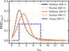 |
Fig. 1 Initial distribution of cluster formation redshifts. The different colors refer to different assumptions on the initial formation histories of GCs (solid lines) and NSCs (dashed lines). The initial redshift distribution of YCs is fixed in all models (gray solid line). The distributions are scaled such that the area subtended by the curve is 1. |
2.1.2 Black holes
In B-POP, the masses of BHs formed from single stars or in stellar binaries are drawn from catalogs generated using external stellar evolution tools. To ensure continuity with our previous works (Arca Sedda et al. 2023b), we adopted catalogs generated with MOBSE (Giacobbo & Mapelli 2018, 2020) covering metallicities in the range Z ∈ [0.0002, 0.02]. In particular, BH masses were extracted from either (i) a simple single stellar BH mass (SSBM) spectrum, corresponding to BHs formed from single stars, or (ii) a mixed single BH mass (MSBM) spectrum, which represents the population of BHs formed from binary stellar systems (Arca Sedda et al. 2023b). In all our runs BHs had a 50% probability to have a mass sampled from the MSBM or SSBM spectrum. We note that this subtly implied the inclusion in our dynamical models of effects related to primordial binary evolution, for example star mergers or accretion episodes (Arca Sedda et al. 2023b), a feature that may have a significant impact on the emergence of single and double IMBHs with a mass <300 M⊙ (see, e.g., Paiella et al. 2025). In both mass spectra the initial mass of a stellar-mass BH never exceeds the minimum IMBH mass, i.e., 100 M⊙. Nonetheless, additional features implemented in B-POP allow the user to assign BH masses in and beyond the pair instability supernova (PISN) range (Woosley 2017), for example assuming that their progenitors formed from one or multiple stellar collisions. We exploited this feature to explore the impact of different prescriptions for the early seeding of IMBHs, as detailed in Sects. 2.2.2, 2.2.3, and 2.3.
In our runs a BH (IMBH) can grow dynamically via repeated BBH mergers. After each merger the retention of the remnant is ensured only if its relativistic kick is lower than the escape velocity of the environment (see more on this in Sect. 2.2.4). This kick, which arises from asymmetries in GW emission prior to the merger, is primarily influenced by the mass ratio (q = m1/m2 < 1) of the BBH and the magnitude and relative alignment of the initial spins (Campanelli et al. 2007; Lousto & Zlochower 2008; Lousto et al. 2012). In our simulations we always assumed a BH (IMBH) to pair up with BHs which had not undergone any previous merger. Allowing higher-generation BH secondaries can, in principle, enhance hierarchical IMBH growth. However, such mergers are rare in relatively low-mass systems and are typically limited to the third generation by cluster expansion (Torniamenti et al. 2024). In general, multiple IMBHs are unlikely to form and grow within the same environment, except for clusters with a large fraction of primordial binaries, with extreme densities, or undergoing a hierarchical formation (see, e.g., Gürkan et al. 2006; Giersz et al. 2015; Mapelli 2016; Kovetz et al. 2018; Rodriguez et al. 2019; Anagnostou et al. 2020; González et al. 2021; Arca Sedda et al. 2023a; Rantala & Naab 2025). A prescription for the pairing up of BHs from different generation is under construction for the future public release of the code (Ugolini et al., in prep.).
Concerning the clusters’ BHs initial spins, we always assumed them to be distributed isotropically and with magnitudes following a Maxwellian distribution with dispersion σχ = 0.2. This distribution is consistent with the inferred spin distribution of merging BBHs observed by the LVK collaboration up to the O3 run (Abbott et al. 2023).
2.2 IMBH formation channels
In the following we briefly describe the processes regulating IMBH seeding and growth considered in this work, namely the stellar collision scenario and the hierarchical BBH merger scenario. We note that the two processes are not mutually exclusive; for example, an IMBH formed from the collision of a few massive stars can indeed grow further by merging with stellar BHs. For the sake of conciseness, we provide a more in-depth discussion about these mechanisms in Appendix A.2.
2.2.1 Cluster relaxation and core-collapse
Any gravitationally bound system undergoes dynamical relaxation driven by the continuous dynamical interactions among its constituents. In a star cluster, this process occurs over a timescale (Spitzer 1969; Binney & Tremaine 2008)
 (1)
(1)
called half-mass relaxation time, which depends on the cluster mass (Mcl) and the radius within which half of the cluster mass is contained, i.e., the half-mass radius (Rh,cl). Relaxation causes light stars to diffuse outward, carrying kinetic energy away from the core. This energy loss makes the core contract, which in turn increases the diffusion, creating a loop that leads the core to collapse. This phenomenon is commonly referred to as gravothermal instability (Spitzer 1969).
The contraction is finally reversed by the formation of hard binaries, that transfer kinetic energy to other core members through dynamical interactions and leads the core to bounce back. The core collapse process is, therefore, fundamentally governed by dynamical interactions between light and massive stars. These interactions also promote the segregation of the most massive stars in the cluster center on a timescale (Spitzer & Hart 1971; Portegies Zwart et al. 2004)
 (2)
(2)
where m is the mass of the sinking star,  is the average mass of a star in the cluster and
  is the average total number of stars assuming an initial cluster mass Mcl. For our simulations we fix
  and assume that the core collapse happens on a timescale equal to the segregation time of the most massive stars in the cluster population, i.e., for tcc ∼ ts(150 M⊙). Moreover, we define a lower bound for the core collapse timescales of tcc ∼ 0.2 trel (see also Portegies Zwart & McMillan 2002).
2.2.2 Runaway stellar collisions and IMBH seeds
If the core-collapse happens on timescales shorter than ∼3–5 Myr, which is the typical lifetime of BH massive stellar progenitors, it can trigger a chain of runaway stellar collisions and the formation of a VMS (Portegies Zwart & McMillan 2002) that may collapse into an IMBH.
The maximum mass of the VMS can be conveniently rewritten as a function of the initial cluster mass,
 (3)
(3)
with mseed and fc being the initial mass of the stellar seed and the effective fraction of colliding binaries in the cluster.
In general, Eq. (3) neglects the impact of stellar evolution processes which can affect both the amount of mass effectively accreted onto the growing VMS and the effect of metallicity on mass loss. For instance, strong stellar winds, typical of stellar populations with a metallicity Z ≳ 0.001, can effectively quench the VMS growth (e.g., Spera & Mapelli 2017; Iorio et al. 2023). Nonetheless, mass loss is expected to be nearly negligible for metal-poor stellar populations (see for instance Fig. 2 of Mapelli 2018). The final mass of the IMBH seeded by the VMS is also highly uncertain, although recent stellar evolution tracks for stars with masses up to 500–2000 M⊙ suggest that a relatively small fraction (<0.2–0.3) of the VMS mass is lost during the collapse to an IMBH if the metallicity is Z < 0.001 (see Fig. 4 in Costa et al. 2025). We also note that the ultimate fate of a star resulting from multiple stellar collisions may differ from that of a similar star born in isolation due to the different chemical stratification of the collided star and the additional rotation it may acquire during the collisions (Glebbeek et al. 2009; Costa et al. 2022; Ballone et al. 2023; Vergara et al. 2026).
2.2.3 Mild seeding scenario: Stellar collisions in dense star clusters
While the runaway scenario requires extreme conditions, in clusters with longer core collapse timescales numerical simulations have shown that several stellar collisions, often triggered by strong dynamical encounters among the population of primordial binaries, can lead to the rapid build-up of IMBH seeds with masses in the range 102 up to a few 103 M⊙(e.g., Mapelli 2016; Kremer et al. 2020; Di Carlo et al. 2021; Arca Sedda et al. 2023b; Rantala et al. 2024; Rantala & Naab 2025). Hence, we consider an additional scenario in which we assume a 20 % probability that a cluster denser than ρcl,0 > 105 M⊙ pc−3 and with metallicity Z < 0.001 forms a VMS, as recently suggested by Arca Sedda et al. (2023a) and Rantala et al. (2024); Rantala & Naab (2025). Under this scenario, we assign the mass of the VMS randomly between mVMS,min and mVMS,max, defined as
 (4)
(4)
 (5)
(5)
The lower bound on the minimum VMS mass matches the values in Table 1 of Rantala et al. (2024) which are derived from the cluster mass – maximum stellar mass relation in Yan et al. (2023). The upper bound on the maximum VMS mass at 2 × 10⁴ M⊙ serves as a conservative upper bound, given the uncertainties in mass loss and partial disruption of the star during each collision.
Although, in principle, this seeding mechanism can act in concert with the runaway one (Sect. 2.2.2), their development intrinsically depends on the cluster environment. In clusters that are prone to runaway collisions, the timescale for VMS build-up and collapse (∼2–5 Myr) is short enough to prevent long-term stellar collisions and to suggest that the VMS final product can grow by accreting stellar material in a tidal disruption event or by merging with other BHs. Clusters that may sustain a mild seeding, instead, are unlikely to undergo a runaway phase because stellar BHs, formed before the core-collapse, will likely settle in the centre and heat-up the core, preventing star-star mergers. For these reasons, we considered the two processes separately, as described in Sect. 2.3.
2.2.4 IMBH assembly via hierarchical binary black hole mergers
Aside from stellar collisions, an IMBH can also grow in a cluster via hierarchical BBH mergers, as summarized below.
Massive objects in a stellar population drift to the center of the parent cluster over a segregation timescale (Eq. (2)), with subsequent three-body (Lee 1995) and binary – single interactions (Goodman & Hut 1993), promoting the formation of hard binaries (Heggie 1975). Though these interactions get progressively rarer, they also become more violent and can impart a recoil to the BBH that may exceed the cluster escape velocity, leading to the premature ejection of the binary. However, if the hardening rate due to GW emission becomes dominant over the interaction rate before ejection, the BBH will merge inside the cluster. In such a case, the remnant is either expelled owing to the post-merger relativistic kick, or remains in the cluster possibly participating in another merger event. In either case, the BBH will undergo the merger only if the sum of cluster formation time, the time needed for the binary to form and harden, and the final merging time does not exceed a Hubble time. A BH typically needs to undergo a handful of mergers to reach the IMBH regime, an outcome possible only, in general, if the cluster’s escape velocity is sufficiently high to prevent its ejection.
2.3 Models descriptions
We explored three models based on different prescriptions for the IMBH seeding or the formation history of star clusters. The models are summarized in the following and in Table 2:
-
Model A: all clusters with a core collapse time shorter than 5 Myr and metallicity Z < 0.001 are assumed to trigger the formation of a VMS via runaway stellar collisions, followed by the seeding of an IMBH, as described in Sect. 2.2.2. We also invoke for the seeding a minimum cluster mass of 2 × 10⁴ M⊙ in order to have, on average, at least one seed massive star in the cluster (see Appendix B). The VMS mass (mVMS) is computed according to Eq. (3) assuming an initial star mass mseed = 150 M⊙ and an effective fraction of colliding binaries fc = 0.2. The resulting IMBH is assumed to retain 80% of the VMS mass, consistently with the findings of Costa et al. (2025) for these metallicities. We then follow the dynamical processes that may determine the pairing and merger of the IMBH with other stellar-mass BHs. If core collapse happens after 5 Myr, the runaway process is suppressed, and the IMBH formation can occur only through hierarchical BBH mergers (Sect. 2.2.4).
In this model, we assume YCs to follow the SFR from MF17, while for both GCs and NSCs we adopt the redshift distribution of KR13. The latter assumption supports the scenario in which NSCs share their formation history with GCs, as might occur if NSCs form through the (possibly rapid) merger of GCs migrated towards the galactic center via dynamical friction, a scenario commonly referred to as the migration scenario (Tremaine et al. 1975; Capuzzo-Dolcetta 1993; Neumayer et al. 2020, and references therein).
Model A′: this model adopts the same assumptions of Model A, except for the formation histories of GCs and NSCs. As with YCs, we assume NSCs to follow the SFR from MF17. This choice reflects a scenario in which NSCs form directly through star formation and gas infall occurring near the galactic center, a process commonly referred to as the in situ formation scenario (Loose et al. 1982). In addition, we sample the GCs formation redshift according to a Gaussian distribution with mean redshift µz = 3.2 and σz = 0.2 (Mapelli et al. 2022). This choice reflects theoretical models aimed at tracking the formation of Galactic GCs (see, e.g., EB18).
Model B: this model is based on the same set of assumptions of Model A regarding the cluster formation history, but assumes a mild seeding scenario in which stellar collisions can lead to the formation of a VMS with a 20% probability in clusters that are both metal-poor, Z < 0.001, and very dense, ρcl,0 > 105 M⊙ pc−3 (see also Sect. 2.2.3). As for the runaway seeding, we fix a minimum cluster mass (5 × 10³ M⊙) to ensure the presence of massive stellar seeds for the collisions (see Appendix B). The mass of the VMS is sampled as in Eq. (5) while we assume the IMBH to be 80% the mass of its progenitor. As in Model A simulation, if the cluster does not meet the seeding conditions we simply follow the dynamical evolution of a stellar-mass BH which may grow into an IMBH via hierarchical BBH mergers.
Models considered in this work and their main features.
3 Results
Hereafter, we refer to IMBHs formed from a stellar BH that underwent a chain of BBH mergers as hierarchical IMBHs, while we refer to IMBHs formed through direct collapse of a stellar collision product as IMBH seeds or seeded IMBHs. We note that IMBH seeds can also grow by further merging with stellar BHs.
3.1 Theoretical expectations
In Fig. 2 (left panel) we present the input distribution of initial masses and half-mass radii of YCs, GCs, and NSCs used in our simulations.
The runaway stellar collisions seeding, which we assume in Model A and A′, comprises all the environments falling on the left side of the dashed-dotted contour at tcc = 5 Myr. As shown in the plot, this seeding mechanism typically favors YCs as well as very light GCs and NSCs. Approximately 11% of YCs, 39% of GCs, and 20% of NSCs in B-POP fall within this runaway seeding region.
Conversely, the mild collision scenario, which we assume in Model B, selects the environments which fall above the gray dotted density contour at (half-mass) density ρcl,0 = 105 M⊙ pc−3. This seeding condition generally favors NSCs, which present the densest environments among the different cluster families. In this scenario we find that ∼19%, 9%, and 32% of YCs, GCs, and NSCs mass-radius distributions fall in the portion of the parameter space where ρcl,0 > 105 M⊙ pc−3. Assuming an additional 20 % seeding probability for these clusters (see more in Sect. 2.2.3) leads to ∼4%, 2%, and 6% of YCs, GCs, and NSCs being potential IMBH seeds hosts in Model B.
It should be noted, however, that the actual fraction of clusters producing IMBH seeds in both models depends critically on the metallicity, as we assume that the VMS progenitors are assembled only in clusters with Z < 0.001. The impact of metallicity is strictly linked to the clusters formation history and can significantly decrease the effective fraction of seeds hosts as we discuss in more details in Sect. 3.2.
The efficiency of hierarchical BBH mergers in assembling an IMBH is more complicated to define since many processes can actually lead to the ejection of the original BH during its growth. As a reference, in Fig. 2 we present, in different colors, the regions of the parameter space where a BBH (i) is ejected prior to merger due to a strong Newtonian recoil, (ii) merges and produces a BH which is then ejected by its relativistic kick, or (iii) the BBH is retained in the cluster but fails to merge within a Hubble time (see Appendix A.2 for further details). The first two regions are drawn comparing the magnitude of the recoils and kicks to the initial escape velocity of the host clusters. To evaluate the GW kicks we average over all possible spin configurations assuming them to be isotropically distributed in space, and sampling the spins magnitudes from our fiducial Maxwellian distribution (see more in Sect. 2). The last region is evaluated computing the average delay time between the BBH formation and merger in the cluster, and comparing it to a Hubble time. We adopt a 30 M⊙ − 30 M⊙ BBH as our reference system in all clusters, except when the cluster lies in the regime of runaway stellar collisions (i.e., tcc < 5 Myr). In that situation, we instead consider an IMBH-BH binary, with the primary mass set to m1 = 0.8 mVMS (Eq. (3)) and the secondary mass to m2 = 30 M⊙. For the stellar-mass BBH case, only the most massive NSCs lie outside the regions where the binary is either ejected or prevented from merging. In contrast, when an IMBH-BH binary forms from a seeded IMBH, the larger inertia of the system significantly reduces the probability of ejection, making retention within the cluster more likely even for YCs and GCs. This picture becomes, however, far more complicated when accounting for the temporal evolution of the host cluster which can strongly impact the IMBH formation and growth through the hierarchical channel. For instance, the cluster mass loss and expansion will drive clusters to wander downward and leftward in the Mcl,0–Rh,0 plane shown in Fig. 2, reducing the BH interaction rate and increasing the probability of BH ejection. This is especially the case of clusters with relaxation times comparable to the dynamical timescales over which the BBHs evolve. We explore all these aspects in more detail in the next section. Finally, in Fig. 2 we also provide a simple sketch of the processes contributing to the seeding and growth of an IMBH in a star cluster as well as the ejection mechanisms mentioned above.
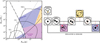 |
Fig. 2 Left panel: initial cluster mass and half-mass radius for YCs (bottom left area), GCs (central area), and NSCs (upper right area). The cluster distributions are cut at the 99% contour. Clusters with tcc < 5 Myr lie below the dot-dashed black line; those with central density ρcl,0 > 105 M⊙ pc−3 are above the shaded dotted gray line. We also identify regions of the parameter space in which (i) a BBH binary is ejected before merging due to strong Newtonian recoils (in pink), (ii) the merger remnant is typically kicked out of the cluster due to its relativistic kick (in purple), (iii) the BBH merger time exceeds a Hubble time (in yellow). Right panel: schematic overview of a BH dynamical growth in a star cluster. The colored boxes refer to the regions highlighted in the left plot. |
3.2 Demographics
We find that only a small fraction of the 108 BH realizations produces an IMBH: about ∼0.6% in Model A, ∼0.4% in Model A′, and ∼0.1% in Model B. In all cases, the overwhelming majority of IMBHs originates from stellar collision seeds. Specifically, these IMBHs represent ∼97–98% of the whole IMBH population in Models A and A′, and ∼88% in Model B. Hence, in all our simulations stellar collisions appear to be the primary drivers of IMBH formation in star clusters. The overall IMBH fractions remain modest mainly due to the imposed constraint on the metallicity threshold that we require for the formation of a VMS via stellar collisions. It is also important to note that, in our simulations, YCs, GCs, and NSCs are assumed to be equally abundant. Therefore, these fractions do not reflect the true relative proportions of different cluster families in the Universe, which remain highly uncertain. For reference, the Milky Way hosts one NSC, ∼200 GCs (Harris 1996; Minniti et al. 2017), and possibly up to ∼103 massive YCs clusters (Larsen 2009).
To quantify the IMBH formation efficiency within each cluster family, we report in Table 3 the final IMBH populations, distinguishing between their formation channel (hierarchical or seeded) and the host cluster type (YCs, GCs, NSCs). The percentages shown for each mechanism are computed relative to the total number of clusters belonging to the corresponding family. From Table 3 it is clear that seeding via stellar collisions is consistently more efficient than hierarchical growth, by at least one order of magnitude, regardless of the cluster type. The environments in which this mechanism is more frequent, however, depend strongly on both the seeding conditions (Model A vs. Model B) and the assumed cluster formation histories (Model A vs. Model A′). For instance, in Model A, GCs are more likely to be hosting a seed thanks to their shorter core collapse times, whereas in Model B the seeding is restricted to very dense clusters, hence IMBH seeds are formed more frequently in NSCs. A direct comparison between Models A and A′ further illustrates the impact of formation history. In Model A′, only about 0.05% of GCs produce an IMBH seed, compared to ∼0.8% of NSCs. This trend is reversed in Model A, where GCs are nearly twice as likely as NSCs to host a seed. The difference arises because, in Model A′, GCs statistically form at lower redshifts than in Model A, and thus tend to have higher metallicities, often exceeding the threshold for runaway or mild stellar collisions. While NSCs also tend to form later in Model A′, their redshift distribution extends up to z ≳ 10, broader than that of GCs. This wider redshift range partly offsets the metallicity constraint, allowing a nonnegligible fraction of NSCs to still meet the seeding conditions.
Across all three models, hierarchical IMBH formation is efficient only in NSCs, while YCs and GCs produce virtually no IMBHs through this channel (see Table 3). This is because only NSCs reach escape velocities high enough to retain stellar-mass BHs against the typical dynamical recoils and relativistic kicks they experience during their growth (see Sect. 3.3.1).
The differences observed for the IMBH formation efficiency across formation mechanisms and cluster environments also impact the final population of mergers involving IMBHs observed in our simulations. We discuss the properties these mergers in Appendix C.
Global percentages of IMBHs in our simulations.
3.3 IMBHs at low redshifts: Models and observations
3.3.1 Retention efficiency and ejection mechanisms
At redshift z = 0, only around 33% (Model A), 39% (Model A′), and 61% (Model B) of all IMBHs forming in the simulations are retained in their clusters. In general, the IMBHs in our simulations can be ejected by means of three different processes: (i) Newtonian recoils, which expel an IMBH-BH binary as a result of strong binary-single interaction with the other BHs in the cluster, (ii) relativistic kicks, which eject an IMBH remnant after the binary merged, and (iii) the complete evaporation of the IMBH host cluster. The latter process mainly affects light clusters with short relaxation times which completely disrupt within a Hubble time, releasing their IMBHs in the field (see also Sect. 3.3.2).
In Table 4, we summarize the final fate of IMBHs in our simulations, categorized by formation mechanism, cluster family, and ejection process. We also report the fraction of IMBHs retained at z = 0, with all percentages normalized to the total number of IMBHs formed in each cluster type and formation scenario. We focus on the comparison between Model A and B, as Model A′ exhibits trends similar to Model A. While Models A and A′ differ in the total number of IMBH seeds due to the different choice of initial metallicity (redshift) distributions (Sect. 3.2), the relative fractions of IMBHs that are ejected or retained remain essentially unchanged. This is because these fractions are primarily set by the initial BH and IMBH seed properties and by the escape velocities and dynamical evolution of their host clusters, which are identical in both models. In addition, for hierarchical IMBHs we only refer to NSCs, since the fractions of IMBHs formed in YCs and GCs through this channel are always smaller than 0.01% (see Table 3).
Model B exhibits a substantially higher fraction of IMBH seeds retained at z = 0 compared to Model A. This arises from the higher-density threshold imposed for IMBH seeding in Model B, which preferentially selects host clusters with larger escape velocities than those in Model A. In both models, IMBHs are primarily ejected through post-merger relativistic kicks. This is particularly evident for hierarchical IMBHs, which are retained at z = 0 in less than 15% of the times. In addition to dynamical ejection mechanisms, such as kicks or recoils, we find that the premature evaporation of YCs quenches the growth of IMBH seeds in 11–17% of cases, depending on the model. In Sect. 4.1 we discuss possible observational implications for this population of orphan IMBHs.
Final fate of IMBHs at redshift z = 0.
3.3.2 Comparison to low-redshift IMBH candidates
In Fig. 3, we compare the IMBH population retained at z = 0 in our simulations with several observations of IMBH candidates in local GCs (Lützgendorf et al. 2013b; Kızıltan et al. 2017; Häberle et al. 2024), in extragalactic clusters from potential tidal distruption events (Lin et al. 2018), in galactic nuclei (Graham & Spitler 2009; Neumayer & Walcher 2012; Kormendy & Ho 2013), in dwarf galaxies, ultra-compact dwarf galaxies (UCDs) and low-mass active galactic nuclei (AGNs; Reines & Volonteri 2015; Chilingarian et al. 2018; Nguyen et al. 2018). In the following we restrict the analysis to Model A and Model B, as Model A and Model A′ produce results broadly consistent with each other. Model A is shown in the left panel of Fig. 3, while Model B is displayed in the right panel.
In Model A, IMBH seeds can form only in clusters with a core collapse time tcc ≲ 5 Myr, a condition that translates into an upper limit on the clusters relaxation times and, consequently, their lifetime. This effect is evident in Fig. 3 for YCs and low-mass GCs, which in our simulations either evaporate before z = 0 (see also Table 4) or undergo substantial mass loss, retaining IMBHs with typical final mass ratios MIMBH/Mcl ≳ 0.1. Conversely, hierarchical IMBHs are retained only in clusters with final masses ≳107 M⊙ and exhibit typical mass ratios MIMBH/Mcl ≲ 10−2, filling a region of the cluster mass–IMBH mass plane partly populated by observed NSCs. The growth proceeds uninterrupted in the densest clusters with final masses > 108 M⊙, generally leading to the exhaustion of the BH reservoir. These clusters show notable similarities with more complex stellar systems, such as UCDs and light low-mass AGNs. In Model A we observe a distinct gap around Mcl ∼ 107, M⊙ between the seeded and hierarchical populations, which lie to the left and right of the gap, respectively. The gap emerges from the combined effect of the seeding conditions and the inefficiency of hierarchical BBH mergers in clusters falling in that mass range. For completeness, in Appendix D we also discuss how the gap may be affected assuming GCs to be more massive and compact at birth. The IMBH mass – host mass relation changes significantly in Model B. In this model the seeded and hierarchical retained populations fill homogeneously the cluster mass range ∼103–109 M⊙ and clearly overlap with the masses of putative IMBHs observed in galactic and extragalactic GCs, as well as NSCs in the local Universe. In both models we observe a tail of light IMBHs (∼100 M⊙) in clusters heavier than ∼105 M⊙. These IMBHs are retained as part of IMRIs with merging times exceeding a Hubble time.
The clear difference between the two seeding models at z = 0 raises several interesting points. First, it highlights the limited role of runaway stellar collisions in favoring the growth of IMBHs heavier than 104–105 M⊙. Second, it clearly shows the low efficiency of the hierarchical BBH merger scenario in explaining low-redshift IMBHs observations, except in very massive and dense hosts (≳107 M⊙ pc−3). Third, it suggests that a hybrid scenario in which an IMBH seed forms from a few collisions among massive stars (e.g., triggered by binary-single and binary-binary interactions) and possibly further grows by merging with lighter BHs, as in Model B, may be a promising dynamical formation channel for IMBHs in GC-like environments.
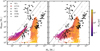 |
Fig. 3 Clusters hosting an IMBH at z = 0 in Model A (left panel) and Model B (right panel) compared to different classes of IMBH host candidate observations. We note that the masses reported for low-mass AGNs refer to the host galaxy mass (up to ∼ 100 times higher than the mass of the galactic nuclei). The gray dashed line shows the theoretical prediction for the initial mass of an IMBH seeded via stellar collisions (Eq. (3) in the left panel and Eq. (5) in the right panel). |
4 Discussion
In the following we present some practical applications of our models to the study of IMBHs in YCs and GCs. In particular, we analyze the implications of premature IMBH ejection from YCs on wandering IMBHs in the Milky Way and other galaxy halos, and investigate the origin of Galactic GCs through potential IMBH signatures. These discussions will form the basis for more detailed studies in forthcoming papers.
4.1 Young clusters and wandering IMBHs
As discussed in Sect. 3.3.2, metal-poor YCs with short relaxation time can form IMBHs via stellar collisions. However, many of these IMBHs are likely to be ejected shortly after formation due to Newtonian recoils, post-merger relativistic kicks, or the evaporation of their host clusters. In this section we briefly explore whether a population of IMBHs formed in Milky Way young and open clusters could remain trapped in the Galactic potential and now wander across the Milky Way.
To explore this scenario and filter out statistical fluctuations, we resimulated 5 × 10⁷ BBHs in YCs, focusing on the runaway collision scenario (Model A) and the mild collision scenario (Model B). In all models, IMBHs are either ejected during their build-up or are retained until the cluster evaporates via internal relaxation and tidal disruption operated by the galactic potential. Upon cluster dispersal, the IMBH is gently released in the galactic environment, where it will keep following the original orbit of its former host up to a Hubble time. Clusters formed sufficiently close to the center of the galaxy can also drift inward and bring their IMBHs to the galactic nucleus, a process that possibly impacts both the growth of NSCs and SMBHs (Tremaine et al. 1975; Capuzzo-Dolcetta 1993; Ebisuzaki et al. 2001; Portegies Zwart et al. 2006; Antonini et al. 2012; Arca Sedda et al. 2015; Arca Sedda & Gualandris 2018).
Depending on the ejection mechanism, the IMBH is released in the field with a different velocity. IMBHs ejected via GW relativistic kicks receive a median kick of 20 km/s, with tails up to 103 km/s, those ejected through dynamical interactions attain velocities of at most a few km/s, while for those released by evaporating clusters we assume a velocity ∼0 km/s. The ejection mechanism also determines whether the IMBH is expelled as a single object (e.g., in the aftermath of a BBH merger) or as a binary (in case of dynamical ejections and evaporated clusters). Regardless of the ejection mechanism, IMBH ejection velocities are generally much lower than the typical escape velocity estimated for the present-time Milky Way disk (∼500 km/s; see for reference Hunt & Vasiliev 2025), thus suggesting that expelled IMBHs should remain anchored to the Milky Way gravitational field.
To constrain the number of IMBHs produced in YCs and now wandering the Milky Way, we assume that the Galactic potential at the time of ejection resembles its present-day configuration. As a reference, we adopt the MWPotential2014 model implemented in galpy (Bovy 2015), which combines the contributions of a bulge, a disk, and a dark matter halo.
Observations of Milky Way disk clusters suggest that ∼19 000 YCs with masses ≳104 M⊙ may have formed over ∼10 Gyr (Larsen 2009). Using our catalogs, we generate 5000 realizations of this population, drawing 19 000 YCs per realization with initial masses above 104 M⊙. Each YC (IMBH) is assigned a random position in the galactic plane, and the number of IMBHs retained is determined by comparing their final recoil or kick to the Galactic escape velocity. Our analysis suggests that 273 ± 8 (26 ± 2) wandering IMBHs form in Model A (Model B), among which roughly ∼20–25% are in IMBH-BH systems (48 ± 4 for Model A and 8 ± 1 for Model B). In both models, the majority of these IMBHs have masses around ∼350 M⊙ and ejection velocities vej < 102 km/s.
The potential existence of these IMBHs in the Galaxy could have interesting observational implications. For instance, single or binary IMBHs might be detectable through microlensing (Paczynski 1986). IMBHs ejected from the cluster could capture luminous companions, allowing astrometric measurements to reveal their presence in the binary, as demonstrated by Gaia’s discovery of BH–star systems (El-Badry et al. 2023a,b; Chakrabarti et al. 2023; Tanikawa et al. 2024; Gaia Collaboration 2024). Furthermore, ejected IMBH–BH binaries may emit low-frequency gravitational waves detectable by interferometers such as LISA (see, e.g., Arca Sedda et al. 2021).
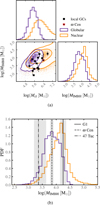 |
Fig. 4 Comparison of simulated IMBH candidates in Model B with observational data. (a) Corner plot showing the GCs (purple) and NSCs (orange) clusters in our simulations hosting an IMBH at z = 0, compared to observations of potential IMBHs in Milky Way globular clusters and G1. (b) One-dimensional IMBH mass distribution, compared to estimated masses for G1 and 47 Tuc. |
4.2 Galactic globular clusters hosting IMBHs and their (mis)classification
As discussed in Sect. 3.3.2, stellar collisions can explain potential IMBH observations at z = 0 in clusters with masses below ∼107 M⊙. However, the agreement between our simulations and candidate GCs hosts (Lützgendorf et al. 2013b; Kızıltan et al. 2017; Häberle et al. 2024) depends strongly on the assumed IMBH seeding model. Figure 3 shows that a runaway stellar collision scenario (Model A) struggles to reproduce these observations, whereas a milder stellar collision scenario (Model B) aligns significantly better with the data.
Focusing on Model B, we find that both GCs and NSCs can partially recover the same host–IMBH masses inferred for these observations (Fig. 4). To quantify this, we introduce a simple Bayesian framework to evaluate whether local IMBH host candidates are more likely GCs or NSCs, offering a systematic approach for studying the Milky Way’s GCs. This is particularly relevant since the Galactic population of GCs is expected to be mixed. Theoretical models and observations indeed suggest that a fraction of the Milky Way’s GCs formed in situ, while ∼30– 35% were accreted during galaxy mergers (see, e.g., Massari et al. 2019), with some of the latter possibly being stripped galactic nuclei. Since our simulations reveal clear links between the properties of a cluster and its IMBH, they provide a powerful tool to differentiate between genuine GCs and former NSCs among local IMBH hosts.
To summarize, our goal is to use the Bayes factor to compare two competing hypotheses for the nature of the observed IMBH hosts:
HGC: the observed IMBH host is a GC;
HNSC: the observed IMBH host is a NSC.
As already mentioned, we restrict our analysis to Model B simulation (right panel of Fig. 3), which shows the most significant overlap with the observed candidates. From this simulation we obtain discrete samples of the logarithm of the intrinsic cluster mass and IMBH mass, i.e., {log(Mcl), log(MIMBH)}. To convert these samples into continuous probability densities we smooth them using a gaussian kernel density estimator (KDE). Figure 4 shows a zoom-in of these simulated distributions together with the inferred cluster and IMBH masses of a set of known Milky Way and local GCs host candidates (black squares). These masses are also listed in Table 5. We gather these estimates from a collection of different studies (Lützgendorf et al. 2013b; Kızıltan et al. 2017; Häberle et al. 2024; Bañares-Hernández et al. 2025) as follows. For the clusters with only upper limits on IMBH masses in Lützgendorf et al. (2013b), we conservatively treat these limits as representative values. For ω Centauri (ω Cen), we rely instead on two recent and somewhat conflicting analyses. Häberle et al. (2024) infer a lower limit of ∼8200 M⊙ based on stellar kinematics, whereas Bañares-Hernández et al. (2025) favor an extended central mass of ∼2–3 × 10⁵ M⊙, setting a lower limit of ∼6000 M⊙ for an IMBH. To bracket these uncertainties, we model the IMBH mass in ω Cen as uniformly distributed between 6000 and 8200 M⊙. Finally, for 47 Tucanae (47 Tuc) we adopt the cluster and IMBH mass estimates reported by Kızıltan et al. (2017). We emphasize, however, that the existence of an IMBH in 47 Tuc is still controversial, as multiple studies have demonstrated that a highly concentrated population of stellar-mass BHs in the cluster core can account for its observed dynamical properties without invoking an IMBH (see, e.g., Mann et al. 2019; Hénault-Brunet et al. 2020). For each set of inferred masses, we assign a posterior probability distribution function, which we approximate as a two-dimensional Gaussian with means and standard deviations given by the reference values in Table 5.
In Appendix E, we derive an approximated expression of the Bayes factor relative to a single observation assuming that the likelihood is effectively the same for HGC and HNSC, and exploiting the fact that the likelihood can be derived directly from the posterior of {log(Mcl), log(MIMBH)} if the prior is sufficiently broad and uniform. The values of the Bayes factors’ logarithms for each host candidate are listed in the last column of Table 5 as log  . We note that the rows of Table 5 are ordered according to log
  in descending order, with positive (negative) values supporting a NSC (GC) hypothesis. In particular, we can consider log
  as strongly pointing towards a NSC (GC) nature of the cluster (Jeffreys 1939). Two notable cases which emerge from our simple analysis are the G1 cluster, which orbits the Andromeda galaxy, and ω Cen in the Milky Way, both showing substantial preference for a NSC origin. G1 is hypothesized to be the disrupted nucleus of a dwarf galaxy that merged with Andromeda, a scenario supported by its broad stellar metallicity distribution (see, e.g., Ma et al. 2007). Similarly, ω Cen, the most massive cluster in the Milky Way, is also one possible example of an accreted nuclei (Hilker & Richtler 2000; Ibata et al. 2019), though the presence of an IMBH in this cluster has long been debated. Most clusters, like 47 Tuc, show a slight or negligible preference to the NSC or GC hypothesis. For reference, in Fig. 4 we also present a zoom-in of the IMBH mass distributions in GCs and NSCs and the putative masses of the IMBHs contained in G1, ω Cen and 47 Tuc. We note that, while G1 falls on the peak of the NSCs distribution found in our simulations, the ω Cen IMBH mass is more compatible with the IMBHs found in GCs. Nevertheless the large mass of this cluster ultimately determines its preference towards a NSC origin.
Bayes factor comparing a nuclear origin versus a globular origin for local IMBH host candidates.
5 Conclusions
We investigated the formation and growth mechanisms of IMBHs in young (YCs), globular (GCs), and nuclear (NSCs) clusters by means of the new semianalytic code B-POP (Arca Sedda & Benacquista 2019; Arca Sedda et al. 2023b; Arca Sedda et al., in prep.). We focused on the potential formation of IMBHs through two mutually nonexclusive channels, namely (i) the collapse of very massive stars (VMSs) resulting from repeated stellar collisions and (ii) hierarchical BBH mergers. For the first channel, we adopted two models: Model A, assuming VMS formation via runaway stellar collisions in clusters with short core-collapse times (tcc < 5 Myr; Portegies Zwart & McMillan 2002), and Model B, invoking a mild collision scenario in which multiple stellar collisions in extremely dense clusters drive the VMSs formation (ρcl,0 > 105 M⊙ pc−3) and motivated by recent N-body simulations (Arca Sedda et al. 2023a; Rantala & Naab 2025). In both cases we restricted the seeding to metal-poor environments (Z < 0.001) to avoid strong stellar-wind mass loss. Furthermore, we tested a separate scenario using the same seeding as Model A, but with alternative redshift distributions for NSCs and GCs (Model A′), to examine the effects of clusters formation histories on IMBH assembly.
Our main results can be summarized as follows:
We show that seeding conditions and cluster formation histories strongly shape the IMBH formation efficiency across cluster families. The runaway stellar collision scenario (Model A), which favors systems with short core-collapse times, maximizes the efficiency in GCs. Conversely, the mild collision scenario (Model B) is the most efficient in NSCs, which comprise the densest clusters. In Model A′ NSCs prove to be much more efficient at producing IMBH seeds compared to GCs, owing to their broader distributions in redshift and metallicity, which extends down to Z < 0.001. Hierarchical IMBHs form efficiently only in NSCs;
We observe a marked gap in the cluster mass–IMBH mass plane at Mcl ∼ 107, M⊙ for the population of IMBHs retained at z = 0 in Model A. This scarcity of IMBH hosts results from the combined effects of the seeding conditions and the inefficiency of the hierarchical channel IMBH formation channel. In contrast, Model B presents a homogeneous population of retained IMBHs which smoothly transitions from IMBHs seeded by stellar collisions to those assembled hierarchically via BBH mergers. These IMBHs have a clear overlap with potential observations of IMBHs in galactic GCs.
Additionally, we discussed possible implications for IMBHs in YCs and GCs:
We showed that if stellar collisions are an efficient mechanism for IMBH formation, we likely expect a subpopulation of ejected IMBH seeds wandering in the potential well of Milky Way-like galaxies. The presence of such IMBHs (as single objects or in binaries) could be probed through different observational channels, such as astrometric measurements of a potential stellar companion (similarly to Gaia-BH1, Gaia-BH2, and Gaia-BH3 El-Badry et al. 2023a,b; Chakrabarti et al. 2023; Tanikawa et al. 2024; Gaia Collaboration 2024), microlensing (Paczynski 1986), or GW emission signatures (Arca Sedda et al. 2021);
We discuss a simple Bayesian framework that exploits the correlations found in our simulations between the clusters and IMBHs masses to probe the nature of Milky Way IMBH host candidates. This is particularly interesting as some of the Milky Way GCs (e.g., ω Cen) are believed to actually be stripped nuclei of galaxies that interacted with our galaxy in the past. We apply this approach comparing the systems found in Model B to the inferred masses in Lützgendorf et al. (2013b); Kızıltan et al. (2017); Häberle et al. (2024); Bañares-Hernández et al. (2025). We find that most clusters lie in a region where the GCs and NSCs hypotheses are equally probable with the exception of the G1 cluster in the Andromeda galaxy and ω Cen, which strongly support a NSC origin.
Overall, our work highlights the critical role of stellar collisions in producing IMBHs over a broad range of clusters. Moreover, we propose possible ways of probing the presence of such IMBHs and of disentangling their formation mechanisms and the formation histories of their hosts. We also emphasize the fundamental importance of simultaneously considering the codependences among different formation mechanisms, cluster families, and their evolutionary histories, as well as environmental factors, to effectively investigate IMBH production and growth. In this context, the B-POP code represents a valuable tool for these kinds of studies as it integrates all these aspects within a flexible and efficient framework.
Acknowledgements
The authors acknowledge Gor Oganesyan, Filippo Santoliquido, and Konstantinos Kritos for useful discussion and comments. MAS acknowledges funding from the European Union’s Horizon 2020 research and innovation programme under the Marie Skłodowska-Curie grant agreement No. 101025436 (project GRACE-BH). MAS and CU acknowledge financial support from the MERAC Foundation under the 2023 MERAC prize and support to research. This research made use of NUMPY (Harris et al. 2020), SCIPY (Virtanen et al. 2020), PANDAS (Pandas Development Team 2020). For the plots we used MATPLOTLIB (Hunter 2007).
References
- Abac, A., Abramo, R., Albanesi, S., et al. 2025a, arXiv e-prints [arXiv:2503.12263] [Google Scholar]
- Abac, A. G., Abouelfettouh, I., Acernese, F., et al. 2025b, ApJ, 993, L25 [Google Scholar]
- Abbott, R., Abbott, T. D., Abraham, S., et al. 2020, Phys. Rev. Lett., 125, 101102 [Google Scholar]
- Abbott, R., Abbott, T. D., Acernese, F., et al. 2023, Phys. Rev. X, 13, 011048 [NASA ADS] [Google Scholar]
- Ajith, P., Seoane, P. A., Arca Sedda, M., et al. 2025, J. Cosmology Astropart. Phys., 2025, 108 [Google Scholar]
- Anagnostou, O., Trenti, M., & Melatos, A. 2020, PASA, 37, e044 [Google Scholar]
- Antonini, F., & Rasio, F. A. 2016, ApJ, 831, 187 [Google Scholar]
- Antonini, F., & Gieles, M. 2020, MNRAS, 492, 2936 [CrossRef] [Google Scholar]
- Antonini, F., Capuzzo-Dolcetta, R., Mastrobuono-Battisti, A., & Merritt, D. 2012, ApJ, 750, 111 [NASA ADS] [CrossRef] [Google Scholar]
- Arca Sedda, M., & Gualandris, A. 2018, MNRAS, 477, 4423 [NASA ADS] [CrossRef] [Google Scholar]
- Arca Sedda, M., & Benacquista, M. 2019, MNRAS, 482, 2991 [NASA ADS] [Google Scholar]
- Arca Sedda, M., Capuzzo-Dolcetta, R., Antonini, F., & Seth, A. 2015, ApJ, 806, 220 [NASA ADS] [CrossRef] [Google Scholar]
- Arca Sedda, M., Berry, C. P. L., Jani, K., et al. 2020a, Class. Quant. Grav., 37, 215011 [Google Scholar]
- Arca Sedda, M., Mapelli, M., Spera, M., Benacquista, M., & Giacobbo, N. 2020b, ApJ, 894, 133 [NASA ADS] [CrossRef] [Google Scholar]
- Arca Sedda, M., Amaro Seoane, P., & Chen, X. 2021, A&A, 652, A54 [NASA ADS] [CrossRef] [EDP Sciences] [Google Scholar]
- Arca Sedda, M., Kamlah, A. W. H., Spurzem, R., et al. 2023a, MNRAS, 526, 429 [NASA ADS] [CrossRef] [Google Scholar]
- Arca Sedda, M., Mapelli, M., Benacquista, M., & Spera, M. 2023b, MNRAS, 520, 5259 [NASA ADS] [CrossRef] [Google Scholar]
- Bañares-Hernández, A., Calore, F., Martin Camalich, J., & Read, J. I. 2025, A&A, 693, A104 [NASA ADS] [CrossRef] [EDP Sciences] [Google Scholar]
- Ballone, A., Costa, G., Mapelli, M., et al. 2023, MNRAS, 519, 5191 [NASA ADS] [CrossRef] [Google Scholar]
- Barber, J., & Antonini, F. 2024, arXiv e-prints [arXiv:2410.03832] [Google Scholar]
- Baumgardt, H., & Hilker, M. 2018, MNRAS, 478, 1520 [Google Scholar]
- Bavera, S. S., Fragos, T., Qin, Y., et al. 2020, A&A, 635, A97 [NASA ADS] [CrossRef] [EDP Sciences] [Google Scholar]
- Binney, J., & Tremaine, S. 2008, Galactic Dynamics: Second Edition, 2 rev. edn. (Princeton University Press) [Google Scholar]
- Bovy, J. 2015, ApJS, 216, 29 [NASA ADS] [CrossRef] [Google Scholar]
- Campanelli, M., Lousto, C. O., Zlochower, Y., & Merritt, D. 2007, Phys. Rev. Lett., 98, 231102 [Google Scholar]
- Capuzzo-Dolcetta, R. 1993, ApJ, 415, 616 [NASA ADS] [CrossRef] [Google Scholar]
- Chakrabarti, S., Simon, J. D., Craig, P. A., et al. 2023, AJ, 166, 6 [NASA ADS] [CrossRef] [Google Scholar]
- Chilingarian, I. V., Katkov, I. Y., Zolotukhin, I. Y., et al. 2018, ApJ, 863, 1 [Google Scholar]
- Colpi, M., Mapelli, M., & Possenti, A. 2003, ApJ, 599, 1260 [Google Scholar]
- Costa, G., Ballone, A., Mapelli, M., & Bressan, A. 2022, MNRAS, 516, 1072 [NASA ADS] [CrossRef] [Google Scholar]
- Colpi, M., Danzmann, K., Hewitson, M., et al. 2024, arXiv e-prints [arXiv:2402.07571] [Google Scholar]
- Costa, G., Shepherd, K. G., Bressan, A., et al. 2025, A&A, 694, A193 [NASA ADS] [CrossRef] [EDP Sciences] [Google Scholar]
- D’Amico, N., Possenti, A., Fici, L., et al. 2002, ApJ, 570, L89 [CrossRef] [Google Scholar]
- Di Carlo, U. N., Mapelli, M., Pasquato, M., et al. 2021, MNRAS, 507, 5132 [NASA ADS] [CrossRef] [Google Scholar]
- Ebisuzaki, T., Makino, J., Tsuru, T. G., et al. 2001, ApJ, 562, L19 [NASA ADS] [CrossRef] [Google Scholar]
- El-Badry, K., Quataert, E., Weisz, D. R., Choksi, N., & Boylan-Kolchin, M. 2019, MNRAS, 482, 4528 [Google Scholar]
- El-Badry, K., Rix, H.-W., Cendes, Y., et al. 2023a, MNRAS, 521, 4323 [NASA ADS] [CrossRef] [Google Scholar]
- El-Badry, K., Rix, H.-W., Quataert, E., et al. 2023b, MNRAS, 518, 1057 [Google Scholar]
- Ferraro, F. R., Possenti, A., Sabbi, E., et al. 2003, ApJ, 595, 179 [NASA ADS] [CrossRef] [Google Scholar]
- Fryer, C. L., Belczynski, K., Wiktorowicz, G., et al. 2012, ApJ, 749, 91 [Google Scholar]
- Gaia Collaboration (Panuzzo, P., et al.) 2024, A&A, 686, L2 [NASA ADS] [CrossRef] [EDP Sciences] [Google Scholar]
- Gatto, M., Ripepi, V., Bellazzini, M., et al. 2021, MNRAS, 507, 3312 [NASA ADS] [CrossRef] [Google Scholar]
- Gebhardt, K., Rich, R. M., & Ho, L. C. 2005, ApJ, 634, 1093 [NASA ADS] [CrossRef] [Google Scholar]
- Georgiev, I. Y., Böker, T., Leigh, N., Lützgendorf, N., & Neumayer, N. 2016, MNRAS, 457, 2122 [Google Scholar]
- Giacobbo, N., & Mapelli, M. 2018, MNRAS, 480, 2011 [Google Scholar]
- Giacobbo, N., & Mapelli, M. 2020, ApJ, 891, 141 [NASA ADS] [CrossRef] [Google Scholar]
- Gieles, M., Balbinot, E., Yaaqib, R. I. S. M., et al. 2018, MNRAS, 473, 4832 [CrossRef] [Google Scholar]
- Giersz, M., Leigh, N., Hypki, A., Lützgendorf, N., & Askar, A. 2015, MNRAS, 454, 3150 [Google Scholar]
- Glebbeek, E., Gaburov, E., de Mink, S. E., Pols, O. R., & Portegies Zwart, S. F. 2009, A&A, 497, 255 [NASA ADS] [CrossRef] [EDP Sciences] [Google Scholar]
- González, E., Kremer, K., Chatterjee, S., et al. 2021, ApJ, 908, L29 [CrossRef] [Google Scholar]
- González Prieto, E., Weatherford, N. C., Fragione, G., Kremer, K., & Rasio, F. A. 2024, ApJ, 969, 29 [CrossRef] [Google Scholar]
- Goodman, J., & Hut, P. 1993, ApJ, 403, 271 [Google Scholar]
- Graham, A. W., & Spitler, L. R. 2009, MNRAS, 397, 2148 [NASA ADS] [CrossRef] [Google Scholar]
- Gültekin, K., Miller, M. C., & Hamilton, D. P. 2004, ApJ, 616, 221 [Google Scholar]
- Gürkan, M. A., Fregeau, J. M., & Rasio, F. A. 2006, ApJ, 640, L39 [Google Scholar]
- Häberle, M., Neumayer, N., Seth, A., et al. 2024, Nature, 631, 285 [CrossRef] [Google Scholar]
- Harris, W. E. 1996, AJ, 112, 1487 [Google Scholar]
- Harris, C. R., Millman, K. J., van der Walt, S. J., et al. 2020, Nature, 585, 357 [NASA ADS] [CrossRef] [Google Scholar]
- Heggie, D. C. 1975, MNRAS, 173, 729 [NASA ADS] [CrossRef] [Google Scholar]
- Hénault-Brunet, V., Gieles, M., Strader, J., et al. 2020, MNRAS, 491, 113 [CrossRef] [Google Scholar]
- Hilker, M., & Richtler, T. 2000, A&A, 362, 895 [NASA ADS] [Google Scholar]
- Hunt, J. A. S., & Vasiliev, E. 2025, arXiv e-prints [arXiv:2501.04075] [Google Scholar]
- Hunter, J. D. 2007, Comput. Sci. Eng., 9, 90 [NASA ADS] [CrossRef] [Google Scholar]
- Ibata, R. A., Bellazzini, M., Malhan, K., Martin, N., & Bianchini, P. 2019, Nat. Astron., 3, 667 [Google Scholar]
- Iorio, G., Mapelli, M., Costa, G., et al. 2023, MNRAS, 524, 426 [NASA ADS] [CrossRef] [Google Scholar]
- Izquierdo-Villalba, D., Lupi, A., Regan, J., Bonetti, M., & Franchini, A. 2023, arXiv e-prints [arXiv:2311.03152] [Google Scholar]
- Jeffreys, H. 1939, Theory of Probability [Google Scholar]
- Kamann, S., Husser, T. O., Brinchmann, J., et al. 2016, A&A, 588, A149 [NASA ADS] [CrossRef] [EDP Sciences] [Google Scholar]
- Kamann, S., Wisotzki, L., Roth, M. M., et al. 2014, A&A, 566, A58 [NASA ADS] [CrossRef] [EDP Sciences] [Google Scholar]
- Katz, H., & Ricotti, M. 2013, MNRAS, 432, 3250 [Google Scholar]
- Kızıltan, B., Baumgardt, H., & Loeb, A. 2017, Nature, 542, 203 [Google Scholar]
- Kormendy, J., & Ho, L. C. 2013, ARA&A, 51, 511 [NASA ADS] [CrossRef] [Google Scholar]
- Kovetz, E. D., Cholis, I., Kamionkowski, M., & Silk, J. 2018, Phys. Rev. D, 97, 123003 [Google Scholar]
- Kremer, K., Spera, M., Becker, D., et al. 2020, ApJ, 903, 45 [NASA ADS] [CrossRef] [Google Scholar]
- Kritos, K., Strokov, V., Baibhav, V., & Berti, E. 2024, Phys. Rev. D, 110, 043023 [Google Scholar]
- Kroupa, P. 2001, MNRAS, 322, 231 [NASA ADS] [CrossRef] [Google Scholar]
- Lanzoni, B., Mucciarelli, A., Origlia, L., et al. 2013, ApJ, 769, 107 [NASA ADS] [CrossRef] [Google Scholar]
- Larsen, S. S. 2009, A&A, 503, 467 [NASA ADS] [CrossRef] [EDP Sciences] [Google Scholar]
- Lee, H. M. 1995, MNRAS, 272, 605 [Google Scholar]
- Lee, M. H. 1993, ApJ, 418, 147 [Google Scholar]
- Lin, D., Strader, J., Carrasco, E. R., et al. 2018, Nat. Astron., 2, 656 [Google Scholar]
- Loose, H. H., Kruegel, E., & Tutukov, A. 1982, A&A, 105, 342 [Google Scholar]
- Lousto, C. O., & Zlochower, Y. 2008, Phys. Rev. D, 77, 044028 [Google Scholar]
- Lousto, C. O., Zlochower, Y., Dotti, M., & Volonteri, M. 2012, Phys. Rev. D, 85, 084015 [NASA ADS] [CrossRef] [Google Scholar]
- Lützgendorf, N., Kissler-Patig, M., Gebhardt, K., et al. 2013a, A&A, 552, A49 [NASA ADS] [CrossRef] [EDP Sciences] [Google Scholar]
- Lützgendorf, N., Kissler-Patig, M., Neumayer, N., et al. 2013b, A&A, 555, A26 [NASA ADS] [CrossRef] [EDP Sciences] [Google Scholar]
- Ma, J., de Grijs, R., Chen, D., et al. 2007, MNRAS, 376, 1621 [NASA ADS] [CrossRef] [Google Scholar]
- Maccarone, T. J., & Servillat, M. 2008, MNRAS, 389, 379 [NASA ADS] [CrossRef] [Google Scholar]
- Madau, P., & Fragos, T. 2017, ApJ, 840, 39 [Google Scholar]
- Mann, C. R., Richer, H., Heyl, J., et al. 2019, ApJ, 875, 1 [Google Scholar]
- Mapelli, M. 2016, MNRAS, 459, 3432 [NASA ADS] [CrossRef] [Google Scholar]
- Mapelli, M. 2018, arXiv e-prints [arXiv:1809.09130] [Google Scholar]
- Mapelli, M., Dall’Amico, M., Bouffanais, Y., et al. 2021, MNRAS, 505, 339 [CrossRef] [Google Scholar]
- Mapelli, M., Bouffanais, Y., Santoliquido, F., Arca Sedda, M., & Artale, M. C. 2022, MNRAS, 511, 5797 [NASA ADS] [CrossRef] [Google Scholar]
- Massari, D., Koppelman, H. H., & Helmi, A. 2019, A&A, 630, L4 [NASA ADS] [CrossRef] [EDP Sciences] [Google Scholar]
- Miller, M. C., & Hamilton, D. P. 2002, MNRAS, 330, 232 [Google Scholar]
- Miller, M. C., & Lauburg, V. M. 2009, ApJ, 692, 917 [Google Scholar]
- Minniti, D., Geisler, D., Alonso-García, J., et al. 2017, ApJ, 849, L24 [CrossRef] [Google Scholar]
- Neumayer, N., & Walcher, C. J. 2012, Adv. Astron., 2012, 709038 [NASA ADS] [Google Scholar]
- Neumayer, N., Seth, A., & Böker, T. 2020, A&A Rev., 28, 4 [Google Scholar]
- Nguyen, D. D., Seth, A. C., Neumayer, N., et al. 2018, ApJ, 858, 118 [NASA ADS] [CrossRef] [Google Scholar]
- Noyola, E., Gebhardt, K., Kissler-Patig, M., et al. 2010, ApJ, 719, L60 [NASA ADS] [CrossRef] [Google Scholar]
- Paczynski, B. 1986, ApJ, 304, 1 [NASA ADS] [CrossRef] [Google Scholar]
- Paiella, L., Ugolini, C., Spera, M., Branchesi, M., & Arca Sedda, M. 2025, ApJ, 994, L54 [Google Scholar]
- Pandas Development Team, T. 2020, pandas-dev/pandas: Pandas [Google Scholar]
- Pechetti, R., Seth, A., Kamann, S., et al. 2022, ApJ, 924, 48 [NASA ADS] [CrossRef] [Google Scholar]
- Perera, B. B. P., Stappers, B. W., Lyne, A. G., et al. 2017, MNRAS, 468, 2114 [NASA ADS] [CrossRef] [Google Scholar]
- Peters, P. C., & Mathews, J. 1963, Phys. Rev., 131, 435 [Google Scholar]
- Portegies Zwart, S. F., & McMillan, S. L. W. 2002, ApJ, 576, 899 [Google Scholar]
- Portegies Zwart, S. F., Baumgardt, H., Hut, P., Makino, J., & McMillan, S. L. W. 2004, Nature, 428, 724 [Google Scholar]
- Portegies Zwart, S. F., Baumgardt, H., McMillan, S. L. W., et al. 2006, ApJ, 641, 319 [NASA ADS] [CrossRef] [Google Scholar]
- Portegies Zwart, S. F., McMillan, S. L. W., & Gieles, M. 2010, ARA&A, 48, 431 [Google Scholar]
- Rantala, A., & Naab, T. 2025, MNRAS, 542, L78 [Google Scholar]
- Rantala, A., Naab, T., & Lahén, N. 2024, MNRAS, 531, 3770 [NASA ADS] [CrossRef] [Google Scholar]
- Reines, A. E., & Volonteri, M. 2015, ApJ, 813, 82 [NASA ADS] [CrossRef] [Google Scholar]
- Rizzuto, F. P., Naab, T., Spurzem, R., et al. 2021, MNRAS, 501, 5257 [NASA ADS] [CrossRef] [Google Scholar]
- Rizzuto, F. P., Naab, T., Rantala, A., et al. 2023, MNRAS, 521, 2930 [NASA ADS] [CrossRef] [Google Scholar]
- Rodriguez, C. L., Zevin, M., Amaro-Seoane, P., et al. 2019, Phys. Rev. D, 100, 043027 [Google Scholar]
- Santoliquido, F., Mapelli, M., Artale, M. C., & Boco, L. 2022, MNRAS, 516, 3297 [NASA ADS] [CrossRef] [Google Scholar]
- Spera, M., & Mapelli, M. 2017, MNRAS, 470, 4739 [Google Scholar]
- Spera, M., Mapelli, M., & Bressan, A. 2015, MNRAS, 451, 4086 [NASA ADS] [CrossRef] [Google Scholar]
- Spitzer, Lyman, J. 1969, ApJ, 158, L139 [NASA ADS] [CrossRef] [Google Scholar]
- Spitzer, L., Jr., & Hart, M. H. 1971, ApJ, 164, 399 [NASA ADS] [CrossRef] [Google Scholar]
- Tanikawa, A., Cary, S., Shikauchi, M., Wang, L., & Fujii, M. S. 2024, MNRAS, 527, 4031 [Google Scholar]
- Tiengo, A., Esposito, P., Toscani, M., et al. 2022, A&A, 661, A68 [NASA ADS] [CrossRef] [EDP Sciences] [Google Scholar]
- Torniamenti, S., Mapelli, M., Périgois, C., et al. 2024, A&A, 688, A148 [NASA ADS] [CrossRef] [EDP Sciences] [Google Scholar]
- Tremaine, S. D., Ostriker, J. P., & Spitzer, L. J., 1975, ApJ, 196, 407 [NASA ADS] [CrossRef] [Google Scholar]
- Tremou, E., Strader, J., Chomiuk, L., et al. 2018, ApJ, 862, 16 [Google Scholar]
- Ugolini, C., Limongi, M., Schneider, R., et al. 2025, A&A, 695, A122 [NASA ADS] [CrossRef] [EDP Sciences] [Google Scholar]
- van der Marel, R. P., & Anderson, J. 2010, ApJ, 710, 1063 [Google Scholar]
- Vergara, M. C., Askar, A., Kamlah, A. W. H., et al. 2026, A&A, 704, A321 [Google Scholar]
- Vergara, M. C., Schleicher, D. R. G., Escala, A., et al. 2024, A&A, 689, A34 [NASA ADS] [CrossRef] [EDP Sciences] [Google Scholar]
- Vink, J. S., de Koter, A., & Lamers, H. J. G. L. M. 2001, A&A, 369, 574 [NASA ADS] [CrossRef] [EDP Sciences] [Google Scholar]
- Vink, J. S., Higgins, E. R., Sander, A. A. C., & Sabhahit, G. N. 2021, MNRAS, 504, 146 [NASA ADS] [CrossRef] [Google Scholar]
- Virtanen, P., Gommers, R., Burovski, E., et al. 2020, scipy/scipy: SciPy 1.6.0 [Google Scholar]
- Volonteri, M., Habouzit, M., & Colpi, M. 2021, Nat. Rev. Phys., 3, 732 [NASA ADS] [CrossRef] [Google Scholar]
- Woosley, S. E. 2017, ApJ, 836, 244 [Google Scholar]
- Woosley, S. E., Heger, A., & Weaver, T. A. 2002, Rev. Mod. Phys., 74, 1015 [NASA ADS] [CrossRef] [Google Scholar]
- Yan, Z., Jerabkova, T., & Kroupa, P. 2023, A&A, 670, A151 [NASA ADS] [CrossRef] [EDP Sciences] [Google Scholar]
For hierarchical BBH mergers this means that the BH undergoes a sufficient number of mergers to exceed 100 M⊙, whereas for IMBH seeds an IMRI forms as soon as the seed pairs up with a stellar-mass BH and merges within a Hubble time.
Appendix A B-POP overview
We briefly outline the typical B-POP workflow for a purely dynamical population of BBHs, i.e., BBHs formed and evolving in star clusters, and review the main theoretical prescriptions implemented in the code.
Appendix A.1 Workflow
At the beginning of each simulation, B-POP
determines the number of clusters from the total number of binaries and the relative abundances of YCs, GCs, and NSCs clusters;
assigns cluster masses and half-mass radii by sampling their initial distributions;
assigns each cluster a formation redshift and metallicity;
iterates over the cluster population;
checks whether each cluster can form an IMBH via stellar collisions (Sect. 2.2); if so, an IMBH is assigned, otherwise a stellar-mass BH is sampled from the MOBSE catalogues;
assigns a spin to the central BH or IMBH;
computes the total number of BHs available for dynamical interactions and mergers (see more in Appendix A.2);
follows the dynamical evolution of the BH (or IMBH) while self-consistently evolving the cluster mass and half-mass radius;
moves to the next cluster–BH pair if the BH (or IMBH) is ejected, fails to merge within a Hubble time, or if the host cluster evaporates.
At the end of the simulation, the code provides a realistic sample of the dynamical population of BBH mergers forming in the Universe from YCs, GCs, and NSCs.
Appendix A.2 BH dynamics
In the following we present a more focused overview of the modeling of BH dynamics in star clusters implemented in B-POP. We refer to our companion paper (Arca Sedda et al., subm. to Phys. Rev. D.) for a detailed description of the clusters mass and half-mass radius evolution modeling.
Given a cluster of initial mass Mcl,0, B-POP firstly sets up the number of possibly interacting BHs per cluster (nBHs) assuming it to be comparable to the number of BHs inside the cluster scale radius, i.e.,
 (A.1)
(A.1)
with fBH = 0.0008 the fraction of cluster mass in stellar BHs according to a Kroupa (2001) IMF, freten = 0.5 the fraction of BHs retained in the cluster, and fencl the fraction of cluster mass enclosed within the cluster typical radius.
For each cluster the code follows the evolution of a single BH (potentially an IMBH seed) and assumes the reservoir of surrounding BHs to be nBHs. The initial absolute time considered by the code is the formation time of the cluster which varies depending on the cluster type and the assumed formation history (see also Sect. 2.3). To this timescale B-POP adds up the BH stellar progenitor lifetime, taken from the input stellar catalogues. We note that the BH can be already in a binary with a certain probability which is specified as one of B-POP input parameters. Afterwards, B-POP considers the BH or BBH segregation timescale to the center of the cluster which was already introduced in Eq. (2). If the BH is not part of a binary, once it segregates to the core it can pair up with another BH via either three-body or binary-single scatterings. In the first scenario the BBH forms as a result of the dynamical interaction of three unbound objects over a timescale (Lee 1993)
 (A.2)
(A.2)
where ρc and σc are the core density and velocity dispersion, while ζ ≤ 1 parametrizes the level of energy equipartition between the heavy and light populations of stars in the cluster. In the second scenario the BH is captured by a pre-existing stellar binary on a timescale (Miller & Lauburg 2009)
 (A.3)
(A.3)
In Eq. (A.3), m1 and m2 correspond to the masses of the two stars, fb to the fraction of primordial stellar binaries in the cluster, n∗ to the star number density, while the orbital separation

represents the typical hard binary separation.
A hard binary is characterized by a binding energy greater than the typical kinetic energy of stars in the cluster (G m1m2/a > m∗ σ2). On the contrary, a binary with a binding energy smaller than the average stellar kinetic energy is referred as to a soft binary.
A hard binary will continue to harden (to get tighter) on average as a result of close dynamical interactions with the other objects in the cluster, whereas a soft binary will continue to soften (Heggie 1975). BHs are typically in hard binaries since they are among the most massive objects in a cluster.
Though dynamical interactions favor the shrinking of the orbital separation they can also result in the premature expulsion of the BBH from the cluster. These interactions also give off some energy to the binary center of mass, producing a recoil which gets increasingly stronger as the binary gets harder. In B-POP we evaluate the critical orbital distance at which the binary recoil exceeds the escape velocity of the cluster and ejects the binary as (Antonini & Rasio 2016)
 (A.4)
(A.4)
where m1, m2 are the masses of the BHs in the binary, µ = m1m2/(m1 + m2) is the binary reduced mass, and mp is the average mass of a BH perturber. This dynamical hardening competes with the hardening driven by GW emission which becomes efficient at an orbital separation:
 (A.5)
(A.5)
The code computes the orbital separations in Eq. (A.5) and (A.4) and considers the maximum of the two as the critical separation orbit, i.e., acrit = max(aej, aGW). This orbital separation is assumed to be reached after a timescale (Miller & Hamilton 2002)
 (A.6)
(A.6)
with t2−1 the typical timescale over which the binary hardens due to single-binary interactions, which is evaluated in B-POP as (Gültekin et al. 2004; Antonini & Rasio 2016)
 (A.7)
(A.7)
If acrit = aej B-POP resamples the BBH eccentricity from a thermal distribution and checks if tcrit is smaller than the GW merger time (tGW) evaluated as in Peters & Mathews (1963). If tGW < tcrit the code assumes the binary to merge within the cluster on a merger time tmer = tGW. This corresponds to a scenario in which the BBH merger is caused by a sudden eccentricity change induced by strong dynamical interactions. If tGW > tcrit the binary is considered to be ejected and to merge over a timescale tcrit + tGW. Conversely, whenever acrit = aGW B-POP assumes the BBH to merge within the cluster on a timescale tcrit + tGW. If the total time needed to reach the merger is longer than a Hubble time the binary is considered to not be merging. When the BBH successfully merges within the host cluster the code evaluates the relativistic kick induced on the remnant BH and compares it to the cluster escape velocity at the moment of the merger. If the kick does not exceed the cluster escape velocity, the BH can undergo subsequent cycles of evolution and experience multiple mergers, until it is (i) ejected by a Newtonian recoil in a binary interaction or by a post-merger relativistic kick as a single object, (ii) retained in a binary that does not merge within a Hubble time, or (iii) left without companions after exhausting all other BHs in the cluster.
Appendix B Depletion of massive stars due to stellar collisions and minimum cluster mass
Stellar collisions typically involve the most massive stars in clusters, both because of their large collision cross sections and because of their overabundance in the cluster core due to mass segregation. Consequently, stellar collisions can deplete the cluster of potential stellar-mass BH progenitors, potentially impacting the subsequent growth of IMBH seeds via BBH mergers. In this section we show that this depletion process does not significantly affect the population of stellar-mass BH progenitors at the low metallicities required to sustain the growth of VMSs through stellar collisions.
We consider a Kroupa-like initial mass function (IMF; Kroupa 2001) defined as
![Mathematical equation: $\xi (m): = {{dN} \over {dm}} = \left\{ {\matrix{ {A \times {m^{ - \alpha }}} & {m \in [0.08,0.5]{{\rm{M}}_ \odot }} \cr {B \times {m^{ - \beta }}} & {m \in [0.5,150]{{\rm{M}}_ \odot }} \cr } ,} \right.$](/articles/aa/full_html/2026/04/aa57230-25/aa57230-25-eq21.png) (B.1)
(B.1)
with α = 1.35, β = 2.35, and normalization constants A, B chosen such that ∫ξ(m) × m dm = 1 and ξ(m) is continuous at m = 0.5 M⊙. Assuming that stellar collisions preferentially consume stars from the heaviest to the lightest, we estimate the minimum mass cutoff mcut such that the fraction of stellar mass above mcut equals the fraction of mass accreted through stellar collisions. While this is a simplification, since collisions are stochastic and may involve lighter stars, it allows us to identify the stellar mass range that primarily contributes to the final VMS mass. The fraction of mass accreted by a seed star via stellar collisions can be simply expressed as
 (B.2)
(B.2)
with mVMS (mseed) the final (seed) mass of the VMS. In a runaway stellar collisions scenario (Model A) this fraction can be computed using Eq. (3) and corresponds to a value f∗,A ∼ 0.008. Equating f∗,A to the integral of the high-mass tail of the IMF,
 (B.3)
(B.3)
we find mcut ∼ 110 M⊙. For metallicities Z < 10−3, this mass lies near the low-mass edge of the pair-instability supernovae (PISNe) gap (see Spera & Mapelli 2017; Iorio et al. 2023 for reference), although the exact gap boundaries depend on stellar evolution models. Therefore, we reasonably neglect depletion in our simulations, assuming that most of the VMS final mass originates from stars that would otherwise have undergone PISNe.
Similarly, for the mild collisions seeding scenario (Model B), we can estimate the maximum expected mass fraction from mVMS,max in Eq. (5), f∗,B ∼ 0.02, and find a cutoff mass from Eq. (B.3) mcut ∼ 93 M⊙, which indicates a mild depletion of massive stars. We note, however, that IMBH seeds typically do not merge with all available BHs in the cluster, hence we expect that neglecting the depletion in this case would still not affect significantly our final results.
Our calculations implicitly assume that the cluster stellar population closely follows the theoretical IMF. However, if the cluster contains too few stars, the high-mass end of the IMF will be poorly sampled. To estimate the minimum cluster mass required to host at least one star heavier than mcut, we compute the average number of stars in the cluster as  , and solve for Mcl such that
  . This yields a minimum cluster mass of approximately 2 × 10⁴ M⊙ for the runaway seeding scenario (Model A) and 5 × 10³ M⊙ for the alternative seeding scenario (Model B). Accordingly, we allow seeding only in clusters heavier than these thresholds for the respective models.
Appendix C Mergers and IMRIs
In Sect. 3.2 we have studied the IMBH formation efficiency on the overall population of simulated BHs. In the following we focus on the subset of these BHs which undergo at least one merger in our simulations and discuss the frequency of mergers containing an IMBH in the different models. In Table C.1 we present the different merger efficiencies (ϵBBHs) we find for YCs, GCs, and NSCs. These efficiencies represent the fraction of BHs that experience at least one merger out of the total simulated BH population. Their values are the same for Model A and B but change slightly in Model A′ for GCs and NSCs. This indicates that the choice of seeding prescription has only a minor impact on the overall number of merging BHs. In contrast, differences in the assumed formation histories for GCs and NSCs play a more significant role. In Table C.1 we also report the fraction of merging BHs which ultimately result in the merger between an IMBH and a stellar-mass BH, also known as intermediate-mass ratio inspirals (IMRIs).1 These systems are particularly interesting since they can represent potential GW sources detectable by the next generation detectors in different frequency bands from mHz, for example LISA (Colpi et al. 2024), to deci-Hz (Arca Sedda et al. 2020a), and also the Lunar Gravitational-Wave Antenna (Ajith et al. 2025), to Hz and beyond, for example the Einstein Telescope (Abac et al. 2025a). We evaluate the fraction of IMRIs on the BBH merger population for the different cluster families, along with the median number of mergers (⟨Nmer⟩) the progenitor IMBH seed or BH undergoes in that specific environment, and the subfractions of IMRIs in which the primary is heavier than 150 M⊙ or 103 M⊙, respectively.
As expected, IMRIs typically arise from IMBH seeds, with relative abundances up to two orders of magnitudes larger than the ones observed for the hierarchical channel depending on the environment and on the model considered. More specifically, the hierarchical channel is extremely inefficient compared to the seeding one in YCs while the two channels produce comparable amounts of IMRIs in NSCs. Significant differences in the IMRI fractions also emerge between the two seeding models (Model A and Model B), suggesting that future detections of these systems could serve as a valuable diagnostic for discriminating among different seeding mechanisms. The actual detectability of these sources, however, will naturally depend on the sensitivity of specific interferometers; evaluating event rates for different instruments will be our next step to translate these findings into observational forecasts.
Seeded IMBHs often undergo many more mergers (on average) than hierarchical IMBHs. Indeed, IMBH seeds are much heavier at birth than the underlying stellar-mass BH populations in the host clusters and are less prone to ejection (see also Sect. 3.3.1), hence sustaining longer merger chains. This difference across the seeded and hierarchical channel is particularly clear in Model B, in which IMBHs seeds form in very dense environments which favor the retention and fast mergers of the seed with other BHs. In NSCs half of the IMBH seeds can exceed ∼50 (∼240) mergers in Model A (B). In contrast, in YCs IMBHs seeds typically undergo only one merger before being expelled from their host. Similarly, hierarchical IMBHs forming in YCs and GCs typically emerge from a single BBH merger of relatively heavy stellar-mass BHs. Most of these IMBHs present masses at the lowest end of the IMBH mass spectrum (∼100 M⊙), hence no IMRI is found with primary mass above 150 M⊙ in these environments ( f>150M⊙ = 0). High-mass IMRIs (> 103 M⊙) occur at a rate of approximately one per 102–104 BBH mergers in our models. The production of such heavy binaries is especially interesting for YCs and GCs, where, as we have previously mentioned, the pure hierarchical formation channel is otherwise highly inefficient.
Appendix D Gap dependence on the initial conditions
As discussed in Sect. 3.3.2, we observe a dearth of retained IMBHs at z = 0 for clusters with masses around ∼107 M⊙ when assuming the seeding to be efficient only for clusters with very short core-collapse times, namely < 5 Myr (Model A). This gap in the cluster mass–IMBH mass plane, which we do not observe in Model B, is caused by the combined effect of the seeding condition and the initial mass–half-mass radius distributions assumed for the clusters. To assess the effect of assuming different initial conditions on the gap we run a separate simulation of 108 BHs in GCs where we assume (i) the masses of the clusters to be enhanced by 0.5 dex and (ii) the half-mass radii to be decreased of 1 dex. These conditions are chosen to artificially enhance the number of clusters in the runaway seeding regime (see Eqs. (2) and (1)). In Fig. C.1 we compare the obtained population of retained IMBHs to the one obtained for IMBHs in GCs in Model A (see Fig. 3). As expected, we find an increase of IMBH seeds hosts. We also observe an increase of systems above the MIMBH/Mcl = 1 contour, since the overall decrease in the GCs relaxation times corresponds to higher mass losses over the simulation time. Interestingly, we also observe an enhanced formation of IMBHs through hierarchical mergers of stellar-mass BHs, corresponding to the points lying below the tail of seeded IMBHs and mainly clustered at Mcl ≳ 105 M⊙. These IMBHs are more easily produced under these initial conditions thanks to the increase in the escape velocity of GCs, which is of the order of  . These IMBHs mildly overlap with galactic GCs host candidates though their abundance is still very limited with respect to the systems found in Model B (right panel of Fig. 3).
BBH mergers and IMRIs in the different models.
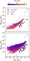 |
Fig. C.1 GCs hosting an IMBH at z = 0, compared to observed host candidates in local GCs (squares; Lützgendorf et al. 2013b) and a potential TDE (right triangle; Lin et al. 2018), for two sets of initial mass–half-mass radius conditions. The orange-edged star marks the ω Cen cluster (Häberle et al. 2024). As in Fig. 3, the dashed lines correspond to mass ratios MIMBH/Mcl = 10−1, 10−2, 10−3. The top panel shows the results from a B-POP simulation of 108 GCs, while the bottom panel shows the results from a simulation in which the same GCs have initial masses higher by 0.5 dex and half-mass radii smaller by 1 dex. |
Appendix E Bayes factor for cluster classification
In Sect. 4.2 we employed the Bayes factor to assess the relative support for two competing hypotheses regarding the nature of some GCs IMBH host candidates (Lützgendorf et al. 2013b; Kızıltan et al. 2017; Häberle et al. 2024; Bañares-Hernández et al. 2025): a globular cluster origin (HGC) or a nuclear star cluster origin (HNSC). The Bayes factor is defined as
 (E.1)
(E.1)
where
 (E.2)
(E.2)
denotes the marginal likelihood, or evidence, of the data d under hypothesis Hi. The evidence is the likelihood of the data d given the intrinsic parameters θ, averaged over their prior distribution π(θ|Hi) under hypothesis Hi. In our case, π(θ|Hi) corresponds to the two–dimensional distributions of cluster and IMBH masses obtained from Model B simulation (see Fig. 4).
Since our simulations do not provide direct access to ℒ(d, |, θ, Hi), we instead apply Bayes’ theorem to rewrite the likelihood in terms of the observed posterior probability distributions. These posteriors are approximated as Gaussians based on the values reported in Table 5 and we can denote them as p(θ | d, H0), where H0 represents the specific model assumptions adopted in each observational study. By Bayes’ theorem,
 (E.3)
(E.3)
with π(θ | H0) the prior adopted in the corresponding inference, and 𝒵(d | H0) the associated evidence.
In general, the likelihood may depend explicitly on the model assumed, i.e., ℒ (d | θ, H0) ≠ ℒ (d | θ, HGC) ≠ ℒ (d | θ, HNSC). In the present context, however, the clusters observables (e.g., velocity dispersions, luminosity profile) are governed by the same dynamical and stellar–evolutionary processes, regardless of their nature, whether globular or nuclear. Consequently, we can assume a common likelihood ℒ (d | θ) = ℒ (d | θ, H0), and attribute all model dependence to the prior π(θ|Hi). The prior π(θ|H0) entering Eq. (E.3) varies across observational studies and it is often not explicitly specified. For tractability, we approximate it as broad and uniform in both log10(Mcl) and log10(MIMBH). Hence, substituting Eq. (E.3) into Eq. (E.1), both 𝒵 (d | H0) and π(θ|H0) cancel out and the Bayes factor reduces to
 (E.4)
(E.4)
Moreover, since the priors are assumed to be broad, no relevant regions of parameter space are truncated, and the integrals can be evaluated over the full domain of π(θ|Hi). Specifically, we estimate the integrals in Eq. (E.4) using Monte Carlo summation as
 (E.5)
(E.5)
i.e., sampling θj from the host candidate properties posterior (p(θ|d, H0)) and computing the probability of such a system emerging from our simulation as a NSC or GC (π(θ|HNSC) or π(θ|HGC)).
To actually select one hypothesis over the other we would need to include in Eq. (E.4) an extra term, the so-called prior-odds of the two hypotheses, i.e., π(HNSC)/π(HGC). Including this term we would obtain
 (E.6)
(E.6)
where  is called posterior-odds. In our context, the prior odds encode the initial degree of belief about the nature of the observed hosts and can vary substantially depending on the adopted criteria. For example, one could attempt to evaluate it starting from the number of mergers the Milky Way has experienced with dwarf galaxies (i.e., the number of potential accreted nuclei) and the number of in situ GCs IMBH hosts. However, these two quantities are highly nontrivial to estimate. Moreover, the prior odds may differ for each candidate depending on properties such as metallicity spread, density profile, or galactic position.
For simplicity, in this work we focus on estimating only the Bayes factor (Eq. E.4), which measures the relative support for the globular vs. nuclear hypothesis given the data. This corresponds to evaluating the posterior odds under the assumption of equal prior probabilities for HNSC and HGC.
All Tables
Main B-POP input parameters along with the assigned value and a short description.
Bayes factor comparing a nuclear origin versus a globular origin for local IMBH host candidates.
All Figures
|
Fig. 1 Initial distribution of cluster formation redshifts. The different colors refer to different assumptions on the initial formation histories of GCs (solid lines) and NSCs (dashed lines). The initial redshift distribution of YCs is fixed in all models (gray solid line). The distributions are scaled such that the area subtended by the curve is 1. |
| In the text | |
|
Fig. 2 Left panel: initial cluster mass and half-mass radius for YCs (bottom left area), GCs (central area), and NSCs (upper right area). The cluster distributions are cut at the 99% contour. Clusters with tcc < 5 Myr lie below the dot-dashed black line; those with central density ρcl,0 > 105 M⊙ pc−3 are above the shaded dotted gray line. We also identify regions of the parameter space in which (i) a BBH binary is ejected before merging due to strong Newtonian recoils (in pink), (ii) the merger remnant is typically kicked out of the cluster due to its relativistic kick (in purple), (iii) the BBH merger time exceeds a Hubble time (in yellow). Right panel: schematic overview of a BH dynamical growth in a star cluster. The colored boxes refer to the regions highlighted in the left plot. |
| In the text | |
|
Fig. 3 Clusters hosting an IMBH at z = 0 in Model A (left panel) and Model B (right panel) compared to different classes of IMBH host candidate observations. We note that the masses reported for low-mass AGNs refer to the host galaxy mass (up to ∼ 100 times higher than the mass of the galactic nuclei). The gray dashed line shows the theoretical prediction for the initial mass of an IMBH seeded via stellar collisions (Eq. (3) in the left panel and Eq. (5) in the right panel). |
| In the text | |
|
Fig. 4 Comparison of simulated IMBH candidates in Model B with observational data. (a) Corner plot showing the GCs (purple) and NSCs (orange) clusters in our simulations hosting an IMBH at z = 0, compared to observations of potential IMBHs in Milky Way globular clusters and G1. (b) One-dimensional IMBH mass distribution, compared to estimated masses for G1 and 47 Tuc. |
| In the text | |
|
Fig. C.1 GCs hosting an IMBH at z = 0, compared to observed host candidates in local GCs (squares; Lützgendorf et al. 2013b) and a potential TDE (right triangle; Lin et al. 2018), for two sets of initial mass–half-mass radius conditions. The orange-edged star marks the ω Cen cluster (Häberle et al. 2024). As in Fig. 3, the dashed lines correspond to mass ratios MIMBH/Mcl = 10−1, 10−2, 10−3. The top panel shows the results from a B-POP simulation of 108 GCs, while the bottom panel shows the results from a simulation in which the same GCs have initial masses higher by 0.5 dex and half-mass radii smaller by 1 dex. |
| In the text | |
Current usage metrics show cumulative count of Article Views (full-text article views including HTML views, PDF and ePub downloads, according to the available data) and Abstracts Views on Vision4Press platform.
Data correspond to usage on the plateform after 2015. The current usage metrics is available 48-96 hours after online publication and is updated daily on week days.
Initial download of the metrics may take a while.