| Issue |
A&A
Volume 708, April 2026
|
|
|---|---|---|
| Article Number | A208 | |
| Number of page(s) | 11 | |
| Section | The Sun and the Heliosphere | |
| DOI | https://doi.org/10.1051/0004-6361/202557457 | |
| Published online | 08 April 2026 | |
Impact of Yaglom’s law anisotropy on the estimation of the turbulence energy transfer rate: A multipoint multiscale analysis
1
Department of Physics and Astronomy, University of Delaware, Newark, DE 19716, USA
2
Astronomical Institute of the Czech Academy of Sciences, Prague, Czechia
3
Institute of Atmospheric Physics of the Czech Academy of Sciences, Prague, Czechia
4
Lunar and Planetary Laboratory, University of Arizona, Tucson, AZ 85721, USA
5
IAPS – INAF Istituto di Astrofisica e Planetologia Spaziali, 00133 Roma, Italy
6
IRF Swedish Institute of Space Physics, Uppsala, Sweden
7
Laboratoire de Physique des Plasmas, CNRS, 91128 Palaiseau, France
★ Corresponding author: This email address is being protected from spambots. You need JavaScript enabled to view it.
Received:
28
September
2025
Accepted:
30
January
2026
Abstract
Context. Spectral anisotropy is a ubiquitous characteristic of turbulence in magnetized space plasma environments, as it occurs spontaneously due to the effect of a background magnetic field. This anisotropy significantly affects the turbulent energy cascade and modifies the scale-to-scale balance between different terms in the von Kármán-Howarth equation.
Aims. We investigate the effect of the induced lag-space anisotropy on the determination of the scale-dependent energy transfer rate.
Methods. We compared traditional single-spacecraft and novel multispacecraft approaches using hybrid particle-in-cell simulations and in situ observations from the Magnetospheric Multiscale (MMS) mission in the Earth’s magnetosheath.
Results. We show that the isotropy assumption, which is required for single-spacecraft measurements, leads to inaccuracies in the estimation of the turbulent cascade rate. On the other hand, the novel lag-polyhedra derivative ensemble method, which is specifically designed for the next generation of multipoint multiscale missions such as HelioSwarm and Plasma Observatory, can capture the anisotropy of the turbulent cascade.
Conclusions. These findings are used to interpret observations from the MMS mission in the Earth’s magnetosheath. They highlight the importance of accounting for anisotropy in space plasma diagnostics.
Key words: magnetohydrodynamics (MHD) / plasmas / turbulence / solar wind
© The Authors 2026
 Open Access article, published by EDP Sciences, under the terms of the Creative Commons Attribution License (https://creativecommons.org/licenses/by/4.0), which permits unrestricted use, distribution, and reproduction in any medium, provided the original work is properly cited.
This article is published in open access under the Subscribe to Open model. This email address is being protected from spambots. You need JavaScript enabled to view it. to support open access publication.
1. Introduction
Turbulence is a state of fluid or plasma flow that is characterized by seemingly random and chaotic fluctuations across a vast spectrum of spatial and temporal scales. It is a fundamental characteristic of diverse astrophysical and space plasma environments. In systems such as the solar wind, planetary magnetospheres, and the interstellar medium, turbulence plays a pivotal role in shaping physical properties and evolution (Bruno & Carbone 2005; Matthaeus & Velli 2011). The nonlinear interactions inherent to turbulent flows cause the continuous transfer of energy from large-scale driving motions that feed energy into the system to progressively smaller scales at which this energy is ultimately dissipated (Batchelor 1953; Tennekes & Lumley 1972; Frisch 1995; Pope 2000). Understanding the precise mechanisms involved and the rate at which this turbulent energy cascade proceeds is paramount for comprehending a wide range of phenomena, including heating, acceleration of high-energy particles, and the overall transport processes that govern the structure and dynamics of space plasmas (Usmanov et al. 2018; Pezzi et al. 2021).
Kolmogorov’s theory of homogeneous and isotropic turbulence (Kolmogorov 1941b,a) defines the notion of an energy cascade, a scale-by-scale transfer of kinetic energy from larger to smaller eddies through nonlinear interactions. In a statistically steady state, the net rate at which energy is transferred down the scales, denoted by ϵ, is equal to the rate at which energy is provided to the system at the largest scales and dissipated at the smallest. Within the inertial range, the spectrum of scales between the dissipative and the injection scales, the energy cascades at a constant rate ϵ. A consequence of this assumption is the well-known prediction for the omnidirectional power spectral density E(k)∝k−5/3, where k ∝ l−1 is the wavenumber associated with length l.
A fundamental theory for investigating the statistical properties of energy evolution in turbulent flows is the von Kármán-Howarth (vKH) equation (de Karman & Howarth 1938), derived for homogeneous isotropic incompressible hydrodynamics (HD). This equation provides a dynamical relation for the evolution of the energy in time and across scales involving second- and third-order correlations of the velocity field. The third-order correlations are intrinsically linked to the nonlinear transfer of energy between different scales in the turbulent cascade. This result was also obtained by Kolmogorov (1941a) as the famous 4/5 law that links third-order correlations to the mean energy dissipation rate ϵ. This relation offers a direct pathway to experimentally determining the energy cascade rate in HD turbulence through measurements of the third-order velocity structure function (Frisch 1995).
Later theoretical development by Politano & Pouquet (1998a,b) extended this earlier work from isotropic homogeneous incompressible HD to homogeneous incompressible magnetohydrodynamics (MHD). In the case of space and astrophysical plasma, the common presence of a background magnetic field often induces a preferred direction, leading to distinct behaviors in the parallel and perpendicular directions.
Observational investigations of turbulence in space plasma rely critically on in situ measurements. Single-spacecraft missions provide data at a single point in space, facing inherent limitations when it comes to resolving the multiscale spatial structure of turbulence. This includes limitations in directly evaluating the third-order correlation tensor or structure functions, which is essential for characterizing the energy cascade.
To circumvent this limitation, the Taylor hypothesis, or frozen-in flow approximation, is frequently invoked (Taylor 1938; Jokipii 1973; Fredricks & Coroniti 1976). The assumption is that the temporal variations observed by a stationary spacecraft are primarily due to the advection of preexisting spatial structures past the spacecraft by a mean flow, such as the solar wind, rather than temporal change in the flow frame. This requires that the dynamical evolution of turbulence is slower than the observational time. Under this assumption, temporal fluctuations can be converted into spatial scales using the mean flow velocity. However, the validity of the Taylor hypothesis can be compromised in various situations, including when the turbulent fluctuations have significant temporal evolution on the timescale of advection or when the amplitude of the fluctuations is comparable to or higher than the mean flow speed. These deviations can lead to inaccuracies in the inferred spatial scales and consequently affect the estimation of quantities related to the energy cascade, as recently investigated using Parker Solar Probe (PSP; Fox et al. 2016) observations (Klein et al. 2015; Bourouaine & Perez 2018; Chhiber et al. 2019; Perez et al. 2021).
Despite the limitations imposed by the assumptions of isotropy and applicability of Taylor’s hypothesis, these are necessary simplifications when only single-spacecraft measurements are available. Moreover, another necessary simplification is the restriction of the analysis to the inertial range, which is well separated from energy injection and dissipation scales. In the latter case, the vKH equation (Eq. 1 below) reduces to the Yaglom- or third-order law (Eq. 2). Upon enforcing the isotropy condition, this is further simplified to the well-known Politano & Pouquet (PP) law (Eq. 3). This equation is largely present in the literature and provided the analytical framework for the observations of an inertial range using third-order moments in space (MacBride et al. 2005; Sorriso-Valvo et al. 2007; Stawarz et al. 2009; Marino et al. 2011; Hadid et al. 2017). Additional theoretical efforts involved the development of the vKH equation for compressible MHD (Carbone et al. 2009; Andrés & Sahraoui 2017; Hellinger et al. 2021), and in the presence of Hall effects (Galtier 2008; Hellinger et al. 2018; Ferrand et al. 2019; for a review, see Marino & Sorriso-Valvo 2023).
The advent of multispacecraft missions, such as Cluster (Balogh et al. 1997), Time History of Events and Macroscale Interactions during Substorms (THEMIS; Angelopoulos 2008), Acceleration, Reconnection, Turbulence and Electrodynamics of the Moon’s Interaction with the Sun (ARTEMIS; Angelopoulos 2011, and Magnetospheric Multiscale (MMS; Burch et al. 2016), has revolutionized the study of space plasma turbulence, allowing for simultaneous multipoint measurements. This allowed for the direct estimation of spatial gradients (using, e.g., curlometer-like techniques, Dunlop et al. 1988; Paschmann & Daly 1998, Chap. 16) and fundamental quantities such as two-point correlation functions (Matthaeus et al. 2005), structure functions, and higher-order statistics without relying on Taylor’s hypothesis (Isaacs et al. 2015; Chasapis et al. 2017; Chhiber et al. 2018; Bandyopadhyay et al. 2018a; Roberts et al. 2022).
Despite the significant advancements enabled by multispacecraft missions, these observations are essentially limited to a single scale at a time, nullifying the possibility of investigating the inherent multiscale nature of space plasma turbulence. Even with multispacecraft missions, the evaluation of the energy transfer rate requires invoking the frozen-in approximation (Bandyopadhyay et al. 2018b; Hadid et al. 2018; Andrés et al. 2019; Quijia et al. 2021). Moreover, the anisotropy induced by the background magnetic field promoted the development of alternative techniques to measure the energy cascade rate employing directional averages (Osman et al. 2011; Bandyopadhyay et al. 2018b) or multicomponent models (MacBride et al. 2008; Stawarz et al. 2009; Andrés et al. 2022).
These limitations will be overcome with the advent of the next generation of multipoint multiscale missions. The HelioSwarm (HS; Klein et al. 2023) and Plasma Observatory (PO; Marcucci & Retinò 2024) missions feature nine and seven spacecraft, respectively, that will sample turbulence in a variety of near-Earth plasma environments, as illustrated in Fig. 1. Their configurations allow for the first time the evaluation of the vKH equation without invoking the isotropy condition or the frozen-in approximation.
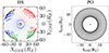 |
Fig. 1. Orbital plot showing the precession of the HS (left) and PO (right) observatory trajectories around the Earth (⨁ for HS and blue dot for PO), with regions of interest highlighted in blue (magnetosphere), red (solar wind), and green (foreshock) for HS. The thick lines in the HS plot indicate hours with ideal 3D multiscale coverage. The specific configuration we analyzed is marked with a black (red) dot for HS (PO). At this scale, it is not possible to distinguish individual spacecraft trajectories. |
To effectively address the increasing complexity of future observations and optimize the scientific return of current and upcoming space missions, the development of innovative techniques is essential (Klein et al. 2024; Pecora et al. 2024; Broeren et al. 2024; Dunlop et al. 2024; Shen et al. 2025). The lag-polyhedra derivative ensemble (LPDE) technique (Pecora et al. 2023a) represents a step forward in this direction. Initially applied to MMS data (Pecora et al. 2023b; Pecora 2024), this technique provides the numerous estimations needed to achieve convergence of the energy transfer rate. In the following sections, we broaden the application of the LPDE technique, including both numerical simulations and observational data, and we compare the findings obtained under the assumption of isotropy with those where this assumption is relaxed.
In Sect. 2 we present the theoretical framework of the vKH equation, and Sect. 3 describes the numerical simulations that are employed and the numerical results. In Sect. 4 we show the results obtained using MMS data. The results are commented on and discussed in the final section.
2. Theoretical framework
The vKH equation, initially obtained for HD (de Karman & Howarth 1938), describes the energy evolution in time and across scales in a homogeneous turbulent flow. Later extended to magnetized flows in the context of MHD (Politano & Pouquet 1998a,b), the equation reads
 (1)
(1)
and is written in terms of increments of the Elsässer fields z± = v ± b, namely δz±(ℓ) = z±(x)−z±(x + ℓ) with vector separation (lag) ℓ. Here, v and b are the velocity and the magnetic field fluctuations, the latter is in Alfvén units, normalized to  for proton number density np and mass mp, and ν is the kinematic viscosity. Derivatives ∇[ℓ are in lag (or increment) space, and
  is the average energy transfer rate.
The time-dependent term in Eq. (1) is significant at large scales but remains inaccessible to spacecraft observations because it requires the instrument to track a parcel of plasma in a Lagrangian fashion. The nonlinear term incorporates the mixed third-order structure function and is associated with the energy cascade within the inertial range. Last, the dissipative term, which generally becomes prominent at small scales, presents considerable theoretical difficulties in establishing the nature of the dissipative function in a noncollisional plasma (see Pezzi et al. 2021; Yang et al. 2022, 2024; Adhikari et al. 2025). The vKH equation states that at all times and scales, the sum of these three terms is always proportional to the energy cascade rate.
When the system attains distinct scale separation or, equivalently, the Reynolds number is sufficiently high1, each of these terms becomes dominant within its corresponding range of scales, where the other two terms contribute negligibly. For instance, in such cases, within the inertial range, the vKH Eq. (1) simplifies to the so-called Yaglom or third-order law,
 (2)
(2)
where the argument of the lag-space divergence is the Yaglom flux Y± = ⟨δz∓|δz±|2⟩. Equation (2) is a fundamental framework for the analysis of space plasma, as it is currently the only term of Eq. (1) that can be directly investigated using spacecraft observations.
Equation (2) requires a constellation of at least four noncoplanar spacecraft to be solved. Currently, MMS is the only mission that provides the necessary measurements (density, velocity, and magnetic field) on all four spacecraft to solve Eq. (2). When only single-spacecraft measurements are available, Eq. (2) can be simplified (Politano & Pouquet 1998a,b), under the assumption of isotropy, to
 (3)
(3)
where Y± now represents the projection of the Yaglom flux along the direction  , with
  denoting the direction of the plasma (solar wind) flow and τ the temporal increments in the observational time series. This clearly requires not only an assumption of isotropy, but also the application of Taylor’s hypothesis.
The assumption of isotropy of Yaglom flux Y± that leads to use of Eq. (3) can result in inaccurate estimations of the energy cascade rate, while Taylor’s hypothesis introduces challenges related to space-time decorrelation (Matthaeus et al. 2010, 2016; Pecora et al. 2025b). As we show below, both of these issues are resolved when a multipoint multiscale constellation of spacecraft is available2.
Of the three terms on the left-hand side of Eq. (1), only the nonlinear term can be measured by spacecraft constellations. Therefore, our analysis is restricted to this term. To simplify the notation, we refer to the total cascade rate (ϵ+ + ϵ−)/2 derived from Eq. (2) below as ϵY or, more simply, ϵ.
3. Numerical analysis
3.1. Hybrid PIC simulations
The 3D hybrid particle-in-cell (PIC) simulations, employing kinetic ions and fluid massless electrons, were conducted within a cubic domain discretized with 5123 grid points. The spatial resolution was uniform across all dimensions, Δx = di/8, where di is the ion inertial length, resulting in a total physical length of 64di for each side of the simulation box. The ion velocity distribution function was initialized as isotropic, with a plasma beta βi = 0.5 (the ratio of magnetic to kinetic pressures). Fluid electrons, described by an isothermal equation of state with βe = βi, provide charge neutrality. The mean magnetic field B0 was oriented in the z direction.
These simulations were performed using the code Camelia (Franci et al. 2015, 2018a,b), and this analysis used the simulation results detailed in Hellinger et al. (2024). The simulation models decaying turbulence, characterized by initial fluctuations at relatively large scales that evolve into a turbulent cascade, which can be analyzed using the vKH equation. The initial cross helicity was set to zero and remained approximately zero throughout the simulation. Using the simulation fields, we computed solutions to the scale-dependent Yaglom law, which serves as a reference solution for the comparison with virtual spacecraft estimates. Using the simulation values at the grid points, we solved Eq. 2 exactly (up to the discretization error of finite difference methods). Throughout the paper, this is the solution against which single- and multispacecraft estimates are compared to assess their accuracy.
3.2. Virtual spacecraft configurations
3.2.1. Single spacecraft
To investigate the effect of magnetic field-induced anisotropy on single-point estimations of the cascade rate, we simulated single-spacecraft trajectories at various angles relative to the background magnetic field. While not directly reproducible with observational data, these trajectories provide a valuable numerical framework for assessing the limitations of the isotropy assumption.
Single-spacecraft measurements inherently do not permit the calculation of 3D spatial derivatives, even with the aid of the Taylor hypothesis, thus necessitating an assumption of isotropy to estimate the cascade rate using the PP law (Eq. 3). This simplification enables the estimation of the nonlinear energy transfer rate as ϵ = −3Y/4ℓ, where Y is the longitudinal component of the Yaglom flux (representing either Y+ or Y− projected along the plasma flow direction). Although this approach is widely adopted in space plasma analysis due to its reliance on single-point measurements, the inherent anisotropy induced by the background magnetic field, usually present in interplanetary space, can lead to inaccuracies. Furthermore, probing the relevant scales often requires the frozen-in flow hypothesis, which can introduce its own complexities related to space-time correlations (Matthaeus et al. 2016).
We generated virtual spacecraft trajectories at angles ranging from 9° to 69° with respect to the mean magnetic field. Magnetic field and plasma moments (density and velocity) were interpolated to the position of the virtual spacecraft within the simulation domain. This procedure allowed us to compute the longitudinal Yaglom flux and subsequently estimate the energy cascade rate using the standard isotropic (PP) formulation in Eq. (3).
3.2.2. Multispacecraft
With the availability of multiple spacecraft, the assumption of isotropy for solving the divergence term in Eq. (2) becomes unnecessary. Instead, we can employ curlometer-like techniques (Dunlop et al. 1988). These methods are not applied to the physical spacecraft constellation directly, but to virtual tetrahedra assembled within the lag space defined by the separations between spacecraft (Pecora et al. 2023a).
The method proceeds as follows: for each pair of spacecraft separated by a vector lag ℓ, a corresponding value of the Yaglom flux, Y(ℓ) (we dropped the superscript ± as the procedure always involves computing Y± to then obtain the average cascade rate, as discussed above), was computed from the increments of the Elsässer fields. As noted in Pecora et al. (2023b), the third-order moment exhibits odd symmetry with respect to its vector lag, that is, Y(−ℓ) = − Y(ℓ), which allows for the doubling of data points in lag space.
Now, any combination of four values of Yaglom fluxes delineates a tetrahedron in lag space with the values of Y measured at the vertices. The number of possible tetrahedra scales combinatorially as C2n4, where n is the number of available Y measurements before symmetrization by exploiting the odd symmetry of Y. This symmetrization generates some redundant solutions (the tetrahedron obtained from any four values of Y is necessarily identical to that obtained from the reflections of those four points), as well as some physically meaningless solutions corresponding to zero lag (obtained from tetrahedra formed by any two values of Y and their reflection) that are discarded. This is taken into account by correcting C2n4 to  . This is the number of unique nonredundant tetrahedra, a number significantly larger than Cn4 (a four-point constellation such as MMS provides the minimum possible n = 6). This abundance of tetrahedra yields numerous independent solutions for the divergence in Eq. (2), thereby providing robust statistical validation of the final result. The exploitation of this large number of tetrahedra (which can be extended to more general polyhedra) is the core of the LPDE technique, which has been used to solve Yaglom’s law in simulations (Pecora et al. 2023a), and, in conjunction with the symmetry properties of the third-order moment, MMS data (Pecora et al. 2023b).
For relevance to upcoming multipoint multiscale spacecraft missions, we used realistic representative configurations for HS (nine spacecraft; Klein et al. 2023; Niehof et al. 2024 and Plasma Observatory (7 spacecraft, Retinò et al. 2022; Marcucci & Retinò 2024). The planned orbital trajectories for HS and PO, along with the location of the used spacecraft configurations, are presented in Fig. 1. These orbits are displayed in the XY plane of the Geocentric Solar Ecliptic (GSE) coordinate system, in which the Earth is positioned at the origin (0, 0), the X-axis is along the Earth-Sun direction, Y is in the ecliptic plane pointing toward dusk (opposing planetary motion), and Z is parallel to the ecliptic pole.
The projections of the individual spacecraft positions onto the three orthogonal planes of the GSE system are shown in Fig. 2. For HS, positions are expressed relative to the central hub spacecraft. For PO, positions are measured relative to the constellation barycenter.
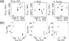 |
Fig. 2. HS and PO relative position of the spacecraft within each observatory. For HS, the central hub is displayed in red, and positions are measured relative to it. For PO, positions are measured relative to the barycenter. |
Finally, Fig. 3 illustrates the magnitudes of available interspacecraft separations (lags), derived from all possible spacecraft pair combinations (36 for HS and 21 for PO). These lags are displayed in the radial-tangential-normal coordinate system for HS and in the GSE coordinate system for PO. For HS, the panels incorporate three color bands delineating the kinetic, transition, and MHD ranges of plasma turbulence using solar wind characteristic scales. The kinetic regime is probed by spacecraft separations below 100 km (comparable to the typical ion inertial length di, Verscharen et al. 2019), while MHD scales are accessed with separations exceeding 1200 km. Within the magnetosphere, these characteristic scales are smaller. For PO, a shaded region highlights lags smaller than 50 km, which corresponds to the kinetic range based on nominal values of the ion inertial length in the magnetosheath, while 1000 km separations would encompass nearly the entire inertial range, approaching the correlation scale (Stawarz et al. 2022; Pecora et al. 2025a).
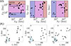 |
Fig. 3. HS and PO baseline magnitudes. For HS, kinetic, transition, and MHD ranges are indicated with color bands. For PO, only the kinetic range below 50 km is indicated with a shaded area. |
For our study, the virtual spacecraft constellations sampled the simulation domain at a fixed angle relative to the background magnetic field. Virtual multispacecraft configurations were tested across a range of angles relative to the mean magnetic field, but no substantial alterations to the results were observed. This is expected because we measured a scalar quantity. Interspacecraft separations were maintained at constant values. This emulates the observation of a data stream spanning multiple correlation lengths, ensuring convergence of higher-order statistics while being sufficiently short to prevent significant changes in the relative spacecraft positioning during the observation period. For HS, the observatory has a change of ∼1% on average in baseline separations between s/c over an hour near apogee; the correlation time at 1 au is about 45 minutes (Ruiz et al. 2014; Isaacs et al. 2015; Cuesta et al. 2022).
The analyses below were conducted twice: first using a spacecraft configuration rescaled within the simulation domain to focus on shorter-scale ranges. In the second instance, the scaling factor was chosen so that the constellations could encompass a substantial fraction of the inertial range, defined within the simulation as the region in which the nonlinear term of the vKH equation plateaus.
These two approaches were tuned for the investigation of several numerical and realistic aspects. Short separations are anticipated to yield more accurate derivative estimates. Additionally, small configurations sample a scale range comparable to that expected for the real mission in the solar wind. This strategy is necessary as simulations cannot achieve the scale separation of real systems. Conversely, the larger configuration allows for assessing the stability of the solution to Eq. (2) under conditions of potentially less accurate derivatives, while also covering a scale range similar to that encompassed in the magnetosphere.
As detailed above, with nine spacecraft, 36 independent Yaglom flux values can be obtained from all spacecraft pairs, which can be combined to form C436 = 58 905 tetrahedra. However, by exploiting the odd symmetry of Y, the number of independent lag-space tetrahedra (and consequently, the solutions to Eq. 2) can be significantly increased to  . The factor of 1/2 ensures that only unique solutions are counted, avoiding consideration of solutions obtained from a set of four points and their reflections about the origin, which yield the same result for geometrical reasons. Furthermore, the correction C236 accounts for tetrahedra centered exactly at the origin, which would assign the solution to zero lag, which is difficult to interpret physically. We recall that in the standard curlometer technique, the solutions for the derivatives are attributed to the lag corresponding to the barycenter of each tetrahedron. Despite these corrections aimed at excluding redundant and physically ambiguous solutions, this approach yields an increase of almost an order of magnitude in the number of available solutions with nine spacecraft. In the case of PO, the number of total solutions is
  .
.
3.3. Simulation results
The comparison of the different techniques detailed in the previous sections used to solve Yaglom’s law is shown in Fig. 4. The benchmark for evaluating the accuracy of these methods is the direct solution of Eq. (2), obtained via finite difference methods applied to the simulation grid, depicted by a red line with plus symbols and associated error bars. These symbols represent locally averaged values within bins, with error bars indicating the dispersion around their respective means. It is observed that the spread of solutions increases at larger lags, a consequence of the larger separations used in the finite difference derivative calculations at these scales. It is important to note that these results are presented as a function of lag magnitude, averaged over different directions. Solutions expressed as a function of vector lag separations are provided subsequently. As described earlier, the energy cascade rate, calculated using Yaglom’s law, is expected to exhibit a plateau at intermediate scales within the inertial range. Its contribution diminishes at small scales, where the dissipative term of the vKH equation dominates, and at large scales, where the time-dependent term becomes dominant.
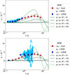 |
Fig. 4. Scale-dependent energy cascade rate from Yaglom’s law using different methods. Grid-computed exact solution (red plus). We show single-s/c PP estimates at varying angles to B0 (green lines). We also show LPDE multi-s/c solutions (cyan cross) and the LPDE average (large blue cross), and the error bars indicate the standard deviation. Top: LPDE on smaller-scale HS. Bottom: LPDE on larger-scale HS. |
For comparison, the subsequent analysis examined virtual single spacecraft crossings of the simulation domain at various angles relative to the mean magnetic field. Under the assumption of isotropy, this approach yields the solution of Eq. (3), depicted by the solid green lines in the figure, corresponding to angles ranging from 9° to 69°. In an isotropic system, with no preferred direction, these curves are expected to overlap. This was demonstrated by Jiang et al. (2023), who found precise overlap of the cascade rates measured using the PP law at various angles in MHD simulations with no mean field. However, the presence of a background magnetic field introduces anisotropy, leading to substantial deviations in these estimates. These deviations are attributed to the anisotropic nature of the turbulent cascade, which is less efficient in the direction parallel to the mean field, while it generates smaller scales in the perpendicular plane more efficiently. These findings corroborate previous theoretical and numerical studies (Shebalin et al. 1983; Matthaeus et al. 1996; Oughton & Matthaeus 2005; Howes 2008). Trajectories more closely aligned with the mean magnetic field show, indeed, suppressed values for the energy transfer rate obtained from the nonlinear term in the vKH equation. Conversely, an overestimation of this quantity is observed in the perpendicular direction (Verdini et al. 2015; Jiang et al. 2023).
In addition to significant variations in the magnitude of the estimated energy transfer rate, the relatively flat region, indicative of the inertial range, also exhibits a shift across scales. This is particularly relevant when the third-order law is used to define the extent of the inertial range. The plateau observed in Yaglom’s law gives a more robust detection of the inertial range as it represents a higher-order moment compared to, for example, the power spectral density, which is more commonly used to detect the inertial range (see, e.g., Bruno & Carbone (2005), Marino et al. (2012).) Nevertheless, the current analysis reveals a systematic and nontrivial misalignment of the inertial range when determined using single-spacecraft measurements along different directions in an anisotropic medium.
The final set of solutions was derived using LPDE. Individual solutions are represented by small, light blue crosses, with their binned average indicated by a larger blue cross and associated error bars denoting the standard deviation within each bin. We used the signed value of the cascade rate to compute averages. For each lag-space tetrahedron used in solving Yaglom’s law, we computed the elongation (E) and planarity (P) defined as  and
and  . Here, λs represents the eigenvalues of the volumetric tensor
  , where ℓαi is the ith component of vertex α, and K = 4. The term ℓbj = ⟨ℓαj⟩α denotes the lag-space position of the barycenter of the considered tetrahedron, with its vertices labeled by α (Paschmann & Daly 1998; Pecora et al. 2023b; Pecora 2024).
These parameters were used to assess the regularity of a tetrahedron. By measuring the norm  , we selected more robust solutions by restricting the analysis to tetrahedra with χ < 0.6, which correspond to uncertainties smaller than 20% (see page 408 of Paschmann & Daly 1998). In the present analysis, we included tetrahedra with a slightly relaxed threshold of χ ≤ 0.7. This specific threshold was determined through a convergence study. Starting from a more conservative value of χ = 0.4, we progressively increased the threshold as long as the average values per bin remained constant. For thresholds χ > 0.7, this condition was no longer met. This approach allowed us to retain the maximum number of solutions for statistical robustness while ensuring that the average values remained stable. Furthermore, we only included tetrahedra with a volume smaller than that of a cube of side ∼12Δx = 1.5di. It is important to note that this volume refers to the space enclosed by the tetrahedron itself and is distinct from the lag-space position ℓ of the barycenter to which the solution is assigned.
The two panels in Fig. 4 present the same finite difference (red) and isotropic (green) solutions, but distinct LPDE solutions using two variations of HS trajectories. These clouds of solutions were obtained by rescaling the multispacecraft constellation to encompass smaller distances in the first panel and larger distances in the second. In the first case, Δx in the simulation corresponds to a spatial separation of 400 km, whereas in the second, it corresponds to 50 km. These rescaling factors were chosen to minimize overlap between the two sets of points, thereby avoiding redundant analyses, while encompassing the scales of interest of the two missions (di ∼ 100 km in the solar wind, and ∼50 km in the magnetosheath). In all configurations, the averaged LPDE solution demonstrates remarkable agreement with the benchmark solution obtained directly from the simulation grid.
Intuitively, increased spacecraft separations lead to larger uncertainties, reflected by a broader spread of solutions. However, as shown in Fig. 5, the ratio of the bin-averaged ϵ to the standard deviation about the mean σ is relatively stable, remaining below 40% (except for the last point of the large configuration). This stability is observed across the two different spacecraft configurations, independent of their overall scale, again confirming the importance of a large number of estimates and the robustness of LPDE.
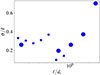 |
Fig. 5. Relative standard deviation of LPDE measurements (bin average energy transfer rate |

This comparative analysis of these distinct methods confirms that assuming isotropy can lead to substantial inaccuracies in estimating the energy transfer rate in the presence of a background magnetic field. Multipoint multiscale approaches are crucial for obtaining reliable measurements of this fundamental quantity in space plasma.
The effect of spectral anisotropy is distinctly evident in the Yaglom flux vectors. Analogous to the Poynting vector, the orientation of the Yaglom flux identifies the direction of the energy flow across scales. In an isotropic medium, energy transfer from large to small scales occurs without a preferred direction, leading to Yaglom flux vectors that converge uniformly (isotropically) toward the origin of the lag space (see Fig. 8 in Adhikari et al. 2023). However, when the system is anisotropic, deviations from this behavior are expected. In our simulations, we observe such a deviation as depicted by the Yaglom flux vectors projected onto the parallel-perpendicular increment plane in Fig. 6a. The flux vectors confirm that energy is transferred from large scales (long lags) toward the origin of the lag space, where it eventually dissipates. The orientation of these vectors is consistent with a turbulent cascade within an anisotropic medium, as observed in previous rotating HD experiments (Lamriben et al. 2011), MHD numerical studies (Verdini et al. 2015), and MMS observations in the magnetosheath (Pecora et al. 2023b). Figure 6b presents the joint distribution of the energy transfer rate in the parallel-perpendicular increment plane. The distribution is distinctly elongated along the parallel direction, signifying that the turbulent energy transfer rate is active at perpendicular scales smaller than in the parallel direction, where it is more suppressed.
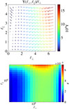 |
Fig. 6. (Top) Yaglom flux vector projected in the parallel-perpendicular increment plane. The arrows illustrate the transport of energy from large to small scales, consistent with a turbulent cascade that is predominantly active in the perpendicular direction. The arrow lengths are normalized by ℓ⊥ for visualization purposes, and the color reflects the non-normalized magnitude. (Bottom) Divergence of the Yaglom flux vector in the parallel-perpendicular increment plane. The elongated feature along the parallel direction is indicative of turbulent energy transfer more active in the perpendicular direction. |
The multiscale spacecraft configurations offer a valuable opportunity to investigate the anisotropy of the turbulent cascade by providing numerous estimates across various scales. LPDE solutions obtained from Eq. (2) provide a scale-dependent energy transfer rate, ϵ(ℓ), for each vector separation ℓ within the increment space. Under the assumption of gyrotropy within the plane perpendicular to the background magnetic field, this quantity can be represented as ϵ(ℓ⊥, ℓ∥), as depicted in Fig. 7.
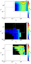 |
Fig. 7. Anisotropic energy cascade rate ϵ(ℓ⊥, ℓ∥) in the parallel-perpendicular increment plane (assuming gyrotropy). Top: Full simulation grid solution (benchmark). Middle: HS with smaller separations (kinetic scales). Bottom: HS with larger separations (inertial scales). Even with limited coverage, HS recovers the scale-dependent anisotropic trend. Different configurations cover different portions of the increment space. The coverage on the simulation grid and HS are delimited with solid and dashed gray boxes, respectively. The black lines are isocontours of the energy transfer rate. |
All three panels of Fig. 7 span the same domain of the parallel-perpendicular increment plane. The three grey boxes delimit the portion of the plane covered by the simulation grid (solid box), the small and large spacecraft configurations (dashed boxes at smaller and larger scales, respectively). In separate panels, each smaller box is filled with a color map of the measured energy transfer rate. In the top panel of Fig. 7, we present the solution to Eq. (2), directly computed from the simulation grid points, as in Fig. 6. The contours of constant ϵ are overlaid.
While spacecraft coverage in lag space is inevitably more restricted than the full simulation grid and samples some separations smaller than the grid cell, the fundamental anisotropic trend of the nonlinear energy transfer rate is preserved. Notably, in the smaller configuration (Fig. 7 center), the elongation in the parallel direction is clear. For the small and large (Fig. 7 bottom) configurations, the scale-dependent energy cascade rate consistently increases with larger separations. This confirms that multipoint multiscale measurements not only enable the accurate determination of the scale-dependent energy transfer rate, but also provide insights into its anisotropic nature, or equivalently, into the anisotropic balance of terms in the vKH equation.
Results from the Plasma Observatory 7-spacecraft configuration yield highly similar outcomes. This reinforces the feasibility of conducting comparable analyses in distinct plasma environments with different constellations of spacecraft and suggests that comprehensive estimates of the energy transfer rate can be obtained in the solar wind using HS and in the magnetosheath with PO, thereby providing a more complete understanding of energy dynamics in these space plasmas.
4. MMS
In this section, we analyze five magnetosheath intervals observed by the MMS mission that were previously examined in Pecora (2024). To compute Elsässer variables, we used magnetic field, velocity, and density data. The magnetic field measurements were acquired from the Fluxgate Magnetometer (FGM; Russell et al. 2016), and the plasma properties were obtained from the Fast Plasma Investigation (FPI; Pollock et al. 2016). These intervals feature burst-mode data in which the magnetic field is sampled at 128 Hz and the plasma moments at 150 ms. To compute composite quantities, such as the Elsässer fields, magnetic field data were down-sampled to match the plasma measurement cadence. Unlike the simulation analysis, no direct benchmark is available for these observational data. Consequently, the interpretation of the MMS results relies on insights derived from the simulation. Analogous to the simulation analyses, we computed Yaglom’s law using the PP formulation in Eq. (3) and the complete formulation in Eq. (2), solved via LPDE.
The estimates of the energy transfer rate, obtained using the PP formulation of Yaglom’s law, are presented in Fig. 8. As frequently seen in prior observational studies (MacBride et al. 2008; Stawarz et al. 2009; Carbone et al. 2009), these estimates often exhibit an alternating pattern of positive and negative values. This oscillatory behavior complicates the physical interpretation of the energy cascade rate. A common approach to mitigating this issue involves taking the absolute value of the estimated cascade rate (Hadid et al. 2017, 2018; Bandyopadhyay et al. 2018b; Andrés et al. 2019). Negative values of the energy transfer rate have also been associated with inverse energy transfer in some contexts (Marino et al. 2008; Marino & Sorriso-Valvo 2023; Marino & Xie 2025).
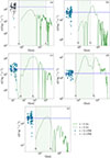 |
Fig. 8. Estimates of Eq. (2) (filled blue circles for positive ϵ, and white circles for negative ϵ) using LPDE. The horizontal line is the average value (solid for positive, dashed for negative). The isotropic estimate from Eq. (3) (solid green lines for positive values, and dashed lines for negative values). The ion inertial length di and the correlation length λc are indicated in each panel. The different estimates of the isotropic cascade rate were obtained within the shaded green areas between 1.2di and 0.8λc. Panels (a)-(e) correspond to intervals I-V, respectively. |
Conversely, as tested with numerical simulations, LPDE yields more robust estimates. This enhanced robustness is due to the large number of solutions available within each interval and to the absence of any symmetry assumptions. As previously discussed, filtering solutions based on the quality factor of tetrahedra reduces the total number of available estimates. However, with MMS, approximately 100 data points are available per interval (as reported in Table 1). It is important to note that contamination from opposite-sign solutions is minimal to nonexistent, thereby affirming the reliability of this approach. Positive solutions are represented by filled blue circles, while negative estimates are indicated by white circles. Furthermore, the magnitude variability of the LPDE solutions is generally low and is typically confined within a factor of 3, with only a few isolated outliers.
Parameters of the five analyzed MMS intervals.
The observed lack of overalp in scale between the LPDE and PP estimates can be attributed to the combined effects of MMS separation distances and instrumental resolution. The spatial lag derived from the Taylor hypothesis for the PP formulation, assuming an average solar wind speed of 200 km/s in the magnetosheath (Pecora et al. 2025a), is approximately 30 km, given the 150 ms resolution of the plasma instrument. This separation is larger than the MMS constellation scale. In intervals III and IV (Fig. 8 panels c and d), a partial overlap is observed, which is attributable to a slower solar wind speed during these periods (see Table 1 for MMS minimum and maximum separations during these intervals).
The application of Yaglom’s law for determining the total energy cascade rate is rigorously valid only within the inertial range where contributions from time-dependent and dissipative terms in the vKH equation become negligible. As previously described, the scale dependence of the nonlinear term is expected to exhibit an increasing trend at scales larger than the ion inertial length di, followed by a relatively flat region within the inertial range, and subsequently, a decreasing trend at scales exceeding the correlation length λc. Our numerical analyses employing multiscale spacecraft configurations successfully reconstructed the anticipated scale-dependent profile of the nonlinear term with a plateau region when spacecraft separations were sufficiently large to fall within the inertial range. In this case, a reliable estimation of the total cascade rate is possible.
The measurements by MMS are provided at a single scale, which precludes the direct reconstruction of the scale-dependent behavior of the energy transfer rate without employing Taylor’s hypothesis. Furthermore, the spatial separations in MMS data are frequently smaller than di. Consequently, the transfer rates obtained using LPDE for MMS data correspond to the increasing ramp of the scale-dependent curve and should therefore not be interpreted as the total energy cascade rate. Instead, these values represent the contribution to the total transfer rate from the nonlinear term at these specific scales. To obtain the total energy cascade rate, the contribution from the dissipative term should be added to these estimates. However, this poses theoretical and technical challenges that are beyond the scope of the present analysis.
An extension to a sufficiently broad range of scales to capture the entire scale-dependent trend is only possible by applying Taylor’s hypothesis, albeit under the assumption of isotropy, the implications of which warrant further discussion. The anticipated scale-dependent behavior is loosely observed in the MMS intervals when the PP formulation is applied. Only interval III unequivocally exhibits a more distinct plateau centered around the correlation length. Interestingly, all intervals provide a negative energy transfer rate when they are analyzed with the isotropic formulation, contrasting with LPDE estimates, which return a negative cascade rate exclusively for interval I. The isotropic formulation also displays the commonly observed (but absent in simulations) alternating pattern of negative and positive values, although these particular intervals show a predominance of negative values. A comprehensive statistical analysis is necessary to further investigate these discrepancies.
In a perfectly isotropic medium, we can expect to reconstruct the complete scale-dependent behavior of the nonlinear energy transfer rate by patching together estimates derived from LPDE at separations below di with larger-scale estimates obtained via Taylor’s hypothesis. However, simulations indicate that isotropic estimates are highly sensitive to the angle at which spacecraft sample the plasma flow. MMS observations are constrained to a single sampling direction per interval; thus, we cannot observe the full angular dependence as with simulations, but we observe the discrepancy in the anticipated scale-dependent behavior.
Given the validated accuracy of LPDE in simulations for estimating the nonlinear energy transfer rate, we anticipate that estimates derived from this technique at MMS separation scales are expected to be smaller than those obtained within the inertial range. This holds true for intervals II, III, and IV of the analyzed MMS data. Conversely, in intervals I and V, LPDE estimates are either comparable to or larger than the isotropic values within the inertial range (in absolute value).
Table 1 presents θVB, the angle between the average flow velocity and the magnetic field, for each interval. Intervals I and V exhibit more parallel and antiparallel angles, respectively. This observation reflects simulation results indicating reduced cascade rates with more parallel sampling. Interestingly, interval IV, despite having an antiparallel direction somewhat comparable to interval V, still shows the expected scale-dependent trend. Intervals II and III, however, show a behavior that is consistent with numerical results, featuring a higher cascade rate in the inertial range than estimates at ∼di, and they also exhibit more perpendicular angles between the velocity and the magnetic field.
To facilitate a quantitative comparison of the energy cascade rates, Table 1 presents the average LPDE estimate ( ) alongside several isotropic cascade rate estimates. These isotropic estimates were determined within the inertial range, specifically, at scales ranging from 1.2di to 0.8λc, as delineated by the shaded green regions in Fig. 8. The reported isotropic estimates include the maximum absolute value (|εiso|max), the average value
  , and the average of the absolute value
  .
.
Figure 9 compares the average LPDE and the maximum absolute and average isotropic estimates. For three distinct intervals, the LPDE and isotropic estimates lie on the x = y or x = −y lines (depending on whether we considered the absolute value for εiso). When the maximum absolute value is considered, the isotropic estimates are generally larger. Conversely, when the signed isotropic average values are considered, they can be greater or smaller than their LPDE counterparts. This unexpected comparison is attributable to different sampling directions within each interval, which inherently violate the assumption of isotropy.
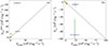 |
Fig. 9. Comparison of nonlinear energy transfer rate estimates obtained as the average LPDE |


5. Discussion and conclusions
This study demonstrates the critical role of anisotropy in space plasma energy transfer, showing that upcoming multipoint multiscale missions like HelioSwarm and Plasma Observatory are essential for accurate observations of the energy cascade rate in space.
We used hybrid PIC simulations to investigate Yaglom’s law and employed both single and multiple virtual spacecraft configurations. A benchmark solution, obtained via a finite-difference scheme across the entire simulation domain, served as reference.
Our simulations revealed that assuming isotropy, a common and necessary practice in single-spacecraft analyses, can lead to significant inaccuracies in estimating the nonlinear energy transfer rate using Yaglom’s law. The estimated energy transfer rate heavily depends on the angle between the spacecraft trajectory and the mean magnetic field. This finding highlights the inherent limitations of single-point measurements and corroborates previous numerical studies (Verdini et al. 2015).
Conversely, when multipoint multiscale measurements such as those planned for HS and PO are employed, we achieved a remarkably accurate retrieval of the scale-dependent behavior of the energy cascade rate. This was facilitated by the LPDE technique, which generates numerous thousands of estimates for the nonlinear energy transfer rate across various scales. While some solution spread exists, it is considerably smaller than that from a single spacecraft, thus enhancing the statistical reliability of the results obtained with this technique. As anticipated, the spread increased with the volume spanned by the spacecraft constellation, but the relative error remained consistent across all separations. Importantly, the averaged values at all scales closely matched the benchmark solution.
The analysis of Yaglom’s law in the parallel-perpendicular lag plane (relative to the mean magnetic field) demonstrated the expected elongation of the third-order structure function along the parallel direction. This indicates that nonlinear energy transfer is initiated at smaller scales in the perpendicular direction than in the parallel direction. This means that the energy cascade is more active toward smaller scales in the perpendicular direction while being inhibited in the parallel direction. The vast number of solutions from multiple spacecraft at different lags provides crucial insights into the anisotropy of Yaglom’s law, even within the limited scale range of the spacecraft configuration. Despite these limitations, which were recreated to be similar to those expected in space environments such as the solar wind and magnetosheath, these observatories will offer the first direct information on Yaglom’s law anisotropy in space plasma.
The anisotropy of Yaglom’s law is directly linked to the scale-dependent variation in the balance of terms within the vKH equation. The three terms in the vKH equation are proportional to the total energy cascade rate across all scales. Ideally, each term dominates a specific scale range: the time-dependent term at large scales, the nonlinear term in the inertial range, and the dissipative term at very small scales. Consequently, anisotropy in any term implies an anisotropic scale-dependent overlap between them. This agrees with other numerical work on the Yaglom flux anisotropy (Verdini et al. 2015) and inertial range extension (Wang et al. 2022; Jiang et al. 2023; Hellinger et al. 2024; Jiang et al. 2025).
We note that the directional variability of the plateau in Yaglom’s law relates directly to the efficacy of this method in the identification of the inertial range. The scaling of the third-order structure function is an exact result from Kolmogorov’s theory, in contrast to the second (and higher)-order structure function, which instead requires intermittency corrections (Frisch 1995). Thus, an accurate determination of the inertial range is attained by using the third-order moment, although its convergence requires larger statistics (Anselmet et al. 1984). The analogous analytical result was obtained for MHD (Politano & Pouquet 1998a) and the linear scaling observed in spacecraft observations (Bruno & Carbone 2005; Sorriso-Valvo et al. 2007; Marino et al. 2012).
We then applied the same methods to MMS data in the magnetosheath. Without a direct observational benchmark, our numerical results provide a framework for interpreting these findings. While MMS offers multipoint data, its configuration limits a multiscale analysis. We computed the PP law using single-spacecraft MMS observations and then applied LPDE to the four-spacecraft constellation to solve the 3D Yaglom law. An idealized behavior of the nonlinear term typically shows an increasing trend at the lower end of the inertial range, followed by a constant value. Our numerical simulations confirmed the reliability of LPDE in estimating the nonlinear energy transfer rate across all scales without additional assumptions, unlike the PP formulation, which is highly sensitive to the spacecraft orientation relative to the background magnetic field.
The MMS data revealed varying trends. The expected scale-dependent behavior of the transfer rate (patching together MMS sub-di estimates with larger-scale isotropic estimates) was only roughly recovered in intervals II, III, and IV. Moreover, isotropic estimates frequently showed alternating positive and negative values, with a notable prevalence of negative values. In contrast, LPDE consistently provided positive estimates for most intervals; only interval I showed a consistent negative LPDE energy transfer rate.
In an idealized scenario, a constant energy transfer rate value is expected within the inertial range. However, our comparison of average LPDE estimates with the isotropic maximum absolute and signed average values revealed inconsistencies: for three intervals, LPDE estimates at kinetic scales coincided with average inertial range values, which is unexpected, as the nonlinear energy transfer from Yaglom’s law should be larger in the inertial range. Moreover, using the isotropic signed average, one interval showed a higher LPDE value than anticipated. It has been suggested that positive and negative energy fluxes may coexist (Marino & Xie 2025) in the inertial range. This circumstance might help explain some of the current observations.
The examination of the angle between the plasma flow speed and the magnetic field provided some order. Intervals with the most inconsistent behavior (I and V) had the most aligned or anti-aligned flows. Conversely, intervals showing more consistent scale-dependent trends (II and III) had more perpendicular sampling directions. These results are consistent with our numerical investigations and warrant further statistical analysis.
In conclusion, our findings confirm the importance of accounting for anisotropy when estimating energy transfer in space plasmas. This work anticipates a paradigmatic shift in space plasma studies with the advent of future multipoint multiscale missions. The consistent results from virtual HS and PO configurations support the feasibility of these analyses in both the solar wind and magnetosphere, even with a reduced number of spacecraft in case of failures. The simultaneous presence of HS and PO will provide solar wind and magnetosphere investigations on an unprecedentedly similar footing. These missions will fundamentally revolutionize space plasma data analysis, enabling the extraction of previously unattainable information within the inner heliosphere.
Acknowledgments
This work was supported by NASA MMS Mission Theory, Modeling and Data Analysis Program under grant number 80NSSC19K0565 and NSF SHINE grant 2501387 at the University of Delaware, and the plan for NASA EPSCoR Research Infrastructure Development (RID) in Delaware (NASA award 80NSSC22M0039). This study was conducted using the numerical facility at the Delaware Space Observation Center (DSpOC), which is supported by NASA Awards 80NSSC22K0884 and 80NSSC23K0608. P.H. acknowledges grant 25-17802S of the Czech Science Foundation. This work was supported by the Ministry of Education, Youth and Sports of the Czech Republic through the e-INFRA CZ (ID:90254). K.G.K was partially supported by NASA contract 80ARC021C0001.
References
- Adhikari, S., Shay, M. A., Parashar, T. N., et al. 2023, Phys. Plasmas, 30, 082904 [Google Scholar]
- Adhikari, S., González, C. A., Yang, Y., et al. 2025, ApJ, 992, 180 [Google Scholar]
- Andrés, N., & Sahraoui, F. 2017, Phys. Rev. E, 96, 053205 [CrossRef] [Google Scholar]
- Andrés, N., Sahraoui, F., Galtier, S., et al. 2019, Phys. Rev. Lett., 123, 245101 [CrossRef] [Google Scholar]
- Andrés, N., Sahraoui, F., Huang, S., Hadid, L. Z., & Galtier, S. 2022, A&A, 661, A116 [NASA ADS] [CrossRef] [EDP Sciences] [Google Scholar]
- Angelopoulos, V. 2008, Space Sci. Rev., 141, 5 [Google Scholar]
- Angelopoulos, V. 2011, Space Sci. Rev., 165, 3 [Google Scholar]
- Anselmet, F., Gagne, Y., Hopfinger, E. J., & Antonia, R. A. 1984, J. Fluid Mech., 140, 63 [NASA ADS] [CrossRef] [Google Scholar]
- Balogh, A., Dunlop, M. W., Cowley, S. W. H., et al. 1997, Space Sci. Rev., 79, 65 [CrossRef] [Google Scholar]
- Bandyopadhyay, R., Chasapis, A., Chhiber, R., et al. 2018a, ApJ, 866, 81 [NASA ADS] [CrossRef] [Google Scholar]
- Bandyopadhyay, R., Chasapis, A., Chhiber, R., et al. 2018b, ApJ, 866, 106 [Google Scholar]
- Batchelor, G. K. 1953, The theory of homogeneous turbulence (Cambridge University Press) [Google Scholar]
- Bourouaine, S., & Perez, J. C. 2018, ApJ, 858, L20 [Google Scholar]
- Broeren, T., Klein, K. G., & TenBarge, J. M. 2024, Earth Space Sci., 11, e2023EA003369 [Google Scholar]
- Bruno, R., & Carbone, V. 2005, Liv. Rev. Sol. Phys., 2, 4 [Google Scholar]
- Burch, J. L., Moore, T. E., Torbert, R. B., & Giles, B. L. 2016, Space Sci. Rev., 199, 5 [CrossRef] [Google Scholar]
- Carbone, V., Marino, R., Sorriso-Valvo, L., Noullez, A., & Bruno, R. 2009, Phys. Rev. Lett., 103, 061102 [NASA ADS] [CrossRef] [Google Scholar]
- Chasapis, A., Matthaeus, W. H., Parashar, T. N., et al. 2017, ApJ, 844, L9 [NASA ADS] [CrossRef] [Google Scholar]
- Chhiber, R., Chasapis, A., Bandyopadhyay, R., et al. 2018, J. Geophys. Res. (Space Phys.), 123, 9941 [Google Scholar]
- Chhiber, R., Usmanov, A. V., Matthaeus, W. H., Parashar, T. N., & Goldstein, M. L. 2019, ApJS, 242, 12 [Google Scholar]
- Cuesta, M. E., Chhiber, R., Roy, S., et al. 2022, ApJ, 932, L11 [NASA ADS] [CrossRef] [Google Scholar]
- de Karman, T., & Howarth, L. 1938, Proc. Royal Soc. Lond. Ser. A Math. Phys. Sci., 164, 192 [Google Scholar]
- Dunlop, M., Southwood, D., Glassmeier, K.-H., & Neubauer, F. 1988, Adv. Space Res., 8, 273 [CrossRef] [Google Scholar]
- Dunlop, M. W., Fu, H.-S., Shen, C., et al. 2024, Front. Astron. Space Sci., 11, 2024 [Google Scholar]
- Ferrand, R., Galtier, S., Sahraoui, F., et al. 2019, ApJ, 881, 50 [NASA ADS] [CrossRef] [Google Scholar]
- Fox, N. J., Velli, M. C., Bale, S. D., et al. 2016, Space Sci. Rev., 204, 7 [Google Scholar]
- Franci, L., Verdini, A., Matteini, L., Landi, S., & Hellinger, P. 2015, ApJ, 804, L39 [Google Scholar]
- Franci, L., Hellinger, P., Guarrasi, M., et al. 2018a, J. Phys. Conf. Ser., 1031, 012002 [Google Scholar]
- Franci, L., Landi, S., Verdini, A., Matteini, L., & Hellinger, P. 2018b, ApJ, 853, 26 [Google Scholar]
- Fredricks, R. W., & Coroniti, F. V. 1976, J. Geophys. Res. (1896–1977), 81, 5591 [Google Scholar]
- Frisch, U. 1995, Turbulence: the legacy of AN Kolmogorov (Cambridge University Press) [Google Scholar]
- Galtier, S. 2008, Phys. Rev. E, 77, 015302 [CrossRef] [Google Scholar]
- Hadid, L. Z., Sahraoui, F., & Galtier, S. 2017, ApJ, 838, 9 [Google Scholar]
- Hadid, L. Z., Sahraoui, F., Galtier, S., & Huang, S. Y. 2018, Phys. Rev. Lett., 120, 055102 [NASA ADS] [CrossRef] [Google Scholar]
- Hellinger, P., Verdini, A., Landi, S., Franci, L., & Matteini, L. 2018, ApJ, 857, L19 [NASA ADS] [CrossRef] [Google Scholar]
- Hellinger, P., Papini, E., Verdini, A., et al. 2021, ApJ, 917, 101 [NASA ADS] [CrossRef] [Google Scholar]
- Hellinger, P., Verdini, A., Montagud-Camps, V., et al. 2024, A&A, 684, A120 [NASA ADS] [CrossRef] [EDP Sciences] [Google Scholar]
- Howes, G. G. 2008, Phys. Plasmas, 15, 055904 [Google Scholar]
- Isaacs, J. J., Tessein, J. A., & Matthaeus, W. H. 2015, J. Geophys. Res. Space Phys., 120, 868 [Google Scholar]
- Jiang, B., Li, C., Yang, Y., et al. 2023, J. Fluid Mech., 974, A20 [Google Scholar]
- Jiang, B., Gao, Z., Yang, Y., et al. 2025, arXiv e-print [arXiv:2512.16610] [Google Scholar]
- Jokipii, J. R. 1973, ARA&A, 11, 1 [Google Scholar]
- Klein, K. G., Perez, J. C., Verscharen, D., Mallet, A., & Chandran, B. D. G. 2015, ApJ, 801, L18 [Google Scholar]
- Klein, K. G., Spence, H., Alexandrova, O., et al. 2023, Space Sci. Rev., 219, 74 [Google Scholar]
- Klein, K. G., Broeren, T., Roberts, O., & Schulz, L. 2024, J. Geophys. Res. Space Phys., 129, e2024JA033428 [Google Scholar]
- Kolmogorov, A. N. 1941a, Proc. Math. Phys. Sci., 434, 15 [Google Scholar]
- Kolmogorov, A. N. 1941b, Proc. R. Soc. Lond., 434, 9 [Google Scholar]
- Lamriben, C., Cortet, P.-P., & Moisy, F. 2011, Phys. Rev. Lett., 107, 024503 [Google Scholar]
- MacBride, B. T., Forman, M. A., & Smith, C. W. 2005, ESA Spec. Publ., 592, 613 [Google Scholar]
- MacBride, B. T., Smith, C. W., & Forman, M. A. 2008, ApJ, 679, 1644 [NASA ADS] [CrossRef] [Google Scholar]
- Marcucci, M. F., & Retinò, A. 2024, EGU General Assembly Conf. Abstr., 11903 [Google Scholar]
- Marino, R., & Sorriso-Valvo, L. 2023, Phys. Rep., 1006, 1 [NASA ADS] [CrossRef] [Google Scholar]
- Marino, R., & Xie, J. H. 2025, Sci. Adv., 11, eadv8988 [Google Scholar]
- Marino, R., Sorriso-Valvo, L., Carbone, V., et al. 2008, ApJ, 677, L71 [NASA ADS] [CrossRef] [Google Scholar]
- Marino, R., Sorriso-Valvo, L., Carbone, V., et al. 2011, Planet. Space Sci., 59, 592 [NASA ADS] [CrossRef] [Google Scholar]
- Marino, R., Sorriso-Valvo, L., D’Amicis, R., et al. 2012, ApJ, 750, 41 [NASA ADS] [CrossRef] [Google Scholar]
- Matthaeus, W. H., & Velli, M. 2011, Space Sci. Rev., 160, 145 [Google Scholar]
- Matthaeus, W. H., Ghosh, S., Oughton, S., & Roberts, D. A. 1996, J. Geophys. Res. Space Phys., 101, 7619 [Google Scholar]
- Matthaeus, W. H., Dasso, S., Weygand, J. M., et al. 2005, Phys. Rev. Lett., 95, 231101 [NASA ADS] [CrossRef] [Google Scholar]
- Matthaeus, W. H., Dasso, S., Weygand, J. M., Kivelson, M. G., & Osman, K. T. 2010, ApJ, 721, L10 [Google Scholar]
- Matthaeus, W. H., Weygand, J. M., & Dasso, S. 2016, Phys. Rev. Lett., 116, 245101 [Google Scholar]
- Niehof, J. T., Plice, L., Levinson-Muth, P., & Ames Research Center 2024, https://doi.org/10.5281/zenodo.13887062 [Google Scholar]
- Osman, K. T., Wan, M., Matthaeus, W. H., Weygand, J. M., & Dasso, S. 2011, Phys. Rev. Lett., 107, 165001 [Google Scholar]
- Oughton, S., & Matthaeus, W. H. 2005, Nonlinear Proc. Geophys., 12, 299 [Google Scholar]
- Paschmann, G., & Daly, P. W. 1998, Analysis Methods for Multi-Spacecraft Data (ESA Publications Division for The International Space Science Institute) [Google Scholar]
- Pecora, F. 2024, Plasma Phys. Contr. Fus., 66, 125008 [Google Scholar]
- Pecora, F., Servidio, S., Primavera, L., et al. 2023a, ApJ, 945, L20 [NASA ADS] [CrossRef] [Google Scholar]
- Pecora, F., Yang, Y., Matthaeus, W. H., et al. 2023b, Phys. Rev. Lett., 131, 225201 [NASA ADS] [CrossRef] [Google Scholar]
- Pecora, F., Pucci, F., Malara, F., et al. 2024, ApJ, 970, L36 [Google Scholar]
- Pecora, F., Chhiber, R., Roy, S., et al. 2025a, JGR Space Phys, submitted [Google Scholar]
- Pecora, F., Matthaeus, W. H., Greco, A., et al. 2025b, Proc. Nat. Academy Sci., 122, e2519635122 [Google Scholar]
- Perez, J. C., Bourouaine, S., Chen, C. H. K., & Raouafi, N. E. 2021, A&A, 650, A22 [EDP Sciences] [Google Scholar]
- Pezzi, O., Liang, H., Juno, J. L., et al. 2021, MNRAS, 505, 4857 [NASA ADS] [CrossRef] [Google Scholar]
- Politano, H., & Pouquet, A. 1998a, Geophys. Res. Lett., 25, 273 [NASA ADS] [CrossRef] [Google Scholar]
- Politano, H., & Pouquet, A. 1998b, Phys. Rev. E, 57, R21 [CrossRef] [Google Scholar]
- Pollock, C., Moore, T., Jacques, A., et al. 2016, Space Sci. Rev., 199, 331 [CrossRef] [Google Scholar]
- Pope, S. B. 2000, Turbulent flows (Cambridge University Press) [Google Scholar]
- Quijia, P., Fraternale, F., Stawarz, J. E., et al. 2021, MNRAS, 503, 4815 [NASA ADS] [CrossRef] [Google Scholar]
- Retinò, A., Khotyaintsev, Y., Le Contel, O., et al. 2022, Exp. Astron., 54, 427 [CrossRef] [Google Scholar]
- Roberts, O. W., Alexandrova, O., Sorriso-Valvo, L., et al. 2022, J. Geophys. Res. Space Phys., 127, e2021JA029483 [Google Scholar]
- Ruiz, M. E., Dasso, S., Matthaeus, W. H., & Weygand, J. M. 2014, Sol. Phys., 289, 3917 [Google Scholar]
- Russell, C. T., Anderson, B. J., Baumjohann, W., et al. 2016, Space Sci. Rev., 199, 189 [NASA ADS] [CrossRef] [Google Scholar]
- Shebalin, J. V., Matthaeus, W. H., & Montgomery, D. 1983, J. Plasma Phys., 29, 525 [Google Scholar]
- Shen, C., Zeng, G., Kieokaew, R., & Zhou, Y. 2025, Ann. Geophys., 43, 115 [Google Scholar]
- Sorriso-Valvo, L., Marino, R., Carbone, V., et al. 2007, Phys. Rev. Lett., 99, 115001 [CrossRef] [Google Scholar]
- Stawarz, J. E., Smith, C. W., Vasquez, B. J., Forman, M. A., & MacBride, B. T. 2009, ApJ, 697, 1119 [NASA ADS] [CrossRef] [Google Scholar]
- Stawarz, J. E., Eastwood, J. P., Phan, T. D., et al. 2022, Phys. Plasmas, 29, 012302 [Google Scholar]
- Taylor, G. I. 1938, Proc. Roy. Soc. Lond. Ser. A Math. Phys. Sci., 164, 476 [Google Scholar]
- Tennekes, H., & Lumley, J. L. 1972, A first course in turbulence (MIT press) [Google Scholar]
- Usmanov, A. V., Matthaeus, W. H., Goldstein, M. L., & Chhiber, R. 2018, ApJ, 865, 25 [Google Scholar]
- Verdini, A., Grappin, R., Hellinger, P., Landi, S., & Müller, W. C. 2015, ApJ, 804, 119 [NASA ADS] [CrossRef] [Google Scholar]
- Verscharen, D., Klein, K. G., & Maruca, B. A. 2019, Liv. Rev. Sol. Phys., 16, 5 [Google Scholar]
- Wang, Y., Chhiber, R., Adhikari, S., et al. 2022, ApJ, 937, 76 [NASA ADS] [CrossRef] [Google Scholar]
- Yang, Y., Matthaeus, W. H., Roy, S., et al. 2022, ApJ, 929, 142 [NASA ADS] [CrossRef] [Google Scholar]
- Yang, Y., Matthaeus, W. H., Oughton, S., et al. 2024, MNRAS, 528, 6119 [Google Scholar]
A definition for the Reynolds number is the ratio of the nonlinear to the dissipative terms in the Navier-Stokes equations (Pope 2000). This number can be directly related to the extension of the turbulent inertial range (Yang et al. 2024).
Note that within the region in which Eq. (2) is valid, both sides are independent of the direction and magnitude of the lag vector ℓ. This is so even if the Yaglom flux Y± is anisotropic, e.g., in the presence of a mean magnetic field. However, in general, as is the case for the results shown here, the region of validity of Eq. (2) may be anisotropic.
All Tables
All Figures
|
Fig. 1. Orbital plot showing the precession of the HS (left) and PO (right) observatory trajectories around the Earth (⨁ for HS and blue dot for PO), with regions of interest highlighted in blue (magnetosphere), red (solar wind), and green (foreshock) for HS. The thick lines in the HS plot indicate hours with ideal 3D multiscale coverage. The specific configuration we analyzed is marked with a black (red) dot for HS (PO). At this scale, it is not possible to distinguish individual spacecraft trajectories. |
| In the text | |
|
Fig. 2. HS and PO relative position of the spacecraft within each observatory. For HS, the central hub is displayed in red, and positions are measured relative to it. For PO, positions are measured relative to the barycenter. |
| In the text | |
|
Fig. 3. HS and PO baseline magnitudes. For HS, kinetic, transition, and MHD ranges are indicated with color bands. For PO, only the kinetic range below 50 km is indicated with a shaded area. |
| In the text | |
|
Fig. 4. Scale-dependent energy cascade rate from Yaglom’s law using different methods. Grid-computed exact solution (red plus). We show single-s/c PP estimates at varying angles to B0 (green lines). We also show LPDE multi-s/c solutions (cyan cross) and the LPDE average (large blue cross), and the error bars indicate the standard deviation. Top: LPDE on smaller-scale HS. Bottom: LPDE on larger-scale HS. |
| In the text | |
|
Fig. 5. Relative standard deviation of LPDE measurements (bin average energy transfer rate |
| In the text | |
|
Fig. 6. (Top) Yaglom flux vector projected in the parallel-perpendicular increment plane. The arrows illustrate the transport of energy from large to small scales, consistent with a turbulent cascade that is predominantly active in the perpendicular direction. The arrow lengths are normalized by ℓ⊥ for visualization purposes, and the color reflects the non-normalized magnitude. (Bottom) Divergence of the Yaglom flux vector in the parallel-perpendicular increment plane. The elongated feature along the parallel direction is indicative of turbulent energy transfer more active in the perpendicular direction. |
| In the text | |
|
Fig. 7. Anisotropic energy cascade rate ϵ(ℓ⊥, ℓ∥) in the parallel-perpendicular increment plane (assuming gyrotropy). Top: Full simulation grid solution (benchmark). Middle: HS with smaller separations (kinetic scales). Bottom: HS with larger separations (inertial scales). Even with limited coverage, HS recovers the scale-dependent anisotropic trend. Different configurations cover different portions of the increment space. The coverage on the simulation grid and HS are delimited with solid and dashed gray boxes, respectively. The black lines are isocontours of the energy transfer rate. |
| In the text | |
|
Fig. 8. Estimates of Eq. (2) (filled blue circles for positive ϵ, and white circles for negative ϵ) using LPDE. The horizontal line is the average value (solid for positive, dashed for negative). The isotropic estimate from Eq. (3) (solid green lines for positive values, and dashed lines for negative values). The ion inertial length di and the correlation length λc are indicated in each panel. The different estimates of the isotropic cascade rate were obtained within the shaded green areas between 1.2di and 0.8λc. Panels (a)-(e) correspond to intervals I-V, respectively. |
| In the text | |
|
Fig. 9. Comparison of nonlinear energy transfer rate estimates obtained as the average LPDE |
| In the text | |
Current usage metrics show cumulative count of Article Views (full-text article views including HTML views, PDF and ePub downloads, according to the available data) and Abstracts Views on Vision4Press platform.
Data correspond to usage on the plateform after 2015. The current usage metrics is available 48-96 hours after online publication and is updated daily on week days.
Initial download of the metrics may take a while.