| Issue |
A&A
Volume 708, April 2026
|
|
|---|---|---|
| Article Number | A226 | |
| Number of page(s) | 17 | |
| Section | Galactic structure, stellar clusters and populations | |
| DOI | https://doi.org/10.1051/0004-6361/202557672 | |
| Published online | 08 April 2026 | |
Delayed phase mixing in the self-gravitating Galactic disc
1
Departament de Física Quàntica i Astrofísica (FQA), Universitat de Barcelona (UB),
c. Martí i Franquès, 1,
08028
Barcelona,
Spain
2
Institut de Ciències del Cosmos (ICCUB), Universitat de Barcelona (UB),
c. Martí i Franquès, 1,
08028
Barcelona,
Spain
3
Institut d’Estudis Espacials de Catalunya (IEEC),
c. Gran Capità 2–4,
08034
Barcelona,
Spain
★ Corresponding author: This email address is being protected from spambots. You need JavaScript enabled to view it.
Received:
13
October
2025
Accepted:
13
February
2026
Abstract
Context. The discovery of the phase spiral in the vertical position–velocity (z–vz) distribution of the solar neighbourhood stars revealed the Milky Way (MW) disc disequilibrium. The phase spiral is considered to work as a dynamical clock for dating past perturbations, but some previous studies neglected the disc self-gravity, which might bias estimates of the phase spiral excitation time.
Aims. We revisit self-gravitating effects on the evolution of vertical phase spirals and quantify the bias introduced in estimating their excitation time when these effects are ignored.
Methods. We analysed a high-resolution self-consistent N-body simulation of the MW interaction with the Sagittarius dwarf galaxy (Sgr), alongside four test-particle simulations in potentials constructed from the N-body snapshots. In the test-particle simulations, we used static and time-dependent potentials that included (or excluded) Sgr and the dark matter (DM) wake. In each case, we estimated the winding time of phase spirals by measuring the slope of the density contrast in the vertical angle–frequency (θz–Ωz) space.
Results. In test-particle models, the phase spiral immediately begins to wind after the Sgr pericentric passage, and the winding time closely tracks the true elapsed time since the Sgr pericentric passage. Adding the DM wake yields only a modest (<100 Myr) reduction of the winding time relative to Sgr alone. By contrast, the self-consistent N-body simulation exhibits an initial coherent vertical oscillation lasting ≳300 Myr before a clear spiral forms, leading to a systematic underestimation of the excitation times. An analytical shearing-box model with self-gravity, developed in a previous study, qualitatively reproduces this delay. This supports the hypothesis that it originates in the response of the self-gravitating disc.
Conclusions. Assuming that self-gravity affects phase mixing in the MW to the same degree as the N-body model, we estimated the lag induced by self-gravity to be ∼0.3 Gyr in the solar neighbourhood. Accounting for this delay revises the inferred age of the observed phase spiral of the MW to ∼0.6–1.2 Gyr, which agrees better with the Sgr pericentric passage. An accurate dynamical dating of past perturbations thus requires models that include the self-gravitating response of the Galactic disc.
Key words: methods: numerical / galaxy: disk / galaxy: kinematics and dynamics
© The Authors 2026
 Open Access article, published by EDP Sciences, under the terms of the Creative Commons Attribution License (https://creativecommons.org/licenses/by/4.0), which permits unrestricted use, distribution, and reproduction in any medium, provided the original work is properly cited.
This article is published in open access under the Subscribe to Open model. This email address is being protected from spambots. You need JavaScript enabled to view it. to support open access publication.
1 Introduction
The phase spiral is a spiral structure that is observed in the vertical position (z) versus vertical velocity (vz) space (Antoja et al. 2018). It is one of the most significant discoveries of the Gaia mission (Gaia Collaboration 2016). It provides direct evidence of the incomplete vertical phase mixing in the Milky Way (MW) disc and indicates that the MW disc is in a disequilibrium state due to strong perturbation events in the past. Although the properties of the phase spiral have been studied both theoretically and observationally since its initial discovery in Gaia Data Release 2 (DR2; Gaia Collaboration 2018), its origin remains under debate (see Hunt & Vasiliev 2025 for a review).
Of the various proposed scenarios, those involving external perturbations such as satellite galaxies, dark matter (DM) wakes, and DM sub-haloes have been studied most extensively. Of all potential external perturbers, the Sagittarius dwarf galaxy (Sgr; Ibata et al. 1994) is a strong candidate for the origin of the phase spiral, as it is the most massive satellite after the Magellanic Clouds and has a small pericentre distance of ∼20 kpc, but may have had several past pericentres (e.g. Law & Majewski 2010; Purcell et al. 2011; Dierickx & Loeb 2017; Vasiliev et al. 2021). The formation of phase spirals through Sgr-like interactions has been demonstrated by analytical calculations (Binney & Schönrich 2018; Bennett & Bovy 2021; Banik et al. 2022, 2023), test-particle simulations (e.g. Li 2021; Gandhi et al. 2022), N-body simulations (Laporte et al. 2019; Bland-Hawthorn et al. 2019; Bland-Hawthorn & Tepper-García 2021; Hunt et al. 2021; Bennett et al. 2022; Asano et al. 2025), and N-body+hydrodynamical simulations (Tepper-García et al. 2025). Additionally, phase spirals have been detected in cosmological simulations (García-Conde et al. 2022; Grand et al. 2023), although the masses and orbits of the satellites in these simulations do not necessarily correspond to those of Sgr due to the nature of cosmological modelling. As alternative explanations, small stochastic perturbations (Tremaine et al. 2023; Gilman et al. 2025; Tepper-García et al. 2025), bar buckling (Khoperskov et al. 2019), DM wake (Grand et al. 2023), and Galactic echoes1 (Chiba et al. 2025a) have also been proposed. Additionally, García-Conde et al. (2024) demonstrated that the dark sub-haloes, disc-halo misalignment, and anisotropic gas accretion can trigger disc bending and phase spirals by analysing cosmological simulations.
To investigate the origin of the phase spiral, it is crucial to accurately estimate the excitation time of the bending mode associated with the one-arm phase spiral. For example, when the estimated time coincides with the timing of the pericentric passage of Sgr within the uncertainties, this supports the Sgr scenario. When the times do not agree, the results might indicate that the phase spiral was instead excited by other perturbations. Assuming that the perturbation is impulsive and the gravitational potential remains static, we can estimate the formation time of the phase spiral by unwinding it, or in other words, by reconstructing its evolution backwards in time. Equivalently, this can be achieved by measuring the slopes of ridges in the vertical angle (θz) versus vertical frequency (Ωz) space, which correspond to the phase spirals in the z–vz space (Li & Widrow 2021; Darragh-Ford et al. 2023; Frankel et al. 2023; Lin et al. 2025). With these methods, the formation of the one-arm phase spiral has been estimated to have started ∼300–900 Myr ago (Antoja et al. 2023; Darragh-Ford et al. 2023; Frankel et al. 2023, 2025; Widmark et al. 2025).
However, these estimates can be significantly biased when the disc self-gravity is neglected. Darling & Widrow (2019) qualitatively compared the time evolution of phase spirals in a self-consistent N-body simulation with that in a test-particle simulation using a static potential similar to that of the N-body model. They found that the phase spiral in the N-body model is less tightly wound than in the test-particle model. Widrow (2023) analytically investigated the effect of self-gravity on two-arm and one-arm phase spirals. In the case of a breathing perturbation, which is associated with the two-arm phase spiral, the evolution is complex; not only does the initially excited phase spiral wind up, but new phase spirals are generated by swing amplification of the surface density perturbation. Furthermore, the study showed that static (non-winding) two-arm phase spirals can exist around massive clouds. In contrast, for a bending perturbation, which is associated with the one-arm phase spiral, the model does not predict such a complicated evolution. Instead, it shows that the phase spiral winds up more slowly than in kinematic (non-self-gravitating) models, as observed in the simulations by Darling & Widrow (2019).
In Asano et al. (2025), we performed high-resolution N-body simulations of the MW-Sgr system and visually examined the time evolution and spatial variation of phase spirals. We found that two-arm phase spirals appear intermittently, while one-arm phase spirals wind up in a more orderly manner (see Fig. 12 of Asano et al. 2025). The relatively regular evolution of the one-arm phase spiral compared to the two-arm phase spiral in the analytical model (Widrow 2023) and N-body simulations suggests that it can be used as a dynamical clock to date past perturbations in the MW disc. However, to use it reliably, the effects of self-gravity must be accounted for. As a first step in this direction, this paper aims to quantitatively evaluate the bias introduced when self-gravitating effects are ignored. In addition, we provide an empirical correction of the unwinding method in order to incorporate self-gravity. We analyse the N-body simulation (Asano et al. 2025), which employs 200 million particles in the disc (and 4.9 billion particles in the DM halo). This high-resolution N-body model allows us to track the long-term (∼1 Gyr) self-gravitating evolution of phase spirals.
The structure of this paper is as follows. Section 2 describes the N-body and test-particle simulations and qualitatively discusses the evolution of the phase spirals in both types of simulation. Section 3 presents our unwinding method and applies it to the simulations. We show the winding time as a function of time and phase-space position (guiding radius and azimuthal angle), and compare it between the N-body and test-particle models. Section 4 compares the results with an analytical shearing-box model including self-gravity, discusses the origin of the delayed winding, and considers the implications for the MW. Section 5 provides our conclusions.
2 Simulations
2.1 N-body simulation
We used the N-body model of the MW-Sgr interaction from Asano et al. (2025)2. The MW-like host galaxy consists of a classical bulge, a stellar disc, and a DM halo, which follow a Hernquist profile (Hernquist 1990), a radially exponential and vertically sech2 profile, and a Navarro–Frenk–White (NFW) profile (Navarro et al. 1997), respectively. The initial condition was generated using the Galactics code (Kuijken & Dubinski 1995; Widrow & Dubinski 2005; Widrow et al. 2008). The model parameters are identical to those of Fujii et al. (2019)’s best-fit MW model, MWa. The masses of the components are Mbulge = 5.4 × 10⁹M⊙, Mdisc = 3.6 × 10¹⁰M⊙, and Mhalo = 8.7 × 10¹¹M⊙. Each component consists of equal-mass particles of ~170M⊙, with a total number of particles of 5.1 billion. The initial condition of the Sgr-like satellite was modelled as a combination of a stellar component with a Hernquist profile and a DM component with an NFW profile. Their initial masses were Mstar = 1 × 10⁹M⊙ and MDM = 5 × 10¹⁰ M⊙, respectively.
In Asano et al. (2025), we first integrated the MW model in isolation for 8 Gyr to reach a quasi-steady state, then injected the satellite at r ∼ 150 kpc and simulated their interaction for ∼3 Gyr. The satellite experienced three pericentric passages with pericentre distances of ∼20, 13, and 10 kpc. Its position about 30 Myr after the second pericentric passage was close to the present-day location of Sgr (see Fig. 2 of Asano et al. 2025). The orbit is nearly polar, with an orbital plane roughly aligned with the x–z plane, and the satellite crosses the disc shortly before the first pericentric passage. This disc crossing occurs at (R, ϕ) ∼ (25 kpc, 0°). We primarily focused on the time interval between the first and second pericentric passages. We performed the simulation on Pegasus at the Center for Computational Sciences, University of Tsukuba, using the Bonsai code (Bédorf et al. 2012, 2014). Further details of the simulation can be found in Asano et al. (2025).
The fundamental properties of the simulated Galactic disc, such as the rotation curve and the velocity dispersion, are consistent with those of the MW. Therefore, we expect the effect of self-gravity on the evolution of the phase spiral to be similar to that in the real Galaxy, although additional contributions from the gaseous components can further modify the evolution (Tepper-García et al. 2022, 2025).
We computed actions, angles, and orbital frequencies of the MW stellar particles using Agama (Vasiliev 2019) with the Stäckel fudge method (Binney 2012). To do this, we constructed an axisymmetric potential model from the N-body snapshot at 300 Myr before the first pericentric passage of Sgr, using a potential expansion that is described in the next subsection.
2.2 Test-particle simulations
We constructed potential models from the previous N-body snapshots with Agama to run test-particle simulations. For the disc and the bulge, we constructed static axisymmetric potentials from the N-body snapshot taken 300 Myr before the first pericentric passage of Sgr. At this time, Sgr is sufficiently distant from the Galactic centre, and its effect on the disc is negligible. We applied an azimuthal harmonic expansion to the disc and a multipole expansion to the bulge. For the DM halo of MW, we constructed both static and time-dependent potentials. The static potential was derived from the same snapshot as we used for the stellar component through an axisymmetric multipole expansion. The time-dependent potential was obtained by interpolating the non-axisymmetric potentials from individual N-body snapshots, whose output cadence of ∼10 Myr is sufficiently short to resolve the time evolution of the potential. For Sgr, we first performed multipole expansions in the Sgr-centric frame and then transformed the potential into the MW-centric frame. We also applied temporal interpolation to the Sgr potential. For further details of the potential models, see Appendix A.
We performed four test-particle simulations using different combinations of these potential models. Table 1 summarises the model setup. We used snapshots of the N-body model as the initial conditions of the test-particle simulations. In the model with a purely static potential TP (static), we took the N-body snapshot at t = 0 Gyr, which is the time of the first Sgr pericentric passage. In the other models including the perturber potential, we took the snapshot at t = −300 Myr. In the TP (static) model, particles were perturbed only once at t = 0. They were then evolved in the fully static axisymmetric potential, without any further external perturbations. As a result, the subsequent evolution of the phase spiral in this model reflects purely kinematic phase mixing in a rigid potential. By contrast, in the other test-particle models, particles experienced continuous perturbations arising from the time-dependent gravitational effect of Sgr, the DM wake, or both, but self-gravity was absent in all of them.
Before presenting the results of the test-particle simulations, we first examine the characteristics of Sgr and the MW halo DM wake by evaluating the force field they generate. Since our interest lies in the internal motion of disc stars rather than their overall motion in an inertial frame, the perturbing force is given by
 (1)
(1)
where Φpert is the potential of the perturbers (i.e. Sgr and the DM wake). The first term corresponds to the force in an inertial frame, and the second term represents the acceleration of the coordinate system comoving with the MW disc. Figure 1 shows the vertical component of the perturbing force as a function of time. The force was evaluated along circular orbits at R = 8 kpc, and the colours of the curves indicate the azimuth ϕ = Ω8 kpct + ϕ0. The upper panel shows the contribution of Sgr. The curves show strong peaks around the times of the Sgr pericentric passages (t = 0 and t = 0.8 Gyr). At the first pericentric passage, the stars at ϕ ∼ 0° and ∼180° are kicked up and down (positive and negative vertical forces), respectively. The lower panel shows the contribution of the DM wake. The peak of the DM wake is shifted to a later time than the Sgr pericentric passage by ∼0.1 Gyr. Compared to the direct perturbation of Sgr, the wake induces a slightly weaker force at pericentre, but a more continuous force is present all the time.
We note that this behaviour contrasts with the results of the cosmological simulation by Grand et al. (2023), who found that the gravitational torque induced by the DM wake exceeds that from the satellite itself. This difference likely reflects variations in the adopted model setups. The strength of the DM wake is expected to depend on the satellite mass and orbit, as well as on the structure of the host halo, and the relative importance of the satellite and wake can also vary with time. For example, in the N-body simulation of the MW-Sgr system by Laporte et al. (2018), the DM wake dominates the torque during the first pericentric passage, whereas the direct contribution from Sgr becomes comparable to or stronger than that of the wake in subsequent passages (see Grion Filho et al. 2021 for an analysis of the force fields in that simulation). In the simulations by Grand et al. (2023) and Laporte et al. (2018) and also in ours, the peaks of the DM wake perturbation occur close to or with only a slight delay (≲100 Myr) relative to the peaks of the satellite perturbation. Regardless of which component dominates the instantaneous perturbation amplitude, the onset of vertical phase mixing is therefore expected to occur close to the pericentric passage time. As discussed below, the subsequent evolution of the phase spiral is more strongly affected by the disc self-gravity.
While Fig. 1 illustrates both the amplitude and direction (i.e. positive or negative) of the vertical perturbation along a ring at R = 8 kpc, Fig. 2 focuses on the amplitudes alone and presents it as a function of radius and time. We evaluated the amplitude by averaging the square of the vertical force,  , over azimuth. The first panel of Fig. 2 shows the amplitude of the Sgr perturbation. As we saw in Fig. 1, Sgr perturbs the disc during short time intervals around the pericentric passages. The influence of Sgr begins earlier and continues longer in the outer galaxy than in the inner galaxy. The map exhibits a narrow gap at t = −0.05 Gyr, when Sgr crosses the disc, and therefore, Fz,Sgr becomes zero. The second panel of the figure shows the same map for the DM wake. The amplitude of the wake starts to increase at t ∼ 0, reaches maximum at t ∼ 0.1 Gyr, and then decreases slowly. After reaching a minimum at t ∼ 0.4 Gyr, it starts to increase again and becomes almost constant from t ∼ 0.5 Gyr. In general, the DM halo response to a satellite galaxy can be decomposed into the dynamical friction wake and the collective response (see Appendix A and Garavito-Camargo et al. 2021). The dynamical friction wake is a transient over-density located behind the satellite along its orbit, while the collective response manifests as a large-scale dipole asymmetry in the DM halo that persists for a longer duration. In our model, the peak at t ∼ 0.1 Gyr and the subsequent long-lived component are attributed to the dynamical friction wake and the collective response, respectively. The third panel shows the ratio of the Sgr force to the wake force. The impact of the Sgr main body is confined in short time intervals around the pericentric passages, while the wake perturbation dominates during most of the time between the pericentric passages. Grion Filho et al. (2021) also analysed the force fields of the Sgr and the DM wake in the N-body model simulated by Laporte et al. (2018). Consistent with our model, the force profile of Sgr exhibits high-amplitude spikes around pericentric passages, whereas the DM force evolves more gradually.
Summary of the test-particle models.
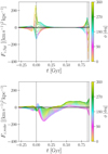 |
Fig. 1 Vertical forces due to Sgr (upper panel) and the DM wake (lower panel). The forces were evaluated along circular orbits at R = 8 kpc, and the colours of the lines indicate the azimuth ϕ = Ω8 kpct + ϕ0. The vertical dashed lines indicate the times of the Sgr pericentric passages. |
 |
Fig. 2 Amplitude of the perturbing force as a function of R and t. The colour maps represent the force amplitudes due to Sgr (first panel), the DM wake (second panel), and their ratio (third panel). The vertical dashed lines indicate the times of the Sgr pericentric passages. |
2.3 Phase spirals
We first visually inspect the phase spirals in both the N-body and test-particle simulations, although we quantify the differences between the models in the next section. Figure 3 presents the particle distributions in the  plane in an annulus at Rg = 8 ± 1 kpc, with the data binned by azimuthal angle. The
  map is a projection of vertical action–angle space, which is morphologically analogous to the z–vz phase-space map3. For the present sample, the extent of the distribution is comparable to the z–vz map with |z| ≲ 1 kpc and |vz| ≲ 50 km s−1. From top to bottom, the rows correspond to the TP (static), TP (Sgr), TP (wake), TP (Sgr+wake), and N-body models, respectively. The snapshots are taken at t ∼ 0.4 Gyr, which corresponds to the epoch at which the phase-spiral patterns can be identified most clearly across all models. Each panel shows the density contrast relative to the symmetric background density. We estimated the background density by randomising θz of the particles within each azimuthal angle (θϕ) bin.
All models exhibit one-arm phase spirals, although their prominence and tightness differ across the models. In the TP (static) and TP (Sgr) models, the phase spirals are wound tightly in a similar manner, whereas in the test-particle simulations with the DM wake, TP (wake) and TP (Sgr+wake), they appear less tightly wound. This is because the peak of the wake perturbation force is delayed relative to the Sgr pericentric passage, which introduces a delay in the phase mixing start (see Fig. 1).
Compared to the test-particle models, the phase-space maps of the N-body model are notably more complex. In many panels of the N-body model, the phase-space distribution resembles a superposition of a phase spiral and a dipole pattern. Although weak dipole-like asymmetries are also observed in the TP (wake) and TP (Sgr+wake) models (e.g. panels around θϕ ~ −120° to −40°), they are less pronounced than in the N-body case. We attribute this difference to the self-gravitating nature of the disc in the N-body simulation. As suggested by previous studies (Darling & Widrow 2019; Widrow 2023), the phase spiral in the N-body model is less tightly wound than in the test-particle models.
We also examine the temporal evolution of the phase spirals in Fig. 4. The columns represent different models, while the rows correspond to the different times between the first and second pericentric passages. In the TP (static) model, an initial dipole perturbation is progressively stretched via phase mixing and evolves into a tightly wound phase spiral. The TP (Sgr) model displays a similar evolution, but at t = 0.88 Gyr, a new dipole perturbation is triggered by Sgr’s second pericentric passage. In the TP (wake) model, there is no clear asymmetry in the distribution at t = 0 Gyr because the force of the wake has not yet reached its maximum and is not strong enough to excite the significant bending in the disc. A phase spiral forms at t = 0.10 Gyr and becomes increasingly tightly wound until t = 0.49 Gyr. Unlike the TP (Sgr) model, a new dipole pattern emerges at t = 0.59 Gyr. As shown in Appendix A, the DM wake consists of two distinct components: a transient dynamical friction wake and a collective response. These components imprint dipole-like signatures in the vertical phase space at different times. The first dipole pattern, which emerges at t ∼ 0.1 Gyr and evolves into the spiral, is triggered by the dynamical friction wake. The second dipole pattern appearing at t ≳ 0.5 Gyr is associated with the collective halo response. Since its perturbation is weaker and more slowly varying than that of the dynamical friction wake, it does not fully erase the pre-existing phase spiral, resulting in a superposition of the two features.
In the TP (Sgr+wake) model, the phase spiral initially resembles that of the TP (Sgr) model: a dipole pattern appears at t = 0 and develops into a one-arm spiral. At later times (0.5 ≲ t ≲ 0.8 Gyr), a new dipole pattern becomes visible that resembles the feature seen in the TP (wake) model, suggesting that the wake-driven perturbation dominates during this epoch.
In the N-body model, phase spirals do not form until t = 0.29 Gyr, a behaviour previously reported by Asano et al. (2025)4. In self-gravitating discs, dipole patterns excited by external perturbations tend to rotate almost rigidly before transforming into phase spirals. Subsequently, the phase spiral develops and winds up with time. In comparison to the test-particle models, the phase spirals in the N-body model are less tightly wound and more disordered. In particular, the centre of the spiral does not necessarily coincide with the origin of the adopted phase-space coordinate, and both the strength and width of the spiral show significant variations along it, in contrast to the more regular behaviour seen in the test-particle models. In the next section we quantitatively examine this non-monotonous phase mixing in self-gravitating systems.
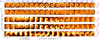 |
Fig. 3 Phase spirals in the TP (static) model (first row), TP (Sgr) model (second row), TP (wake) model (third row), TP (Sgr+wake) model (fourth row), and N-body model (fifth row). Each panel shows the density contrast in the |

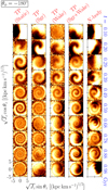 |
Fig. 4 Time evolution of the phase spiral. From top to bottom, the rows correspond to the different models TP (static), TP (Sgr), TP (wake), TP (Sgr+wake), and N-body model. From left to right, time increases from t = 0 Gyr to 0.88 Gyr. |
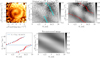 |
Fig. 5 Phase spiral unwinding. Top left: density contrast in the |


3 Unwinding phase spirals
3.1 Method
If stars oscillate vertically at frequencies constant with time, which depend only on their (primarily vertical) actions, a phase spiral observed in the z–vz space transforms into a stripe pattern in the θz–Ωz space, where θz and Ωz represent the vertical angle and vertical frequency, respectively. If a perturbation occurs at t = 0, the stripe pattern at a later time follows a simple linear relation: θz = Ωzt + θ0. By fitting this linear model to the data, we can estimate the winding time of the phase spiral, which corresponds to the time elapsed since the perturbation occurred. This unwinding method was adopted in several previous studies (e.g. Darragh-Ford et al. 2023; Frankel et al. 2023). In our work, we applied a similar approach to both our N-body and test-particle simulations. However, to ensure a robust fit, we first preprocessed the data, as described below. Here, we present the procedure using a noisy example from the N-body model to demonstrate the effectiveness of this processing, and also provide an idealised example from TP (static) model in Appendix B.
The top left panel of Fig. 5 shows an example of the particle distribution in  space from the N-body simulation at t = 0.39 Gyr. A one-arm phase spiral pattern can be identified in the distribution. In the middle top panel, we map the same distribution into the
  space. We divided this space into 30 × 90 bins, where the upper and lower boundaries of
  correspond to the 5th and 95th percentiles of the
  distribution, respectively. The colour of each pixel indicates the number density
  normalised by the mean density
  at each
  . The diagonal ridge pattern that appears in this projection corresponds to the phase spiral. In addition to the ridge, we see a vertical band between θz ~ π and ∼3/2π, which corresponds to the dipole asymmetry that extends across the entire region of the top left panel. While it is also an interesting feature and might reflect the self-gravitating nature of the disc or the DM wake perturbation, we leave it aside here.
To enhance the ridge pattern for robust fitting, in the following steps, we cleaned the  map. We subtracted the Gaussian-blurred map and applied the bilateral filter (Tomasi & Manduchi 1998) and contrast-limited adaptive histogram equalization (CLAHE; Pizer et al. 1987), using the opencv-python package. The filtered map is shown in the top right panel, with the pixel values scaled from 0 to 1. This image processing reduces both small-scale noise and large-scale bias, such as the global dipole asymmetry, and enhances the ridge pattern.
We next applied a Fourier transform to the filtered map along the θz axis,
![Mathematical equation: $\tilde n\left( {{J_z},{\theta _z}} \right) = \sum\limits_{k = - \infty }^\infty {{A_k}} \left( {{J_z}} \right)\exp \left[ { - ik\left( {{\theta _z} - {\theta _{z,k}}\left( {{J_z}} \right)} \right)} \right],$](/articles/aa/full_html/2026/04/aa57672-25/aa57672-25-eq18.png) (2)
(2)
where ñ is the pixel value in the filtered image, and Ak and θz,k are the amplitude and the phase of the k-th Fourier mode, respectively. The red dots in the top right panel indicate the phase of the k = 1 mode, θz,1, which traces the ridges (i.e. one-arm phase spiral)5. We also show the results of Fourier transform for the unfiltered map in the top middle panel with cyan dots. Without filtering, the k = 1 phase does not trace the ridge, demonstrating the effectiveness of our filtering procedure.
We mapped the detected k = 1 phase into the θz–Ωz space shown in the bottom left panel. The horizontal and vertical coordinates of the dots show the θz,1 and mean Ωz values in each  bin, respectively. We fitted these data with the function
 (3)
(3)
by minimising the error function
 (4)
(4)
where N = 30 is the number of the  bins, and j is the index of the bins. We found the best-fit (tfit, θ0) using scipy.optimize.differential_evolution. The blue line in the bottom left panel shows the fitting result, and the bottom right panel shows the
  map reconstructed from the fitting result. The winding time, tfit, which corresponds to the slope of the ridges in θz–Ωz space, is equal to the time elapsed since a perturbation is applied if phase mixing proceeds without influence of self-gravity.
As illustrated in Figs. 3 and 4, phase spirals are not always well defined. To exclude such cases from the analysis, we evaluated the quality of the Fourier-based pattern recognition and the fitting using two metrics. The first one is the fitting error defined by Eq. (4). The second one is the Structural Similarity Index Measure (SSIM; Wang et al. 2004), which quantifies structural similarity between two images in a manner consistent with human visual perception. We measured the SSIM between the reconstructed map (bottom right panel) and the filtered map (top right panel). We excluded fitting results from the analysis when the fitting error E(tfit, θ0) > 0.2 and the SSIM < 0.4. These thresholds were selected based on the cases where the ridge detection failed clearly according to visual comparison of the  maps, the fitting results, and the corresponding metric values.
3.2 Results
We first examine the TP (Sgr+wake) model. We divided the Rg–θϕ space into bins of 0.5 kpc × 10° and computed the winding time, tfit, in each bin. Figure 6 shows tfit across six snapshots, covering the time span from t = 0 to 0.9 Gyr. Equivalent plots from the other test-particle models are shown in Appendix C. At t = 0 (top left panel), tfit is consistent with zero in most bins, except within a narrow range around θϕ ~ 230°, which is stronger at outer radii. This region corresponds∼ to the location in which the effect of Sgr first becomes apparent (see Fig. 1). As time progresses, the winding time increases almost monotonically from t = 0 to 0.49 Gyr. However, diagonal narrow bands emerge, roughly following the curve −Ω(Rg)t + 230° (indicated by red curves). This pattern reflects the shearing of the initial azimuthal variations due to the differential disc rotation. The TP (static) model, shown in Fig. C.1, exhibits a much more uniform distribution of tfit within each R–θϕ plane. This confirms that the azimuthal variations seen in the TP (Sgr+wake) model arise from time-dependent, azimuthally varying perturbations. At t = 0.68 Gyr, regions with tfit ∼ 0 Gyr appear around θϕ ∼ 180°. We see that this originates from the DM wake perturbation because an equivalent feature is seen in the TP (wake) model but absent in the TP (Sgr) model (see Fig. C.2). In the last panel (t = 0.88 Gyr), tfit drops to zero across most bins because the impact of the second pericentric passage dominates over that of the first one. This behaviour indicates that each pericentric passage effectively resets the dynamical clock if the mass of the perturber remains sufficiently large. Similar behaviour has been reported in previous studies (Laporte et al. 2019; Bland-Hawthorn et al. 2019; García-Conde et al. 2022).
Figure 7 presents analogous maps for the N-body model. As shown in Fig. 4, in this case, phase spirals remain absent for some time following the first pericentric passage of Sgr. Consistent with this, tfit remains near zero not only at t = 0 Gyr but also at t = 0.10 Gyr. A rise in tfit begins at t = 0.29 Gyr, though this increase is not as monotonic as in the TP (Sgr+wake) case: now it progresses more rapidly in the inner disc than in the outer regions. At t = 0.49 Gyr, tfit remains systematically lower in the outer disc compared to the inner disc. By t = 0.68 Gyr, tfit has reached ∼0.4 Gyr across most of the disc between Rg ~ 7 kpc and 12 kpc. At t = 0.88 Gyr, tfit again drops to zero, reflecting the second pericentric passage of Sgr.
In general, we find that the winding time of the phase spiral in the TP (Sgr+wake) model (Fig. 6) increases almost monotonically with time, with values consistent with the elapsed time since the Sgr pericentric passage. In contrast, in the N-body model (Fig. 7), the winding time evolves non-linearly and stays below the actual time elapsed since the pericentric passage.
We next compare the winding time of the phase spiral in the N-body and test-particle models more quantitatively. We extract the columns at Rg = 8–8.5 kpc from the same maps shown in Figs. 6, 7, C.1, and C.2, and derive the distributions of tfit across the azimuthal angles, θϕ. Figure 8 shows these distributions for the TP (static), TP (Sgr), TP (Sgr+wake), and N-body models. Here, we do not include the TP (wake) model in the figure because adding it would cause overlap with other histograms and reduce readability. Each row corresponds to a different time, indicated in the bottom right corner of each panel and marked with black vertical lines. To obtain smooth histograms, we applied a Gaussian kernel density estimate (KDE) using scipy.stats.gaussian_kde (Virtanen et al. 2020).
In the TP (static) model (pink), the distribution peaks of tfit coincide with t (vertical lines) up to t = 0.49 Gyr, as expected from a pure one-dimensional phase mixing model. At later times, the peaks shift towards shorter times, but the difference is less than ∼50 Myr. A possible explanation for this small discrepancy is the effect of phase mixing in the radial and azimuthal directions. The satellite perturbation introduces not only vertical but also in-plane disturbances to disc stars, which are associated with tidally induced spiral arms (Antoja et al. 2022; Bernet et al. 2025) and radial phase spirals (Hunt et al. 2024). The coupling between vertical and in-plane motions might cause the small deviation of tfit from t.
In the TP (Sgr) model (yellow), the behaviour is similar to that of the TP (static) model, with peaks of tfit remaining close to t. At t = 0.78 Gyr and t = 0.88 Gyr, the distributions return to tfit ∼ 0 in response to the second pericentric passage of Sgr.
The overall trend in the TP (Sgr+wake) model (green) resembles that of the TP (Sgr) model. However, the peak values of tfit are systematically lower between t = 0.29 Gyr and 0.68 Gyr. In this epoch, the DM wake perturbation dominates over that of Sgr. The distribution in the TP (Sgr+wake) model is also broader than in the TP (Sgr) model.
In contrast, the N-body model (purple) exhibits a significantly different evolution. From t = 0 to 0.29 Gyr, the distribution remains concentrated at tfit ∼ 0, with little change in dispersion. Thereafter, the distribution begins to broaden and shift towards higher tfit values. The peak values of tfit in this case are substantially lower than in the test-particle models, and the distributions show higher dispersion, indicating greater azimuthal variation. In the N-body model, tfit falls to zero at t = 0.88 Gyr in response to the second pericentric passage, whereas in the TP (Sgr+wake) model it has already returned to zero by t = 0.78 Gyr. This offset implies a delayed response of the self-gravitating disc to external perturbations, as the external forces in the two models are essentially identical within the accuracy of the potential expansion.
We finally examine the radial and temporal evolution of the winding time of the phase spiral. We computed the azimuthal average of tfit over θϕ in each bin of Rg and t, and show the relative value, ⟨tfit⟩ − t, with respect to the true elapsed time in Fig. 9.
In the TP (static) model (top left panel), ⟨tfit⟩ − t is nearly zero, although it becomes slightly negative in the inner disc at t ≳ 0.8 Gyr. As discussed above, this small (<50 Myr) deviation is likely due to horizontal mixing. In the TP (Sgr) model (top middle panel), similar to the TP (static) case, ⟨tfit⟩ − t stays close to zero until t = 0.7 Gyr, after which it drops rapidly to negative values in response to the second pericentric passage of Sgr. In the TP (wake) model (top right panel), ⟨tfit⟩ − t is negative across all bins, with differences of ∼150–200 Myr for t ≲ 0.6 Gyr. Unlike the TP (Sgr) model, the TP (wake) model does not show a radially coherent, sharp drop at the time of the second pericentric passage. The TP (Sgr+wake) model (bottom left panel) exhibits combined behaviour from both the TP (Sgr) and TP (wake) cases. Up to t ∼ 0.6 Gyr, ⟨tfit⟩ − t is slightly negative, with differences less than 100 Myr. From t ~ 0.7 Gyr, the response to the DM wake becomes evident, starting from the outer disc. By the final snapshot, ⟨tfit⟩ drops to zero, and thus ⟨tfit⟩ − t becomes very negative, reflecting the second pericentric passage of Sgr. Finally, ⟨tfit⟩ − t in the N-body model (bottom right panel) is also negative across all bins as in the TP (wake) and TP (Sgr+wake) models. However, while the offset in the previous cases remains below 100 Myr, in the N-body model it reaches ~200–400 Myr, for instance at t = 0.5 Gyr.
To conclude, in the test-particle models, the winding time is slightly shorter than the elapsed time since the Sgr pericen-tric passage because the peak of the DM wake perturbation lags behind the pericentric passage of the Sgr main body. The underestimation in the N-body model (∼200–400 Myr) is even larger than in the TP (Sgr+wake) model (≲100 Myr), suggesting that the less wound phase spirals seen in the N-body simulation cannot be explained by the DM wake alone, but are likely the result of self-gravitating effects of the disc. Darragh-Ford et al. (2023) also found the same order of offset between the winding time and the peak time of the Sgr perturbation in the N-body model by Hunt et al. (2021). Their results also suggest that self-gravity contributes to the less wound phase spirals.
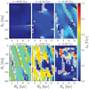 |
Fig. 6 Winding time of the phase spiral as a function of guiding radius, Rg, and azimuthal angle, θϕ, in the TP (Sgr+wake) model. The six panels correspond to different snapshots from t = 0 to 0.88 Gyr. In each panel, bins with poorly defined phase spirals (i.e. E > 0.2 and SSIM < 0.4) are masked with hatching. The red curves in the panels at t = 0, 0.10, 0.29, and 0.49 Gyr indicate θϕ = Ω(Rg)t + 230°. |
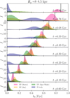 |
Fig. 8 Distribution of the winding time tfit in the ring Rg = 8– 8.5 kpc. The filled pink, yellow, green, and purple areas represent KDE-smoothed distributions for the TP (static), TP (Sgr), TP (Sgr+wake), and N-body models, respectively. Each row corresponds to a different time, separated by ∼0.1 Gyr. The vertical lines indicate the actual time elapsed since the first pericentric passage. |
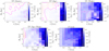 |
Fig. 9 Mean winding time of the phase spiral as a function of Rg and t in the TP (static) (top left), TP (Sgr) (top middle), TP (wake) (top right), TP (Sgr+wake) (bottom left), and N-body (bottom right) models. The colours and contours indicate the mean winding time, ⟨tfit⟩, relative to the elapsed time since the first pericentric passage of Sgr. |
4 Discussion
4.1 Analytical models
We observed that phase spirals in the N-body model wind up more slowly than those in test-particle models, due to the self-gravitating effects of the disc. Widrow (2023) predicted this behaviour by using an analytical model, which is an extension of the shearing sheet framework and swing amplification model (Julian & Toomre 1966; Toomre 1981; Binney 2020) to three dimensions. In this we compare the predictions of the analytical model with the results of our N-body simulation. We adopt model parameters corresponding to those at R = 8.25 kpc in the N-body model. Technical details of the model are provided in Appendix D.
Figure 10, which is similar to Figs. 8 and 9 of Widrow (2023), illustrates the time evolution of the phase spiral in the kinematic (i.e., without self-gravity) and self-gravitating models. The colour map represents the perturbed term of the distribution function, f1(Jz, θz), in the  space. As discussed in Widrow (2023), the amplitudes of f1 in the self-gravitating models are greater than those in the kinematic models. However, we here focus on differences in the winding rates rather than the amplitudes. Therefore, we normalised the colour scale by the maximum absolute value of f1 for each model at each time.
The external potential excites a dipole moment in the distribution function at t = 0, as shown in the top-left panel. In the kinematic model, this dipole winds up at a constant rate and evolves into a tightly wound phase spiral. In contrast, in the self-gravitating model, the spiral begins to wind later, at t ~ 0.15 Gyr. Prior to that, the dipole moment rotates nearly rigidly. When comparing the phase spirals in the two models at the same time step, the self-gravitating case appears to be less wound. This model successfully reproduces the qualitative evolution of phase spirals observed in the N-body simulation.
We compute the winding time of the phase spiral in the analytical model by measuring the slope of the stripes in θz–Ωz space, as described in Sect. 3.1. Figure 11 presents the winding time as a function of time. If self-gravity can be neglected, tfit is equal to t as indicated by the blue dotted lines. In the analytical self-gravitating model, tfit remains approximately zero until t ∼ 0.15 Gyr. Thereafter, it increases at a rate comparable to that of the kinematic model (i.e. dtfit/dt ∼ 1). The N-body model exhibits qualitatively similar behaviour; however, quantitatively, the winding time is shorter than in the self-gravitating analytical model. In the N-body simulation, tfit begins to increase around t ∼ 0.2–0.3 Gyr, which is later than in the analytical model. The offset between the winding time and the true elapsed time is ∼0.2 Gyr in the analytical model, whereas it is ~0.3 Gyr in the N-body model at later times. This difference mainly arises from the variation in the duration of the initial non-winding phase between the two models.
There are several possible reasons for this discrepancy. Firstly, the analytical model assumes a simple impulsive plane-wave perturbation, whereas the external perturbation in the N-body model is more complex. Secondly, we adopted a simplified potential in the analytical model. Specifically, a single lowered isothermal model is used to represent the unperturbed vertical potential and density. In contrast, the vertical potential in the N-body model arises from a combination of the stellar disc and DM halo. Consequently, the potential employed in the analytical model might not precisely correspond to that of the N-body model. Furthermore, the model assumes a separable potential in the analytical model, while in reality, the radial and vertical components of the potential are coupled. Thirdly, the shearing box framework is a linear model, but non-linear effects might affect the winding rate of the phase spirals in the N-body model.
Incorporating such effects is not straightforward and lies beyond the scope of this study. Most importantly, however, the analytical model – even with its simplified assumptions – qualitatively reproduces the delayed winding of the phase spirals observed in the N-body model.
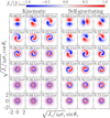 |
Fig. 10 Analytical phase spiral model. Time evolution of the |

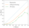 |
Fig. 11 Comparison of the winding times of the phase spirals in the analytical model and the N-body model. The dotted blue and solid orange lines represent the values from the kinematic and self-gravitating models, respectively. The green dots connected with dashed lines represent the azimuthally averaged winding time ⟨tfit⟩ at the bin of Rg = 8–8.5 kpc in the N-body model. The drop in tfit at t ∼ 0.8 Gyr in the N-body model is caused by the second pericentric passage, which is not taken into account in the analytical model. |
4.2 Implications for the Milky Way
We have shown that self-gravity effectively reduces the winding rates of phase spirals, and that the winding time estimated from purely kinematic models is significantly shorter than the actual time elapsed since the disc was perturbed. To use the observed phase spiral as a reliable dynamical clock, it is necessary to construct a time-evolution model that accounts for the self-gravity of the disc. The analytical model by Widrow (2023) and our N-body model suggest that there is a time lag between the excitation of the bending mode (caused by a close encounter with a dwarf galaxy) and the emergence of the phase spiral. During this initial stage of the bending mode evolution, the dipole phase-space pattern rotates almost rigidly (i.e. the disc oscillates coherently), and the phase spiral is not well-defined. Following this non-winding phase, the phase spirals begin to wind at a rate comparable to that predicted by the kinematic model. Based on this observation, we propose that the elapsed time can be approximated by
 (5)
(5)
where tfit is the winding time estimated from the slope in the θz– Ωz space, and ∆t is the time lag associated with the non-winding phase.
We naively expect that ∆t scales with a characteristic timescale associated with the stellar vertical oscillations. To test this expectation, we overplot a line representing the vertical epicycle period, 2π/ν, and its multiples on the ⟨tfit⟩ map of the N-body model in Fig. 12. In this figure, we show the absolute value of ⟨tfit⟩, in contrast to the relative value ⟨tfit⟩ − t shown in Fig. 9. At all radii, the winding time increases slowly until it reaches ⟨tfit⟩ ∼ 0.1 Gyr, which corresponds to the non-winding phase, and the time required for ⟨tfit⟩ to reach this value is equivalent to ∆t.
In our N-body model, ∆t is ~3–4 × 2π/ν. This factor likely depends on dynamical parameters related to self-gravity, such as Toomre’s Q and the vertical velocity dispersion. We cannot directly apply the analytical model to estimate this factor because we saw the discrepancies between the analytical and N-body models in the previous subsection. Qualitatively, the factor is expected to be smaller in hotter discs and larger in colder discs. Our N-body simulation is based on the best-fit MW model of Fujii et al. (2019), whose dynamical properties are consistent with recent observations of the MW. Therefore, we expect the time-lag factor in the real MW to be similarly close to 3–4. The vertical epicycle frequency in the solar neighbourhood is estimated to be ν ∼ 70 km s−1 kpc−1 (Binney & Tremaine 2008), which gives a time lag of ∆t ∼ 0.3 Gyr.
Previous studies have estimated the winding time of the phase spiral in the MW to be approximately 0.3–0.9 Gyr (Antoja et al. 2018, 2023; Darragh-Ford et al. 2023; Frankel et al. 2023). We therefore estimate the total elapsed time since the excitation of the bending mode to be telapsed ∼ 0.6–1.2 Gyr. Sgr is currently near pericentre, and its previous pericentric passage is estimated to have occurred ∼1–1.5 Gyr ago (Vasiliev et al. 2021). Thus, our estimate of the elapsed time (despite uncertainties in the lag) agrees more closely with the Sgr pericentric passage than previous estimates that did not account for self-gravity effects.
Recently, Widmark et al. (2025) measured the properties of the phase spiral, including the winding time, across the local disc within ≲4 kpc of the Sun using the Gaia DR3 dataset. They found that the observed winding time increases with Rg. This contrasts with our N-body simulation result, which showed that the azimuthally averaged winding time decreases with Rg (see Fig. 12). This discrepancy might arise from the observational selection function: the Gaia data only cover a limited azimuthal range (roughly ±25° around the Sun-Galaxy centre line). Figure 7 illustrates a substantial variation in the winding time with azimuthal angle in our N-body model, suggesting that the dependence on Rg may change when restricted to a limited azimuthal range rather than the entire disc. This indicates that both the azimuthal and radial dependence of the time lag ∆t in Eq. (5) must be taken into account in order to use the phase spiral as a reliable dynamical clock.
Finally, we note the possible effect of the gas disc, which is not included in our N-body model. The presence of gas alters the gravitational potential of the disc and can also modify the damping rate of disc oscillations through dissipative processes (Tepper-García et al. 2022). Due to these effects, the inclusion of a gas disc can change the time lag ∆t. Furthermore, N-body+gas simulations by Tepper-García et al. (2025) demonstrated that phase spirals can be generated by stochastic perturbations in turbulent gas disc via the mechanism proposed by Tremaine et al. (2023). These results suggest that phase spirals in the MW disc might not be attributable to the Sgr impact alone. We need further investigations with high-resolution N-body+gas simulations to understand the formation and evolution of phase spirals in more realistic discs.
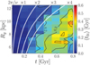 |
Fig. 12 Mean winding time of the phase spiral ⟨tfit⟩ as a function of guiding radius, Rg, and time, t, in the N-body model. The white curves represent t = (1, 2, 3, 4) × 2π/ν(Rg). |
5 Conclusions
We investigated the time evolution of vertical phase spirals in the Galactic disc using high-resolution N-body and test-particle simulations of the MW-Sgr interaction. Our goal was to quantify the bias introduced when self-gravitating effects are neglected in the dynamical modelling of vertical phase mixing in the Galactic disc:
In contrast to test-particle simulations, where phase spirals start to wind up promptly after perturbation, the self-consistent N-body model exhibits a delayed response. In the N-body model, the dipole pattern in the vertical phase-space distribution, excited by Sgr, initially rotates almost rigidly before transitioning into a winding phase spiral. This non-winding phase (coherent oscillation) causes a systematic underestimation of the excitation time;
The DM wake induces a more gradual and sustained perturbation than the Sgr impulsive effect. Although it affects the phase spiral morphology, it cannot fully account for the delayed and less tightly wound spirals observed in the N-body model. This suggests that self-gravity and not the DM wake primarily causes the slower phase mixing observed in the N-body disc;
The winding time (tfit) inferred from the slope in the vertical angle–frequency (θz–Ωz) space is consistently shorter than the true elapsed time since the Sgr pericentric passage. In the N-body model, tfit generally increases with the guiding radius, although there is a substantial variation across the azimuthal angle. The discrepancy between the winding time and the true elapsed time reaches ≳ 300 Myr at a guiding radius of Rg ~ 8 kpc;
The analytical self-gravitating model of Widrow (2023) reproduces the delayed winding of our model qualitatively, supporting the conclusion that self-gravity plays a central role in shaping the evolution of phase spirals;
In the N-body model, the amount of the self-gravity-induced delay is about three to four times the vertical epicycle period (2π/ν). When we assume that phase mixing is delayed on the same order in the MW, the time lag in the solar neighbourhood is estimated to be ∼0.3 Gyr. When this is combined with the winding time of the observed phase spiral (~0.3–0.9 Gyr), the inferred elapsed time since the excitation of the bending mode increases to ∼0.6–1.2 Gyr. Although substantial variations and uncertainties remain, this revised estimate agrees better with the timing of the previous pericentric passage of Sgr and supports the hypothesis that Sgr triggered the observed phase spiral.
We proposed a practical correction for the dynamical clock model of the phase spiral: telapsed ≈ tfit + ∆t, where tfit is the winding time inferred from kinematic analysis, and ∆t accounts for the non-winding phase caused by self-gravity. Future work should explore how this time lag depends on the dynamical properties of the Galactic disc and assess the applicability of this correction using N-body models under varying conditions. It is essential to incorporate self-gravity for robustly tracing the dynamical history of the MW.
Acknowledgements
We thank the anonymous referee for constructive comments that improved this manuscript. This project was developed in part at the “Winding, Unwinding and Rewinding the Gaia Phase Spiral” workshop hosted by the Lorentz Center in August 2025, Leiden, The Netherlands. This research used computational resources of Pegasus and Cygnus provided by Multidisciplinary Cooperative Research Program in Center for Computational Sciences, University of Tsukuba. We acknowledge the grants PID2021-125451NA-I00 and CNS2022-135232 funded by MICIU/AEI/10.13039/501100011033 and by “ERDF A way of making Europe”, by the “European Union” and by the “European Union Next Generation EU/PRTR”. This work made use of the following software packages: astropy (Astropy Collaboration 2013, 2018; Astropy Collaboration 2022), Jupyter (Perez & Granger 2007; Kluyver et al. 2016), matplotlib (Hunter 2007), numpy (Harris et al. 2020), pandas (Wes McKinney 2010; The pandas development team 2024), scipy (Virtanen et al. 2020; Gommers et al. 2023), Agama (Vasiliev 2019), and opencv-python (https://github.com/opencv/opencv-python). This research has made use of NASA’s Astrophysics Data System. Software citation information aggregated using The Software Citation Station (?Wagg et al. 2024).
References
- Antoja, T., Helmi, A., Romero-Gómez, M., et al. 2018, Nature, 561, 360 [Google Scholar]
- Antoja, T., Ramos, P., López-Guitart, F., et al. 2022, A&A, 668, A61 [NASA ADS] [CrossRef] [EDP Sciences] [Google Scholar]
- Antoja, T., Ramos, P., García-Conde, B., et al. 2023, A&A, 673, A115 [NASA ADS] [CrossRef] [EDP Sciences] [Google Scholar]
- Asano, T., Fujii, M. S., Baba, J., Portegies Zwart, S., & Bédorf, J. 2025, A&A, 700, A109 [NASA ADS] [CrossRef] [EDP Sciences] [Google Scholar]
- Astropy Collaboration (Robitaille, T. P., et al.) 2013, A&A, 558, A33 [NASA ADS] [CrossRef] [EDP Sciences] [Google Scholar]
- Astropy Collaboration (Price-Whelan, A. M., et al.) 2018, AJ, 156, 123 [Google Scholar]
- Astropy Collaboration (Price-Whelan, A. M., et al.) 2022, ApJ, 935, 167 [NASA ADS] [CrossRef] [Google Scholar]
- Banik, U., Weinberg, M. D., & van den Bosch, F. C. 2022, ApJ, 935, 135 [NASA ADS] [CrossRef] [Google Scholar]
- Banik, U., van den Bosch, F. C., & Weinberg, M. D. 2023, ApJ, 952, 65 [Google Scholar]
- Bédorf, J., Gaburov, E., Fujii, M. S., et al. 2014, in Proceedings of the International Conference for High Performance Computing, 54 [Google Scholar]
- Bédorf, J., Gaburov, E., & Portegies Zwart, S. 2012, J. Computat. Phys., 231, 2825 [Google Scholar]
- Bennett, M., & Bovy, J. 2021, MNRAS, 503, 376 [NASA ADS] [CrossRef] [Google Scholar]
- Bennett, M., Bovy, J., & Hunt, J. A. S. 2022, ApJ, 927, 131 [NASA ADS] [CrossRef] [Google Scholar]
- Bernet, M., Ramos, P., Antoja, T., et al. 2025, A&A, 702, A223 [NASA ADS] [CrossRef] [EDP Sciences] [Google Scholar]
- Binney, J. 2012, MNRAS, 426, 1324 [Google Scholar]
- Binney, J. 2020, MNRAS, 496, 767 [NASA ADS] [CrossRef] [Google Scholar]
- Binney, J., & Tremaine, S. 2008, Galactic Dynamics, 2nd edn. [Google Scholar]
- Binney, J., & Schönrich, R. 2018, MNRAS, 481, 1501 [Google Scholar]
- Bland-Hawthorn, J., & Tepper-García, T. 2021, MNRAS, 504, 3168 [CrossRef] [Google Scholar]
- Bland-Hawthorn, J., Sharma, S., Tepper-Garcia, T., et al. 2019, MNRAS, 486, 1167 [NASA ADS] [CrossRef] [Google Scholar]
- Chiba, R., Ding, J., Hamilton, C., Kunz, M. W., & Tremaine, S. 2025a, MNRAS, 543, 190 [Google Scholar]
- Chiba, R., Frankel, N., & Hamilton, C. 2025b, MNRAS, 543, 2159 [Google Scholar]
- Darling, K., & Widrow, L. M. 2019, MNRAS, 484, 1050 [CrossRef] [Google Scholar]
- Darragh-Ford, E., Hunt, J. A. S., Price-Whelan, A. M., & Johnston, K. V. 2023, ApJ, 955, 74 [NASA ADS] [CrossRef] [Google Scholar]
- Dierickx, M. I. P., & Loeb, A. 2017, ApJ, 836, 92 [NASA ADS] [CrossRef] [Google Scholar]
- Frankel, N., Bovy, J., Tremaine, S., & Hogg, D. W. 2023, MNRAS, 521, 5917 [NASA ADS] [CrossRef] [Google Scholar]
- Frankel, N., Hogg, D. W., Tremaine, S., Price-Whelan, A., & Shen, J. 2025, ApJ, 987, 81 [Google Scholar]
- Fujii, M. S., Bédorf, J., Baba, J., & Portegies Zwart, S. 2019, MNRAS, 482, 1983 [NASA ADS] [CrossRef] [Google Scholar]
- Gaia Collaboration (Prusti, T., et al.) 2016, A&A, 595, A1 [NASA ADS] [CrossRef] [EDP Sciences] [Google Scholar]
- Gaia Collaboration (Brown, A. G. A., et al.) 2018, A&A, 616, A1 [NASA ADS] [CrossRef] [EDP Sciences] [Google Scholar]
- Gandhi, S. S., Johnston, K. V., Hunt, J. A. S., et al. 2022, ApJ, 928, 80 [NASA ADS] [CrossRef] [Google Scholar]
- Garavito-Camargo, N., Besla, G., Laporte, C. F. P., et al. 2021, ApJ, 919, 109 [NASA ADS] [CrossRef] [Google Scholar]
- García-Conde, B., Roca-Fàbrega, S., Antoja, T., Ramos, P., & Valenzuela, O. 2022, MNRAS, 510, 154 [Google Scholar]
- García-Conde, B., Antoja, T., Roca-Fàbrega, S., et al. 2024, A&A, 683, A47 [NASA ADS] [CrossRef] [EDP Sciences] [Google Scholar]
- Gilman, D., Bovy, J., Frankel, N., & Benson, A. 2025, ApJ, 980, 24 [Google Scholar]
- Gommers, R., Virtanen, P., Haberland, M., et al. 2023, https://doi.org/10.5281/zenodo.10155614 [Google Scholar]
- Gould, R. W., O’Neil, T. M., & Malmberg, J. H. 1967, Phys. Rev. Lett., 19, 219 [Google Scholar]
- Grand, R. J. J., Pakmor, R., Fragkoudi, F., et al. 2023, MNRAS, 524, 801 [NASA ADS] [CrossRef] [Google Scholar]
- Grion Filho, D., Johnston, K. V., Poggio, E., et al. 2021, MNRAS, 507, 2825 [NASA ADS] [CrossRef] [Google Scholar]
- Harris, C. R., Millman, K. J., van der Walt, S. J., et al. 2020, Nature, 585, 357 [NASA ADS] [CrossRef] [Google Scholar]
- Hernquist, L. 1990, ApJ, 356, 359 [Google Scholar]
- Hunt, J. A. S., & Vasiliev, E. 2025, New A Rev., 100, 101721 [Google Scholar]
- Hunt, J. A. S., Stelea, I. A., Johnston, K. V., et al. 2021, MNRAS, 508, 1459 [NASA ADS] [CrossRef] [Google Scholar]
- Hunt, J. A. S., Price-Whelan, A. M., Johnston, K. V., et al. 2024, MNRAS, 527, 11393 [Google Scholar]
- Hunter, J. D. 2007, Comput. Sci. Eng., 9, 90 [NASA ADS] [CrossRef] [Google Scholar]
- Ibata, R. A., Gilmore, G., & Irwin, M. J. 1994, Nature, 370, 194 [Google Scholar]
- Julian, W. H., & Toomre, A. 1966, ApJ, 146, 810 [NASA ADS] [CrossRef] [Google Scholar]
- Khoperskov, S., Di Matteo, P., Gerhard, O., et al. 2019, A&A, 622, L6 [NASA ADS] [CrossRef] [EDP Sciences] [Google Scholar]
- Kluyver, T., Ragan-Kelley, B., Pérez, F., et al. 2016, in IOS Press, 87 [Google Scholar]
- Kuijken, K., & Dubinski, J. 1995, MNRAS, 277, 1341 [CrossRef] [Google Scholar]
- Laporte, C. F. P., Johnston, K. V., Gómez, F. A., Garavito-Camargo, N., & Besla, G. 2018, MNRAS, 481, 286 [Google Scholar]
- Laporte, C. F. P., Minchev, I., Johnston, K. V., & Gómez, F. A. 2019, MNRAS, 485, 3134 [Google Scholar]
- Law, D. R., & Majewski, S. R. 2010, ApJ, 714, 229 [Google Scholar]
- Li, Z.-Y. 2021, ApJ, 911, 107 [NASA ADS] [CrossRef] [Google Scholar]
- Li, H., & Widrow, L. M. 2021, MNRAS, 503, 1586 [CrossRef] [Google Scholar]
- Lin, J., Li, Z.-Y., Guo, R., et al. 2025, ApJ, 988, 254 [Google Scholar]
- Mulder, W. A. 1983, A&A, 117, 9 [NASA ADS] [Google Scholar]
- Navarro, J. F., Frenk, C. S., & White, S. D. M. 1997, ApJ, 490, 493 [Google Scholar]
- Perez, F., & Granger, B. E. 2007, Comput. Sci. Eng., 9, 21 [Google Scholar]
- Pizer, S. M., Amburn, E. P., Austin, J. D., et al. 1987, Comput. Vis., Graph. Image Process., 39, 355 [Google Scholar]
- Purcell, C. W., Bullock, J. S., Tollerud, E. J., Rocha, M., & Chakrabarti, S. 2011, Nature, 477, 301 [Google Scholar]
- Tepper-García, T., Bland-Hawthorn, J., & Freeman, K. 2022, MNRAS, 515, 5951 [CrossRef] [Google Scholar]
- Tepper-García, T., Bland-Hawthorn, J., Bedding, T. R., Federrath, C., & Agertz, O. 2025, MNRAS, 542, 1987 [Google Scholar]
- The pandas development team, 2024, https://zenodo.org/records/10537285 [Google Scholar]
- Tomasi, C., & Manduchi, R. 1998, in Sixth International Conference on Computer Vision (IEEE Cat. No. 98CH36271), IEEE, 839 [Google Scholar]
- Toomre, A. 1981, in Structure and Evolution of Normal Galaxies, eds. S. M. Fall, & D. Lynden-Bell, 111 [Google Scholar]
- Tremaine, S., Frankel, N., & Bovy, J. 2023, MNRAS, 521, 114 [NASA ADS] [CrossRef] [Google Scholar]
- Vasiliev, E. 2019, MNRAS, 482, 1525 [Google Scholar]
- Vasiliev, E. 2023, Galaxies, 11, 59 [NASA ADS] [CrossRef] [Google Scholar]
- Vasiliev, E., Belokurov, V., & Erkal, D. 2021, MNRAS, 501, 2279 [NASA ADS] [CrossRef] [Google Scholar]
- Virtanen, P., Gommers, R., Oliphant, T. E., et al. 2020, Nat. Med., 17, 261 [Google Scholar]
- Wagg, T., Broekgaarden, F., & Gültekin, K. 2024, [arXiv:2406.04405] [Google Scholar]
- Wang, Z., Bovik, A. C., Sheikh, H. R., & Simoncelli, E. P. 2004, IEEE Trans. Image Process., 13, 600 [Google Scholar]
- Weinberg, M. D. 1986, ApJ, 300, 93 [NASA ADS] [CrossRef] [Google Scholar]
- Weinberg, M. D. 1989, MNRAS, 239, 549 [NASA ADS] [CrossRef] [Google Scholar]
- Wes McKinney. 2010, in Proceedings of the 9th Python in Science Conference, eds. S. van der Walt, & J. Millman, 56 [Google Scholar]
- Widmark, A., Tavangar, K., Kalish, J., Johnston, K. V., & Hunt, J. A. S. 2025, arXiv e-prints [arXiv:2507.19579] [Google Scholar]
- Widrow, L. M. 2023, MNRAS, 522, 477 [NASA ADS] [CrossRef] [Google Scholar]
- Widrow, L. M., & Dubinski, J. 2005, ApJ, 631, 838 [Google Scholar]
- Widrow, L. M., Pym, B., & Dubinski, J. 2008, ApJ, 679, 1239 [Google Scholar]
A Galactic echo is an analogue of a plasma echo (Gould et al. 1967). These echoes are generated in collisionless systems that experience two successive perturbations due to the non-linear coupling between the first and second perturbations. For further details, see Chiba et al. (2025a).
The simulation data are available at http://galaxies.astron.s.u-tokyo.ac.jp/data/mwsgr.
For the harmonic oscillator, one has  and
and  . In general Galactic potentials, this correspondence is a good approximation only for orbits with small vertical amplitudes, but the resulting map exhibits a phase spiral morphology similar to that in the z-vz plane (see, for example, Fig. 1 of Darragh-Ford et al. 2023).
The delayed emergence of phase spirals is also observed in other self-consistent simulations (Bland-Hawthorn & Tepper-García 2021; Tepper-García et al. 2025).
We can measure θz–Ωz slope for the k = 2 mode (i.e. two-arm phase spirals) in the same way as for the k = 1 mode, but it does not necessarily correspond to the elapsed time since the excitation of the perturbation (see Widrow 2023 and Chiba et al. 2025b).
Appendix A Potential models
Here we provide details of the construction of the gravitational potential models. They were derived from N-body snapshots using the Agama library (Vasiliev 2019). Table A.1 summarises the Agama’s potential expansion parameters adopted for each component. For all parameters not listed, we used the default values.
For the static axisymmetric potentials (MW disc, MW bulge, and the DM halo without the wake), we applied the potential expansion to the snapshot at t = −300 Myr, which is sufficiently prior to the first pericentric passage of Sgr. In contrast, for the MW halo model including the DM wake, we used potential expansions from all snapshots. To account for temporal evolution, we employed the Evolving modifier, which linearly interpolates the potential between adjacent time stamps. The gravitational potential of Sgr was constructed in the same way, but with the coordinate system shifted to the Sgr-centric frame. The centre of Sgr was defined as the density peak of its stellar component. When performing test-particle simulations, the Sgr potential was transformed back into the MW-centric frame and evolved in time using the Shifted and Evolving modifiers.
Parameters of the potential expansion.
To verify that the potential model adequately captures halo substructures, we reconstructed the density field of the MW halo from the potential expansion and computed the density contrast,
 (A.1)
(A.1)
where ρ and ρ0 are the densities of the MW halo models with and without the DM wake, respectively. The integration over y from −20 kpc to 20 kpc was chosen because the orbital plane of Sgr is approximately aligned with the x–z plane. Figure A.1 shows the projected density contrast at t = 0 Gyr, together with the projected density distribution of Sgr, also reconstructed from the potential expansion. The overall morphology of the density contrast is consistent with the expected response of a DM halo to a massive satellite. Similar features have been reported in previous studies of the MW halo response to the Large Magellanic Cloud (LMC) (see Vasiliev 2023 and references therein). In particular, Garavito-Camargo et al. (2021) presented a comparable density map based on their N-body simulations of the MWLMC interaction. In the figure, two characteristic features can be clearly identified. The first is an overdense region trailing the orbit of Sgr, which corresponds to a transient wake induced by dynamical friction (Mulder 1983; Weinberg 19861). The second is a large-scale dipole density pattern, characterised by an overdensity in the upper left and an underdensity in the lower right of the panel. This dipole arises from the reflex motion of the MW halo and can persist longer than the transient wake, as it is sustained by resonant effects and self-gravity (Weinberg 1989).
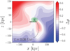 |
Fig. A.1 Milky Way halo density distribution reconstructed from the potential model. The background colour map indicates the density contrast defined by Eq. (A.1) at t = 0 Gyr. The green contours represent the projected density distribution of Sgr, showing in logarithmic scale between 10−2 and 100 of the maximum density. The horizontal black line and grey curve indicate the MW disc position and the orbital trajectory of Sgr, respectively. |
In Fig. A.2 we also present the same plot at t = 0.49 Gyr, when Sgr is close to its apocentre. We can identify the dynamical friction wake at (x, z) ∼ (−100, 50) kpc inside the collective response overdensity formed during the first infall. At this time, the centre of the dynamical friction wake is distant from the disc and its dynamical impact on the disc is considered to be relatively weaker than that of the collective response.
Appendix B Phase spiral fitting in the test particle model
We demonstrate that our phase spiral fitting method (Sect. 3.1) works accurately in ideal cases. We selected a particle sample from a bin with Rg = 7–7.5 kpc and θϕ = 150–160° in the snapshot at t = 0.39 Gyr from the TP (static) model, where the phase spiral is clearly visible. Figure B.1 illustrates the fitting procedure for this sample, following the same format as Fig. 5. In this case, the k = 1 Fourier mode of the original  distribution (top middle panel) already captures the diagonal ridge structure well, while the filtering further suppresses noise (top right panel). In the Ωz–θz space (bottom left panel), the extracted k = 1 mode forms straight lines. The winding time inferred from the fitting is tfit = 0.38 Gyr, in good agreement with the true elapsed time t = 0.39 Gyr.
Appendix C Supplementary figures from the test particle models
Figures C.1, C.2, and C.3 show the winding time of the phase spiral in the TP (static), TP (Sgr), TP (wake), and TP (Sgr+wake) models in the same manner as in Fig. 6.
Appendix D Shearing box model
The analytical framework developed by Widrow (2023) is based on linear perturbation theory within the shearing box approximation. This extends the classical shearing sheet formalism (Julian & Toomre 1966; Binney 2020) by incorporating vertical structure and self-gravity.
The shearing box is a local Cartesian coordinate system, x = (x, y, z), centred on a reference point at R = R0 and rotating with angular velocity Ω, where x denotes the radial direction, y the azimuthal direction, and z the vertical direction. The model assumes that the distribution function (DF) and gravitational potential can be decomposed into unperturbed and perturbed components:
 (D.1)
(D.1)
where f0 and Φ0 represent the time-independent unperturbed DF and potential, and f1 and Φ1 are linear perturbations. The perturbed potential Φ1 includes contributions from both external disturbances and the disc’s self-gravitating response.
Assuming epicyclic motion, the unperturbed Hamiltonian is expressed in separable form, H(x, p) = Hx + Hz, where p = (px, py, pz) is the momentum vector. The in-plane and vertical components of the Hamiltonian are defined as
 (D.2)
(D.2)
 (D.3)
(D.3)
where  is the guiding centre in the shearing box, κ is the epicyclic frequency, and Φz(z) is the vertical potential.
We adopt an unperturbed DF in which the in-plane and vertical components follow a Maxwell–Boltzmann and a lowered isothermal form, respectively:
 (D.4)
(D.4)
 (D.5)
(D.5)
where Σ0 is the surface density, σx and σz are the in-plane and vertical velocity dispersions, and  represents the thickness of the disc. The vertical density profile can be obtained by integrating Eq. (D.5) over pz, and the corresponding potential Φz(z) is obtained by solving Poisson’s equation.
The time evolution of the perturbed DF, f1, is governed by the linearised collisionless Boltzmann equation:
![Mathematical equation: ${{d{f_1}} \over {dt}} = {{\partial {f_1}} \over {\partial t}} + \left[ {{f_1},H} \right] = \left[ {{\Phi _1},{f_0}} \right],$](/articles/aa/full_html/2026/04/aa57672-25/aa57672-25-eq37.png) (D.6)
(D.6)
where the square brackets denote Poisson brackets. We integrate this equation along unperturbed orbits. By decomposing f1 into in-plane and vertical responses, Jp and Jz, we obtain
 (D.7)
(D.7)
 (D.8)
(D.8)
 (D.9)
(D.9)
where xp and pp are the in-plane position and momentum vectors, and ti is the time when the perturbation is initially applied. Assuming a plane-wave perturbation, the potential takes the form:
 (D.10)
where  is the vertical component of the potential and kp(t) = (kx, ky) is the in-plane wavevector. The phase kp · xp is constant along circular orbits, and if the shearing box is centred at the wave’s corotation radius, then
 (D.11)
where A is Oort’s first constant. We assume that the wavevector is aligned with the azimuthal direction at t = 0. The perturbed potential is related to the perturbed density  via a Green’s function solution of Poisson’s equation:
 (D.12)
and the vertical force is given by
 (D.13)
The vertical DF is defined by integrating  over pp:
 (D.14)
Using variable changes and Gaussian integrals (see Sect. 3 of Binney 2020), we obtained a Volterra integral equation,
 (D.15)
where the kernel Kp(t, t′) is given by
 (D.16)
with the Toomre parameter QT, and
![Mathematical equation: ${{\hat b}_x} = {{{k_y}} \over {{k_{{\rm{crit }}}}}}\left[ {A\left( {{t^\prime }\sin \kappa {t^\prime } - t\sin \kappa t} \right) + {\Omega \over \kappa }\left( {\cos \kappa {t^\prime } - \cos \kappa t} \right)} \right],$](/articles/aa/full_html/2026/04/aa57672-25/aa57672-25-eq51.png) (D.17)
(D.17)
![Mathematical equation: ${{\hat b}_y} = {{{k_y}} \over {{k_{{\rm{crit }}}}}}\left[ {A\left( {{t^\prime }\cos \kappa {t^\prime } - t\cos \kappa t} \right) - {\Omega \over \kappa }\left( {\sin \kappa {t^\prime } - \sin \kappa t} \right)} \right],$](/articles/aa/full_html/2026/04/aa57672-25/aa57672-25-eq52.png) (D.18)
(D.18)
where kcrit = κ2/(2πGΣ0). The vector c is defined as
 (D.19)
 (D.20)
The vertical response is given by
 (D.21)
where the vertical kernel is
 (D.22)
Up to this point, we have not assumed a specific vertical form for the external perturbation. If the perturbation kicks the north and south parts of the galactic disc in the same (opposite) direction, a bending (breathing) mode is excited. Since this study focuses on the one-arm phase spiral, in Sect. 4.1 we used the following antisymmetric external density perturbation following Sect. 3.2 of Widrow (2023):
 (D.23)
where Σe and ∆ correspond to the strength and vertical scale length of the perturbation, respectively. In the linear approximation, the winding rate of the phase spiral is independent of the perturbation strength Σe, which only affects the amplitude of the response. In the kinematic (non-self-gravitating) case, the perturbed density is  , while in the self-gravitating case,
  consists of
  and the self-gravitating term,
  .
.
We numerically solve the Volterra integral equations Eqs. (D.15) and (D.21). We adopt the parameters listed in Table D.1, which are chosen to match the local properties of our N-body model at Rg = 8.25 kpc.
Free parameters of the shearing box model.
All Tables
All Figures
|
Fig. 1 Vertical forces due to Sgr (upper panel) and the DM wake (lower panel). The forces were evaluated along circular orbits at R = 8 kpc, and the colours of the lines indicate the azimuth ϕ = Ω8 kpct + ϕ0. The vertical dashed lines indicate the times of the Sgr pericentric passages. |
| In the text | |
|
Fig. 2 Amplitude of the perturbing force as a function of R and t. The colour maps represent the force amplitudes due to Sgr (first panel), the DM wake (second panel), and their ratio (third panel). The vertical dashed lines indicate the times of the Sgr pericentric passages. |
| In the text | |
|
Fig. 3 Phase spirals in the TP (static) model (first row), TP (Sgr) model (second row), TP (wake) model (third row), TP (Sgr+wake) model (fourth row), and N-body model (fifth row). Each panel shows the density contrast in the |
| In the text | |
|
Fig. 4 Time evolution of the phase spiral. From top to bottom, the rows correspond to the different models TP (static), TP (Sgr), TP (wake), TP (Sgr+wake), and N-body model. From left to right, time increases from t = 0 Gyr to 0.88 Gyr. |
| In the text | |
|
Fig. 5 Phase spiral unwinding. Top left: density contrast in the |
| In the text | |
|
Fig. 6 Winding time of the phase spiral as a function of guiding radius, Rg, and azimuthal angle, θϕ, in the TP (Sgr+wake) model. The six panels correspond to different snapshots from t = 0 to 0.88 Gyr. In each panel, bins with poorly defined phase spirals (i.e. E > 0.2 and SSIM < 0.4) are masked with hatching. The red curves in the panels at t = 0, 0.10, 0.29, and 0.49 Gyr indicate θϕ = Ω(Rg)t + 230°. |
| In the text | |
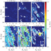 |
Fig. 7 Same as Fig. 6, but for the N-body model. |
| In the text | |
|
Fig. 8 Distribution of the winding time tfit in the ring Rg = 8– 8.5 kpc. The filled pink, yellow, green, and purple areas represent KDE-smoothed distributions for the TP (static), TP (Sgr), TP (Sgr+wake), and N-body models, respectively. Each row corresponds to a different time, separated by ∼0.1 Gyr. The vertical lines indicate the actual time elapsed since the first pericentric passage. |
| In the text | |
|
Fig. 9 Mean winding time of the phase spiral as a function of Rg and t in the TP (static) (top left), TP (Sgr) (top middle), TP (wake) (top right), TP (Sgr+wake) (bottom left), and N-body (bottom right) models. The colours and contours indicate the mean winding time, ⟨tfit⟩, relative to the elapsed time since the first pericentric passage of Sgr. |
| In the text | |
|
Fig. 10 Analytical phase spiral model. Time evolution of the |
| In the text | |
|
Fig. 11 Comparison of the winding times of the phase spirals in the analytical model and the N-body model. The dotted blue and solid orange lines represent the values from the kinematic and self-gravitating models, respectively. The green dots connected with dashed lines represent the azimuthally averaged winding time ⟨tfit⟩ at the bin of Rg = 8–8.5 kpc in the N-body model. The drop in tfit at t ∼ 0.8 Gyr in the N-body model is caused by the second pericentric passage, which is not taken into account in the analytical model. |
| In the text | |
|
Fig. 12 Mean winding time of the phase spiral ⟨tfit⟩ as a function of guiding radius, Rg, and time, t, in the N-body model. The white curves represent t = (1, 2, 3, 4) × 2π/ν(Rg). |
| In the text | |
|
Fig. A.1 Milky Way halo density distribution reconstructed from the potential model. The background colour map indicates the density contrast defined by Eq. (A.1) at t = 0 Gyr. The green contours represent the projected density distribution of Sgr, showing in logarithmic scale between 10−2 and 100 of the maximum density. The horizontal black line and grey curve indicate the MW disc position and the orbital trajectory of Sgr, respectively. |
| In the text | |
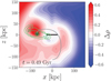 |
Fig. A.2 Same as Fig. A.1 but at t = 0.49 Gyr. |
| In the text | |
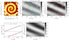 |
Fig. B.1 Phase spiral fitting example in the TP (static) model. Figure format is the same as Fig. 5. |
| In the text | |
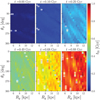 |
Fig. C.1 Same as Fig. 6 but for the TP (static) model. |
| In the text | |
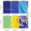 |
Fig. C.2 Same as Fig. 6 but for the TP (Sgr) model. |
| In the text | |
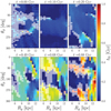 |
Fig. C.3 Same as Fig. 6 but for the TP (wake) model. |
| In the text | |
Current usage metrics show cumulative count of Article Views (full-text article views including HTML views, PDF and ePub downloads, according to the available data) and Abstracts Views on Vision4Press platform.
Data correspond to usage on the plateform after 2015. The current usage metrics is available 48-96 hours after online publication and is updated daily on week days.
Initial download of the metrics may take a while.