QSOFEED: Investigating warm molecular, low- and high-ionization atomic gas in six type-2 quasars with GTC/EMIR

P. H. Cezar; M. Coloma Puga; C. Ramos Almeida; J. A. Acosta-Pulido; G. Speranza; L. R. Holden; C. N. Tadhunter; M. V. Zanchettin; A. Audibert

doi:10.1051/0004-6361/202557799

Open Access

Issue		A&A Volume 708, April 2026


Article Number		A12
Number of page(s)		21
Section		Extragalactic astronomy
DOI		https://doi.org/10.1051/0004-6361/202557799
Published online		01 April 2026

A&A, 708, A12 (2026)

QSOFEED: Investigating warm molecular, low- and high-ionization atomic gas in six type-2 quasars with GTC/EMIR

P. H. Cezar¹^,2^★, M. Coloma Puga³^,4^,5, C. Ramos Almeida¹^,2, J. A. Acosta-Pulido¹^,2, G. Speranza⁶, L. R. Holden⁷, C. N. Tadhunter⁸, M. V. Zanchettin⁹ and A. Audibert¹^,2

¹ Instituto de Astrofísica de Canarias, Calle Vía Láctea, s/n, 38205 La Laguna, Tenerife, Spain
² Departamento de Astrofísica, Universidad de La Laguna, 38206 La Laguna, Tenerife, Spain
³ Dipartimento di Fisica, Università degli Studi di Torino, Via Pietro Giuria 1, 10125 (Torino), Italy
⁴ INAF – Osservatorio Astrofisico di Torino, Via Osservatorio 20, I-10025 Pino Torinese, Italy
⁵ European Southern Observatory (ESO), Alonso de Córdova 3107, Casilla 19, Santiago 19001, Chile
⁶ Instituto de Física Fundamental, CSIC, Calle Serrano 123, 28006 Madrid, Spain
⁷ Centre for Astrophysics Research, University of Hertfordshire, Hatfield AL10 9AB, United Kingdom
⁸ School of Mathematical and Physical Science, University of Sheffield, Sheffield S3 7RH, UK
⁹ INAF – Osservatorio Astrofisico di Arcetri, Largo E. Fermi 5, I-50125 Firenze, Italy

^★ Corresponding author: This email address is being protected from spambots. You need JavaScript enabled to view it.

Received: 22 October 2025
Accepted: 29 January 2026

Abstract

We present long-slit near-infrared spectroscopic observations of six nearby (z ∼ 0.1) radio-quiet type-2 quasars (QSO2s) from the Quasar Feedback (QSOFEED) sample. The QSO2s have bolometric luminosities of 10^{45 − 46} erg s⁻¹ and stellar masses of 10^10.6−11.3 M_⊙. The observations were obtained with the instrument Espectrógrafo Multiobjeto Infra-Rojo (EMIR) at the 10.4 m Gran Telescopio Canarias. The nuclear K-band spectra (central ∼1–3 kpc of the QSO2s) reveal signatures of high-velocity outflows in either the Paα or Brγ lines, depending on the redshift, and in the [Si VI] lines. The broadest kinematic components have a full width at half maximum (FWHM) of ∼1200–2500 km s⁻¹. From the near-infrared hydrogen recombination lines, we derived ionized outflow masses of M_Hion ∼ 0.08−20 × 10⁶ M_⊙, mass outflow rates of Ṁ_Hion ∼ 0.03−6 M_⊙ yr⁻¹, and kinetic powers of Ė_Hion ∼ 10^37.8−40.8 erg s⁻¹. These ionized gas outflow masses and mass outflow rates have median values that are 5.9 and 5.8 times larger, respectively, than those derived from the [Si VI] line. Our study provides evidence, at least for these six QSO2s, that the near-infrared recombination lines and [Si VI] trace the same outflow (i.e., they have similar kinematics and radii), but they carry different amounts of mass. We detected warm molecular lines in the six QSO2s, from which we measured total (nuclear) gas masses from 1.1 (0.7) to 32 (13) × 10³ M_⊙, similar to other QSO2s with warm H₂ measurements reported in the literature, but we did not find any molecular outflow associated with them. Based on comparison with five other QSO2s with H₂ measurements reported in the literature, we find that the four QSO2s with detected H₂ outflows have total (nuclear) H₂ masses that are 2.2 (2.7) times larger, on average, than the seven QSO2s without detected H₂ outflows.

Key words: galaxies: active / galaxies: evolution / galaxies: nuclei / quasars: emission lines

© The Authors 2026

Open Access article, published by EDP Sciences, under the terms of the Creative Commons Attribution License (https://creativecommons.org/licenses/by/4.0), which permits unrestricted use, distribution, and reproduction in any medium, provided the original work is properly cited.

This article is published in open access under the Subscribe to Open model. This email address is being protected from spambots. You need JavaScript enabled to view it. to support open access publication.

1. Introduction

Accreting supermassive black holes (SMBHs) in the nuclei of galaxies can undergo several accretion events (Hickox et al. 2014; Schawinski et al. 2015) during the life-cycle of galaxies, producing luminous activity episodes known as active galactic nuclei (AGN). The energy released in these recurrent AGN events can have significant effects on the host galaxy, the so-called AGN feedback. This feedback is capable of disturbing the gas kinematics (e.g., driving gas outflows) and producing changes in gas excitation and metallicity, thus ultimately impacting the formation of stars (see Harrison & Ramos Almeida 2024 for a recent review). Although AGN-driven outflows might lead to star formation quenching when they are powerful enough (negative feedback), simulations (Mercedes-Feliz et al. 2023) and observational works have also found evidence of positive feedback (i.e., AGN inducing star formation; Cresci et al. 2015a,b; Santoro et al. 2016; Maiolino et al. 2017; Gallagher et al. 2019; Bessiere & Ramos Almeida 2022). AGN feedback has become a key component for analytical and semi-analytical models and simulations (Harrison et al. 2018) to reproduce the observed Universe (Di Matteo et al. 2005; Davé et al. 2019; Su et al. 2019; Zinger et al. 2020; Zubovas & Maskeliūnas 2023).

To infer the impact of AGN feedback on galaxies, it is essential to determine how energy couples with the multiphase gas. Several studies, mostly focusing on optical emission lines, have reported the presence of ionized outflows (Villar-Martín et al. 2016; Fiore et al. 2017; Kakkad et al. 2020; Hervella Seoane et al. 2023; Speranza et al. 2024; Bertola et al. 2025), which appear to be ubiquitous, at least for luminous quasars (Harrison et al. 2014; Woo et al. 2016; Rupke et al. 2017; Bessiere et al. 2024). However, the role of outflows in other gas phases, which may be more relevant in terms of mass and energy budget, is still largely unconstrained in comparison with the ionized gas phase (Cicone et al. 2018). Besides, there is no consensus yet on whether or not the outflows detected in different phases are different faces of the same phenomenon (Harrison & Ramos Almeida 2024).

Coronal emission lines are important tracers of outflows in the highly ionized phase (see Rodríguez-Ardila & Cerqueira-Campos 2025 for a recent review). They are transitions of highly ionized species with an ionization potential (IP) ≳ 100 eV and mainly associated with AGN activity (but see Hernandez et al. 2025). Their usually high critical densities make them good outflow tracers closer to their launching region. Furthermore, Trindade Falcão et al. (2022) showed that coronal lines with IP > 138 eV could be used to trace the X-ray emitting-gas, confirming that these ions can probe the highest-ionized component of outflows. Despite their relevance, coronal line outflow studies are mostly restricted to nearby low-luminosity AGN (LLAGN; L_bol < 10⁴⁵ erg s⁻¹; Müller-Sánchez et al. 2011; Rodríguez-Ardila et al. 2017; May et al. 2018; Fonseca-Faria et al. 2023; Delaney et al. 2025). Only a few studies targeting quasars are present in the literature (Ramos Almeida et al. 2017, 2019, 2025; Speranza et al. 2022; Villar Martín et al. 2023; Doan et al. 2025).

The study of outflows in the cold molecular gas phase is of particular interest since it is the fuel for star formation. Recent studies have investigated cold molecular outflows at submillimeter wavelengths from nearby AGN and ultra-luminous infrared galaxies (ULIRGs; Pereira-Santaella et al. 2018; Zanchettin et al. 2021, 2023; Lamperti et al. 2022; Dall’Agnol de Oliveira et al. 2023) to luminous quasars (Feruglio et al. 2010; Cicone et al. 2014; Vayner et al. 2021; Ramos Almeida et al. 2022; Audibert et al. 2025). The few multiphase outflow studies of AGN suggest that although slower than the ionized outflows, cold molecular outflows carry the bulk of mass in the outflows (Fiore et al. 2017; Fluetsch et al. 2019, 2021; García-Bernete et al. 2021; Zanchettin et al. 2023; Holden et al. 2024; Speranza et al. 2024), at least in the local Universe. However, little is known about the warm molecular gas phase observed in the near-infrared (NIR; H₂ gas at temperatures (T) ≳ 1000 K) and mid-infrared (MIR; H₂ gas at T ≈ 100–1000 K) that represents a small fraction of the total molecular gas reservoir (Dale et al. 2005; Mazzalay et al. 2013; Emonts et al. 2017; Costa-Souza et al. 2024; Zanchettin et al. 2025; Kakkad et al. 2025). While some works detected NIR warm molecular outflows in nearby low-luminosity AGN (Tadhunter et al. 2014; Bianchin et al. 2022; Riffel et al. 2023), at higher luminosities, only six QSO2s have had their H₂ kinematics studied in the NIR (Rupke & Veilleux 2013; Ramos Almeida et al. 2017, 2019; Speranza et al. 2022; Villar Martín et al. 2023; Zanchettin et al. 2025), with four of them showing warm molecular outflows. Thanks to the James Webb Space Telescope (JWST), it is now possible to study the rich MIR spectra of AGN with unprecedented spectral resolution and sensitivity, including the warm molecular H₂ lines that are observed at those wavelengths (Costa-Souza et al. 2024; Davies et al. 2024; Esparza-Arredondo et al. 2025; Dan et al. 2025; Marconcini et al. 2025; Ramos Almeida et al. 2025). Recent JWST results show that just a few AGN with strong jet-interstellar medium (ISM) interactions have signatures of warm molecular outflows (e.g., Bohn et al. 2024; Costa-Souza et al. 2024; Riffel et al. 2025).

Type-2 quasars are excellent laboratories to study both their multiphase outflows and host galaxies, thanks to their high-luminosity, which contributes to driving more powerful outflows (Cicone et al. 2014; Fiore et al. 2017) and to obscuration (Ramos Almeida & Ricci 2017). Obscuration makes it possible to study the impact of outflows on, for example, the young stellar populations of galaxies when high angular resolution data are used (e.g., Bessiere & Ramos Almeida 2022). Studying luminous quasars at NIR wavelengths is key for multiphase studies of gas since emission lines from warm molecular, ionized, and highly ionized gas are observed simultaneously. NIR data have the additional advantage of reduced dust attenuation, enabling a clearer view of the innermost regions of the outflows (Ramos Almeida et al. 2017, 2019).

In this work we present K-band spectroscopic observations of six nearby QSO2s, from which we study the properties of the low- and high-ionization and warm molecular gas. This study is organized as follows: In Sect. 2 we present the QSO2 sample studied in this work. Sect. 3 details the observations and data reduction. In Sect. 4 we analyze the nuclear spectra and study the gas kinematics, including outflow properties. Finally, in Sects. 5 and 6 we discuss and summarize our findings. Throughout this work we assume the following cosmology: H₀ = 70.0 km s⁻¹ Mpc⁻¹, Ω_M = 0.3, and Ω_Λ = 0.7.

2. Sample selection

The Quasar Feedback (hereafter QSOFEED) sample (Ramos Almeida et al. 2022; Pierce et al. 2023; Bessiere et al. 2024) includes all the QSO2s in the catalog of Reyes et al. (2008) with L_[OIII] > 10^8.5 L_⊙ (L_bol > 10^45.6 erg s⁻¹) and redshifts z < 0.14, comprising 48 galaxies. These criteria guarantee that we selected the most luminous QSO2s in this optically selected catalog but at a suitable distance to spatially resolve the multiphase gas outflows (Ramos Almeida et al. 2022; Speranza et al. 2024), the dust distribution (Ramos Almeida et al. 2026), and the stellar populations (Bessiere & Ramos Almeida 2022).

Forty QSO2s from the QSOFEED sample have been observed in the K-band with the Espectrógrafo Multiobjeto Infra-Rojo (EMIR) at the 10.4 m Gran Telescopio Canarias (GTC). From those, we selected six QSO2s showing both recombination (either Paα or Brγ) and H₂ emission lines, thus allowing a multiphase gas characterization (see Table 1). Composite gri images of the QSO2s are shown in Figure 1. Four of the QSO2s are in the post-coalescence phase of a galaxy merger, J1440+53 is in the pre-coalescence phase, and J1713+57 is a seemingly undisturbed galaxy (Pierce et al. 2023).

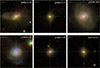Fig. 1.

Sloan Digital Sky Survey gri images of the QSO2s. North is up and east to the left. Horizontal bars in the top-left corner of each image indicate the physical size of 5″. The images are 40″ × 40″ in size.

Table 1.

Main properties of the QSO2s.

3. GTC/EMIR observations and data reduction

The six QSO2s were observed with the NIR multi-slit spectrograph EMIR (Garzón et al. 2006, 2014, 2022) installed at the Naysmith-A focal station of the GTC at the Roque de los Muchachos Observatory in La Palma. EMIR has a 2048 × 2048 Teledyne HAWAII-2 HgCdTe NIR-optimized chip with a pixel size of 0.2″. The observations were carried out in service mode between June 2018 and August 2019 as part of proposals GTC77-18A, GTC62-18B, and GTCMULTIPLE2G-19A (PI: Ramos Almeida). Observing conditions were either clear or spectroscopic. Previous observations taken as part of these programs were published in Ramos Almeida et al. (2019) and Speranza et al. (2022). All spectra were taken with the K-grism, with a nominal dispersion 1.71 Å/pix and resolving power λ/δλ = 4000. The long-slit used has a width of 0.8″. The instrumental width estimated from ArHg, Ne, and Xe arc lamps was ∼6.0 Å (∼82 km s⁻¹). EMIR has a configurable slit unit (CSU) that allows the user to configure and position slits over the 4′ × 6.67′ spectroscopic field of view (FOV). Therefore, depending on the redshift of our targets, we positioned the 0.8″ slit either in the center of the FOV or shifted to the left or right to ensure that the wavelength coverage included the emission lines of interest. Before each QSO2 observation, J-band acquisition images were taken for slit positioning and seeing-determination by measuring the FWHM of several stars in the FOV. The spectra were then taken following a nodding pattern ABBA, with an offset of 30″, for improved sky subtraction. Standard star K-band spectroscopic observations followed each QSO2 (with an exposure time of 4 × 60 s = 240 s) for both flux calibration and telluric absorption correction. Table 2 summarizes the main details of the observations.

The data reduction was done as follows. First, 2D frames were flat fielded using blue and red flats with individual exposures of 1.5 s and 6 s to improve the correction in the blue and red part of the spectra. Bad pixels were masked using the IRAF (Tody 1986, 1993) task ccdmask. The wavelength calibration was done using HgAr, Ne, and Xe arc lamps spectra and the IRAF tasks identify and reidentify. Consecutive pairs of AB and BA frames were subtracted to remove the sky background and then combined with the IRAF package lirisdr to obtain the two-dimensional spectra. We then extracted one-dimensional nuclear spectra of each QSO2 centered at the peak of the continuum emission and using the apertures listed on the last column of Table 2 using the IRAF package apextract. These apertures were chosen based on the seeing FWHM measured from stars present in the J-band acquisition images of the QSO2s, which range between 0.8 and 1.4″. At the redshift of the QSO2s, this corresponds to the central 1.0–3.2 kpc of the galaxies. For J1713+57, the nuclear spectrum is the combination of the two one-dimensional spectra obtained from the data of two different nights (see Table 2).

Flux calibration was performed by fitting the continuum of the standard star observed just after each QSO2, and comparing them to their known integrated magnitude in the K-band, making use of IRAF tasks standard, sensfunc, and calibrate. Telluric absorption correction was done using the standard star spectrum and the IRAF task telluric, although for some of the targets the sky transmission was modeled instead using the ESO tool SKYCALC (Noll et al. 2012; Jones et al. 2013; Moehler et al. 2014). The nuclear spectra of the six QSO2s are shown in Fig. 2.

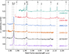Fig. 2.

EMIR K-band nuclear spectra of the QSO2s showing the emission lines detected. The spectra were scaled in the Y-axis with the purpose of better visualization and smoothed using a 10-pixel boxcar. The spectra of the QSO2s are displayed from top to bottom in order of increasing redshift. Vertical dashed black lines indicate the position of the atomic lines, and dotted lines indicate the H₂ lines.

Table 2.

Summary of the GTC/EMIR long-slit observations.

4. Methodology and results

4.1. Nuclear spectra

The nuclear spectra of the QSO2s show emission lines tracing different gas phases, from low- to high-ionized gas and warm molecular gas, as shown in Fig. 2. As can be seen from Fig. 2, the spectra of the two QSO2s with the lowest redshifts, J1440+53 and J1034+60 (z = 0.04 and 0.05 respectively) do not include the Paα line but Brγ, and in the case of J1440+53, also H₂ 1-0S(0). The other four QSO2s, which have redshifts between 0.08 and 0.13, include Paα. Helium lines, such as He II λ1.8637 μm, He I λ1.8691 μm, and He I λ2.0587 μm are also detected for some sources. Furthermore, the coronal emission line of [Si VI] λ1.963 μm with ionization potential χ_e = 167 eV (Oliva & Moorwood 1990; Ramos Almeida et al. 2006; Mazzalay et al. 2013) is ubiquitous in our sample and it is the second most prominent emission line in the spectra of the QSO2s, after Paα. All QSO2s present H₂ emission lines in their spectra, which trace molecular gas at T > 1000 K. We detect H₂ lines from 1-0S(1) to S(4) in all the QSO2s, also S(0) in J1440+53, and S(5) in J0802+25, J1455+35, and J1713+57.

To quantify the ionized and warm molecular gas kinematics and fluxes we fit the emission line profiles using Gaussians, as shown in Fig. 3 for J1440+53. We fit a first-order polynomial function to two continuum bands blue- and red-ward of the emission lines. Then we modeled the emission line profiles with single or multiple Gaussian components using an in-house developed code (Speranza et al. 2022, 2024; Musiimenta et al. 2024) that makes use of the Astropy python library (Astropy Collaboration 2022). The fits are shown in Figs. 3 and A.1–A.6. Tables A.1–A.6 list the FWHM, velocity shift, flux, and flux fraction of each of the Gaussian components fit to the emission lines. The velocity shift is relative to the central wavelength of the narrow component fit to the Paα/Brγ profiles. When two narrow components are fit instead, the velocity shifts are relative to the amplitude weighted value of the central wavelengths of the two narrow components. The flux uncertainties are the quadratic sum of the fit uncertainty obtained from Monte Carlo simulations and the flux calibration error estimated using the standard stars (average flux calibration error of 26%). In addition, since the emission lines were measured in the rest frame, a multiplicative factor of (1 + z) was applied to the fluxes.

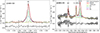Fig. 3.

Examples of emission line fits. The rest-frame spectrum of J1440+53 and residuals are shown in black, and the fit model is in red. Narrow (n), intermediate (i), and broad (b) components are shown in green, blue, and magenta. The spectra were smoothed using a 4-pixel boxcar, and residuals were scaled up from zero to reduce blank space. Vertical dotted lines correspond to the peak of the narrow component fit to each line.

Since some of the NIR emission lines present complex kinematics, are blended (e.g., [Si VI] and H₂ 1-0S(3), and/or they have relatively low signal-to-noise), we performed optical emission line fits using the available optical Sloan Digital Sky Survey (SDSS, York et al. 2000; Abazajian et al. 2009) spectra of the QSO2s to use them as reference for the NIR fits, following Ramos Almeida et al. (2019) and Speranza et al. (2022). The criteria to decide the number of Gaussian components needed to fit the optical lines was 1) an improvement of ≥10% in the reduced χ², following Bessiere et al. (2024) and Speranza et al. (2024), and 2) line fluxes representing ≥10% of the total emission line flux. We then fit the NIR lines using the same number of Gaussian components as in the optical, and the optical kinematics as initial values. Hβ was often used as a reference for Paα, Brγ, He I, and He II since they must follow similar kinematics. For Brδ, either Paα/Brγ or Hβ were considered, and [OIII] λ5007 Å was used as reference for [Si VI]. For fitting H₂ 1-0S(3), that is blended with [Si VI], the fit of H₂ 1-0S(1) was taken as reference. Exceptions to the previous are described in Tables A.1–A.6.

For the warm molecular lines that are not blended, no initial parameters were considered. In all cases, only one Gaussian component of FWHM ∼ 120–460 km s⁻¹ was enough to reproduce the H₂ line profiles. The velocity shifts that we measured for these components, relative to the narrow component(s) fit to either Paα or Brγ, go from −130 to 60 km s⁻¹. In the case of the atomic lines (i.e., either Paα or Brγ, and [Si VI]), we fit narrow components of FWHM < 600 km s⁻¹ (see Table 3). Two narrow components instead of one were needed to reproduce the profiles of J1034+60, J1440+53, and J1713+57. For all QSO2s but J1034+60, we also fit intermediate components. These components are ≥160 km s⁻¹ broader than the narrowest component fit to a given QSO2, and narrower than the broadest component (see Table 3). Finally, broad components (b) with FWHM ≥ 1200 km s⁻¹ and showing blueshifts of up to −600 km s⁻¹ were fit to all the QSO2s. The parameters derived from the individual fits are shown in Tables A.1–A.6.

Table 3.

Ranges of velocity shifts and FWHMs measured for the different components fit to the atomic lines.

In this work we assume that the narrow components, which exhibit velocities typical of galactic rotation, are tracing gas within the narrow-line region. Since the intermediate and broad components exhibit velocities and widths that cannot be explained by rotation alone, and considering that these QSO2s have ionized outflows detected in [O III]¹ (Bessiere et al. 2024), we consider them to be associated with outflowing gas. It is important to stress that these broad components are not related to the broad-line region of the AGN since this analysis is restricted to a sample of obscured (type-2) AGN, and the intermediate and broad components are detected in both the permitted and forbidden emission lines. The fraction of flux in the outflow components (i.e., adding the flux of the intermediate and broad components, when both are present) is larger than that in the narrow component, with the exception of J0802+25. This is common in the case of QSO2s (Ramos Almeida et al. 2017, 2019; Speranza et al. 2022; Hervella Seoane et al. 2023; Villar Martín et al. 2023; Zanchettin et al. 2025).

4.2. Outflow properties

From the analysis described in Section 4.1 and following our criteria to identify outflows, we find ionized outflows in all six QSO2s, both in the recombination lines and [Si VI]. Outflow components are not found in the H₂ emission lines. The following sections are focused on estimating the corresponding outflow properties, to infer their energetic output, whether there is a connection between the outflows found at different ionization levels, and their potential impact on the host galaxies. As previously mentioned, components (i) and (b) are considered outflow, and the derived outflow properties take both components into account. To estimate the outflow masses (M_out), mass outflow rates (Ṁ_out), and kinetic powers (Ė_kin), we need the fluxes and kinematics measured from the nuclear spectra and reported in Tables A.1–A.6, electron densities (n_e), and outflow extents (r_out).

4.2.1. Electron densities

Electron density (n_e) and temperature (T_e) are important indicators of the physical conditions of the ionized gas, and the former is essential to determining its mass. Moreover, n_e is one of the largest sources of uncertainty for ionized gas masses, potentially leading to orders of magnitude uncertainties on measured values (Harrison et al. 2018; Rose et al. 2018; Davies et al. 2020; Holden et al. 2023; Holden & Tadhunter 2023; Speranza et al. 2024). Here we estimate n_e using two distinct methods.

The first method uses the n_e-sensitive [SII] λλ6716,6731 Å doublet in combination with the T_e-sensitive lines of [OIII] λ4363 Å and [OIII] λ5007 Å (Osterbrock & Ferland 2006). This method (hereafter [SII] method) is sensitive to electron densities in the range $10^{2} \leq log n_{e} \leq 10^{3.5} {cm}^{- 3}$ $Mathematical equation: $ 10^{2} \le \log\ \mathrm{n}_{\mathrm{e}} \le 10^{3.5}\,\mathrm{cm}^{-3} $$ (Rose et al. 2018). The emission line fluxes of the [SII] and [OIII] lines were measured from the stellar continuum-subtracted SDSS spectra of the QSO2s from Bessiere et al. (2024), adopting one Gaussian component to reproduce each emission line. Since [OIII] λ4363 Å is faint and blended with the much brighter Hγ line, we fixed its FWHM to the one obtained for [OIII] λ5007 Å. We then used the emission line ratios as inputs to the python package Pyneb (version 1.1.19; Luridiana et al. 2015), obtaining n_e and T_e using the function getCrossTemDen and the errors from the shaded regions of the diagnostic diagrams generated in Diagnostic, shown in Fig. B.1. We obtain 2.6 $\leq \log n_{e} ({cm}^{- 3}) \leq 3.1$ $Mathematical equation: $ \le \mathrm{{log}\ \mathrm{n}_{\mathrm{e}}\,(\mathrm{cm}^{-3})}\le 3.1 $$ and 12 000 K ≤ T_e ≤ 17 000 K (see Table 4). We note that the line fluxes used to infer n_e and T_e were not corrected for extinction. On average, the impact of applying the extinction correction to the fluxes to derive T_e is ∼1000 − 3000 K. For n_e the difference is much smaller (∼15 cm⁻³) than the measurement errors, since n_e is only weakly dependent on T_e, as shown in the diagnostic diagrams shown in Fig. B.1.

Table 4.

Electron temperatures and densities obtained from the [SII] and TR methods.

The second method consists of using two line ratios that involve trans-auroral lines, namely TR([OII]) = F(3726+3729)/F(7319+7331) and TR([SII]) = F(4068+4076)/F(6716+6731) (hereafter TR method). The [SII] and [OII] line ratios are then compared to a grid of photoionization models generated with Cloudy (Ferland et al. 2013), following the procedure described in Holt et al. (2011), which allows the simultaneous determination of reddening and n_e. This method is sensitive up to much higher n_e than the [SII] method, in the range 2.0 $\leq \log n_{e} ({cm}^{- 3}) \leq$ $Mathematical equation: $ \le \rm{log}\ \mathrm{n}_{\mathrm{e}}\,(\mathrm{cm}^{-3})\le $$ 6.5 (Rose et al. 2018). More details can be found in Sect. 2.4 of Bessiere et al. (2024), from where the corresponding values of n_e were taken. This second method results in electron densities of 3.0 $\leq \log n_{e} ({cm}^{- 3}) \leq$ $Mathematical equation: $ \le {\mathrm{log}\ \mathrm{n}_{\mathrm{e}}\,(\rm{cm}^{-3})}\le $$ 4.1 and reddening values of $0.2 mag \leq E (B - V) \leq 0.4 mag$ $Mathematical equation: $ 0.2\,\mathrm{mag}\le \rm{E(B-V)}\le 0.4\,\mathrm{mag} $$ (see Table 4). Therefore, except in the case of J1034+60, for which we get n_e values consistent within the errors using both methods, the densities measured from the TR method are significantly higher ( $n_{e}^{TR} \sim$ $Mathematical equation: $ \mathrm{n}_{\mathrm{e}}^{\mathrm{TR}} \sim $$ 6– $15 \times n_{e}^{[SII]}$ $Mathematical equation: $ 15\times \mathrm{n}_{\mathrm{e}}^{[\mathrm{SII}]} $$ ) than the ones calculated from the [SII] method.

4.2.2. Outflow extent

To measure the spatial extent of the outflows, we followed the methodology described in Rose et al. (2018) and Ramos Almeida et al. (2019). We built spatial profiles of the blue and red wings of Paα/Brγ and [Si VI] (blue and red shaded areas in the upper panels of Figs. C.1–C.6), avoiding the region covered by the fit narrow component(s) and any other adjacent emission lines. Then we produced an average continuum spatial profile from spatial slices blueward and redward of the broad emission line, and subtracted it from the blue and red broad line profiles. We finally averaged these continuum-subtracted blue and red wing spatial profiles and fit the resulting profile with a Gaussian to measure the outflow radial size (FWHM_out). We also calculate the FWHM of the spatial profile of the narrow component (FWHM_nar) in the same way (green shaded areas in the upper panels of Figs. C.1–C.6). In order to inspect the regions where the broad wings, narrow component, and continuum profiles were extracted, we produce continuum-subtracted maps of the emission lines, shown in the middle panels of Figs. C.1–C.6.

Finally, to investigate whether the outflows are spatially resolved we determined the seeing FWHM (FWHM_seeing) from the K-band spectrum of the corresponding standard star of each QSO2, using λ > 21 000 Å (to avoid telluric absorption) to extract the continuum profile and fit it with a Gaussian. We considered an outflow resolved if its continuum-subtracted profile FWHM is

$\begin{matrix} {FWHM}_{out} > {FWHM}_{seeing} + 3 δ_{seeing}, \end{matrix}$ $Mathematical equation: $$ \begin{aligned} \mathrm{FWHM}_{\rm out} > \mathrm{FWHM}_{\rm seeing} + 3\delta _{\rm seeing}, \end{aligned} $$$ (1)

where FWHM_seeing and δ_seeing are the seeing FWHM and its corresponding error derived from the standard star spatial profile. If we find the outflow to be unresolved, we adopt FWHM_seeing as an upper limit for the outflow extent (r_out). If it is resolved, then we computed the size as

$\begin{matrix} r_{out} = \sqrt{{FWHM}_{out}^{2} - {FWHM}_{seeing}^{2}} . \end{matrix}$ $Mathematical equation: $$ \begin{aligned} \mathrm{r}_{\rm out} = \sqrt{\mathrm{FWHM}_{\rm out}^2-\mathrm{FWHM}_{\rm seeing}^2}. \end{aligned} $$$ (2)

Table 5 shows the seeing FWHM derived from the K-band spectra of the standard stars (FWHM_seeing), the FWHM of the outflow (FWHM_out) and narrow (FWHM_nar) components, and the seeing-deconvolved values (r_out and r_nar). The outflow errors were estimated by adding in quadrature the error propagation of Equation (2) and the standard deviation of five computations of FWHM_out, slightly varying the green, red, blue, and continuum regions shown in Figs. C.1–C.6. From Paα and Brγ we measured outflow extents ranging from 0.3 kpc ≤ r_out ≤ 2.1 kpc. In [Si VI] the outflow is not resolved for J1455+35, J0802+25, and J1440+53. For the other three QSO2s, the [Si VI] outflows have extents of 1.0 kpc ≤ r_out ≤ 2.7 kpc. The outflow extent found for J0945+17 in Paα is 2.13 kpc, which is smaller than 3.37 kpc reported by Speranza et al. (2022) based on integral field data from Gemini/NIFS. This is because those authors measured the outflow extent from 2D outflow flux maps, which are sensitive to fainter structures and probe different position angles, unlike our long-slit data. In fact, Speranza et al. (2022) reported an outflow PA ∼ 125°, where its extent is maximum, and our slit PA is 25°. Finally, for the narrow component, we measure extents that are larger or comparable to the outflow extents within the errors (see Table 5).

Table 5.

Spatial extents of the outflow and narrow components measured from Paα/Brγ and [Si VI].

4.2.3. Outflow energetics

For computing the ionized gas mass in the outflow from the recombination lines, we used either the Paα or Brγ extinction corrected fluxes of their intermediate and broad components to calculate their luminosities (L = 4πD_L²F^corr) and then convert them to Hβ luminosity, assuming Case B recombination and T_e = 10⁴ K (L_Hβ = L_Paα/0.352 and L_Hβ = L_Brγ/0.0281; Osterbrock & Ferland 2006). We performed the extinction correction using the E(B-V) values reported in Table 4, and assumed R_V = 3.1 and the extinction law from Cardelli et al. (1989). Then, following Equation (1) from Rose et al. (2018):

$\begin{matrix} M_{Hion} = \frac{L_{H β} m_{p}}{α_{H β}^{eff} h ν_{H β} n_{e}}, \end{matrix}$ $Mathematical equation: $$ \begin{aligned} \mathrm{M}_{\rm Hion} = \frac{\mathrm{L}_{\mathrm{H}\beta } \mathrm{m}_{\rm p}}{\alpha ^\mathrm{eff}_{\mathrm{H}\beta }\mathrm{h}\nu _{\mathrm{H}\beta }\mathrm{n}_{\rm e}} , \end{aligned} $$$ (3)

where m_p = 8.41 × 10⁻⁵⁸ M_⊙, $α_{H β}^{eff} = 3.03 \times 10^{- 14} {cm}^{3} s^{- 1}$ $Mathematical equation: $ \mathrm{\alpha}^{\mathrm{eff}}_{\mathrm{H}\beta} = 3.03 \,{\times}\, 10^{-14} \,\mathrm{cm}^{3} \,\mathrm{s}^{-1} $$ , and ν_Hβ = 6.167 × 10¹⁴ s⁻¹, with h = 6.626 × 10⁻³⁴ Js, we calculated the total ionized gas mass in the outflow.

For estimating the outflow mass of the coronal [Si VI] emission line, we described its luminosity as

$\begin{matrix} L_{[Si VI]} = \int_{V} f n_{e} n ({Si}^{5 +}) j_{[Si VI]} (n_{e}, T_{e}) dV, \end{matrix}$ $Mathematical equation: $$ \begin{aligned} \mathrm{L}_{[\mathrm {Si\,VI}]} = \int _{\rm V} \mathrm{f} \,\mathrm{n}_{\rm e} \,\mathrm{n}(\mathrm{Si}^{5+}) \,\mathrm{j}_{[\mathrm {Si\,VI}]}(\mathrm{n}_{\rm e},\mathrm{T}_{\rm e}) \,\mathrm{dV}, \end{aligned} $$$ (4)

where f is the filling factor, n(Si⁵⁺) the density of Si⁵⁺, and $j_{[Si VI]}$ $Mathematical equation: $ \mathrm{j}_{[\rm{Si\,VI}]} $$ its emissivity, which is a function of n_e and T_e. The n(Si⁵⁺) can be also defined as

$\begin{matrix} n ({Si}^{5 +}) = [\frac{n ({Si}^{5 +})}{n (Si)}] [\frac{n (Si)}{n (H)}] [\frac{n (H)}{n_{e}}] n_{e} . \end{matrix}$ $Mathematical equation: $$ \begin{aligned} \mathrm{n}(\mathrm{Si}^{5+}) = \left[\frac{\mathrm{n}(\mathrm{Si}^{5+})}{\mathrm{n}(\mathrm{Si})}\right]\left[\frac{\mathrm{n}(\mathrm{Si})}{\mathrm{n}(\mathrm{H})}\right]\left[\frac{\mathrm{n}(\mathrm{H})}{\mathrm{n}_{\rm e}}\right]\mathrm{n}_{\rm e}. \end{aligned} $$$ (5)

Following Carniani et al. (2015) and Belli et al. (2024), we assume that the Si⁵⁺ is dominant over neutral n(Si⁵⁺)/n(Si) = 1. As in Carniani et al. (2015) we can assume n(H)/n_e = (1.2)⁻¹, as n_e ≈ n(H)+2 × n(He) = n(H) + 2 × 0.1 × n(H) = 1.2 × n(H) when we consider 10% of helium atoms. Then, using Equation (3) in Carniani et al. (2015), we can write

$\begin{matrix} L_{[Si VI]} = {(1.2)}^{- 1} j_{[Si VI]} (n_{e}, T_{e}) ⟨ n_{e}^{2} ⟩ {(\frac{n (Si)}{n (H)})}_{⊙} 10^{[Si / H] - {[Si / H]}_{⊙}} f V, \end{matrix}$ $Mathematical equation: $$ \begin{aligned} \mathrm{L}_{[\mathrm {Si}\,\mathrm {VI}]} = (1.2)^{-1}\,\mathrm {j}_{[\mathrm {Si}\,\mathrm {VI}]}(\mathrm{n}_{\rm e},\mathrm{T}_{\rm e}) \,\langle \mathrm{n}_{\rm e}^2 \rangle \, \left(\frac{{{\mathrm n}(\mathrm {Si})}}{{\mathrm n(\mathrm H)}}\right)_{\odot } 10^{[\mathrm{{Si}/\mathrm {H}}]-[\mathrm {{Si}/\mathrm {H}}]_{\odot }} \, \mathrm {f} \,\mathrm {V}, \end{aligned} $$$ (6)

and based on Equation (4) of the same paper,

$\begin{matrix} M_{[Si VI]} \approx 1.06 m_{p} ⟨ n_{e} ⟩ f V . \end{matrix}$ $Mathematical equation: $$ \begin{aligned} \mathrm{M}_{[\mathrm {Si}\,\mathrm {VI}]} \approx 1.06 \, \mathrm{m}_{\rm p} \,\langle \mathrm{n}_{\rm e} \rangle \, \mathrm {f} \, \mathrm {V}. \end{aligned} $$$ (7)

Connecting Equations (6) and (7) using $f V$ $Mathematical equation: $ \mathrm{f} \, \rm{V} $$ , assuming that ⟨n_e²⟩=⟨n_e⟩², we obtained

$\begin{matrix} M_{[Si VI]} \approx \frac{1.4 L_{[Si VI]} m_{p}}{n_{e} j_{[Si VI]} {(\frac{n (Si)}{n (H)})}_{⊙} 10^{[Si / H] - {[Si / H]}_{⊙}}} \cdot \end{matrix}$ $Mathematical equation: $$ \begin{aligned} \mathrm{M}_{[\mathrm {Si}\,\mathrm {VI}]} \approx \frac{1.4 \, \mathrm {L}_{[\mathrm {Si\,VI}]} \, \mathrm{m}_{\rm p}}{{\mathrm n}_{\rm e} \, \mathrm {j}_{[\mathrm {Si\,VI}]} \, \left(\frac{{\mathrm n(\mathrm{Si})}}{{\mathrm n( \mathrm H)}}\right)_{\odot } 10^{[\mathrm {Si/H}]-[\mathrm {Si/H}]_{\odot }}}\cdot \end{aligned} $$$ (8)

Using Chianti IDL 10.1 (Dere et al. 1997; Del Zanna et al. 2021) we obtain the emissivities (dividing EMISS_CALC output by n_e) for the mean [SII] and TR methods electron densities found in the sample: $j_{[Si VI]} (T_{e} = 10^{4} K, n_{e} = 752 {cm}^{- 3}) = 2.4772 \times 10^{- 21} erg s^{- 1} {cm}^{3}$ $Mathematical equation: $ \mathrm{j}_{[\rm{Si}\,\rm{VI}]}(\mathrm{T}_{\mathrm{e}} = 10^4\,\rm{K}, \mathrm{n}_{\mathrm{e}} = 752\,\rm{cm}^{-3}) = 2.4772 \times 10^{-21}\,\rm{erg}\,\rm{s}^{-1} \,\mathrm{cm}^{3} $$ and $j_{[Si VI]} (T_{e} = 10^{4} K, n_{e} = 5741 {cm}^{- 3}) = 2.4828 \times 10^{- 21} erg s^{- 1} {cm}^{3}$ $Mathematical equation: $ \mathrm{j}_{[\rm{Si}\,\rm{VI}]}(\mathrm{T}_{\mathrm{e}} = 10^4\,\rm{K}, \mathrm{n}_{\mathrm{e}} = 5741\,\rm{cm}^{-3}) = 2.4828 \times 10^{-21}\,\rm{erg}\,\rm{s}^{-1}\,\rm{cm}^{3} $$ . Since there is no significant variation in the derived emissivities, we adopted the value of $j_{[Si VI]} = 2.48 \times 10^{- 21} erg s^{- 1} {cm}^{3}$ $Mathematical equation: $ \mathrm{j}_{[\rm{Si\,VI}]} = 2.48\times 10^{-21}\,\rm{erg}\,\rm{s}^{-1}\,\rm{cm}^{3} $$ . Furthermore, we adopted the solar Si abundance² from Asplund et al. (2021) as log(ϵ_Si) = 7.51 and considering that $\log (ϵ_{Si}) = log ([\frac{n (Si)}{n (H)}]) + 12$ $Mathematical equation: $ \mathrm{log}(\epsilon_\mathrm{{Si}}) = \log\left(\left[\frac{{\mathrm n(\mathrm{Si})}}{{\mathrm n(\mathrm H)}}\right]\right) + 12 $$ , we find $[\frac{n (Si)}{n (H)}] = 3.2359 \times 10^{- 5}$ $Mathematical equation: $ \left[\frac{{\mathrm {n(Si)}}}{{\mathrm n(\mathrm H)}}\right] = 3.2359 \times 10^{-5} $$ . Assuming the values of emissivity and solar Si abundance described above, and m_p = 8.41 × 10⁻⁵⁸ M_⊙, we obtained the [Si VI] mass as

$\begin{matrix} M_{[Si VI]} = 1.415 \times 10^{- 32} \frac{L_{[Si VI]}}{n_{e}} M_{⊙} . \end{matrix}$ $Mathematical equation: $$ \begin{aligned} \mathrm{M}_{[\mathrm {Si\,VI}]} = 1.415\, {\times } \,10^{-32} \, \frac{{\mathrm L}_{[\mathrm {Si\,VI}]}}{{\mathrm n}_{\rm e}} \, \mathrm {M}_{\odot }. \end{aligned} $$$ (9)

The corresponding outflow masses calculated from Paα/Brγ and [Si VI] are reported in Table D.2. We find ionized gas masses of M_Hion = 0.08−20 × 10⁶ M_⊙ from the recombination lines and of m_[Si VI] = 0.02−2 × 10⁶ M_⊙ from [Si VI] when assuming TR-method electron densities. When assuming [SII]-method electrons densities we obtain ionized gas masses of m_Hion = 0.5−33 × 10⁶ M_⊙ from the recombination lines and of m_[Si VI] = 0.1−4 × 10⁶ M_⊙ from [Si VI]. Then, to compute the mass outflow rates, we assumed spherical geometry for the outflow, following Fiore et al. (2017),

$\begin{matrix} {\dot{M}}_{out} = 3 v_{out} \frac{M_{out}}{r_{out}}, \end{matrix}$ $Mathematical equation: $$ \begin{aligned} \dot{\mathrm{M}}_{\rm out} = 3 \, \mathrm {v}_{\rm out} \, \frac{{\mathrm M}_{\rm {out}}}{{\mathrm r}_{\rm {out}}}, \end{aligned} $$$ (10)

and we followed the kinetic power definition from Hervella Seoane et al. (2023):

$\begin{matrix} {\dot{E}}_{kin} = \frac{{\dot{M}}_{out}}{2} \times v_{out}^{2} . \end{matrix}$ $Mathematical equation: $$ \begin{aligned} \dot{\mathrm{E}}_{\rm kin} = \frac{\dot{\mathrm{M}}_{\rm out}}{2} \times \mathrm {v}_{\rm out}^2. \end{aligned} $$$ (11)

From these properties, we have also calculated the coupling efficiency as ξ = Ė_kin/L_Bol and the mass loading factor $η = {\dot{M}}_{out} / SFR$ $Mathematical equation: $ \mathrm{\eta} = \dot{\mathrm{{M}}}_\mathrm{{out}}/\rm{SFR} $$ . Since the measured velocity shifts (v_s) are projected velocities, besides using $v_{out} = v_{s}$ $Mathematical equation: $ \mathrm{v}_{\mathrm{out}} = \rm{v}_{\mathrm{s}} $$ to infer the outflow properties, we also computed their upper limits adopting the maximum outflow velocity $v_{\max} = | v_{s} | + 2 σ$ $Mathematical equation: $ \mathrm{v}_\mathrm{{max}} = |\rm{v}_\mathrm{{s}}| + 2\sigma $$ (i.e., to account for projection effects, we measured the velocity in the wing of the line, under the assumption that this corresponds to the velocity of the gas moving directly toward us; Rupke & Veilleux 2013; Fiore et al. 2017; Speranza et al. 2022), where $σ \sim FWHM / 2.355$ $Mathematical equation: $ \sigma \sim \rm{FWHM}/2.355 $$ . Table D.1 shows the observed outflow properties (e.g., n_e, r_out, v_s, v_max) directly measured from the spectra, while Table D.2 summarises the derived outflow properties (e.g., M_out, Ṁ_out, Ė_kin, ξ, η) using the electron densities estimated with the two methods here considered. The properties have been calculated separately for each outflow component (i.e., b and i, if present) and then added. Assuming the TR-method electron densities we estimate mass outflow rates of Ṁ_Hion ∼ 0.03−6 M_⊙ yr⁻¹ from the recombination lines and of Ṁ_[Si VI] ∼ 0.004−1 M_⊙ yr⁻¹ from [Si VI]. Their kinetic powers are Ė_Hion ∼ 10^37.8−40.8 erg s⁻¹ for recombination lines and Ė_[Si VI] ∼ 10^36.6−40.5 erg s⁻¹ for [Si VI]. If instead we assume [SII]-method electron densities the recombination lines mass outflow rates are Ṁ_Hion ∼ 0.2−10 M_⊙ yr⁻¹ and from [Si VI] of Ṁ_[Si VI] ∼ 0.02−2 M_⊙ yr⁻¹. The corresponding kinetic powers are Ė_Hion ∼ 10^38.6−41.6 erg s⁻¹ for recombination lines and Ė_[Si VI] ∼ 10^37.4−41.3 erg s⁻¹ for [Si VI].

5. Discussion

Here we discuss the results of our study of the ionized and warm molecular gas properties of six nearby QSO2s. In Sections 5.1 and 5.3 we focus on the ionized gas outflow properties derived using TR-based electron densities instead of the [SII]-based ones, as the findings of recent studies indicate that ionized outflows exhibit higher electron densities than non-outflowing gas (Speranza et al. 2022; Holden et al. 2023). Since the TR lines are sensitive to higher densities than [SII], they are more appropriate for calculating the properties of ionized outflows (see Holden et al. 2026). In addition, the electron densities derived from the mid-infrared coronal lines of [NeV] detected in JWST observations of five QSO2s in the QSOFEED sample are in good agreement with those obtained from the TR-method and higher than those from the [SII]-method (Ramos Almeida et al. 2025).

5.1. Energetics of the ionized outflows in QSO2s

Here we have characterized the ionized gas outflows of the QSO2s by means of their Paα or Brγ emission lines, which are less affected by obscuration than the optical emission lines. To investigate whether these NIR emission lines provide different outflow properties than those obtained from optical lines (e.g., Hβ and [OIII]), in Table 6 we compare them with those measured for the same six QSO2s and for the whole QSOFEED sample of 48 QSO2s, but using optical SDSS spectra. For these QSO2s, Bessiere et al. (2024) measured the ionized outflow properties using a non-parametric analysis of the [OIII] λ5007 Åemission line, considering TR-based densities, and assuming an outflow extent of r_out = 0.62 kpc. The [OIII] masses were multiplied by three in order to estimate the total ionized gas masses ( $M_{Hion} \sim 3 \times M_{[OIII]}$ $Mathematical equation: $ \mathrm{M}_{\mathrm{Hion}} \sim 3\times \mathrm{M}_{[\rm{OIII}]} $$ ; Fiore et al. 2017).

Table 6.

Comparison between the outflow properties of different samples of QSO2s.

Focusing first on the ionized outflow properties of the six QSO2s studied here, we measure higher outflow masses from the NIR recombination lines, with median $\log (M_{Hion} [M_{⊙}]) = 5.81$ $Mathematical equation: $ \mathrm{log}(\rm{M}_\mathrm{{Hion}}\,[\rm{M}_{\odot}]) = 5.81 $$ , than Bessiere et al. (2024), who reported median $\log (M_{Hion} [M_{⊙}]) = 4.91$ $Mathematical equation: $ \mathrm{log}(\rm{M}_\mathrm{{Hion}}[\rm{M}_{\odot}]) = 4.91 $$ for the same targets (i.e., 7.9 times lower than our median measurement; see Table 6). The largest difference that we found is between the NIR and optical outflow masses measured for J1034+60 ( $\log (M_{Hion} [M_{⊙}]) = 7.30$ $Mathematical equation: $ \mathrm{log}(\rm{M}_\mathrm{{Hion}}\,[\rm{M}_{\odot}]) = 7.30 $$ here versus $\log (M_{Hion} [M_{⊙}]) = 5.59$ $Mathematical equation: $ \mathrm{log}(\rm{M}_\mathrm{{Hion}}\,[\rm{M}_{\odot}]) = 5.59 $$ in Bessiere et al. (2024). This is due to the large integrated flux of the broad component fit to Brγ (78% of the total flux in the line; see Table A.3 and Fig. A.3). Part of these differences can be accounted for by the different fitting techniques employed in the two works, i.e., parametric versus non-parametric. Hervella Seoane et al. (2023) reported parametric-based median M_Hion values 3.4 times higher than the non-parametric ones measured for the same targets. This happens because the parametric analysis considers the integrated flux of the broad and intermediate components fit to the line profiles, while non-parametric methods just use the integrated flux of the high-velocity wings of the lines. This, together with the relatively large flux calibration uncertainty of the NIR fluxes (see Section 4.1), explains part of the difference between the optical and NIR masses of the same targets. Finally, it is also possible that the NIR data, less affected by extinction than optical spectra and probing a smaller physical region (seeing limited versus 3″ SDSS fiber size), allow us to peer deeper in the outflow regions, recovering part of the flux that remains undetected in the optical (Ramos Almeida et al. 2017).

The NIR and optical mass outflow rates (Ṁ_Hion) are consistent within the errors, having median values of 0.6 and 0.35 M_⊙ yr⁻¹ respectively. This happens because the higher NIR outflow masses are compensated by 1) the lower NIR outflow velocities that we measure from the parametric method, compared to those derived from the non-parametric analysis (see Hervella Seoane et al. 2023 for a comparison of the outflow mass rates derived from different methods) and 2) by the larger outflow radii that we used as compared to the fix value of 0.62 kpc used by Bessiere et al. (2024)³.

The lower NIR outflow velocities that we measured from our parametric fits also result in lower kinetic energies (Ė_Hion) and coupling efficiencies (ξ_Hion) than those derived from optical data by Bessiere et al. (2024) (median values of log(Ė_Hion [erg s⁻¹]) = 40.2 and ξ_Hion = 0.0004% in the NIR and 41.1 and 0.003% in the optical), as ${\dot{E}}_{Hion} \propto v_{out}^{3}$ $Mathematical equation: $ \dot{\mathrm{E}}_{\mathrm{Hion}}\propto \mathrm{v}_{\mathrm{out}}^3 $$ . Hervella Seoane et al. (2023) reported even larger differences between the kinetic energies derived from the parametric and non-parametric analysis of the same targets.

Our results suggest that, at least for the QSO2s studied here, there are no significant variations between the NIR and optical outflow mass rates and kinetic energies if we account for the different methodologies used to characterize the physical outflow properties. However, the outflow masses that we measure in the NIR are 7.9 times higher than the optical ones, considering median values. This is partly due to the use of a parametric method to fit the NIR lines and to the flux calibration uncertainty of the NIR spectra, and possibly to the higher angular resolution and lower reddening of the NIR data as well, which allow us to probe deeper outflow regions. The outflow properties of the six QSO2s studied here are representative of the whole QSOFEED sample looking at the median values and ranges of the different outflow properties reported in Table 6.

We can also compare our outflow energetics with those obtained from the parametric analysis of the [OIII] line of 18 QSO2s at z = 0.3–0.41 observed with the Gemini South Telescope (Hervella Seoane et al. 2023). The authors also assumed $M_{Hion} \sim 3 \times M_{[OIII]}$ $Mathematical equation: $ \mathrm{M}_{\mathrm{Hion}} \sim 3\times \rm{M}_{[\rm{OIII}]} $$ . This sample of QSO2s have $\log (L_{bol} [{erg s}^{- 1}]) = 44.9 - 46.7$ $Mathematical equation: $ \mathrm{log}(\rm{L}_\mathrm{{bol}}[\rm{erg\,s}^{-1}]) = 44.9{-}46.7 $$ , with a median value of 45.5, coinciding with the median bolometric luminosity of our subset of six QSO2s. Their outflow extent assumption, of 1 kpc, agrees well with our measurements (median r_out = 1.1 kpc). Since, they assumed $n_{e} = 200 {cm}^{- 3}$ $Mathematical equation: $ \mathrm{n}_{\mathrm{e}} = 200\,\mathrm{cm}^{-3} $$ , we multiplied their outflow masses by that value of n_e, and divided them by the median value of the QSOFEED sample measured with the TR-based method, which is $n_{e} = 2570 {cm}^{- 3}$ $Mathematical equation: $ \mathrm{n}_{\mathrm{e}} = 2570\,\mathrm{cm}^{-3} $$ (Bessiere et al. 2024). We did this to make their ionized outflow properties comparable to ours. The outflow masses measured for the two samples have medians of log( $M_{Hion} [M_{⊙}]$ $Mathematical equation: $ \mathrm{M}_{\mathrm{Hion}}[\rm{M}_{\odot}] $$ ) = 5.81 and 5.35 at z = 0.1 and z = 0.3–0.41, respectively (2.9 times higher in the case of the low-z QSO2s). The outflow mass rates and kinetic powers are also lower in the case of the QSO2s at z = 0.3–0.41, with medians of 0.14 M_⊙ yr⁻¹ and log(Ė_Hion [erg s⁻¹]) = 39.2, but they span similar ranges: log(Ė_Hion [erg s⁻¹]) ∼ 37–41 at z = 0.3–0.41 and ∼38–41 at z = 0.1. Overall, this comparison suggests that there is no significant evolution in the outflow properties of QSO2s from redshift z = 0.1 and z = 0.3–0.41, albeit the samples are small.

Finally, we compared our outflow energetics with those of QSO2s at higher redshifts based on data of the JWST Near Infrared Spectrograph (NIRSpec). Bertola et al. (2025) and Perna et al. (2025) reported outflow properties from Hα observations of four QSO2s at z ∼ 2.05–3.51 and log L_bol = 45.2–46.2 (see Table 6). Both studies used fixed electron density values and used different definitions of outflow velocity. In order to compare to our results, we corrected their outflow properties values assuming $n_{e} = 2570 {cm}^{- 3}$ $Mathematical equation: $ \mathrm{n}_{\mathrm{e}} = 2570\,\mathrm{cm}^{-3} $$ and v_out = v_s (see Table 6). The median values of log M_Hion and Ṁ_Hion of the high-redshift QSO2s are 31 and 10 times higher than those of the six low-redshift QSO2s studied here, but the median kinetic power is only a factor 1.3 higher (see Table 6). It is also noteworthy that two of the high-z QSO2s have $\log (M_{Hion} [M_{⊙}]) = 5.8$ $Mathematical equation: $ \mathrm{log}(\rm{M}_{\mathrm{Hion}}[\mathrm{M}_{\odot}]) = 5.8 $$ –6.4 and Ṁ_Hion = 0.2–0.7 M_⊙ yr⁻¹, which are similar to the properties of the local QSO2s. Despite the small number of targets involved in this comparison, the outflow masses and mass outflow rates of QSO2s at z ∼ 2–3.5 are higher than those of local QSO2s, but their kinetic powers are comparable.

5.2. Scaling relations

In Fig. 4 we show the relation between mass outflow rate and bolometric luminosity. Our data points correspond to the mass outflow rates derived from the hydrogen recombination lines (either Paα or Brγ), using $v_{out} = v_{s}$ $Mathematical equation: $ \mathrm{v}_\mathrm{{out}} = \rm{v}_{\mathrm{s}} $$ and TR-based electron densities. In Fig. 4 we also include the mass outflow rates of AGN and ULIRGs at z < 0.5 from Fiore et al. (2017). These were calculated assuming n $_{e} = 200 {cm}^{- 3}$ $Mathematical equation: $ _{\mathrm{e}} = 200\,\mathrm{cm}^{-3} $$ , v_out = v_max, and r_out = 1 kpc, and using Hα, Hβ, or [OIII] (assuming $M_{Hion} ≃ M_{H β} ≃ 3 \times M_{[OIII]}$ $Mathematical equation: $ \mathrm{M}_{\mathrm{Hion}} \simeq \rm{M}_\mathrm{{H}\beta} \simeq 3\times \rm{M}_{[\rm{OIII}]} $$ ). Therefore, we divided the Fiore et al. (2017) mass outflow rates by 130 (2.1 dex) to account for the differences in how their outflow velocity was measured relative to ours, and to avoid assuming an electron density based on [SII] measurements, which are sensitive to $n_{e} \sim 100 - 3000 {cm}^{- 3}$ $Mathematical equation: $ \mathrm{n}_{\mathrm{e}}\sim100{-}3000\,\mathrm{cm}^{-3} $$ (we refer the reader to Speranza et al. 2024 and Holden et al. 2026 for a discussion on the influence of electron density on the mass outflow rates). This value of 130 comes from first converting from $v_{out} = v_{\max}$ $Mathematical equation: $ \mathrm{v}_{\mathrm{out}} = \rm{v}_\mathrm{{max}} $$ to $v_{out} = v_{s}$ $Mathematical equation: $ \mathrm{v}_\mathrm{{out}} = \rm{v}_{\mathrm{s}} $$ , using the ratio of the median values reported in Hervella Seoane et al. (2023), of ∼10 (1.0 dex). We then converted from $n_{e} = 200 {cm}^{- 3}$ $Mathematical equation: $ \mathrm{n}_{\mathrm{e}} = 200\,\mathrm{cm}^{-3} $$ to $n_{e} = 2570 {cm}^{- 3}$ $Mathematical equation: $ \mathrm{n}_{e} = 2570\,\mathrm{cm}^{-3} $$ , dividing the mass rates by ∼13 (1.1 dex)⁴. After doing this, the values from Fiore et al. (2017) are similar to ours, showing the strong influence of methodology and assumptions on the outflow mass rate determination (Hervella Seoane et al. 2023; Harrison & Ramos Almeida 2024). We also included the mass outflow rates of another four QSO2s from the QSOFEED sample (Speranza et al. 2024). They were calculated from [OIII] observations obtained with the integral field unit of GTC/MEGARA, using a non-parametric analysis, and TR-based electron densities. Probably because of the non-parametric analysis and the better sensitivity and spatial coverage of the optical IFU data, their mass outflow rates are among the highest in Fig. 4.

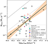Fig. 4.

Relation between Ṁ_Hion and L_bol. Turquoise points are our ionized mass outflow rates (Ṁ_Hion), calculated from either Paα or Brγ and using TR-based electron densities. Data of other QSO2s are shown with different colors and symbols. Open squares are mass outflow rates from Fiore et al. (2017), divided by 130 (see text). The dashed and dotted gray lines are the scaling relations from Fiore et al. (2017) and Davies et al. (2020), respectively, and the solid black line is the linear fit to all the data points included in the plot. The orange shaded area represents the 1σ confidence interval of the fit.

We also calculated the mass outflow rates of another two QSOFEED QSO2s that were observed in the NIR using VLT/SINFONI observations: J1430+13 and J1356+10. For J1356+10 we used the Paα fluxes and velocity shifts reported in Zanchettin et al. (2025), and the TR-based electron densities and A_V values reported in Ramos Almeida et al. (2025). Since there are no outflow sizes reported for the Paα outflows in Zanchettin et al. (2025), we took the smaller [OIII] outflow radius reported by Speranza et al. (2024) for J1356+10. For J1430+13 we used the Paα fluxes, velocity shifts, and outflow sizes from Ramos Almeida et al. (2017), adopting the TR-based electron density and extinction from Bessiere et al. (2024). Finally, we added the Paα outflow mass rate reported by Ramos Almeida et al. (2019) for the QSO2 J1509+04, which was observed with GTC/EMIR and whose outflow properties were calculated using the same methodology as here. Fig. 4 shows that the QSO2s studied here occupy the same locus as the other QSO2s with NIR measurements. Considering all the data points shown in Fig. 4 with $L_{bol} \sim 10^{45 - 46} {erg s}^{- 1}$ $Mathematical equation: $ \mathrm{L}_{\mathrm{bol}}\sim 10^{45-46}\,\rm{erg\,s}^{-1} $$ , the mass outflow rates are clustered between $0.01 M_{⊙} {yr}^{- 1}$ $Mathematical equation: $ 0.01\,\rm{M}_{\odot}\,\rm{yr}^{-1} $$ and $2 M_{⊙} {yr}^{- 1}$ $Mathematical equation: $ 2\,\rm{M}_{\odot}\,\rm{yr}^{-1} $$ , with the exception of J1034+60. Finally, if we fit all the data points included in Fig. 4 we derive a scaling relation that is 2.6 times lower than that derived by Davies et al. (2020) from a sample of 291 type-II AGN with 43.0 < $\log (L_{bol} [{erg s}^{- 1}])$ $Mathematical equation: $ \mathrm{log}(\rm{L}_\mathrm{{bol}}\,[\rm{erg\,s}^{-1}]) $$ < 48.0. The higher mass outflow rates reported in Davies et al. (2020) arise from their definition of outflow velocity, which is $v_{out} \sim 3 \times v_{s}$ $Mathematical equation: $ \mathrm{v}_\mathrm{{out}} \sim 3\times \rm{v}_{\mathrm{s}} $$ (Baron & Netzer 2019).

5.3. Coronal line outflows

The QSO2s studied here show [Si VI] outflows with similar kinematics and radii as those measured from the recombination lines. The outflow extents reported for [Si VI] outflows range from tens to hundreds of parsecs in Seyfert galaxies (Müller-Sánchez et al. 2011; Rodríguez-Ardila et al. 2017; May et al. 2018) and ∼1 kpc in QSO2s (Ramos Almeida et al. 2017, 2019; Speranza et al. 2022; Villar Martín et al. 2023). Despite the small statistics, recent results including ours suggest that coronal line outflows in QSO2s show similar extents as those detected in the recombination lines. The outflow physical properties measured from [Si VI] when adopting the TR-based electron densities are Ṁ_[Si VI] ∼ 0.004−1.2 M_⊙ yr⁻¹ and Ė_[Si VI] ∼ 10^36.5−40.5 erg s⁻¹ (see Table D.2). When we consider the velocity of the outflow as v_max we find Ṁ_{[Si VI],max} ∼ 0.08−9.3 M_⊙ yr⁻¹ and Ė_{[Si VI],max} ∼ 0.05−6 × 10⁴² erg s⁻¹. Comparing our findings with the literature is not straightforward, since the few works that computed these quantities were restricted to LLAGN and Seyferts, and the method used to estimate those properties did not rely on the flux of the lines. Müller-Sánchez et al. (2011) analysed SINFONI data of seven nearby Seyfert galaxies, detecting [Si VI] outflows and construcing biconical outflow models for them. The mass outflow rates were inferred using their models maximum velocities and lateral surface area, assuming $n_{e} = 5000 {cm}^{- 3}$ $Mathematical equation: $ \mathrm{n}_{\mathrm{e}} = 5000 \,\mathrm{cm}^{-3} $$ and filling factor of f = 0.001. They found [Si VI] mass outflow rates of 4.0–9.0 M_⊙ yr⁻¹ for five galaxies, and 120 M_⊙ yr⁻¹ for NGC 2992. They reported kinetic powers in the range 0.06–5 × 10⁴² erg s⁻¹. Rodríguez-Ardila et al. (2017) studied the Seyfert galaxy NGC 1386 in the K-band with SINFONI and using their measured [Si VI] velocities and angular scales, n_e ∼ 930 cm⁻³ (estimated from the [Ne V] ratio measured with Spitzer), and f = 0.1, they measured a mass outflow rate of 11 M $_{⊙} {yr}^{- 1}$ $Mathematical equation: $ _{\odot}\,\rm{yr}^{-1} $$ and kinetic power of 1.7 × 10⁴¹ erg s⁻¹. May et al. (2018) studied the Seyfert ESO 428-G14, and, using similar assumptions as Rodríguez-Ardila et al. (2017), found mass outflow rates of 3–8 M_⊙ yr⁻¹ and kinetic powers of 2–11 × 10⁴⁰ erg s⁻¹. However, we stress that none of the previously discussed works used the line fluxes to estimate the outflow mass. Here we provide an equation to work out the coronal outflow mass using the line flux.

As in Fiore et al. (2017), where they found that the mass in the Hβ outflows was 3 times those calculated using [OIII], here we attempted to estimate what fraction of the ionized gas mass in the outflow is carried by [Si VI]. Fig. 5 shows the ionized and [Si VI] outflow mass and mass rates, including our six QSO2s and another two with [Si VI] outflow measurements (Ramos Almeida et al. 2017, 2019). The ionized mass outflow rates from the recombination lines, and their corresponding outflow masses, are the same as in Fig. 4. In the case of [Si VI], for J1430+13 we adopted the outflow flux, velocity shift, and radius reported in Ramos Almeida et al. (2017) and the TR-based electron density and reddening from Bessiere et al. (2024). For J1509+34, we use all the measurements in Ramos Almeida et al. (2019) and assumed that the [Si VI] outflow radius is the same as that reported for Paα. For the eight QSO2s, and considering the lower limits as values, $M_{Hion} / M_{[Si VI]} =$ $Mathematical equation: $ \mathrm{M}_{\mathrm{Hion}}/\rm{M}_{[\rm{Si\,VI}]}= $$ [3.0–9.2], with a median of 5.9, and Ṁ_Hion/Ṁ_[Si VI] = [2.4–21.5], with a median of 5.8. In Fig. 5 we also show the linear fits to the data, from which we found a stronger correlation for the outflow mass (Pearson r = 0.97, p-value = 7.0 × 10⁻⁵). These fractions need to be confirmed in larger samples of QSO2s and AGN. Considering this, together with the similar kinematics and extents of the outflows found for [Si VI] and the NIR recombination lines, we conclude that the low- and high-ionization lines are tracing the same outflow events, and not different phenomena (Cicone et al. 2018).

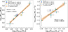Fig. 5.

Total ionized (Hion) versus [Si VI] gas outflow mass (left panel) and mass outflow rate (right panel). Turquoise circles are the QSO2s studied here, with outflow masses and mass rates calculated with TR electron densities, and blue and yellow circles are the QSO2s J1430+13 and J1509+04 from Ramos Almeida et al. (2017, 2019). Solid black lines are the corresponding fits to the data, and the orange shaded area represents the 1σ confidence interval of the fit. The Pearson correlation coefficient and the associated p-value are indicated in each panel.

5.4. The warm molecular gas phase

The six QSO2s studied here were selected because they all showed recombination and H₂ emission lines in the NIR. However, we did not find any outflow associated with the H₂ emission. The same was found for another five QSO2s in the QSOFEED sample using the rotational H₂ lines detected in the nuclear JWST/MIRI spectra (Ramos Almeida et al. 2025). It is noteworthy that the five QSO2s observed with JWST/MIRI show massive outflows of cold molecular gas, detected in CO(2-1) using ALMA observations (Ramos Almeida et al. 2022; Audibert et al. 2025). Nevertheless, recent analysis of deep NIR integral field spectra from VLT/SINFONI of two of these QSO2s, J1430+13 and J1356+10, revealed their elusive warm molecular outflows. These outflows have r_out < 2 kpc and M_out ∼ 2.6 and 1.5 × 10³ M_⊙ (Zanchettin et al. 2025). This indicates that detecting warm molecular outflows is not easy, and indeed, there are only two other QSO2s with warm molecular outflows reported in the literature so far (F08572+3915 NW; Rupke & Veilleux 2013 and J1509+04; Ramos Almeida et al. 2019). This last QSO2, J1509+04, has a NIR H₂ outflow reported, but it appears to lack its MIR counterpart (Ramos Almeida et al. 2025), although further analysis of the MIRI IFU data is required.

Following Speranza et al. (2022), in order to investigate what can be driving the presence or not of warm molecular outflows, we first estimated the H₂ mass of the six QSO2s studied here using the relation from Mazzalay et al. (2013):

$\begin{matrix} M_{H_{2}} \approx 5.0875 \times 10^{13} {(\frac{D_{L}}{Mpc})}^{2} (\frac{F_{H_{2} 1 - 0 S (1)}^{corr}}{{erg s}^{- 1} {cm}^{- 2}}), \end{matrix}$ $Mathematical equation: $$ \begin{aligned} \mathrm{M}_{\rm {H}_2} \approx 5.0875 \times 10^{13} \left(\frac{{\mathrm D}_{\rm L}}{{\mathrm {Mpc}}}\right)^2 \left(\frac{{\mathrm F}_{\rm {H}_2\ 1-0\mathrm {S}(1)}^\mathrm{corr}}{\mathrm{{erg\,s}^{-1}\,\mathrm {cm}^{-2}}}\right), \end{aligned} $$$ (12)

where D_L is the luminosity distance and $F_{H_{2} 1 - 0 S (1)}^{corr}$ $Mathematical equation: $ \mathrm{F}_\mathrm{{H}_2\ 1-0\rm{S}(1)}^{\mathrm{corr}} $$ is the flux measured in $H_{2} 1 - 0 S (1)$ $Mathematical equation: $ \mathrm{H}_2\ 1-0\rm{S}(1) $$ corrected by extinction (see Section 4.2.3 for more details). The H₂ masses are shown in Table 7 together with measurements of other QSO2s reported in the literature.

Table 7.

List of QSO2s with NIR H₂ measurements reported in the literature.

The nuclear H₂ masses of the six QSO2s (i.e., measured from the nuclear spectra shown in Fig. 1) are in the range (0.7–12.9) × 10³ M_⊙. They correspond to regions with sizes of 0.6–3.2 kpc (median of 1.3 kpc). In addition, we also computed H₂ masses from the lines detected in spectra of the central 3″ of the QSO2s (total H₂ masses hereafter, corresponding to scales of 2.1–6.1 kpc, with a median of 4.6 kpc), obtaining values of (1.1–31.9) × 10³ M_⊙.

Using the measurements shown in Table 7, we find that the mean nuclear and total H₂ masses for QSO2s without H₂ outflows are (7.7 ± 3.9) × 10³ M_⊙ and (15.4 ± 9.2) × 10³ M_⊙, while for the four QSO2s with H₂ outflows they are (20.6 ± 18.9) × 10³ M_⊙ and (34.0 ± 15.4) × 10³ M_⊙⁵. Therefore, the mean nuclear (total) H₂ mass in QSO2s with H₂ outflows 2.7 (2.2) times larger than that of QSO2s without H₂ outflows. If confirmed for a larger sample, the nuclear and total warm molecular mass can be relevant factors for driving and/or detecting outflows, but there are counterexamples. For example, J1347+12 (4C12.50) has a higher total H₂ mass than J1356+10, but there is no warm molecular outflow reported for it (Villar Martín et al. 2023), despite the massive cold H₂ molecular outflow detected in high angular resolution CO ALMA observations (Holden et al. 2024). Another example is J0945+17, for which Speranza et al. (2024) reported a total H₂ mass of ∼59 × 10³ M_⊙ measured in the central ∼1″ × 1″ region using Gemini/NIFS data and no outflow detection. It is noteworthy that the discrepancy between the Gemini/NIFS and our GTC/EMIR measurements is likely due to the lower sensitivity of our data to fainter structures (see exposure times in Table 7) and to the fact that we are using long-slit observations along a certain PA, whilst Gemini/NIFS is an IFU.

Other factors that could potentially favor the presence of warm molecular outflows are the radio luminosities (Mullaney et al. 2013; Zakamska & Greene 2014) and the AGN luminosities (Fiore et al. 2017), which are listed in Table 7. The 1.4 GHz luminosities of the QSO2s with warm molecular outflows have mean $\log (L_{1.4 GHz} [{W Hz}^{- 1}]) =$ $Mathematical equation: $ \mathrm{log}(\mathrm{L}_{1.4\,\mathrm{GHz}}[\rm{W\,Hz}^{-1}]) = $$ 23.6 ± 0.7, similar to the sources with no outflow detection, $\log (L_{1.4 GHz} [{W Hz}^{- 1}]) =$ $Mathematical equation: $ \mathrm{log}(\mathrm{L}_{1.4\,\mathrm{GHz}}[\rm{W\,Hz}^{-1}]) = $$ 23.4 ± 0.5, if we exclude 4C12.50. Regarding the bolometric luminosities, the average values for the QSO2s with and without H₂ outflows are 45.8 ± 0.2 and 45.5 ± 0.3. These average values are therefore consistent within the dispersion of the sample. Therefore, despite the small number of QSO2s observed in the NIR, we find that sources with higher radio and AGN luminosities are not more likely to have warm molecular outflows (Speranza et al. 2022), at least within the luminosity ranges here considered. However, that does not exclude the possibility that compact, low-power jets might be contributing to launch molecular outflows in some of the QSO2s (Mukherjee et al. 2018; Girdhar et al. 2024; Audibert et al. 2023, 2025).

The widespread lack of warm molecular outflows could also be explained if the NIR H₂ lines represent an intermediate and short phase in a post-shock cooling sequence (see Holden et al. 2023). If the outflow is accelerated by either accretion-disc wind or jet-induced shocks, the shocked gas will cool from the highly ionized to the cold-molecular phase. Assuming that the ionized gas phase is somewhat stable and that the cold molecular gas accumulates over time, the warm-molecular phase observed in the NIR could represent a short-lived transitional phase. This could explain both the lack of warm molecular outflows and the absence of correlation with L_bol.

Finally, we cannot rule out that deeper observations than those used here are required to detect H₂ outflows (see Table 7). Recently, Zanchettin et al. (2025) detected and characterized the elusive warm molecular outflow of J1430+13 by using deeper NIR SINFONI observations (doubling the exposure time) than those used by Ramos Almeida et al. (2017), and also in the QSO2 J1356+10. The on-source EMIR exposure times of the six QSO2s studied here but J1713+57 were 1920 seconds, which is shorter than the exposure times of three of the QSO2s with H₂ outflows (see Table 7). However, there are also QSO2s with long exposure times and no molecular outflows detected, as J1713+57 and J1347+12, and also the Gemini/NIFS data of J0945+17 (4000 s; Speranza et al. 2022). Finally, another factor that can be relevant for the detection of H₂ outflows is slit orientation. If the slit does not follow the outflow PA, part of the outflow emission may be undetected. The four QSO2s with H₂ outflows detected were observed with NIR IFUs, unlike the QSO2s without H₂ outflows but J0945+17 (Speranza et al. 2022).

Therefore, based on a small sample of eleven QSO2s with NIR spectra, we find tentative evidence that warm H₂ outflows may be associated with higher H₂ gas masses. This apparent trend could reflect more efficient coupling between winds and/or jets and the ISM in systems hosting more massive H₂ reservoirs, or it may simply arise because outflows in such systems are intrinsically brighter and therefore easier to detect. Nevertheless, warm H₂ outflows are also observed in QSO2s with lower H₂ masses than some sources without detected outflows, indicating that a large H₂ reservoir is not a necessary condition for the presence of outflows. Larger samples of QSO2s with deep NIR observations are required to confirm or refute this tentative trend.

6. Summary and conclusions

In this paper we have investigated the warm molecular, low- and high-ionization emission lines of six QSO2s from the QSOFEED sample using K-band spectroscopic observations from GTC/EMIR. We analyzed their nuclear spectra, modeling their line emission to characterize the gas kinematics, which revealed low- and high-ionization gas outflows in all targets. None of the sources exhibit warm molecular outflows. We estimated the outflow properties from both the recombination and coronal lines. We summarize our main findings below.

The QSO2s show low and high-ionization gas outflows with similar kinematics. For all QSO2s, except J1034+60, besides a broad component of $FWHM \sim 1200 - 2500 {km s}^{- 1}$ $Mathematical equation: $ \mathrm{FWHM}\sim 1200{-}2500\,\rm{km\,s}^{-1} $$ , it was necessary to fit an intermediate component of FWHM ∼ 500 − 1200 km s⁻¹.
The spatially resolved outflow extents measured from the recombination lines, of 0.3–2.1 kpc and from [Si VI], of 1.1–2.7 kpc, are similar.
From the NIR recombination lines and adopting trans-auroral electron densities we found outflow masses of M_Hion ∼ 0.08−20 × 10⁶ M_⊙, mass rates of Ṁ_Hion ∼ 0.03−6 M_⊙ yr⁻¹, and kinetic powers of Ė_Hion ∼ 10^37.8−40.8 erg s⁻¹. From [Si VI] we found m_[Si VI] ∼ 0.02−2 × 10⁶ M_⊙, Ṁ_[Si VI] ∼ 0.004−1 M_⊙ yr⁻¹, and Ė_[Si VI] ∼ 10^36.6−40.5 erg s⁻¹.
Considering the direct and physical properties of outflows measured for eight QSO2s, we find median outflow mass ratios of $M_{Hion} / M_{[Si VI]} \sim 5.9$ $Mathematical equation: $ \mathrm{M}_{\mathrm{Hion}}/\mathrm{M}_{[\rm{Si\,VI}]}\sim 5.9 $$ (spanning from $M_{Hion} / M_{[Si VI]} = 3.0 - 9.2$ $Mathematical equation: $ \mathrm{M}_{\mathrm{Hion}}/\mathrm{M}_{[\rm{Si\,VI}]} = 3.0{-}9.2 $$ ) and median outflow mass rate ratios of Ṁ_Hion/Ṁ_[Si VI] ∼ 5.8 (Ṁ_Hion/Ṁ_[Si VI] = 2.4−21.5). From this we conclude that the recombination lines and [Si VI] trace the same outflows but they carry different amounts of mass.
Despite the different methods used to measure the direct outflow properties from NIR and optical data of the same QSO2s, as well as the higher flux calibration uncertainty of the NIR data, the median outflow mass that we measure in the NIR is 7.9 times higher than the optical one. This likely indicates that the lower extinction and higher angular resolution of the NIR data might be allowing us to probe deeper and more obscured outflow regions.
We find similar outflow mass rates and kinetic powers between those measured for local QSO2s (z ∼ 0.1), and a sample of QSO2s at z ∼ 0.3 − 0.41. This suggest no strong evolution of the ionized outflow properties of QSO2s in this redshift range.
We expanded the sample of QSO2s with detected warm molecular emission in the NIR to eleven targets (four with H₂ outflows and seven without). We did not find any connection between the presence of H₂ outflows and either radio or bolometric luminosity, but QSO2s with H₂ outflows have nuclear (total) H₂ masses 2.7 (2.2) times larger, on average, than those without.

Our findings add information to multiphase studies of outflows in luminous quasars. In particular, this work connects low- and high-ionization gas outflows, providing an equation to calculate the coronal gas mass. Furthermore, this study also investigated the warm molecular gas, stressing the need to further investigate this elusive outflow gas phase in statistically significant quasar samples.

Acknowledgments

Based on observations made with the Gran Telescopio Canarias (GTC), installed in the Spanish Observatorio del Roque de los Muchachos of the Instituto de Astrofísica de Canarias (IAC), in the island of La Palma. This work is based on data obtained with the instrument EMIR, built by a Consortium led by the IAC. EMIR was funded by GRANTECAN and the National Plan of Astronomy and Astrophysics of the Spanish Government. PHC, CRA, JAP, and AA acknowledge support from project “Tracking active galactic nuclei feedback from parsec to kiloparsec scales”, with reference PID2022-141105NB-I00. LRH acknowledges support from the UK Science and Technology Facilities Council (STFC) in the form of grant ST/Y001028/1. M.V.Z. acknowledges the support from project “VLT-MOONS” CRAM 1.05.03.07. AA also acknowledges funding from the European Union (WIDERA ExGal-Twin, GA 101158446). We thank the anonymous referee for valuable and constructive suggestions that helped to improve this manuscript.

References

Abazajian, K. N., Adelman-McCarthy, J. K., Agüeros, M. A., et al. 2009, ApJS, 182, 543 [Google Scholar]
Asplund, M., Amarsi, A. M., & Grevesse, N. 2021, A&A, 653, A141 [NASA ADS] [CrossRef] [EDP Sciences] [Google Scholar]
Astropy Collaboration (Price-Whelan, A. M., et al.) 2022, ApJ, 935, 167 [NASA ADS] [CrossRef] [Google Scholar]
Audibert, A., Ramos Almeida, C., García-Burillo, S., et al. 2023, A&A, 671, L12 [NASA ADS] [CrossRef] [EDP Sciences] [Google Scholar]
Audibert, A., Ramos Almeida, C., García-Burillo, S., et al. 2025, A&A, 699, A83 [NASA ADS] [CrossRef] [EDP Sciences] [Google Scholar]
Baron, D., & Netzer, H. 2019, MNRAS, 486, 4290 [Google Scholar]
Becker, R. H., White, R. L., & Helfand, D. J. 1995, ApJ, 450, 559 [Google Scholar]
Belli, S., Park, M., Davies, R. L., et al. 2024, Nature, 630, 54 [NASA ADS] [CrossRef] [Google Scholar]
Bertola, E., Cresci, G., Venturi, G., et al. 2025, A&A, 699, A220 [NASA ADS] [CrossRef] [EDP Sciences] [Google Scholar]
Bessiere, P. S., & Ramos Almeida, C. 2022, MNRAS, 512, L54 [NASA ADS] [CrossRef] [Google Scholar]
Bessiere, P. S., Ramos Almeida, C., Holden, L. R., Tadhunter, C. N., & Canalizo, G. 2024, A&A, 689, A271 [NASA ADS] [CrossRef] [EDP Sciences] [Google Scholar]
Bianchin, M., Riffel, R. A., Storchi-Bergmann, T., et al. 2022, MNRAS, 510, 639 [Google Scholar]
Bohn, T., Inami, H., Togi, A., et al. 2024, ApJ, 977, 36 [NASA ADS] [CrossRef] [Google Scholar]
Cardelli, J. A., Clayton, G. C., & Mathis, J. S. 1989, ApJ, 345, 245 [Google Scholar]
Carniani, S., Marconi, A., Maiolino, R., et al. 2015, A&A, 580, A102 [NASA ADS] [CrossRef] [EDP Sciences] [Google Scholar]
Cicone, C., Maiolino, R., Sturm, E., et al. 2014, A&A, 562, A21 [NASA ADS] [CrossRef] [EDP Sciences] [Google Scholar]
Cicone, C., Brusa, M., Ramos Almeida, C., et al. 2018, Nat. Astron., 2, 176 [Google Scholar]
Costa-Souza, J. H., Riffel, R. A., Souza-Oliveira, G. L., et al. 2024, ApJ, 974, 127 [Google Scholar]
Cresci, G., Mainieri, V., Brusa, M., et al. 2015a, ApJ, 799, 82 [Google Scholar]
Cresci, G., Marconi, A., Zibetti, S., et al. 2015b, A&A, 582, A63 [NASA ADS] [CrossRef] [EDP Sciences] [Google Scholar]
Dale, D. A., Sheth, K., Helou, G., Regan, M. W., & Hüttemeister, S. 2005, AJ, 129, 2197 [NASA ADS] [CrossRef] [Google Scholar]
Dall’Agnol de Oliveira, B., Storchi-Bergmann, T., Morganti, R., Riffel, R. A., & Ramakrishnan, V. 2023, MNRAS, 522, 3753 [CrossRef] [Google Scholar]
Dan, K. Y., Seebeck, J., Veilleux, S., et al. 2025, ApJ, 979, 68 [Google Scholar]
Davé, R., Anglés-Alcázar, D., Narayanan, D., et al. 2019, MNRAS, 486, 2827 [Google Scholar]
Davies, R., Baron, D., Shimizu, T., et al. 2020, MNRAS, 498, 4150 [Google Scholar]
Davies, R., Shimizu, T., Pereira-Santaella, M., et al. 2024, A&A, 689, A263 [NASA ADS] [CrossRef] [EDP Sciences] [Google Scholar]
Del Zanna, G., Dere, K. P., Young, P. R., & Landi, E. 2021, ApJ, 909, 38 [NASA ADS] [CrossRef] [Google Scholar]
Delaney, D., Berger, C., Hicks, E., et al. 2025, ApJ, 984, 163 [Google Scholar]
Dere, K. P., Landi, E., Mason, H. E., Monsignori Fossi, B. C., & Young, P. R. 1997, A&AS, 125, 149 [NASA ADS] [CrossRef] [EDP Sciences] [Google Scholar]
Di Matteo, T., Springel, V., & Hernquist, L. 2005, Nature, 433, 604 [NASA ADS] [CrossRef] [Google Scholar]
Doan, S., Satyapal, S., Reefe, M., et al. 2025, ApJS, 280, 57 [Google Scholar]
Emonts, B. H. C., Colina, L., Piqueras-López, J., et al. 2017, A&A, 607, A116 [NASA ADS] [CrossRef] [EDP Sciences] [Google Scholar]
Esparza-Arredondo, D., Ramos Almeida, C., Audibert, A., et al. 2025, A&A, 693, A174 [NASA ADS] [CrossRef] [EDP Sciences] [Google Scholar]
Ferland, G. J., Porter, R. L., van Hoof, P. A. M., et al. 2013, Rev. Mex. Astron. Astrofis., 49, 137 [Google Scholar]
Feruglio, C., Maiolino, R., Piconcelli, E., et al. 2010, A&A, 518, L155 [NASA ADS] [CrossRef] [EDP Sciences] [Google Scholar]
Fiore, F., Feruglio, C., Shankar, F., et al. 2017, A&A, 601, A143 [NASA ADS] [CrossRef] [EDP Sciences] [Google Scholar]
Fluetsch, A., Maiolino, R., Carniani, S., et al. 2019, MNRAS, 483, 4586 [NASA ADS] [Google Scholar]
Fluetsch, A., Maiolino, R., Carniani, S., et al. 2021, MNRAS, 505, 5753 [NASA ADS] [CrossRef] [Google Scholar]
Fonseca-Faria, M. A., Rodríguez-Ardila, A., Contini, M., Dahmer-Hahn, L. G., & Morganti, R. 2023, MNRAS, 524, 143 [CrossRef] [Google Scholar]
Gallagher, R., Maiolino, R., Belfiore, F., et al. 2019, MNRAS, 485, 3409 [NASA ADS] [CrossRef] [Google Scholar]
García-Bernete, I., Alonso-Herrero, A., García-Burillo, S., et al. 2021, A&A, 645, A21 [EDP Sciences] [Google Scholar]
Garzón, F., Abreu, D., Barrera, S., et al. 2006, in Ground-based and Airborne Instrumentation for Astronomy, eds. I. S. McLean, & M. Iye, (International Society for Optics and Photonics (SPIE)), 6269, 626918 [Google Scholar]
Garzón, F., Castro-Rodríguez, N., Insausti, M., et al. 2014, in Ground-based and Airborne Instrumentation for Astronomy V, eds. S. K. Ramsay, I. S. McLean, & H. Takami (International Society for Optics and Photonics (SPIE)), 9147, 91470U [Google Scholar]
Garzón, F., Balcells, M., Gallego, J., et al. 2022, A&A, 667, A107 [CrossRef] [EDP Sciences] [Google Scholar]
Girdhar, A., Harrison, C. M., Mainieri, V., et al. 2024, MNRAS, 527, 9322 [Google Scholar]
Harrison, C. M., & Ramos Almeida, C. 2024, Galaxies, 12, 17 [NASA ADS] [CrossRef] [Google Scholar]
Harrison, C. M., Alexander, D. M., Mullaney, J. R., & Swinbank, A. M. 2014, MNRAS, 441, 3306 [Google Scholar]
Harrison, C. M., Costa, T., Tadhunter, C. N., et al. 2018, Nat. Astron., 2, 198 [Google Scholar]
Hernandez, S., Smith, L. J., Jones, L. H., et al. 2025, ApJ, 983, 154 [Google Scholar]
Herrera-Camus, R., Janssen, A., Sturm, E., et al. 2020, A&A, 635, A47 [NASA ADS] [CrossRef] [EDP Sciences] [Google Scholar]
Hervella Seoane, K., Ramos Almeida, C., Acosta-Pulido, J. A., et al. 2023, A&A, 680, A71 [NASA ADS] [CrossRef] [EDP Sciences] [Google Scholar]
Hickox, R. C., Mullaney, J. R., Alexander, D. M., et al. 2014, ApJ, 782, 9 [NASA ADS] [CrossRef] [Google Scholar]
Holden, L. R., & Tadhunter, C. N. 2023, MNRAS, 524, 886 [NASA ADS] [CrossRef] [Google Scholar]
Holden, L. R., Tadhunter, C. N., Morganti, R., & Oosterloo, T. 2023, MNRAS, 520, 1848 [NASA ADS] [CrossRef] [Google Scholar]
Holden, L. R., Tadhunter, C., Audibert, A., et al. 2024, MNRAS, 530, 446 [NASA ADS] [CrossRef] [Google Scholar]
Holden, L. R., Smith, D. J. B., Arnaudova, M. I., et al. 2026, MNRAS, 545, staf2075 [Google Scholar]
Holt, J., Tadhunter, C. N., Morganti, R., & Emonts, B. H. C. 2011, MNRAS, 410, 1527 [NASA ADS] [Google Scholar]
Jones, A., Noll, S., Kausch, W., Szyszka, C., & Kimeswenger, S. 2013, A&A, 560, A91 [NASA ADS] [CrossRef] [EDP Sciences] [Google Scholar]
Kakkad, D., Mainieri, V., Vietri, G., et al. 2020, A&A, 642, A147 [NASA ADS] [CrossRef] [EDP Sciences] [Google Scholar]
Kakkad, D., Mainieri, V., Tanaka, T. S., et al. 2025, MNRAS, 541, 3534 [Google Scholar]
Kong, M., & Ho, L. C. 2018, ApJ, 859, 116 [NASA ADS] [CrossRef] [Google Scholar]
Lamastra, A., Bianchi, S., Matt, G., et al. 2009, A&A, 504, 73 [NASA ADS] [CrossRef] [EDP Sciences] [Google Scholar]
Lamperti, I., Pereira-Santaella, M., Perna, M., et al. 2022, A&A, 668, A45 [NASA ADS] [CrossRef] [EDP Sciences] [Google Scholar]
Luridiana, V., Morisset, C., & Shaw, R. A. 2015, A&A, 573, A42 [NASA ADS] [CrossRef] [EDP Sciences] [Google Scholar]
Maiolino, R., Russell, H. R., Fabian, A. C., et al. 2017, Nature, 544, 202 [Google Scholar]
Marconcini, C., Feltre, A., Lamperti, I., et al. 2025, A&A, 701, A113 [NASA ADS] [CrossRef] [EDP Sciences] [Google Scholar]
May, D., Rodríguez-Ardila, A., Prieto, M. A., et al. 2018, MNRAS, 481, L105 [NASA ADS] [CrossRef] [Google Scholar]
Mazzalay, X., Saglia, R. P., Erwin, P., et al. 2013, MNRAS, 428, 2389 [NASA ADS] [CrossRef] [Google Scholar]
McKaig, J. D., Satyapal, S., Laor, A., et al. 2024, ApJ, 976, 130 [Google Scholar]
Mercedes-Feliz, J., Anglés-Alcázar, D., Hayward, C. C., et al. 2023, MNRAS, 524, 3446 [NASA ADS] [CrossRef] [Google Scholar]
Moehler, S., Modigliani, A., Freudling, W., et al. 2014, A&A, 568, A9 [NASA ADS] [CrossRef] [EDP Sciences] [Google Scholar]
Mukherjee, D., Bicknell, G. V., Wagner, A. Y., Sutherland, R. S., & Silk, J. 2018, MNRAS, 479, 5544 [NASA ADS] [CrossRef] [Google Scholar]
Mullaney, J. R., Alexander, D. M., Fine, S., et al. 2013, MNRAS, 433, 622 [Google Scholar]
Müller-Sánchez, F., Prieto, M. A., Hicks, E. K. S., et al. 2011, ApJ, 739, 69 [Google Scholar]
Musiimenta, B., Speranza, G., Urrutia, T., et al. 2024, A&A, 687, A111 [NASA ADS] [CrossRef] [EDP Sciences] [Google Scholar]
Noll, S., Kausch, W., Barden, M., et al. 2012, A&A, 543, A92 [NASA ADS] [CrossRef] [EDP Sciences] [Google Scholar]
Oliva, E., & Moorwood, A. F. M. 1990, ApJ, 348, L5 [Google Scholar]
Osterbrock, D. E., & Ferland, G. J. 2006, Astrophysics of Gaseous Nebulae and Active Galactic Nnuclei (University Science Books) [Google Scholar]
Pereira-Santaella, M., Colina, L., García-Burillo, S., et al. 2018, A&A, 616, A171 [NASA ADS] [CrossRef] [EDP Sciences] [Google Scholar]
Perna, M., Arribas, S., Ji, X., et al. 2025, A&A, 694, A170 [NASA ADS] [CrossRef] [EDP Sciences] [Google Scholar]
Pierce, J. C. S., Tadhunter, C., Ramos Almeida, C., et al. 2023, MNRAS, 522, 1736 [NASA ADS] [CrossRef] [Google Scholar]
Ramos Almeida, C., & Ricci, C. 2017, Nat. Astron., 1, 679 [Google Scholar]
Ramos Almeida, C., Pérez García, A. M., Acosta-Pulido, J. A., et al. 2006, ApJ, 645, 148 [Google Scholar]
Ramos Almeida, C., Piqueras López, J., Villar-Martín, M., & Bessiere, P. S. 2017, MNRAS, 470, 964 [NASA ADS] [CrossRef] [Google Scholar]
Ramos Almeida, C., Acosta-Pulido, J. A., Tadhunter, C. N., et al. 2019, MNRAS, 487, L18 [NASA ADS] [CrossRef] [Google Scholar]
Ramos Almeida, C., Bischetti, M., García-Burillo, S., et al. 2022, A&A, 658, A155 [NASA ADS] [CrossRef] [EDP Sciences] [Google Scholar]
Ramos Almeida, C., García-Bernete, I., Pereira-Santaella, M., et al. 2025, A&A, 698, A194 [NASA ADS] [CrossRef] [EDP Sciences] [Google Scholar]
Ramos Almeida, C., Asensio Ramos, A., Westerdorp Plaza, C., et al. 2026, A&A, 706, A100 [NASA ADS] [CrossRef] [EDP Sciences] [Google Scholar]
Reyes, R., Zakamska, N. L., Strauss, M. A., et al. 2008, AJ, 136, 2373 [Google Scholar]
Riffel, R. A., Storchi-Bergmann, T., Riffel, R., et al. 2023, MNRAS, 521, 1832 [NASA ADS] [CrossRef] [Google Scholar]
Riffel, R. A., Souza-Oliveira, G. L., Costa-Souza, J. H., et al. 2025, ApJ, 982, 69 [Google Scholar]
Rodríguez-Ardila, A., & Cerqueira-Campos, F. 2025, Front. Astron. Space Sci., 12, 1548632 [Google Scholar]
Rodríguez-Ardila, A., Prieto, M. A., Mazzalay, X., et al. 2017, MNRAS, 470, 2845 [Google Scholar]
Rose, M., Tadhunter, C., Ramos Almeida, C., et al. 2018, MNRAS, 474, 128 [Google Scholar]
Rupke, D. S. N., & Veilleux, S. 2013, ApJ, 775, L15 [NASA ADS] [CrossRef] [Google Scholar]
Rupke, D. S. N., Gültekin, K., & Veilleux, S. 2017, ApJ, 850, 40 [NASA ADS] [CrossRef] [Google Scholar]
Santoro, F., Oonk, J. B. R., Morganti, R., Oosterloo, T. A., & Tadhunter, C. 2016, A&A, 590, A37 [NASA ADS] [CrossRef] [EDP Sciences] [Google Scholar]
Schawinski, K., Koss, M., Berney, S., & Sartori, L. F. 2015, MNRAS, 451, 2517 [Google Scholar]
Speranza, G., Ramos Almeida, C., Acosta-Pulido, J. A., et al. 2022, A&A, 665, A55 [NASA ADS] [CrossRef] [EDP Sciences] [Google Scholar]
Speranza, G., Ramos Almeida, C., Acosta-Pulido, J. A., et al. 2024, A&A, 681, A63 [NASA ADS] [CrossRef] [EDP Sciences] [Google Scholar]
Su, K.-Y., Hopkins, P. F., Hayward, C. C., et al. 2019, MNRAS, 487, 4393 [NASA ADS] [CrossRef] [Google Scholar]
Tadhunter, C., Morganti, R., Rose, M., Oonk, J. B. R., & Oosterloo, T. 2014, Nature, 511, 440 [Google Scholar]
Tody, D. 1986, SPIE Conf. Ser., 627, 733 [Google Scholar]
Tody, D. 1993, ASP Conf. Ser., 52, 173 [NASA ADS] [Google Scholar]
Trindade Falcão, A., Kraemer, S. B., Crenshaw, D. M., et al. 2022, MNRAS, 511, 1420 [Google Scholar]
Vayner, A., Zakamska, N., Wright, S. A., et al. 2021, ApJ, 923, 59 [CrossRef] [Google Scholar]
Villar-Martín, M., Arribas, S., Emonts, B., et al. 2016, MNRAS, 460, 130 [Google Scholar]
Villar Martín, M., Castro-Rodríguez, N., Pereira Santaella, M., et al. 2023, A&A, 673, A25 [NASA ADS] [CrossRef] [EDP Sciences] [Google Scholar]
Woo, J.-H., Bae, H.-J., Son, D., & Karouzos, M. 2016, ApJ, 817, 108 [Google Scholar]
York, D. G., Adelman, J., Anderson, J. E., Jr., et al. 2000, AJ, 120, 1579 [NASA ADS] [CrossRef] [Google Scholar]
Zakamska, N. L., & Greene, J. E. 2014, MNRAS, 442, 784 [Google Scholar]
Zanchettin, M. V., Feruglio, C., Bischetti, M., et al. 2021, A&A, 655, A25 [NASA ADS] [CrossRef] [EDP Sciences] [Google Scholar]
Zanchettin, M. V., Feruglio, C., Massardi, M., et al. 2023, A&A, 679, A88 [NASA ADS] [CrossRef] [EDP Sciences] [Google Scholar]
Zanchettin, M. V., Ramos Almeida, C., Audibert, A., et al. 2025, A&A, 695, A185 [NASA ADS] [CrossRef] [EDP Sciences] [Google Scholar]
Zinger, E., Pillepich, A., Nelson, D., et al. 2020, MNRAS, 499, 768 [CrossRef] [Google Scholar]
Zubovas, K., & Maskeliūnas, G. 2023, MNRAS, 524, 4819 [CrossRef] [Google Scholar]

QSO2s with [OIII] outflows are those having a W80 larger than the W80 measured for the stellar component (Bessiere et al. 2024).

Since Si is a refractory element, the assumed Solar abundances imply that a significant fraction of ISM dust has been destroyed, perhaps as a consequence of the outflow acceleration process (McKaig et al. 2024, Holden & Tadhunter in prep.).

Consequently, the corresponding mass loading factors (η_Hion = Ṁ_Hion/SFR) are also similar between them (median values of 0.022 and 0.013 respectively).

⁴

To do this we are assuming that the median TR-electron density of the QSOFEED sample is representative of the sample of ULIRGs and AGN in Fiore et al. (2017), which might not be the case.

⁵

We included the lower limit reported for F08572+3915NW by Rupke & Veilleux (2013) in the nuclear and total gas mass averages.

Appendix A: Results from the emission line fits

The results from the emission line fits of the six QSO2s are shown in Figs. A.1-A.6 and Tables A.1-A.6. For J0802+25, J0945+17, and J1455+32, Paα and [Si VI] were fit with three Gaussian components: narrow, intermediate, and broad. For J1713+57, the same components were fit except for Paα, for which two narrow components were fit instead of one. Fits of optical emission lines detected in SDSS spectrum were used as a reference for the initial parameters. For J0802+25, J0945+17, and J1713+57, the Hβ fit was the reference for Paα, He I, and He II. Paα was reference for Brδ, [O III] for [Si VI], and H₂ 1−0S(1) for H₂ 1−0S(3). For J1455+32, [O III] was used reference for Paα, He I, He II, and [Si VI], and the rest was the same as for the other two QSO2s.

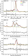Fig. A.1.

Same as Fig. 3, but for J0802+25. The spectra were smoothed using a boxcar of 4 to 6 pixels.

Fig. A.2.

Same as Fig. 3, but for J0945+17. The spectra were smoothed using a 5-pixel boxcar.

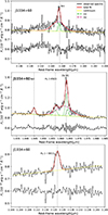Fig. A.3.

Same as Fig. 3, but for J1034+60. The spectra were smoothed using a boxcar of 4 to 5 pixels.

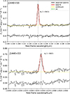Fig. A.4.

Same as Fig. 3 but for the H₂ lines detected in J1440+53. The spectra were smoothed using a 4-pixel boxcar.

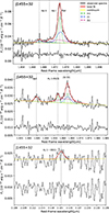Fig. A.5.

Same as Fig. 3, but for J1455+32. The spectra were smoothed using a boxcar of 4 to 7 pixels.

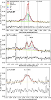Fig. A.6.

Same as Fig. 3, but for J1713+57. The spectra were smoothed using a boxcar of 4 to 5 pixels.

Table A.1.

Parameters derived from the fits of the lines of J0802+25.

Table A.2.

Parameters derived from the fits of the lines of J0945+17.

Table A.3.

Parameters derived from the fits of the lines of J1034+60.

Table A.4.

Parameters derived from the fits of the lines of J1440+53.

Table A.5.

Parameters derived from the fits of the lines of J1455+32.

Table A.6.

Parameters derived from the fits of the lines of J1713+57.

In the case of the two lower redshift QSO2s, J1034+60 and J1440+53, Brγ and [Si VI] were fit with two narrow components and a broad component. For J1440+53, an intermediate component was needed as well, and the Hβ fit was the reference for Brγ, Brγ for Brδ, [O III] for [Si VI], and H₂ 1−0S(1) for H₂ 1−0S(3). In the case of J1034+60, the reference fits were the same except for Brδ, whose reference was Hβ.

Appendix B: Electron density diagrams

Here we present the electron density and temperature diagnostics obtained for the QSO2s based on the [SII] method. As explained in Section 4.2.1, we used the [SII]λλ6716,6731Å doublet and [OIII]λ4363Å and [OIII]λ5007Å ratios to infer both n_e and T_e using Pyneb (Luridiana et al. 2015). The results found for the QSO2s are shown in Fig. B.1 and values are reported in Table 4.

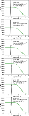Fig. B.1.

Diagnostic diagrams of the electron density and temperature computed from the [SII] and [OIII] ratios generated with Pyneb.

Appendix C: Outflow extent

Figs. C.1 to C.6 show the spectral regions and spatial profiles used to calculate the outflow extents. While in the case of the Paα and Brγ all the outflows are spatially resolved, in [Si VI] the outflows are not resolved for J0802+25, J1440+53, and J1455+32.

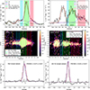Fig. C.1.

Spectral regions and spatial profiles used to calculate the outflow extent from Paα (left panels) and [Si VI] (right panels). Top row: Fits of the nuclear spectrum. The red and blue windows correspond to the wings of the lines, which are dominated by the outflows, while the green window captures the bulk of the narrow component. Middle row: Same spectral windows superimposed on the continuum-subtracted maps showing the line emission along the spectral and spatial directions. Bottom row: Average (i.e., weighted mean of the red and blue wings) continuum-subtracted spatial profiles of the Paα and [Si VI] outflows. The red solid line shows the Gaussian fit to the line profile, while the blue dashed lines corresponds to the seeing spatial profiles derived from observations of standard stars.

Fig. C.2.

Same as in Fig. C.1, but for J0945+17.

Fig. C.3.

Same as in Fig. C.1, but for J1034+60 and using Brγ instead of Paα.

Fig. C.4.

Same as in Fig. C.1, but for J1440+53 and using Brγ instead of Paα.

Fig. C.5.

Same as in Fig. C.1, but for J1455+32.

Fig. C.6.

Same as in Fig. C.1, but for J1713+57.

Appendix D: Outflow direct and physical properties

Table D.1.

Direct outflow properties of the QSO2s.

Table D.2.

Physical outflow properties obtained from the direct properties reported in Table D.1.

All Tables

Table 1.

Main properties of the QSO2s.

In the text

Table 2.

Summary of the GTC/EMIR long-slit observations.

In the text

Table 3.

Ranges of velocity shifts and FWHMs measured for the different components fit to the atomic lines.

In the text

Table 4.

Electron temperatures and densities obtained from the [SII] and TR methods.

In the text

Table 5.

Spatial extents of the outflow and narrow components measured from Paα/Brγ and [Si VI].

In the text

Table 6.

Comparison between the outflow properties of different samples of QSO2s.

In the text

Table 7.

List of QSO2s with NIR H₂ measurements reported in the literature.

In the text

Table A.1.

Parameters derived from the fits of the lines of J0802+25.

In the text

Table A.2.

Parameters derived from the fits of the lines of J0945+17.

In the text

Table A.3.

Parameters derived from the fits of the lines of J1034+60.

In the text

Table A.4.

Parameters derived from the fits of the lines of J1440+53.

In the text

Table A.5.

Parameters derived from the fits of the lines of J1455+32.

In the text

Table A.6.

Parameters derived from the fits of the lines of J1713+57.

In the text

Table D.1.

Direct outflow properties of the QSO2s.

In the text

Table D.2.

Physical outflow properties obtained from the direct properties reported in Table D.1.

In the text

All Figures

	Fig. 1. Sloan Digital Sky Survey gri images of the QSO2s. North is up and east to the left. Horizontal bars in the top-left corner of each image indicate the physical size of 5″. The images are 40″ × 40″ in size.
In the text

	Fig. A.1. Same as Fig. 3, but for J0802+25. The spectra were smoothed using a boxcar of 4 to 6 pixels.
In the text

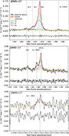	Fig. A.2. Same as Fig. 3, but for J0945+17. The spectra were smoothed using a 5-pixel boxcar.
In the text

	Fig. A.3. Same as Fig. 3, but for J1034+60. The spectra were smoothed using a boxcar of 4 to 5 pixels.
In the text

	Fig. A.4. Same as Fig. 3 but for the H₂ lines detected in J1440+53. The spectra were smoothed using a 4-pixel boxcar.
In the text

	Fig. A.5. Same as Fig. 3, but for J1455+32. The spectra were smoothed using a boxcar of 4 to 7 pixels.
In the text

	Fig. A.6. Same as Fig. 3, but for J1713+57. The spectra were smoothed using a boxcar of 4 to 5 pixels.
In the text

	Fig. B.1. Diagnostic diagrams of the electron density and temperature computed from the [SII] and [OIII] ratios generated with `Pyneb`.
In the text

Fig. C.1.

In the text

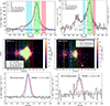	Fig. C.2. Same as in Fig. C.1, but for J0945+17.
In the text

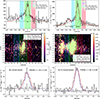	Fig. C.3. Same as in Fig. C.1, but for J1034+60 and using Brγ instead of Paα.
In the text

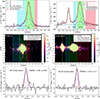	Fig. C.4. Same as in Fig. C.1, but for J1440+53 and using Brγ instead of Paα.
In the text

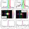	Fig. C.5. Same as in Fig. C.1, but for J1455+32.
In the text

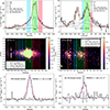	Fig. C.6. Same as in Fig. C.1, but for J1713+57.
In the text

Current usage metrics show cumulative count of Article Views (full-text article views including HTML views, PDF and ePub downloads, according to the available data) and Abstracts Views on Vision4Press platform.

Data correspond to usage on the plateform after 2015. The current usage metrics is available 48-96 hours after online publication and is updated daily on week days.

Initial download of the metrics may take a while.

[R1] Abazajian, K. N., Adelman-McCarthy, J. K., Agüeros, M. A., et al. 2009, ApJS, 182, 543 [Google Scholar]

[R2] Asplund, M., Amarsi, A. M., & Grevesse, N. 2021, A&A, 653, A141 [NASA ADS] [CrossRef] [EDP Sciences] [Google Scholar]

[R3] Astropy Collaboration (Price-Whelan, A. M., et al.) 2022, ApJ, 935, 167 [NASA ADS] [CrossRef] [Google Scholar]

[R4] Audibert, A., Ramos Almeida, C., García-Burillo, S., et al. 2023, A&A, 671, L12 [NASA ADS] [CrossRef] [EDP Sciences] [Google Scholar]

[R5] Audibert, A., Ramos Almeida, C., García-Burillo, S., et al. 2025, A&A, 699, A83 [NASA ADS] [CrossRef] [EDP Sciences] [Google Scholar]

[R6] Baron, D., & Netzer, H. 2019, MNRAS, 486, 4290 [Google Scholar]

[R7] Becker, R. H., White, R. L., & Helfand, D. J. 1995, ApJ, 450, 559 [Google Scholar]

[R8] Belli, S., Park, M., Davies, R. L., et al. 2024, Nature, 630, 54 [NASA ADS] [CrossRef] [Google Scholar]

[R9] Bertola, E., Cresci, G., Venturi, G., et al. 2025, A&A, 699, A220 [NASA ADS] [CrossRef] [EDP Sciences] [Google Scholar]

[R10] Bessiere, P. S., & Ramos Almeida, C. 2022, MNRAS, 512, L54 [NASA ADS] [CrossRef] [Google Scholar]

[R11] Bessiere, P. S., Ramos Almeida, C., Holden, L. R., Tadhunter, C. N., & Canalizo, G. 2024, A&A, 689, A271 [NASA ADS] [CrossRef] [EDP Sciences] [Google Scholar]

[R12] Bianchin, M., Riffel, R. A., Storchi-Bergmann, T., et al. 2022, MNRAS, 510, 639 [Google Scholar]

[R13] Bohn, T., Inami, H., Togi, A., et al. 2024, ApJ, 977, 36 [NASA ADS] [CrossRef] [Google Scholar]

[R14] Cardelli, J. A., Clayton, G. C., & Mathis, J. S. 1989, ApJ, 345, 245 [Google Scholar]

[R15] Carniani, S., Marconi, A., Maiolino, R., et al. 2015, A&A, 580, A102 [NASA ADS] [CrossRef] [EDP Sciences] [Google Scholar]

[R16] Cicone, C., Maiolino, R., Sturm, E., et al. 2014, A&A, 562, A21 [NASA ADS] [CrossRef] [EDP Sciences] [Google Scholar]

[R17] Cicone, C., Brusa, M., Ramos Almeida, C., et al. 2018, Nat. Astron., 2, 176 [Google Scholar]

[R18] Costa-Souza, J. H., Riffel, R. A., Souza-Oliveira, G. L., et al. 2024, ApJ, 974, 127 [Google Scholar]

[R19] Cresci, G., Mainieri, V., Brusa, M., et al. 2015a, ApJ, 799, 82 [Google Scholar]

[R20] Cresci, G., Marconi, A., Zibetti, S., et al. 2015b, A&A, 582, A63 [NASA ADS] [CrossRef] [EDP Sciences] [Google Scholar]

[R21] Dale, D. A., Sheth, K., Helou, G., Regan, M. W., & Hüttemeister, S. 2005, AJ, 129, 2197 [NASA ADS] [CrossRef] [Google Scholar]

[R22] Dall’Agnol de Oliveira, B., Storchi-Bergmann, T., Morganti, R., Riffel, R. A., & Ramakrishnan, V. 2023, MNRAS, 522, 3753 [CrossRef] [Google Scholar]

[R23] Dan, K. Y., Seebeck, J., Veilleux, S., et al. 2025, ApJ, 979, 68 [Google Scholar]

[R24] Davé, R., Anglés-Alcázar, D., Narayanan, D., et al. 2019, MNRAS, 486, 2827 [Google Scholar]

[R25] Davies, R., Baron, D., Shimizu, T., et al. 2020, MNRAS, 498, 4150 [Google Scholar]

[R26] Davies, R., Shimizu, T., Pereira-Santaella, M., et al. 2024, A&A, 689, A263 [NASA ADS] [CrossRef] [EDP Sciences] [Google Scholar]

[R27] Del Zanna, G., Dere, K. P., Young, P. R., & Landi, E. 2021, ApJ, 909, 38 [NASA ADS] [CrossRef] [Google Scholar]

[R28] Delaney, D., Berger, C., Hicks, E., et al. 2025, ApJ, 984, 163 [Google Scholar]

[R29] Dere, K. P., Landi, E., Mason, H. E., Monsignori Fossi, B. C., & Young, P. R. 1997, A&AS, 125, 149 [NASA ADS] [CrossRef] [EDP Sciences] [Google Scholar]

[R30] Di Matteo, T., Springel, V., & Hernquist, L. 2005, Nature, 433, 604 [NASA ADS] [CrossRef] [Google Scholar]

[R31] Doan, S., Satyapal, S., Reefe, M., et al. 2025, ApJS, 280, 57 [Google Scholar]

[R32] Emonts, B. H. C., Colina, L., Piqueras-López, J., et al. 2017, A&A, 607, A116 [NASA ADS] [CrossRef] [EDP Sciences] [Google Scholar]

[R33] Esparza-Arredondo, D., Ramos Almeida, C., Audibert, A., et al. 2025, A&A, 693, A174 [NASA ADS] [CrossRef] [EDP Sciences] [Google Scholar]

[R34] Ferland, G. J., Porter, R. L., van Hoof, P. A. M., et al. 2013, Rev. Mex. Astron. Astrofis., 49, 137 [Google Scholar]

[R35] Feruglio, C., Maiolino, R., Piconcelli, E., et al. 2010, A&A, 518, L155 [NASA ADS] [CrossRef] [EDP Sciences] [Google Scholar]

[R36] Fiore, F., Feruglio, C., Shankar, F., et al. 2017, A&A, 601, A143 [NASA ADS] [CrossRef] [EDP Sciences] [Google Scholar]

[R37] Fluetsch, A., Maiolino, R., Carniani, S., et al. 2019, MNRAS, 483, 4586 [NASA ADS] [Google Scholar]

[R38] Fluetsch, A., Maiolino, R., Carniani, S., et al. 2021, MNRAS, 505, 5753 [NASA ADS] [CrossRef] [Google Scholar]

[R39] Fonseca-Faria, M. A., Rodríguez-Ardila, A., Contini, M., Dahmer-Hahn, L. G., & Morganti, R. 2023, MNRAS, 524, 143 [CrossRef] [Google Scholar]

[R40] Gallagher, R., Maiolino, R., Belfiore, F., et al. 2019, MNRAS, 485, 3409 [NASA ADS] [CrossRef] [Google Scholar]

[R41] García-Bernete, I., Alonso-Herrero, A., García-Burillo, S., et al. 2021, A&A, 645, A21 [EDP Sciences] [Google Scholar]

[R42] Garzón, F., Abreu, D., Barrera, S., et al. 2006, in Ground-based and Airborne Instrumentation for Astronomy, eds. I. S. McLean, & M. Iye, (International Society for Optics and Photonics (SPIE)), 6269, 626918 [Google Scholar]

[R43] Garzón, F., Castro-Rodríguez, N., Insausti, M., et al. 2014, in Ground-based and Airborne Instrumentation for Astronomy V, eds. S. K. Ramsay, I. S. McLean, & H. Takami (International Society for Optics and Photonics (SPIE)), 9147, 91470U [Google Scholar]

[R44] Garzón, F., Balcells, M., Gallego, J., et al. 2022, A&A, 667, A107 [CrossRef] [EDP Sciences] [Google Scholar]

[R45] Girdhar, A., Harrison, C. M., Mainieri, V., et al. 2024, MNRAS, 527, 9322 [Google Scholar]

[R46] Harrison, C. M., & Ramos Almeida, C. 2024, Galaxies, 12, 17 [NASA ADS] [CrossRef] [Google Scholar]

[R47] Harrison, C. M., Alexander, D. M., Mullaney, J. R., & Swinbank, A. M. 2014, MNRAS, 441, 3306 [Google Scholar]

[R48] Harrison, C. M., Costa, T., Tadhunter, C. N., et al. 2018, Nat. Astron., 2, 198 [Google Scholar]

[R49] Hernandez, S., Smith, L. J., Jones, L. H., et al. 2025, ApJ, 983, 154 [Google Scholar]

[R50] Herrera-Camus, R., Janssen, A., Sturm, E., et al. 2020, A&A, 635, A47 [NASA ADS] [CrossRef] [EDP Sciences] [Google Scholar]

[R51] Hervella Seoane, K., Ramos Almeida, C., Acosta-Pulido, J. A., et al. 2023, A&A, 680, A71 [NASA ADS] [CrossRef] [EDP Sciences] [Google Scholar]

[R52] Hickox, R. C., Mullaney, J. R., Alexander, D. M., et al. 2014, ApJ, 782, 9 [NASA ADS] [CrossRef] [Google Scholar]

[R53] Holden, L. R., & Tadhunter, C. N. 2023, MNRAS, 524, 886 [NASA ADS] [CrossRef] [Google Scholar]

[R54] Holden, L. R., Tadhunter, C. N., Morganti, R., & Oosterloo, T. 2023, MNRAS, 520, 1848 [NASA ADS] [CrossRef] [Google Scholar]

[R55] Holden, L. R., Tadhunter, C., Audibert, A., et al. 2024, MNRAS, 530, 446 [NASA ADS] [CrossRef] [Google Scholar]

[R56] Holden, L. R., Smith, D. J. B., Arnaudova, M. I., et al. 2026, MNRAS, 545, staf2075 [Google Scholar]

[R57] Holt, J., Tadhunter, C. N., Morganti, R., & Emonts, B. H. C. 2011, MNRAS, 410, 1527 [NASA ADS] [Google Scholar]

[R58] Jones, A., Noll, S., Kausch, W., Szyszka, C., & Kimeswenger, S. 2013, A&A, 560, A91 [NASA ADS] [CrossRef] [EDP Sciences] [Google Scholar]

[R59] Kakkad, D., Mainieri, V., Vietri, G., et al. 2020, A&A, 642, A147 [NASA ADS] [CrossRef] [EDP Sciences] [Google Scholar]

[R60] Kakkad, D., Mainieri, V., Tanaka, T. S., et al. 2025, MNRAS, 541, 3534 [Google Scholar]

[R61] Kong, M., & Ho, L. C. 2018, ApJ, 859, 116 [NASA ADS] [CrossRef] [Google Scholar]

[R62] Lamastra, A., Bianchi, S., Matt, G., et al. 2009, A&A, 504, 73 [NASA ADS] [CrossRef] [EDP Sciences] [Google Scholar]

[R63] Lamperti, I., Pereira-Santaella, M., Perna, M., et al. 2022, A&A, 668, A45 [NASA ADS] [CrossRef] [EDP Sciences] [Google Scholar]

[R64] Luridiana, V., Morisset, C., & Shaw, R. A. 2015, A&A, 573, A42 [NASA ADS] [CrossRef] [EDP Sciences] [Google Scholar]

[R65] Maiolino, R., Russell, H. R., Fabian, A. C., et al. 2017, Nature, 544, 202 [Google Scholar]

[R66] Marconcini, C., Feltre, A., Lamperti, I., et al. 2025, A&A, 701, A113 [NASA ADS] [CrossRef] [EDP Sciences] [Google Scholar]

[R67] May, D., Rodríguez-Ardila, A., Prieto, M. A., et al. 2018, MNRAS, 481, L105 [NASA ADS] [CrossRef] [Google Scholar]

[R68] Mazzalay, X., Saglia, R. P., Erwin, P., et al. 2013, MNRAS, 428, 2389 [NASA ADS] [CrossRef] [Google Scholar]

[R69] McKaig, J. D., Satyapal, S., Laor, A., et al. 2024, ApJ, 976, 130 [Google Scholar]

[R70] Mercedes-Feliz, J., Anglés-Alcázar, D., Hayward, C. C., et al. 2023, MNRAS, 524, 3446 [NASA ADS] [CrossRef] [Google Scholar]

[R71] Moehler, S., Modigliani, A., Freudling, W., et al. 2014, A&A, 568, A9 [NASA ADS] [CrossRef] [EDP Sciences] [Google Scholar]

[R72] Mukherjee, D., Bicknell, G. V., Wagner, A. Y., Sutherland, R. S., & Silk, J. 2018, MNRAS, 479, 5544 [NASA ADS] [CrossRef] [Google Scholar]

[R73] Mullaney, J. R., Alexander, D. M., Fine, S., et al. 2013, MNRAS, 433, 622 [Google Scholar]

[R74] Müller-Sánchez, F., Prieto, M. A., Hicks, E. K. S., et al. 2011, ApJ, 739, 69 [Google Scholar]

[R75] Musiimenta, B., Speranza, G., Urrutia, T., et al. 2024, A&A, 687, A111 [NASA ADS] [CrossRef] [EDP Sciences] [Google Scholar]

[R76] Noll, S., Kausch, W., Barden, M., et al. 2012, A&A, 543, A92 [NASA ADS] [CrossRef] [EDP Sciences] [Google Scholar]

[R77] Oliva, E., & Moorwood, A. F. M. 1990, ApJ, 348, L5 [Google Scholar]

[R78] Osterbrock, D. E., & Ferland, G. J. 2006, Astrophysics of Gaseous Nebulae and Active Galactic Nnuclei (University Science Books) [Google Scholar]

[R79] Pereira-Santaella, M., Colina, L., García-Burillo, S., et al. 2018, A&A, 616, A171 [NASA ADS] [CrossRef] [EDP Sciences] [Google Scholar]

[R80] Perna, M., Arribas, S., Ji, X., et al. 2025, A&A, 694, A170 [NASA ADS] [CrossRef] [EDP Sciences] [Google Scholar]

[R81] Pierce, J. C. S., Tadhunter, C., Ramos Almeida, C., et al. 2023, MNRAS, 522, 1736 [NASA ADS] [CrossRef] [Google Scholar]

[R82] Ramos Almeida, C., & Ricci, C. 2017, Nat. Astron., 1, 679 [Google Scholar]

[R83] Ramos Almeida, C., Pérez García, A. M., Acosta-Pulido, J. A., et al. 2006, ApJ, 645, 148 [Google Scholar]

[R84] Ramos Almeida, C., Piqueras López, J., Villar-Martín, M., & Bessiere, P. S. 2017, MNRAS, 470, 964 [NASA ADS] [CrossRef] [Google Scholar]

[R85] Ramos Almeida, C., Acosta-Pulido, J. A., Tadhunter, C. N., et al. 2019, MNRAS, 487, L18 [NASA ADS] [CrossRef] [Google Scholar]

[R86] Ramos Almeida, C., Bischetti, M., García-Burillo, S., et al. 2022, A&A, 658, A155 [NASA ADS] [CrossRef] [EDP Sciences] [Google Scholar]

[R87] Ramos Almeida, C., García-Bernete, I., Pereira-Santaella, M., et al. 2025, A&A, 698, A194 [NASA ADS] [CrossRef] [EDP Sciences] [Google Scholar]

[R88] Ramos Almeida, C., Asensio Ramos, A., Westerdorp Plaza, C., et al. 2026, A&A, 706, A100 [NASA ADS] [CrossRef] [EDP Sciences] [Google Scholar]

[R89] Reyes, R., Zakamska, N. L., Strauss, M. A., et al. 2008, AJ, 136, 2373 [Google Scholar]

[R90] Riffel, R. A., Storchi-Bergmann, T., Riffel, R., et al. 2023, MNRAS, 521, 1832 [NASA ADS] [CrossRef] [Google Scholar]

[R91] Riffel, R. A., Souza-Oliveira, G. L., Costa-Souza, J. H., et al. 2025, ApJ, 982, 69 [Google Scholar]

[R92] Rodríguez-Ardila, A., & Cerqueira-Campos, F. 2025, Front. Astron. Space Sci., 12, 1548632 [Google Scholar]

[R93] Rodríguez-Ardila, A., Prieto, M. A., Mazzalay, X., et al. 2017, MNRAS, 470, 2845 [Google Scholar]

[R94] Rose, M., Tadhunter, C., Ramos Almeida, C., et al. 2018, MNRAS, 474, 128 [Google Scholar]

[R95] Rupke, D. S. N., & Veilleux, S. 2013, ApJ, 775, L15 [NASA ADS] [CrossRef] [Google Scholar]

[R96] Rupke, D. S. N., Gültekin, K., & Veilleux, S. 2017, ApJ, 850, 40 [NASA ADS] [CrossRef] [Google Scholar]

[R97] Santoro, F., Oonk, J. B. R., Morganti, R., Oosterloo, T. A., & Tadhunter, C. 2016, A&A, 590, A37 [NASA ADS] [CrossRef] [EDP Sciences] [Google Scholar]

[R98] Schawinski, K., Koss, M., Berney, S., & Sartori, L. F. 2015, MNRAS, 451, 2517 [Google Scholar]

[R99] Speranza, G., Ramos Almeida, C., Acosta-Pulido, J. A., et al. 2022, A&A, 665, A55 [NASA ADS] [CrossRef] [EDP Sciences] [Google Scholar]

[R100] Speranza, G., Ramos Almeida, C., Acosta-Pulido, J. A., et al. 2024, A&A, 681, A63 [NASA ADS] [CrossRef] [EDP Sciences] [Google Scholar]

[R101] Su, K.-Y., Hopkins, P. F., Hayward, C. C., et al. 2019, MNRAS, 487, 4393 [NASA ADS] [CrossRef] [Google Scholar]

[R102] Tadhunter, C., Morganti, R., Rose, M., Oonk, J. B. R., & Oosterloo, T. 2014, Nature, 511, 440 [Google Scholar]

[R103] Tody, D. 1986, SPIE Conf. Ser., 627, 733 [Google Scholar]

[R104] Tody, D. 1993, ASP Conf. Ser., 52, 173 [NASA ADS] [Google Scholar]

[R105] Trindade Falcão, A., Kraemer, S. B., Crenshaw, D. M., et al. 2022, MNRAS, 511, 1420 [Google Scholar]

[R106] Vayner, A., Zakamska, N., Wright, S. A., et al. 2021, ApJ, 923, 59 [CrossRef] [Google Scholar]

[R107] Villar-Martín, M., Arribas, S., Emonts, B., et al. 2016, MNRAS, 460, 130 [Google Scholar]

[R108] Villar Martín, M., Castro-Rodríguez, N., Pereira Santaella, M., et al. 2023, A&A, 673, A25 [NASA ADS] [CrossRef] [EDP Sciences] [Google Scholar]

[R109] Woo, J.-H., Bae, H.-J., Son, D., & Karouzos, M. 2016, ApJ, 817, 108 [Google Scholar]

[R110] York, D. G., Adelman, J., Anderson, J. E., Jr., et al. 2000, AJ, 120, 1579 [NASA ADS] [CrossRef] [Google Scholar]

[R111] Zakamska, N. L., & Greene, J. E. 2014, MNRAS, 442, 784 [Google Scholar]

[R112] Zanchettin, M. V., Feruglio, C., Bischetti, M., et al. 2021, A&A, 655, A25 [NASA ADS] [CrossRef] [EDP Sciences] [Google Scholar]

[R113] Zanchettin, M. V., Feruglio, C., Massardi, M., et al. 2023, A&A, 679, A88 [NASA ADS] [CrossRef] [EDP Sciences] [Google Scholar]

[R114] Zanchettin, M. V., Ramos Almeida, C., Audibert, A., et al. 2025, A&A, 695, A185 [NASA ADS] [CrossRef] [EDP Sciences] [Google Scholar]

[R115] Zinger, E., Pillepich, A., Nelson, D., et al. 2020, MNRAS, 499, 768 [CrossRef] [Google Scholar]

[R116] Zubovas, K., & Maskeliūnas, G. 2023, MNRAS, 524, 4819 [CrossRef] [Google Scholar]