| Issue |
A&A
Volume 708, April 2026
|
|
|---|---|---|
| Article Number | A151 | |
| Number of page(s) | 17 | |
| Section | The Sun and the Heliosphere | |
| DOI | https://doi.org/10.1051/0004-6361/202557814 | |
| Published online | 03 April 2026 | |
The Sun as an X-ray star
V. A new method to retrieve coronal filling factors
1
Institut für Astronomie & Astrophysik, Eberhard Karls Universität Tübingen, Sand 1, 72076 Tübingen, Germany
2
INAF – Osservatorio Astronomico di Palermo, Piazza del Parlamento 1, 90134 Palermo, Italy
★ Corresponding author: This email address is being protected from spambots. You need JavaScript enabled to view it.
Received:
24
October
2025
Accepted:
5
March
2026
Abstract
Context. Stellar coronae are unresolved in X-rays, so inferences about their structure rely on spectral analysis. The Sun-as-an-X-ray-star (SaXS) approach uses the Sun as a spatially resolved template to interpret stellar spectra, but previous SaXS implementations were indirect and computationally heavy.
Aims. We present a new SaXS implementation that converts solar emission measure distributions (EMDs) of distinct coronal region types into XSPEC spectral components, and we aim to test whether broadband X-ray spectra alone can recover the lling factors of those region types.
Methods. We built XSPEC multi-temperature spectral models for four solar region types (background or quiet coronae, active regions, cores, and flares) by considering EMDs derived from the analysis of Yohkoh/SXT data and by translating each EMD bin to an isothermal VAPEC component, or, alternatively, to a nonequilibrium–ionization collisional plasma VNEI component. These XSPEC models were fit (using PyXspec) to two one-hour DAXSS spectra representative of quiescent (29 June, 2022) and flaring (25 Apr., 2022) states. Best-fit normalizations were converted into projected areas and filling factors and compared with near-coincident Hinode/XRT full-disk images for validation.
Results. Using the Yohkoh/SXT EMDs, we found that the spectrum of the quiescent Sun is dominated by active-region emission (filling factor ≈21%), with the background corona poorly constrained, while the spectrum of the flaring Sun is best described by a combination of active regions, cores, and flares with filling factors ≈14%, ≈3%, and ≈0.07%, respectively. We checked that the dominant components qualitatively match spatial features in Hinode/XRT images. Major limitations are the DAXSS low-energy calibration cutoff (∼0.7 keV) and the small, nonuniform Yohkoh EMD sample adopted, which may affect constraints on cool, low-emission regions and on elemental line emission.
Conclusions. We demonstrate that our SaXS implementation enables direct retrieval of coronal filling factors from broadband X-ray spectra and provides a physically motivated alternative to ad hoc few-temperature fits. This approach can therefore potentially be routinely applied to stellar X-ray spectra to infer the distribution of coronal structures.
Key words: techniques: spectroscopic / Sun: activity / Sun: corona / Sun: X-rays / gamma rays / stars: activity / stars: coronae
© The Authors 2026
 Open Access article, published by EDP Sciences, under the terms of the Creative Commons Attribution License (https://creativecommons.org/licenses/by/4.0), which permits unrestricted use, distribution, and reproduction in any medium, provided the original work is properly cited.
This article is published in open access under the Subscribe to Open model. This email address is being protected from spambots. You need JavaScript enabled to view it. to support open access publication.
1. Introduction
High-energy observations are crucial for understanding solar and stellar coronae, where plasma is magnetically confined and heated to millions of kelvin (Pallavicini et al. 1981). The solar corona hosts a variety of magnetic structures that appear bright and hot in X-rays (Reale 2014). These structures play a central role in shaping solar activity and in addressing the long-standing coronal heating problem (Klimchuk 2006, 2015). In contrast, for stars other than the Sun, X-ray emission remains spatially unresolved: stellar coronae appear as point sources whose spectra represent the integrated contribution of regions spanning a wide range of temperatures and densities. Interpreting such spectra therefore relies on indirect approaches that link the observed emission to the underlying physical structures on the stellar surface. The Sun provides a unique opportunity to bridge this gap. As the only star whose corona can be spatially resolved, it can serve as a reference for stellar coronal studies through Sun-as-a-star methods that attempt to decipher how the Sun would appear observationally if it were a distant star (e.g., Peres et al. 2000; Livingston et al. 2007; Collier Cameron et al. 2019). Using detailed solar observations enabled by the proximity of the Sun, we can infer the goings-on on the surface and in the atmosphere of distant stars of other late-type, magnetically active stars. While the activity levels of stars span at least three orders of magnitude (e.g., Caramazza et al. 2023) that arise from different interior structures (determining the dynamo) and different evolutionary stages (determining the rotation rate), the Sun is the only spatially resolvable template we have. Methods that enable a direct comparison of solar and stellar data can uncover the extent to which the coronae of other stars resemble that of the Sun and what differences (if any) exist.
One such approach is to construct scaling relations for parameters that are observable from the X-ray spectra of stars (namely the total emission measure and the temperature) from models of heating and energy transport that are based on observations of the Sun. In such models, the corona is characterized by the length of quiescent or flaring loops and their filling factor (see, e.g., Rosner et al. 1978; Shibata & Yokoyama 2002; Takasao et al. 2020). While such descriptions enable a straightforward comparison of the average conditions in the coronae of stars in different activity states, they provide very limited information on the actual spatial structure of the stellar corona. This can be achieved through the Sun-as-an-X-ray-star (SaXS) method, which we investigated in this study; it quantifies the coronal magnetic structure of late-type stars through X-ray spectroscopy, making use of an assumed solar-stellar analogy.
The SaXS method (Orlando et al. 2000; Peres et al. 2000; Reale et al. 2001) was motivated by the observation that the Sun consists of various types of magnetically active regions whose brightness, temperature, and density increase in the following order: (i) background corona (BKC), representing the quiet corona; (ii) active regions (ARs), consisting of magnetic loops that trap plasma at temperatures of a few megakelvin; (iii) cores of active regions (COs), composed of hot, dense magnetic loops; and (iv) flares (FL), which are explosive energy releases occurring in coronal loops resulting from magnetic reconnection. These coronal region types were originally demarcated only by their pixel intensities, in units of DN/s, on images obtained with the Soft X-ray Telescope (SXT; Tsuneta et al. 1991) on board the Yohkoh satellite (Ogawara et al. 1991). The abundance of the different types of these coronal regions is a marker of solar activity, and their variations are used to study the solar cycle (e.g., Peres et al. 2000; Orlando et al. 2001).
The different types of magnetically active structures on the Sun have distinct X-ray emission measure distributions (EMDs). These distributions, as observed by Yohkoh/SXT, were presented by Orlando et al. (2001, 2004) for the BKC, AR, and CO regions, and by Reale et al. (2001) for individual flares of the following GOES classes: C5.8, M1.0, M1.1, M2.8, M4.2, M7.6, X1.5, and X9.0.
In the first applications of the SaXS method, these Yohkoh EMDs were used to predict the occurrence and amount of the different solar coronal region types on HD 81809 (Favata et al. 2008; Orlando et al. 2017), ϵ Eri (Coffaro et al. 2020), and Kepler 63 (Coffaro et al. 2022). This was achieved by an approach that involved creating synthetic total emission measures, EMtot, by scaling the EMDs of the individual coronal region types, EMDreg, by their filling factors, ffreg, and summing them: EMtot = ∑regffregEMDreg. The filling factors represent the percentage of the stellar corona covered by different types of magnetic region. For each total emission measure distribution, defined by the filling factors of the various magnetic region types, an X-ray spectrum was synthesized. These synthetic spectra were then analyzed as if they were observational data, that is, fit in XSPEC with thermal models to derive the coronal properties, namely, the X-ray temperature (Tx) and luminosity (Lx). By comparing the synthetic (Tx, Lx) pairs with the corresponding values obtained from the same thermal model to the observed stellar X-ray spectrum, we identified the combination of filling factors that best reproduces the observation. This allowed us to infer the relative contributions and importance of the different coronal regions in the target star.
In its first application to the solar-like star HD 81809, Favata et al. (2008) synthesized a corona composed of solar ARs and COs, which Orlando et al. (2004) had shown to characterize the solar corona throughout its activity cycle. The study found that the X-ray temperature and luminosity predicted from the AR and CO filling factors characteristic of the solar cycle bracketed the observed values (Tx, Lx) of HD 81809. A subsequent study of the same star, based on an approximately doubled XMM-Newton monitoring time, revealed a wider scatter of the star in the (Tx, Lx) plane (Orlando et al. 2017). Consequently, Orlando et al. (2017), along with later studies on other stars (Coffaro et al. 2020, 2022), computed a full grid of synthetic spectra–based on a corresponding grid of filling factors–and compared the resulting best-fit parameters with the observed stellar properties.
For ϵ Eri, this approach revealed a high (60–90%) surface coverage with magnetic regions throughout the whole activity cycle (Coffaro et al. 2020). This finding was considered as a potential origin of the saturation phenomenon (Fleming et al. 1989). In this interpretation, increasing the stellar spin rate beyond a certain threshold does not increase the star’s X-ray luminosity because the corona is already fully covered with magnetic structures and cannot accommodate additional emitting regions.
These earlier applications of the SaXS method to stellar X-ray spectra thus demonstrate its high scientific value for quantifying the solar–stellar connection paradigm. However, although the method provided reasonable estimates of the filling factors and far-reaching results on the structure of stellar coronae, the previous implementation of the SaXS method, it is complex, indirect, and computationally demanding.
We present a new, more efficient implementation of the SaXS technique. It consists in converting the EMDs of solar coronal regions derived from Yohkoh images into empirical X-ray spectral models that can be directly used to fit stellar X-ray spectra. The aim to retrieve the filling factors of the corona of a given star with each of these solar coronal region types was achieved by weighting the contribution of the model of each coronal region type in the fitting and finding the best combination of them. However, before applying this technique to distant unresolved stars, it had to be calibrated on solar spectra. This requires solar X-ray spectra covering the continuous range of energies (0.2–10 keV) observed with astrophysical facilities such as the X-ray Multi-Mirror Mission (XMM-Newton; Jansen et al. 2001) or the extended ROentgen Survey with an Imaging Telescope Array (eROSITA; Predehl et al. 2021) on board the Russian Spektrum-Roentgen–Gamma mission (SRG; Sunyaev et al. 2021), which perform X-ray spectroscopy of other stars. Such solar broadband, soft X-ray spectra were lacking until recently.
Beginning in 2016, the Miniature X-ray Solar Spectrometer CubeSat-1 (MinXSS-1; Mason et al. 2016), its successor MinXSS-2 (Mason et al. 2020), and a sounding rocket flight of the Dual-zone Aperture X-ray Solar Spectrometer (DAXSS; Woods et al. 2017, 2023) provided the first solar spectra in the 0.5–10 keV band. More recently, DAXSS is being operated on board the INSPIRESat-1 satellite (Chandran et al. 2021), delivering continuous observations suitable for testing our method.
In this paper, we present a new implementation of the SaXS method and apply it to solar X-ray spectra from DAXSS/INSPIRESat-1, covering two different levels of solar activity. We verified the consistency between spectrally derived coronal regions and their filling factors using near-simultaneous, full-disk Hinode/XRT images. In Sect. 2, we describe the construction of XSPEC spectral models from EMDs of different coronal region types and the retrieval of filling factors from spectral fits. In Sect. 3, we present their application to DAXSS data. In Sect. 4, we discuss the results, and finally, in Sect. 5, we provide our conclusions.
2. Definition of XSPEC models for the SaXS method
In this section, we describe how we obtain coronal region spectral models from the solar emission measure distributions observed with Yohkoh/SXT. Specifically, we converted the emission measure distribution of each solar coronal region EM(T)reg observed with Yohkoh into a corresponding empirical spectral model, which we then implemented in PyXSPEC (Gordon & Arnaud 2021).
The EMDs per unit projected area derived from Yohkoh/SXT data by Orlando et al. (2001), Orlando et al. (2004), and Reale et al. (2001) for the coronal structures described in Sect. 1 are shown in Fig. 1. These EMDs were derived from a limited set of Yohkoh/SXT observations, namely 23 synoptic images containing various region types (Orlando et al. 2001), 78 observations following a single active region through its evolution (Orlando et al. 2004), and eight flares covering different phases of their evolution from rise to peak and decay (Reale et al. 2001). To facilitate the development of the SaXS methodology and to avoid complications from temporal variations, in this work we used time-averaged EMDs for all coronal-region types.
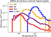 |
Fig. 1. EMDs of BKC, AR, CO, and FL-AVG regions as described in Sect. 1. The y-axis shows the emission measure per unit area, in units of 1044 cm−5. All EMDs shown here represent time-averaged distributions constructed from multiple snapshots of flares or other types of regions. |
The time-averaged EMDs of the individual flares (C5.8, M1.0, M1.1, M2.8, M4.2, M7.6, X1.5, and X9.0) are shown in Fig. 2. For simplicity, we combined the EMDs of all the flares into a single representative “average flare” EMD (hereafter FL-AVG). When constructing FL-AVG, we accounted for the fact that flares with different peak amplitudes (which define their GOES class) occur at different frequencies. Accordingly, FL-AVG was obtained as a weighted average of the individual flare EMDs, where the weights were determined by the slope of the cumulative flare-energy frequency distribution (FFD) in logarithmic space, α, following N(E)∝Eα. Here, E denotes the flare energy, and we adopted α = −1.54, which is the FFD slope derived for solar X-ray flares from Yohkoh observations (Aschwanden & Parnell 2002). The energy of the eight individual flares was estimated using the empirical relation between the GOES peak flux, FGOES1, and the corresponding white-light flare (WLF)2 energy, EWLF from Namekata et al. (2017). This relation is expressed as log(EWLF) = a + b ⋅ log(FGOES), with coefficients a = 33.67 and b = 0.87. The resulting average FL-AVG EMD is shown in blue in Figs. 1 and 2.
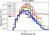 |
Fig. 2. EMDs of C5.8, M1.0, M1.1, M2.8, M4.2, M7.6, and X1.5 flares as presented by Reale et al. (2001) (individual colors) along with their weighted average EMD (FL-AVG, blue). The y-axis shows the emission measure per unit area, in units of 1044 cm−5. |
To derive a spectral model from each of the EMDs, we assume that each bin i in the EMD of a given type of coronal region (Ti, reg, EMi, reg) represents emission from an isothermal plasma. The total EMD of that type of region is then described by a distinct distribution of several isothermal plasmas effectively constituting a multi-temperature plasma. Such a multi-temperature plasma model can be constructed in XSPEC (Arnaud et al. 1999) as a sum of i isothermal models for a plasma in collisional-ionization equilibrium (APEC; Smith et al. 2001) or a plasma that is out of the equilibrium state (NEI; Bradshaw et al. 2004). Both models also have variants which allow to adjust the abundances of individual chemical elements (VAPEC or VNEI). Each individual component of these models is characterized by (Ti, reg, Normi, reg), as well as the coronal abundances as input parameters. For the nonequilibrium model an additional parameter is the ionization timescale, τion.
We implemented this modeling approach using PyXspec (Gordon & Arnaud 2021), a Python package that provides an interface to XSPEC. The abundances are here defined for the star, i.e., they are assumed to be the same throughout the whole corona, regardless of the type of magnetic structure. Therefore, each coronal-region model, Mreg, is defined as
 (1)
(1)
or as
 (2)
(2)
where Mreg can be MBKC, MAR, MCO, or MFL − AVG and the XSPEC models can be substituted by their variable-abundance versions. In this work, we adopted the Feldman Standard Extended Coronal abundances code (FELD in XSPEC; Feldman 1992). The spectral models for all four region types and their individual components are visualized in Appendix A.1 for the example of the APEC model, and they assume an abundance of 1.0.
In Eqs. (1) and (2), the normalizations, Normi, reg, are fixed values obtained from the EMi, reg values of the region type’s EMD using the relation
 (3)
(3)
where D is the distance to the star in centimeters. As mentioned above, the elemental abundances can either be set as a global value, expressed in units of solar abundances using the APEC or the NEI model, or customized for each chemical element individually using the VAPEC or VNEI variants. In principle, the latter variable-abundance models are more appropriate when the elemental abundances are already known for different temperatures on the Sun, or when applying the models to stars whose coronal abundances are expected to differ from the solar values.
Solar and stellar broadband soft X-ray spectra can then be fit with a spectral model, Mspec, that is an additive combination of the spectral models for various types of regions. Hereby, the contribution from a given region, Mreg, as a whole can be scaled up or down during spectral fitting, with the scaling measured as the total normalization of the coronal region, Normreg. The spectral model to be fit is thus
 (4)
(4)
The total emission measure of a particular type of region on the star, EMreg, tot, is just the total emission measure per unit area of that type of region on the Sun, EMreg, ⊙,
 (5)
(5)
scaled by Normreg obtained from the spectral fit
 (6)
(6)
On the Sun, Normreg is simply the projected area of that coronal region in cm2. Therefore, the filling factor of the region on the Sun, ffreg, is
 (7)
(7)
where Aproj, ⊙ is the projected area of the solar disk. When observing a star in X-rays, the detected emission originates not only from the visible photospheric disk, but also from the extended corona above the limb. This is also true for the broadband solar X-ray spectra from DAXSS. To account for this, we included the vertical extension of the corona in the total projected area, Aproj, ⊙. We achieved this by approximating the extent of the solar corona by its scale height, which is defined as
 (8)
(8)
where μ = 0.6 is the mean molecular weight of the fully ionized coronal plasma, and TBKC is the emission-measure–weighted average temperature of the background corona. The corresponding effective projected area is thus given as
 (9)
(9)
where R⊙ is the solar radius. This formulation includes both the photospheric disk and the coronal layer extending approximately one scale height beyond the solar limb. This amounts to a total area of Aproj, ⊙ ≈ 1.7 × 1022 cm2.
3. Application of SaXS to solar data
The new version of the SaXS method, which consists of defining XSPEC spectral models for the different coronal region types and fitting them to observed spectra, is introduced here for the first time. Therefore, before proceeding to applying this approach to stellar X-ray spectra, we provide the first test on the Sun itself. The goal is analogous to that of future applications to other stars, for example our first application to AD Leo (Joseph et al., in prep.), that is, to retrieve the coronal filling factors for the different types of magnetic structures. In contrast to other stars, however, the Sun offers the possibility to verify the results on actual images, namely to check whether the filling factors derived from the spectra are consistent with the structures seen at the same time in full-disk observations of the Sun. To this end, we applied the new SaXS methodology to soft X-ray spectra from DAXSS, obtained the best fitting combination of coronal-region models (Sect. 3.3), and derived their corresponding filling factors. Subsequently, we validated the results of the spectral fits on solar Hinode/XRT images taken close in time (Sect. 3.4).
3.1. DAXSS observations and selection of representative spectra
We obtained DAXSS Level 2 data stored as mission-length NCDF files on the DAXSS mission website3. DAXSS data are updated periodically as the mission continues to downlink new observations daily. At the time of writing, version 2.1.0 was available, covering February 28, 2022 to October 24, 2023. This time span corresponds to the middle of the rise phase of Solar Cycle No. 25.
The DAXSS data can be unpacked to provide light curves and spectra in the 0.4–12.0 keV band. DAXSS spectra are available in native cadence (a few minutes), one-hour, and one-day averages. We used the one-hour-averaged spectra as our ultimate goal, with the SaXS method used to test whether solar-type regions are found on stars by fitting spectral models to stellar spectra; these are typically averaged over several hour timescales to collect sufficient photon statistics for reliable spectral fits.
To test the performance of the SaXS models for different solar-activity states, we used the DAXSS/INSPIRESat-1 mission light curve to identify the two observations with the lowest count rate and highest count rate. These correspond to June 29, 2022 at 12:44 and April 25, 2022 at 02:18, respectively, and we extracted their corresponding spectra. We refer to these hereafter as the quiescent-Sun and flaring-Sun observations, respectively. The GOES light curves acquired simultaneously with the DAXSS observations reveal the Sun’s activity level, which is clearly different for the two observations (see Fig. 3). The April 25 observation corresponds to an M class flare (in the 1–8 Å band used for GOES flare classification), while the June 29 observation shows minimal activity with only a small B class flare barely rising above the surrounding quiescent background level.
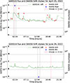 |
Fig. 3. GOES X-ray flux in 1–8 Å band (green) and DAXSS count rates for April 25, 2022 and June 29, 2022. Horizontal gray lines demarcate the GOES flare classes A, B, C, M, and X. The epochs of the DAXSS spectra selected for analysis in this paper are marked in the DAXSS light curve as blue crosses, and vertical dashed lines indicate the one-hour exposure time of the spectra. The Hinode/XRT synoptic images used to verify the SaXS method correspond to the time period indicated by the vertical pink band. |
3.2. Refining EMDs based on spectral fitting results
We applied the SaXS XSPEC models (Sect. 2) separately to the two DAXSS spectra described in Sect. 3.1, starting with the simplest type of plasma model, which is APEC. During the fitting, the elemental abundances were fixed to quiescent solar values, adopting the Feldman Standard Extended Coronal abundances (feld in XSPEC; Feldman 1992) code, with the XSPEC parameter for the abundance set to unity. Upper limits were imposed corresponding to a total filling factor of 100% to ensure that the derived projected areas did not exceed the solar corona’s total projected area defined in Sect. 2. The primary quantities obtained from each fit are the filling factors, ffreg (Eq. (7)), for all region types included in the best-fit model.
Initial fits using spectral models derived from all EMDs reveal systematic discrepancies with the observed spectral shape. Specifically, the observed spectra exhibit steeper high-energy drop-offs than predicted by any of the SaXS models in the 0.7–3.0 keV range. This is illustrated in Fig. 4, in which we overlay (without fitting) the different SaXS spectral models to the two observed DAXSS spectra.
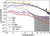 |
Fig. 4. DAXSS spectra corresponding to the lowest and highest count rates in the DAXSS light curve along with arbitrarily scaled SaXS models of the various types of coronal regions. This demonstrates the steeper slope of the solar spectra compared with the spectrum of all types of coronal region which indicates an over-contribution of low-signal EM bins (see text in Sect. 3.2). |
We attribute these discrepancies to the bins at the EMD tails, in particular the high-temperature tails of CO, AR, and BKC, which have low values of emission measure (see Fig. 1) but seem to over-contribute to the spectral models.
We therefore redefined the EMD for each type of region, restricting it to bins within one order of magnitude of the peak of the EMD, as shown in Appendix C.1. The need for such an empirically motivated adjustment indicates that the EMDs used here are not fully representative of the region types. This is most likely related to the time evolution of the magnetic structures and their associated EMDs. We discuss this further in Sect. 4.3.
We regenerated all SaXS spectral models in Eqs. (1) and (2) from the restricted EMDs. In Appendix D.1, we show how the APEC variants of the spectral models for the different types of coronal region change as a result of our modification of the EMDs. Clearly, the EMD bins that have since been removed (translucent bins in Appendix. C.1) drastically increase the flux in the high-energy portion of the spectra, making them inconsistent with the observed DAXSS spectra.
3.3. Spectral fits and results
Using the restricted EMDs, we systematically tested the individual components on the two DAXSS spectra introduced in Sect. 3.1 as explained in the following. For both spectra, we started the fitting with the APEC model. Subsequently, we used the more complicated model VAPEC and, for the flare spectrum, the nonequilibrium ionization model VNEI.
3.3.1. Quiescent-Sun spectrum
Starting with the APEC version of the SaXS models by considering any single type of region, the AR model provides the best fit to the quiescent-Sun spectrum with a filling factor of 23.54 ± 0.31% (Fig. 5, top panel). Residuals, especially at low energies, suggest the need for an additional lower temperature component. Adding the BKC model (Fig. 5, bottom panel) improves the spectral fit ( versus 5.78 previously). However, the emission from the much brighter AR dominates, and the BKC contributes only minimally to the overall spectrum. This results in its filling factor being poorly constrained and the AR filling factor changing only marginally. This two-region model has the filling factors ffBKC = 94.12 ± 65.85% and ffAR = 21.83 ± 0.4%. Despite the improvement, strong residuals remain, particularly from spectral line features.
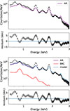 |
Fig. 5. DAXSS spectrum from 29 June, 2022 representing the quiescent Sun fit with APEC-based SaXS models. The model consisting of the AR component alone is shown on the top figure and with the added BKC component is shown on the bottom figure. |
To investigate whether these residuals could be attributed to incorrect values for the elemental abundances, we varied the abundances of Ar, Ca, Fe, Mg, Si, and S following the recommendations of Woods et al. (2023), which provide guidelines for modeling DAXSS spectra based on thecoronal temperature regime. For the BKC model (analogous to their quiet-Sun < 4 MK category), we only varied Mg and Si, while the other elements were kept fixed at the standard value of 1.0 with respect to the Feldman (1992) coronal standard. For AR and CO models (analogous to the AR at 4–8 MK), we varied all six elements. To reduce the number of free parameters, we tied Mg and Si abundances across all region types, and we tied Ar, Ca, Fe, and S across the AR and CO models. We allowed a conservative 20% variation by constraining all abundances to lie between 0.8 and 1.2, reflecting the expectation that the Feldman coronal abundances should be approximately correct, with only small deviations possible. The abundance values derived from this fit with the VAPEC model are listed in Table B.1 (Appendix B).
Incorporating variable abundances improved the fit to  (Fig. 6), with filling factors ffBKC = 45.20 ± 149.53% and ffAR = 21.31 ± 5.76%. However, most elements reach the imposed limits (Mg, Si, and Fe at 1.2; S at 0.8), while Ar and Ca remain poorly constrained with large uncertainties. This behavior, combined with the still elevated χred2 value, suggests that abundances differ by more than 20% from the FELD values or that the underlying atomic data require updating (see discussion in Sect. 4.3).
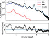 |
Fig. 6. DAXSS spectrum from 29 June, 2022 representing the quiescent Sun fit with BKC and AR models with variable abundances (VAPEC). |
3.3.2. Flaring-Sun spectrum
We applied the same methodology to the flare spectrum. Given the enhanced high-energy emission compared with the quiescent-Sun spectrum (see Fig. 4), we began the fitting with the APEC models using FL-AVG, which, among all individual region types, produces the best fit to the high-energy part of the spectrum. This model fits the high-energy portion well, but significant low-energy residuals remain, yielding  (Fig. 7, top panel).
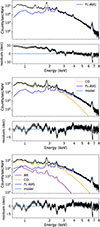 |
Fig. 7. DAXSS spectrum from 25 Apr. 2022, representing the Flaring Sun with FL-AVG alone (top), FL-AVG + CO (middle), and FL-AVG + CO + AR (bottom), all using APEC-based SAXS models. |
After adding CO, the model also successfully fits the low-energy spectrum with strongly reduced residuals,  (Fig. 7 middle panel), and filling factors, ffCO = 4.47 ± 0.069% and ffFL − AVG = 0.06 ± 0.00068%. Since cores typically accompany ARs, we included the AR model, which provides a further marginal improvement (
 ) but leaves the AR filling factor poorly constrained at ffAR = 47.51 ± 13.97%. Except for its softest part, the spectrum is dominated by core and flare emission, with filling factors of ffCO = 4.07 ± 0.14% and ffFL − AVG = 0.062 ± 0.00077% in the three-component fit (Fig. 7, bottom panel). Adding a BKC component did not further improve the fit (
 ) because the emission is dominated by the other regions with higher emission per unit area. The BKC component is very poorly constrained, yielding ffBKC = (5.4 ± 1102)×10−3%.
To further improve the fit of the flare spectrum, we employed variable abundances, as in the quiescent-Sun case, for all region types. We used the VAPEC version of the spectral models for the AR and CO and the VNEI version for FL-AVG. For the FL-AVG model (analogous to the Woods et al. (2023) “Flare” category at > 6 MK), we also varied all six elements with abundances tied to the AR and CO values. The resulting fit shows substantial improvement, with  (Fig. 8) and filling factors of ffAR = 14.72 ± 23.67%, ffCO = 3.37 ± 0.22%, and ffFL = 0.07 ± 0.0014%.
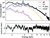 |
Fig. 8. DAXSS spectrum from 25 Apr., 2022 representing the flaring Sun fit with AR, CO, and FL-AVG models with variable abundances (VAPEC) for AR and CO and nonequilibrium ionization (VNEI) for FL-AVG. |
This fit decreases the high-energy residuals seen in the APEC best fit that overestimated line emission, especially the Fe line complex at ≈6.7 keV. Its strength is now reduced despite the Fe abundance being increased to its upper limit (Z = 1.2 Z⊙, feld). This is due to the nonequilibrium effect of suppressing higher temperature lines. The derived ionization timescale is τion = (2.29 ± 0.21)×1011 s cm−3. This is below the value of ∼1012 s cm−3 at which most ions approach ionization equilibrium in flare-heating models (Lee et al. 2019); it is therefore consistent with the partial nonequilibrium ionization expected during impulsive heating episodes (Bradshaw et al. 2004).
3.3.3. Summary of best-fit spectral models
To summarize, our best-fit spectral model for the quiescent Sun is based on VAPEC, and it comprises an AR and a BKC. For the flaring Sun, our best-fit spectral model comprises FL-AVG, CO, and BKC, and it is based on VNEI for FL-AVG and on VAPEC for the other two region types. The filling factors derived for these best-fit models are summarized in Table 1.
Coronal-region filling factors from SaXS and image-based solar catalogs.
3.4. Validation with Hinode observations
To verify if the filling factors inferred from the spectral analysis are consistent with the structures seen in contemporaneous images of the Sun, we obtained the Hinode/XRT Level 2 synoptic composite images from the Hinode archive (4; Takeda et al. 2016) taken closest in time to the DAXSS observations (Fig. 9 and Appendix E.1, which shows enhanced fainter features in the flaring-Sun observation). These are the images from April 25, 2022 at 02:06 and June 29, 2022 at 18:03 (vertical pink bands in Fig. 3). The April 25 image was taken with the Be_thin filter and does not require any corrections for light leaks; it is therefore appropriate for use in this work as it is. On the other hand, for the June 29 observation taken with the Al_mesh filter, we only needed to apply a light-leak correction. We did this using the XRTpy function “remove_lightleak” in Python (XRTpy (v0.5.0)5; Velasquez et al. 2024) for Hinode X-Ray Telescope data analysis.
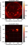 |
Fig. 9. Hinode/XRT images corresponding to quiescent- and flaring-Sun DAXSS observations (top and bottom panels, respectively). |
Since the different types of coronal regions are defined based on Yohkoh/SXT pixel intensities (IBKC < IAR < ICO < IFL), we can identify corresponding regions in Hinode/XRT images by progressively masking pixels based on the filling factors derived from the spectra. To better capture the total coronal output as observed in the integrated DAXSS spectra–which, as unresolved stellar observations, include emission extending above the limb–we also included pixels extending to one solar scale height (see Eq. (8)) above the limb. For this test, we used the filling factors derived from our best-fit SaXS models: the variable-abundance VAPEC-based models for the quiescent-Sun observation and VAPEC-based models in combination with the VNEI-based FL-AVG component for the flaring-Sun observation. We masked the brightest pixels corresponding to each region type’s filling factor, starting with the hottest and brightest component and working downward in temperature. For example, using the best-fit model filling factors of the flaring-Sun spectrum from Table 1, we designated the brightest 0.07% of pixels as belonging to flares. Next, we excluded these and designated the brightest 3.37% of the remaining pixels as belonging to cores, and further excluding these, we assigned the next brightest 14.72% of pixels to ARs. We proceeded analogously for the quiescent-Sun spectrum.
Figures 10 and 11 visualize the areas on the Sun identified this way for the quiescent- and the flaring-Sun observation, respectively. Appendix F.1 shows a zoomed-in view of the flaring region. The different regions detected with the SaXS method are marked in Figs. 10 and 11 with different colorbars. The rest of the solar corona (white in Figs. 10 and 11) is covered by the fainter types of structures (e.g., BKC for the case of the flare spectrum), which do not contribute significantly to the spectrum and, therefore, are not part of the best-fit model.
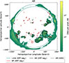 |
Fig. 10. Hinode/XRT image during quiescent-Sun observation with highlighted pixels showing the AR component (green gradient) (Sect. 3.4) identified from spectral fitting in Sect. 3.3.1. The solar-limb boundaries, shown by the green circles, are taken from the Hinode/XRT segmentation maps. The inner boundary defines the reference area used in the filling-factor calculations. The black and red contours correspond to active regions and bright points, respectively, as identified in the Hinode/XRT segmentation database (Adithya et al. 2021). The active regions simultaneously detected by various solar instruments and registered in the HEK (Hurlburt et al. 2012) are shown as black bounding boxes. |
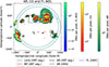 |
Fig. 11. Hinode/XRT image taken during the flaring-Sun observation, showing pixels color-coded by coronal regions (Sect. 3.4) whose filling factors were determined from spectral fitting in Sect. 3.3.2: AR (green gradient), CO (orange gradient), and FL-AVG (blue–teal gradient). The solar limb boundaries (Limb (XRT seg.)), shown by the green circles, are taken from the Hinode/XRT segmentation maps. The inner boundary defines the reference area used in the filling factor calculations. The black and red contours correspond to active regions (AR (XRT seg.)) and bright points (BP (XRT seg.)), respectively, as identified in the Hinode/XRT segmentation database (Adithya et al. 2021). The flares (FL (HEK)) and active regions (AR (HEK)) simultaneously detected by various solar instruments and registered in the HEK (Hurlburt et al. 2012) are shown as black and blue bounding boxes, respectively. |
To validate our image decomposition, we compared the regions identified through the SaXS-derived filling factors with independent solar-feature catalogs. Specifically, we used bounding boxes from the public Heliophysics Event Knowledgebase (HEK) (Hurlburt et al. 2012) for active regions and flares (which HEK labels as AR and FL, respectively)–shown as black and blue boxes in Figs. 10 and 11–and segmentation maps from the Hinode/XRT segmentation database6 (Adithya et al. 2021) for ARs and bright points (labeled as AR and BP in the database), shown as colored contours in Figs. 10 and 11. The Hinode/XRT segmentation database also provides inner and outer solar limb boundaries. As the features stored in both databases are restricted to within the inner solar limb, we adopted the inner boundary to define the reference area for the calculation of filling factors from their region definitions. While these catalogs use the same acronyms as our SaXS region types, their definitions differ: catalog features are identified morphologically in images, while our spectral components are defined by their characteristic thermal structure.
The filling factors we derived from the information given in the databases are summarized together with those from our SaXS spectral analysis in Table 1. For the flaring-Sun observation (25 Apr., 2022), the HEK bounding boxes yield an AR filling factor almost three times higher than that obtained from the XRT database segmentation. This discrepancy primarily arises from the different instruments and region-identification methods employed in the two datasets. A smaller contribution to the difference may come from a temporal mismatch: the XRT segmentation by Adithya et al. (2021) corresponds to 05:48 UT, about three hours after the synoptic Hinode/XRT composite at 02:06 UT, by which time the flare had already subsided (see the GOES light curve in Fig. 3). This time offset explains the slight spatial displacement between the XRT segmentation contours and the regions visible in the Hinode/XRT image.
For the quiescent-Sun observation (29 June, 2022), the HEK bounding boxes again give higher AR filling factors than the Hinode/XRT segmentation maps. In this case, temporal effects are negligible, since the Sun was in a quiet phase and no major activity changes occurred between the observations. The discrepancy instead reflects the use of different instruments and different classification techniques in the two datasets. Absolute agreement between the approaches is therefore not expected, owing to these intrinsic methodological and instrumental differences.
Comparing the information from the HEK bounding boxes and XRT image segmentations to our image decomposition based on the SaXS spectral modeling shows that the same dominant coronal structures (active regions and flaring sites) are consistently identified across all approaches. However, our SaXS spectral filling factors are systematically significantly higher than those derived from the data bases. This is because HEK data and XRT segmentations are restricted to features within the solar limb. In contrast, our SaXS-derived maps include emission extending up to one solar scale height above the limb, to better capture the total coronal output that would be observed from an unresolved stellar perspective. The additional emission we capture with SaXS analysis on full-disk spectra can be identified in Figs. 10 and 11 as the colored areas outside the inner circle that denotes the solar limb. It is easily seen that a high fraction of AR emission comes from beyond the limb. We discuss these results further in Sect. 4.2.
4. Discussion
4.1. The new SaXS method: A physical description of spectra and dynamics in stellar coronae
We developed a fundamentally new approach to the SaXS prescription for comparing stellar X-ray observations to solar data. Our new implementation consists of creating X-ray spectral models for the individual types of solar coronal regions. Specifically we define XSPEC models for BKC, AR, CO, and FL-AVG, by converting their Yohkoh/SXT EMDs each into a multi-temperature spectral model in which each temperature-component of the EMD is appropriately weighted. These XSPEC models can replace previous uninformed spectral fitting yielding a physical description of the emitting plasma in the corona of magnetically active stars. We demonstrate this here in the example of the Sun itself.
Previously, quiescent and flaring solar spectra from DAXSS were analyzed using one- or two-temperature isothermal models with fixed or variable abundances (e.g., Schwab et al. 2020, 2023). These models provide a reasonable approximation of the integrated emission from different coronal regions that cannot be directly resolved on other stars, and they are standard practice in stellar X-ray spectroscopy. Schwab et al. (2020) found that the hotter temperature component in their two-temperature fits was associated with ARs visible in contemporaneous solar images. Their quiescent Sun fits yielded χred2 ∼ 7.7, with a 1T model and ∼4.5 with 2T components, further improving to ∼3.9 when allowing elemental abundances to vary in the fit. These results are comparable to χred2 values of 4.68 and 1.16, which we obtained for our SaXS model fits on the quiescent- and flaring-Sun spectra, respectively. This shows that the current version of SaXS spectral models achieve fits of similar quality to standard multi-temperature models while additionally providing a physical link between spectral components and specific types of coronal structures. Specifically, it enables direct retrieval of coronal filling factors. Further improvements of the SaXS models are foreseen in the future, as we discuss in Sect. 4.3
4.2. Consistency check of the new SaXS approach on solar data
In the first application of the new SaXS method, we tested the technique on the Sun itself. We selected two DAXSS spectra, one representing the quiescent and one the flaring Sun. We found that the quiescent-Sun spectrum was best fit with the BKC and AR models (Fig. 5, bottom panel), and the flaring-Sun spectrum was best fit with AR, CO, and FL-AVG regions (Fig. 7, bottom panel). The filling factors derived from the SaXS spectral fitting were then visualized on Hinode/XRT images as described in Sect. 3.4. To validate our results, we compared the regions identified through our SaXS spectral analysis on the Hinode/XRT images with image segmentations carried out by others.
Overall, we found good spatial correspondence between the regions detected by our method and those listed in the HEK and the Hinode/XRT databases, although the filling factors do not match exactly. There are several reasons for this. First, both HEK and Hinode/XRT segmentations are strictly limited to features within the solar limb, whereas we also included emission from within one solar scale height above the limb. The location of the solar limb itself was adopted from the Hinode/XRT segmentation maps and used as the reference area in our filling-factor calculations. Our choice reflects the stellar-analogy goal of our study – i.e., to account for all coronal emission that would be observed if the Sun were seen as an unresolved star. Second, HEK regions are identified using a variety of instruments and wavelengths, each with its own detection and validation procedures, while the Hinode/XRT maps are based solely on broadband X-ray data. Our approach, in contrast, relies primarily on intensity thresholds applied uniformly to broadband images. Finally, some categories used in our analysis (e.g., CO regions) are not explicitly listed in current solar-feature databases, further limiting one-to-one correspondence. Despite these differences, the same major coronal structures were consistently detected by all methods, indicating that the filling factors inferred from SaXS are physically meaningful.
4.3. Open issues
Despite the compelling qualitative and quantitative results presented above, several limitations of the present implementation of the SaXS method must be acknowledged and will be addressed in future work.
First, we are currently restricted to applying our spectral models with a low-energy cutoff of 0.7 keV because DAXSS is not well calibrated below this threshold (Schwab et al. 2020, 2023). This means that the energy range of 0.2–0.7 keV, which constitutes an important part of the spectra provided by stellar X-ray observatories such as XMM-Newton and eROSITA, remains untested in the present analysis. This soft-energy regime is essential for constraining the spectral contribution of low-temperature coronal structures such as BKCs and ARs. In fact, in our tests on the DAXSS spectra the filling factors of the components contributing the highest emission to the spectra can be constrained well (see Sect. 3.2), but those contributing little to the emission can be constrained only poorly, even if they occupy the largest projected area on the corona.
For example, in the quiescent-Sun spectrum, the fit improved only slightly when the BKC component was added, whereas in the flaring-Sun spectrum the inclusion of BKC worsened the fit. This does not imply that these regions were absent from the solar disk at the time of observation; rather, their emission measure per unit area is too low for their contribution to be detectable in the integrated spectrum with its limitation to E > 0.7 keV. Consequently, our method currently provides reasonable constraints for the higher temperature and more emissive coronal structures, but is intrinsically less sensitive to low-emission and low-temperature regions. We stress that this limitation is specific to the DAXSS-based validation presented here and does not apply to future applications of the SaXS framework to stellar X-ray spectra, for which the reliable soft X-ray coverage of instruments such as XMM-Newton and eROSITA will provide much stronger constraints on cooler coronal components.
In order to obtain a reasonably good fit to the DAXSS spectra, meaning that systematic trends in residuals over a large energy range are avoided, we had to modify the original Yohkoh EMDs. The restriction of the EMDs, illustrated in Appendix. C.1 and described in Sect. 3.2, is purely based on the observation that both the quiescent-Sun and flaring-Sun spectra have steeper high-energy drop-offs than any of the spectral models that were created using the entire original EMD set, as illustrated in Fig. 4.
This behavior highlights an intrinsic property of the EMD library currently adopted. The Yohkoh/SXT EMDs are based on a limited and nonuniform sample of observations and should therefore be regarded as a set of time-averaged templates for different classes of coronal structures rather than as exhaustive descriptions of their full variability. As a result, they are not necessarily representative of the instantaneous coronal configuration sampled by the DAXSS observations. The discrepancy also likely arises because the EMDs used in this paper represent averages over multiple individual EMDs, whereas the DAXSS data reflect a specific realization of coronal structures at a given time. Orlando et al. (2004) showed that the high-temperature tails of AR and CO EMDs depend strongly on evolutionary stage and activity level: newly emerged ARs and COs exhibit pronounced hot tails, while more evolved or less active structures display much weaker high-temperature emission. The need to suppress the high-temperature tails in order to fit the DAXSS spectra therefore suggests that the coronal structures present during the observations were predominantly evolved and characterized by relatively low levels of activity.
The restriction of the EMDs applied here should thus not be interpreted as an ad hoc tuning introduced to force agreement with the data, but rather as a controlled sensitivity test that highlights the strong leverage of small amounts of hot plasma on the integrated spectral slope. Importantly, this restriction does not alter the characteristic temperatures or the relative ordering of the coronal region types. The resulting filling factors remain physically plausible and are independently supported by their qualitative spatial correspondence with Hinode/XRT images. A larger set of EMDreg sampling different evolutionary stages and activity levels of individual region types is needed to obtain more precise and fully robust results from the SaXS spectral fit.
With the empirically “restricted EMDs”, the overall slope of both the quiescent- and flaring-Sun spectra can be described with suitable combinations of BKC, AR, CO, and FL-AVG. However, the χred2 remains high, and systematic residuals are present that appear to be associated to individual emission lines and line complexes (e.g., Woods et al. 2023; Telikicherla et al. 2024). The residuals improve only marginally when allowing for variable abundances in the fitting process. Schwab et al. (2020), which included a spectral analysis on DAXSS data using conventional two-temperature VAPEC models, also found significant residuals and concluded that updated atomic calculations might be necessary. The authors explicitly pointed out the 0.8 keV region, which has the strongest residuals in our quiescent-Sun spectrum fit. In this spectral region, Fe XVII and Fe XVIII lines dominate. Their formation temperatures (∼3 − 6 MK) are present in our SaXS EMDs. Therefore, these residuals possibly reflect limitations in the atomic data underlying the spectral models as the feld atomic database used in XSPEC dates back to 1992 (Feldman 1992).
Finally, we note that we did not explicitly model the contribution from coronal holes (CHs). While CHs are prominent in X-ray images during solar minimum, their emission is characterized by low temperatures (T ≤ 1.5 MK) and low emission measures. Consequently, their spectral signature is concentrated below 0.7 keV, making them undetectable in the current DAXSS validation. While CH emission may be important for stars at the lowest activity levels (e.g., Caramazza et al. 2023), it is expected to be negligible compared to AR, CO, and FL components in the active stars that are the primary focus of the SaXS technique.
4.4. Outlook regarding application of the new SaXS approach to stellar X-ray spectra
The primary goal of the SaXS framework is to place the Sun in a stellar context by decomposing the solar corona into its fundamental physical constituents (BKC, AR, CO, and FL) and testing whether stellar X-ray spectra can be reconstructed from different combinations of these building blocks. This approach evaluates the “scaled-up Sun” paradigm: a successful reconstruction implies that the stellar corona operates under similar physical processes as the Sun, albeit within different magnetic-flux and energy regimes.
The Sun’s total X-ray EMD varies significantly over the Solar Cycle (e.g., Fig. 4 of Orlando et al. 2001). Stellar EMDs within this range can therefore be explained in terms of different solar coronal region types. However, faster rotation and stronger dynamo action in younger stars systematically shift their EMDs to higher temperatures and emission measures compared to older, less active stars, including the Sun (Güdel 2004). Consequently, more active stars are expected to have higher filling factors of brighter, hotter solar-like magnetic structures. This was confirmed in previous SaXS applications (Orlando et al. 2017; Coffaro et al. 2020), where CO and FL structures dominated the emission, albeit covering only a few percent of the corona.
Systematic deviations from this solar-based reconstruction signal genuine physical differences in stellar environments. For instance, very active stars or observations dominated by large flares may feature magnetic structures unlike those on the Sun. Caution is therefore required in the interpretation of derived filling factors for situations in which the solar templates appear inadequate, and the inability to fit such X-ray spectra marks the limits of the solar–stellar connection.
In addition, applying SaXS to other stars requires accounting for several other known differences. First, coronal abundances of stars are known to be different from those of the Sun (Testa 2010). Therefore, in applications of SaXS to other stars the VAPEC model should be used with the abundance values as free fit parameters. Alternatively, elemental abundances can be independently determined from high-resolution spectra prior to SaXS modeling. This would minimize the number of free parameters and reduce fitting complexity. A second important difference between the Sun and other magnetically active stars concerns coronal densities. For other stars, the normalizations, Normreg, obtained from SaXS spectral fits do not translate directly into projected surface areas for the region types as they do for the Sun (see Sect. 2). Instead, Normreg can be used to derive the total emission measure (Eq. (6)), from which, together with measured electron densities and the typical size of the coronal region types’ filling factors can be calculated. Electron densities can be measured from density-sensitive line ratios in high-resolution stellar X-ray spectra (e.g., Ness et al. 2004), and these measurements reveal densities that are systematically higher than solar values. Therefore, electron densities should ideally be measured from high-resolution spectra of the target star for a range of coronal temperature regimes.
In the forthcoming study by Joseph et al. (in prep.), we present a first application of the new SaXS implementation to an XMM-Newton observation of the flare star AD Leo. This observation comprises the Great Flare of Nov 2021, a superflare with a GOES class of X1400 (Stelzer et al. 2022) providing a benchmark to test the regime of validity for the solar–stellar connection under extreme conditions.
5. Conclusions
We developed and tested a new implementation of the SaXS method that converts observed solar coronal region EMDs into spectral models to be used within XSPEC. They can therefore be used to fit stellar and solar X-ray spectra providing, as main output, the filling factors of the different types of magnetic structures in the corona.
In this work, we focused on validating the new SaXS approach on the Sun. Applied to DAXSS observations of the quiescent and the flaring Sun, the SaXS spectral models qualitatively reproduce the spectra reasonably well. Their predicted filling factors were validated against Hinode/XRT X-ray images. Our results show that the filling factors of dominant emitting regions in the solar corona (e.g., ARs during quiescence and AR+CO+FL-AVG during flares) can be constrained robustly, while weaker emission regions remain less well constrained. Significant line residuals persist even with variable abundance modeling, with most elemental abundances reaching their imposed limits, suggesting that the underlying atomic data in the Feldman coronal abundance library may require updating. Obtaining simultaneous constraints on both abundances and filling factors is, therefore, challenging. Ideally, coronal abundances should be independently constrained before being applied within the SaXS framework.
This work presents the first implementation of SaXS with separate spectral models for each type of coronal region, tested directly against solar spectra. The SaXS spectral models thus provide a practical bridge between solar observations and unresolved stellar coronae, offering an alternative to traditional fitting of a model consisting of a few temperatures. While empirical, the approach is grounded in the similarity of stellar and solar EMDs, and it allows direct retrieval of coronal region filling factors for spatially unresolved surfaces of active stars. Thus, it opens a path toward quantifying stellar activity in terms of the relative abundances of distinct coronal structures, rather than relying on purely phenomenological global plasma temperatures.
We validated our spectrally derived filling factors against the HEK and Hinode/XRT databases of independently classified solar regions. These datasets provide a valuable cross-check, although their spatial definitions and temporal coverage differ substantially. The HEK entries were derived from multiple instruments and wavelengths, while the Hinode/XRT segmentations are based solely on broadband X-ray data. The inclusion of the emission from the limb together with differences in the definition of the boundaries between the different region types explains the larger filling factor we obtained with SaXS compared to the results in the two databases.
The limitations of the present work include the low-energy response cutoff of DAXSS at 0.7 keV and the reliance on a small set of Yohkoh-derived EMDs that do not systematically sample all solar magnetic region types. Nevertheless, the method provides a framework that can be refined and tested with larger solar samples (making use of contemporaneous Hinode, DAXSS, and GOES data). Already, in its present version, its application to stars provides interesting insight (Joseph et al., in prep.). – In summary, this work introduces spectral SaXS as a viable tool for studying magnetically active stars, enabling direct inference of coronal region filling factors from X-ray spectra and providing a new approach to characterizing stellar activity and testing the solar–stellar connection.
Acknowledgments
WMJ acknowledges support by the Bundesministerium für Wirtschaft und Energie through the Deutsches Zentrum für Luft- und Raumfahrt e.V. (DLR) under grant numbers FKZ 50 OR 2208. DAXSS (INSPIRESat-1) solar soft X-ray spectral irradiance data is provided by LASP/University of Colorado (MinXSS/DAXSS team); we used version 2.1.0 of the Level 2 data product. Hinode is a Japanese mission developed and launched by ISAS/JAXA, collaborating with NAOJ as a domestic partner, NASA and STFC (UK) as international partners. Scientific operation of the Hinode mission is conducted by the Hinode science team organized at ISAS/JAXA. This team mainly consists of scientists from institutes in the partner countries. Support for the post-launch operation is provided by JAXA and NAOJ (Japan), STFC (U.K.), NASA, ESA, and NSC (Norway).
References
- Adithya, H. N., Kariyappa, R., Shinsuke, I., et al. 2021, Sol. Phys., 296, 71 [Google Scholar]
- Arnaud, K., Dorman, B., & Gordon, C. 1999, Astrophysics Source Code Library [record ascl:9910.005] [Google Scholar]
- Aschwanden, M. J., & Parnell, C. E. 2002, ApJ, 572, 1048 [NASA ADS] [CrossRef] [Google Scholar]
- Bradshaw, S. J., Del Zanna, G., & Mason, H. E. 2004, A&A, 425, 287 [NASA ADS] [CrossRef] [EDP Sciences] [Google Scholar]
- Caramazza, M., Stelzer, B., Magaudda, E., et al. 2023, A&A, 676, A14 [NASA ADS] [CrossRef] [EDP Sciences] [Google Scholar]
- Chandran, A., Fang, T.-W., Chang, L., et al. 2021, Adv. Space Res., 68, 2616 [Google Scholar]
- Coffaro, M., Stelzer, B., Orlando, S., et al. 2020, A&A, 636, A49 [EDP Sciences] [Google Scholar]
- Coffaro, M., Stelzer, B., & Orlando, S. 2022, A&A, 661, A79 [NASA ADS] [CrossRef] [EDP Sciences] [Google Scholar]
- Collier Cameron, A., Mortier, A., Phillips, D., et al. 2019, MNRAS, 487, 1082 [Google Scholar]
- Favata, F., Micela, G., Orlando, S., et al. 2008, A&A, 490, 1121 [NASA ADS] [CrossRef] [EDP Sciences] [Google Scholar]
- Feldman, U. 1992, Phys. Scr., 46, 202 [CrossRef] [Google Scholar]
- Fleming, T. A., Gioia, I. M., & Maccacaro, T. 1989, ApJ, 340, 1011 [Google Scholar]
- Gordon, C., & Arnaud, K. 2021, Astrophysics Source Code Library [record ascl:2101.014] [Google Scholar]
- Güdel, M. 2004, A&ARv, 12, 71 [CrossRef] [Google Scholar]
- Hurlburt, N., Cheung, M., Schrijver, C., et al. 2012, Sol. Phys., 275, 67 [Google Scholar]
- Jansen, F., Lumb, D., Altieri, B., et al. 2001, A&A, 365, L1 [NASA ADS] [CrossRef] [EDP Sciences] [Google Scholar]
- Klimchuk, J. A. 2006, Sol. Phys., 234, 41 [Google Scholar]
- Klimchuk, J. A. 2015, Philos. Trans. R. Soc. Lond. Ser. A, 373, 20140256 [NASA ADS] [Google Scholar]
- Lee, J.-Y., Raymond, J. C., Reeves, K. K., et al. 2019, ApJ, 879, 111 [Google Scholar]
- Livingston, W., Wallace, L., White, O. R., & Giampapa, M. S. 2007, ApJ, 657, 1137 [CrossRef] [Google Scholar]
- Mason, J. P., Woods, T. N., Caspi, A., et al. 2016, J. Spacecr. Rockets, 53, 328 [NASA ADS] [CrossRef] [Google Scholar]
- Mason, J. P., Woods, T. N., Chamberlin, P. C., et al. 2020, Adv. Space Res., 66, 3 [Google Scholar]
- Namekata, K., Sakaue, T., Watanabe, K., et al. 2017, ApJ, 851, 91 [Google Scholar]
- Neidig, D. F. 1989, Sol. Phys., 121, 261 [NASA ADS] [CrossRef] [Google Scholar]
- Ness, J. U., Güdel, M., Schmitt, J. H. M. M., Audard, M., & Telleschi, A. 2004, A&A, 427, 667 [NASA ADS] [CrossRef] [EDP Sciences] [Google Scholar]
- Ogawara, Y., Takano, T., Kato, T., et al. 1991, Sol. Phys., 136, 1 [NASA ADS] [CrossRef] [Google Scholar]
- Orlando, S., Peres, G., & Reale, F. 2000, ApJ, 528, 524 [NASA ADS] [CrossRef] [Google Scholar]
- Orlando, S., Peres, G., & Reale, F. 2001, ApJ, 560, 499 [NASA ADS] [CrossRef] [Google Scholar]
- Orlando, S., Peres, G., & Reale, F. 2004, A&A, 424, 677 [NASA ADS] [CrossRef] [EDP Sciences] [Google Scholar]
- Orlando, S., Favata, F., Micela, G., et al. 2017, A&A, 605, A19 [NASA ADS] [CrossRef] [EDP Sciences] [Google Scholar]
- Pallavicini, R., Golub, L., Rosner, R., et al. 1981, ApJ, 248, 279 [NASA ADS] [CrossRef] [Google Scholar]
- Peres, G., Orlando, S., Reale, F., Rosner, R., & Hudson, H. 2000, ApJ, 528, 537 [NASA ADS] [CrossRef] [Google Scholar]
- Predehl, P., Andritschke, R., Arefiev, V., et al. 2021, A&A, 647, A1 [EDP Sciences] [Google Scholar]
- Reale, F. 2014, Liv. Rev. Sol. Phys., 11, 4 [Google Scholar]
- Reale, F., Peres, G., & Orlando, S. 2001, ApJ, 557, 906 [CrossRef] [Google Scholar]
- Rosner, R., Tucker, W. H., & Vaiana, G. S. 1978, ApJ, 220, 643 [Google Scholar]
- Schwab, B. D., Sewell, R. H. A., Woods, T. N., et al. 2020, ApJ, 904, 20 [Google Scholar]
- Schwab, B. D., Woods, T. N., & Mason, J. P. 2023, ApJ, 945, 31 [Google Scholar]
- Shibata, K., & Yokoyama, T. 2002, ApJ, 577, 422 [CrossRef] [Google Scholar]
- Smith, R. K., Brickhouse, N. S., Liedahl, D. A., & Raymond, J. C. 2001, ApJ, 556, L91 [Google Scholar]
- Song, Y. L., Tian, H., Zhang, M., & Ding, M. D. 2018, A&A, 613, A69 [NASA ADS] [CrossRef] [EDP Sciences] [Google Scholar]
- Stelzer, B., Caramazza, M., Raetz, S., Argiroffi, C., & Coffaro, M. 2022, A&A, 667, L9 [NASA ADS] [CrossRef] [EDP Sciences] [Google Scholar]
- Sunyaev, R., Arefiev, V., Babyshkin, V., et al. 2021, A&A, 656, A132 [NASA ADS] [CrossRef] [EDP Sciences] [Google Scholar]
- Švestka, Z. 1970, Sol. Phys., 13, 471 [Google Scholar]
- Takasao, S., Mitsuishi, I., Shimura, T., et al. 2020, ApJ, 901, 70 [NASA ADS] [CrossRef] [Google Scholar]
- Takeda, A., Yoshimura, K., & Saar, S. H. 2016, Sol. Phys., 291, 317 [Google Scholar]
- Telikicherla, A., Woods, T. N., & Schwab, B. D. 2024, ApJ, 966, 198 [CrossRef] [Google Scholar]
- Testa, P. 2010, Space Sci. Rev., 157, 37 [NASA ADS] [CrossRef] [Google Scholar]
- Tsuneta, S., Acton, L., Bruner, M., et al. 1991, Sol. Phys., 136, 37 [Google Scholar]
- Velasquez, J., Murphy, N., Reeves, K., et al. 2024, J. Open Source Softw., 9, 6396 [Google Scholar]
- Woods, T. N., Caspi, A., Chamberlin, P. C., et al. 2017, ApJ, 835, 122 [Google Scholar]
- Woods, T. N., Schwab, B., Sewell, R., et al. 2023, ApJ, 956, 94 [Google Scholar]
These fluxes, by definition, determine the GOES class of the flares.
White-light flares are characterized by a sudden enhancement of optical continuum emission (Švestka 1970; Neidig 1989; Song et al. 2018).
Appendix A: SaXS spectral models and their components
Figure A.1 illustrates the SaXS spectral models implemented in XSPEC. They were constructed from the emission measure distributions (EMDs) of the different coronal region types defined in Sect. 2. Each panel shows the composite model spectrum (colored line) together with the individual APEC components (grey curves) that represent the isothermal plasma contributions corresponding to the temperature bins of the respective EMD. The colors denote the coronal region type: red for the background corona (BKC), purple for active regions (AR), yellow for cores (CO), and blue for the averaged flare distribution (FL-AVG). These models form the basis of the SaXS fitting procedure described in Sect. 3, where they are combined in varying proportions to reproduce observed solar soft X-ray spectra.
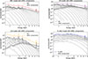 |
Fig. A.1. Composite SaXS spectral models made with XSPEC (colored) and their individual APEC components (grey) for the main solar coronal region types used in the SaXS method (see Sect. 2). Colors indicate the coronal region type: red for the background corona (BKC), purple for the active regions (AR), yellow for the cores (CO), and blue for the averaged flares (FL-AVG). |
Appendix B: Derived elemental abundances
Table B.1 lists the elemental abundances derived from spectral fits with variable abundances to the Quiescent Sun (2022 June 29) and Flaring Sun (2022 April 25) observations. Following Woods et al. (2023), we varied specific elements appropriate to the dominant coronal region types. Abundances refer to the Feldman standard extended coronal abundances (Feldman 1992).
Elemental abundances for quiescent and flaring solar conditions measured with respect to the Feldman (1992) coronal standard.
Appendix C: Restricted vs original EMDs
Figure C.1 compares the original Yohkoh EMDs of the coronal region types introduced in Sect. 1 with their restricted versions used in this work (Sect. 3.2). The restricted EMDs include only temperature bins within one order of magnitude of the peak emission measure of each distribution, effectively removing the low- and high-temperature tails that were found to overestimate the flux in the high-energy portion of the observed solar broad-band spectra. In Fig. C.1 opaque lines correspond to the restricted EMDs adopted for the spectral modeling, while the transparent lines show those parts of the original Yohkoh/SXT EMDs that we have discarded. The orignal EMDs are, thus, a combination of the opaque and translucent bins. They are also presented in Fig. 1.
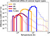 |
Fig. C.1. Emission measure distributions of the BKC, AR, CO and FL-AVG regions as described in Sect. 1. The opaque lines are the restricted distributions we use in this paper (described in Sect. 3.2), and the transparent lines show those parts of the original Yohkoh/SXT EMDs that we have discarded. The original EMDs are thus the combination of the opaque and transparent bins, and are also shown in Fig. 1. |
Appendix D: Comparison of SaXS spectral models from restricted vs original EMDs
Figure D.1 compares the SaXS spectral models in XSPECobtained from the full emission measure distributions (EMDs) with those generated from the restricted EMDs introduced in Sect. 3.2. Each panel shows the model corresponding to one coronal region type: background corona (BKC, red), active regions (AR, purple), cores (CO, yellow), and averaged flares (FL-AVG, blue). Solid lines represent the spectral models derived from the original full EMDs, while dashed lines show the models constructed from the reduced EMDs that exclude low- and high-temperature bins with emission measures more than one order of magnitude below the EMD peak. These comparisons illustrate how removing the low-signal EMD tails reduces excess high-energy flux, leading to improved agreement with the observed DAXSS spectra.
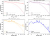 |
Fig. D.1. Comparison between composite SaXS spectral models in XSPEC derived from the full (solid lines) and restricted (dashed lines) emission measure distributions for the main coronal region types defined in Sect. 3.2. Colors indicate the region type: red for the background corona (BKC), purple for active regions (AR), yellow for cores (CO), and blue for the averaged flares (FL-AVG). |
Appendix E: Hinode/XRT image of the Flaring Sun observation with faint coronal features enhanced
Figure E.1 shows the Hinode/XRT image corresponding to the Flaring Sun observation (see Sect. 3.4), with the colorbar scales adjusted to show relatively faint coronal features that are otherwise masked by ongoing flares.
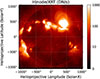 |
Fig. E.1. Hinode/XRT image corresponding to the Flaring Sun DAXSS observation. The colorbar limits are adjusted to enhance visibility of coronal structures that are faint relative to the ongoing flares. |
Appendix F: Close-up of flaring region on the Flaring Sun Hinode/XRT image
Figure F.1 shows a zoom-in on the flaring regions observed by Hinode/XRT during the Flaring Sun observation (2022 April 25). The figure illustrates the correspondence between spectrally derived coronal components and regions identified in imaging-based catalogs. Pixels are color-coded according to the coronal region types identified in Sect. 3.4. Their filling factors were derived from the spectral fit in Sect. 3.3.2: active regions (AR; green), cores (CO; orange), and flares (FL; blue). The contours correspond to active regions (AR (XRT seg.); black) and bright points (BP (XRT seg.); red), from the Hinode/XRT segmentation database (Adithya et al. 2021). Bounding boxes marking flares (FL (HEK); black) and active regions (AR (HEK); blue) detected by multiple solar instruments and registered in the HEK (Hurlburt et al. 2012) are also shown.
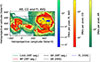 |
Fig. F.1. Zoom-in to flaring regions on the Hinode/XRT image taken during the Flaring Sun observation shown in Fig. 11, showing pixels color-coded by coronal regions (Sect. 3.4) whose filling factors were determined from spectral fitting in Sect. 3.3.2: AR (green gradient), CO (orange gradient), and FL (blue-teal gradient). The black and red contours correspond to active regions (AR (XRT seg.)) and bright points (BP (XRT seg.)), respectively, as identified in the Hinode/XRT segmentation database (Adithya et al. 2021). The flares (FL (HEK)) and active regions (AR (HEK)) simultaneously detected by various solar instruments and registered in the HEK (Hurlburt et al. 2012) are shown as black and blue bounding boxes, respectively. |
All Tables
Elemental abundances for quiescent and flaring solar conditions measured with respect to the Feldman (1992) coronal standard.
All Figures
|
Fig. 1. EMDs of BKC, AR, CO, and FL-AVG regions as described in Sect. 1. The y-axis shows the emission measure per unit area, in units of 1044 cm−5. All EMDs shown here represent time-averaged distributions constructed from multiple snapshots of flares or other types of regions. |
| In the text | |
|
Fig. 2. EMDs of C5.8, M1.0, M1.1, M2.8, M4.2, M7.6, and X1.5 flares as presented by Reale et al. (2001) (individual colors) along with their weighted average EMD (FL-AVG, blue). The y-axis shows the emission measure per unit area, in units of 1044 cm−5. |
| In the text | |
|
Fig. 3. GOES X-ray flux in 1–8 Å band (green) and DAXSS count rates for April 25, 2022 and June 29, 2022. Horizontal gray lines demarcate the GOES flare classes A, B, C, M, and X. The epochs of the DAXSS spectra selected for analysis in this paper are marked in the DAXSS light curve as blue crosses, and vertical dashed lines indicate the one-hour exposure time of the spectra. The Hinode/XRT synoptic images used to verify the SaXS method correspond to the time period indicated by the vertical pink band. |
| In the text | |
|
Fig. 4. DAXSS spectra corresponding to the lowest and highest count rates in the DAXSS light curve along with arbitrarily scaled SaXS models of the various types of coronal regions. This demonstrates the steeper slope of the solar spectra compared with the spectrum of all types of coronal region which indicates an over-contribution of low-signal EM bins (see text in Sect. 3.2). |
| In the text | |
|
Fig. 5. DAXSS spectrum from 29 June, 2022 representing the quiescent Sun fit with APEC-based SaXS models. The model consisting of the AR component alone is shown on the top figure and with the added BKC component is shown on the bottom figure. |
| In the text | |
|
Fig. 6. DAXSS spectrum from 29 June, 2022 representing the quiescent Sun fit with BKC and AR models with variable abundances (VAPEC). |
| In the text | |
|
Fig. 7. DAXSS spectrum from 25 Apr. 2022, representing the Flaring Sun with FL-AVG alone (top), FL-AVG + CO (middle), and FL-AVG + CO + AR (bottom), all using APEC-based SAXS models. |
| In the text | |
|
Fig. 8. DAXSS spectrum from 25 Apr., 2022 representing the flaring Sun fit with AR, CO, and FL-AVG models with variable abundances (VAPEC) for AR and CO and nonequilibrium ionization (VNEI) for FL-AVG. |
| In the text | |
|
Fig. 9. Hinode/XRT images corresponding to quiescent- and flaring-Sun DAXSS observations (top and bottom panels, respectively). |
| In the text | |
|
Fig. 10. Hinode/XRT image during quiescent-Sun observation with highlighted pixels showing the AR component (green gradient) (Sect. 3.4) identified from spectral fitting in Sect. 3.3.1. The solar-limb boundaries, shown by the green circles, are taken from the Hinode/XRT segmentation maps. The inner boundary defines the reference area used in the filling-factor calculations. The black and red contours correspond to active regions and bright points, respectively, as identified in the Hinode/XRT segmentation database (Adithya et al. 2021). The active regions simultaneously detected by various solar instruments and registered in the HEK (Hurlburt et al. 2012) are shown as black bounding boxes. |
| In the text | |
|
Fig. 11. Hinode/XRT image taken during the flaring-Sun observation, showing pixels color-coded by coronal regions (Sect. 3.4) whose filling factors were determined from spectral fitting in Sect. 3.3.2: AR (green gradient), CO (orange gradient), and FL-AVG (blue–teal gradient). The solar limb boundaries (Limb (XRT seg.)), shown by the green circles, are taken from the Hinode/XRT segmentation maps. The inner boundary defines the reference area used in the filling factor calculations. The black and red contours correspond to active regions (AR (XRT seg.)) and bright points (BP (XRT seg.)), respectively, as identified in the Hinode/XRT segmentation database (Adithya et al. 2021). The flares (FL (HEK)) and active regions (AR (HEK)) simultaneously detected by various solar instruments and registered in the HEK (Hurlburt et al. 2012) are shown as black and blue bounding boxes, respectively. |
| In the text | |
|
Fig. A.1. Composite SaXS spectral models made with XSPEC (colored) and their individual APEC components (grey) for the main solar coronal region types used in the SaXS method (see Sect. 2). Colors indicate the coronal region type: red for the background corona (BKC), purple for the active regions (AR), yellow for the cores (CO), and blue for the averaged flares (FL-AVG). |
| In the text | |
|
Fig. C.1. Emission measure distributions of the BKC, AR, CO and FL-AVG regions as described in Sect. 1. The opaque lines are the restricted distributions we use in this paper (described in Sect. 3.2), and the transparent lines show those parts of the original Yohkoh/SXT EMDs that we have discarded. The original EMDs are thus the combination of the opaque and transparent bins, and are also shown in Fig. 1. |
| In the text | |
|
Fig. D.1. Comparison between composite SaXS spectral models in XSPEC derived from the full (solid lines) and restricted (dashed lines) emission measure distributions for the main coronal region types defined in Sect. 3.2. Colors indicate the region type: red for the background corona (BKC), purple for active regions (AR), yellow for cores (CO), and blue for the averaged flares (FL-AVG). |
| In the text | |
|
Fig. E.1. Hinode/XRT image corresponding to the Flaring Sun DAXSS observation. The colorbar limits are adjusted to enhance visibility of coronal structures that are faint relative to the ongoing flares. |
| In the text | |
|
Fig. F.1. Zoom-in to flaring regions on the Hinode/XRT image taken during the Flaring Sun observation shown in Fig. 11, showing pixels color-coded by coronal regions (Sect. 3.4) whose filling factors were determined from spectral fitting in Sect. 3.3.2: AR (green gradient), CO (orange gradient), and FL (blue-teal gradient). The black and red contours correspond to active regions (AR (XRT seg.)) and bright points (BP (XRT seg.)), respectively, as identified in the Hinode/XRT segmentation database (Adithya et al. 2021). The flares (FL (HEK)) and active regions (AR (HEK)) simultaneously detected by various solar instruments and registered in the HEK (Hurlburt et al. 2012) are shown as black and blue bounding boxes, respectively. |
| In the text | |
Current usage metrics show cumulative count of Article Views (full-text article views including HTML views, PDF and ePub downloads, according to the available data) and Abstracts Views on Vision4Press platform.
Data correspond to usage on the plateform after 2015. The current usage metrics is available 48-96 hours after online publication and is updated daily on week days.
Initial download of the metrics may take a while.