| Issue |
A&A
Volume 708, April 2026
|
|
|---|---|---|
| Article Number | A201 | |
| Number of page(s) | 17 | |
| Section | Interstellar and circumstellar matter | |
| DOI | https://doi.org/10.1051/0004-6361/202558050 | |
| Published online | 08 April 2026 | |
Formaldehyde as a densitometer and thermometer in Cygnus-X, the GLOSTAR pilot region, and M8
Utilizing the H2CO ground-state transition
1
Max-Planck-Institut für Radioastronomie,
Auf dem Hügel 69,
53121
Bonn,
Germany
2
Max-Planck-Institut für Extraterrestrische Physik,
Giessenbachstrasse 1,
85748
Garching,
Germany
3
Max Planck Institut für Astronomie,
Königstuhl 17,
69117
Heidelberg,
Germany
4
Purple Mountain Observatory, and Key Laboratory of Radio Astronomy, Chinese Academy of Sciences,
10 Yuanhua Road,
Nanjing
210023,
PR China
★ Corresponding author: This email address is being protected from spambots. You need JavaScript enabled to view it.
Received:
10
November
2025
Accepted:
19
February
2026
Abstract
Context. Measurements of the physical conditions in molecular clumps are key to our understanding of star formation. Formaldehyde (H2CO) is a prevalent molecule in these regions, and it can be used as a diagnostic of the physical conditions.
Aims. Here we explore a technique for determining the volume density and gas kinetic temperature in molecular clumps across various evolutionary phases and environments. The ground-state transition of H2CO has a critical density of ncrit ∼ 104 cm−3, allowing us to use this molecule as a densitometer at n ≤ 105 cm−3and to lessen the discrepancy between the measurements between gas densities derived from molecular tracers and those derived from dust observations.
Methods. The clumps in our study were observed with the IRAM 30-m telescope, marking the first extensive survey of the H2CO (10,1 − 00,0) line across a large sample of sources. These observations were complemented by the H2CO J = 3 − 2 lines, obtained using the APEX telescope. These clumps have been surveyed in three regions, the Cygnus-X giant molecular cloud complex, the GLOSTAR pilot region covering the Galactic plane at longitudes 28° ≤ l ≤ 36°, and the molecular cloud associated with the HII regions in the Lagoon nebula (M8).
Results. We analyzed a total of 127 clumps, including 78 from Cygnus-X, 12 from the GLOSTAR pilot region, and 37 from M8. We derived the gas kinetic temperature, volume densities and H2CO column densities using radiative transfer modeling with pyradex+emcee in 102 clumps. We reproduced the observed line intensities in the sources with volume densities n(H2) = 5.4 × 10⁴−3.8 × 105 cm−3, gas kinetic temperatures Tgas = 16−219 K, and H2CO column densities N(H2CO) = 6.0 × 10¹² −1.6 × 1015 cm−2.
Conclusions. The gas kinetic temperatures obtained from the non-local thermodynamic equilibrium (LTE) modeling with pyradex+emcee agree well with the LTE gas kinetic temperature obtained from the ratio of H2CO (30,3 − 20,2) and H2CO (32,1 – 22,0) lines at densities n(H2) ≤ 105.5 cm−3. However, we find that, at higher densities, LTE temperatures derived from this ratio are over-estimated by up to 0.5 dex. The volume densities we measured are consistent with the volume densities obtained from dust continuum measurements, thereby probing the bulk of the gas. Furthermore, we find that the volume densities and dust temperatures increase with increasing evolutionary phase. The newly available ground-state transition of H2CO allows the physical conditions in various phases of star formation to be constrained more effectively.
Key words: astrochemistry / stars: formation / ISM: abundances / evolution / ISM: molecules / submillimeter: ISM
Member of the International Max Planck Research School (IMPRS) for Astronomy and Astrophysics at the Universities of Bonn and Cologne.
Karl M. Menten was unable to witness the completion of this article, having passed away. Nonetheless, his vital contributions to our project remain deeply valued and will always be remembered.
© The Authors 2026
 Open Access article, published by EDP Sciences, under the terms of the Creative Commons Attribution License (https://creativecommons.org/licenses/by/4.0), which permits unrestricted use, distribution, and reproduction in any medium, provided the original work is properly cited.
This article is published in open access under the Subscribe to Open model.
Open Access funding provided by Max Planck Society.
1 Introduction
The physical and chemical conditions during high-mass star formation are poorly understood (see e.g. McKee & Tan 2002; McKee & Ostriker 2007; Krumholz & Bonnell 2009; Tielens 2021). The formation of massive star clusters in particular is believed to take place in dense (n(H2) > 105 cm−3) and cold clumps (Tkin < 20 K) within molecular clouds (e.g. Pillai et al. 2011). Knowing the initial conditions of star formation prevailing in these regions can shed light on the formation mechanisms of their stellar content (Girichidis et al. 2020). Molecular clouds are the largest structures (≥10 pc) from which gas fragments into clumps (size ∼1 pc), cores (size ~0.05−0.1 pc), envelopes (size ∼300 − 3000 AU) and disks (size ∼10−200 AU) (Pokhrel et al. 2018), eventually accreting onto protostars.
Previous studies have attempted to probe the volume density and kinetic gas temperatures using various molecular tracers, but these methods have limitations. Ammonia (NH3) inversion lines have been used to determine the gas kinetic temperature (e.g. Walmsley & Ungerechts 1983; Tafalla et al. 2004; Wienen et al. 2012), but the NH3 abundance is strongly affected by dust evaporation (Yamato et al. 2022; Redaelli et al. 2023). To probe temperature, CH3CCH, CH3CN, and CH3OH have been used, with CH3OH also being sensitive to density (Giannetti et al. 2017; Lin et al. 2022). The K-level population of CH3OH is sensitive to the gas temperature (e.g. Cummins et al. 1983; Remijan et al. 2004). Higher J-lines of CH3OH trace kinetic temperatures, and lower J-lines trace density in low-, intermediate-, and high-mass star-forming regions (Leurini et al. 2004, 2007). Notably, CH3CN traces hot core temperatures, thus limiting its ability to measure temperatures in cold regions.
Formaldehyde (H2CO) is a ubiquitous molecule believed to form through successive hydrogenation of CO on icy grain mantles (e.g. Mangum et al. 1990; Watanabe & Kouchi 2002; Woon 2002; Yan et al. 2019) or through the gas-phase reaction of CH3 with atomic oxygen (e.g. Potapov & Garrod 2024; Punanova et al. 2025). Indeed, Downes et al. (1980) revealed the presence of this molecule via absorption measurements toward numerous HII regions. The H2CO molecule is a slightly asymmetric rotor molecule that has shown its usefulness in determining the volume density and gas kinetic temperature in a variety of sources due to the collisionally governed K-levels (e.g. Mangum & Wootten 1993; Mangum et al. 2013; Ao et al. 2013; Okoh et al. 2014; Tang et al. 2018, 2021a; Gieser et al. 2021).
Due to the line’s frequency (72.838 GHz) at the lower end of the receiver coverage of the 3/4 mm atmospheric window, only a limited amount of observations have been made of the 10,1 − 00,0 ground-state transition of para-H2CO (hereafter H2CO). Figure 1 shows how the H2CO (30,3 − 20,2)/(10,1 − 00,0) and H2CO (32,1 −22,0)/(30,3 − 20,2) ratios depend sensitively on temperature and density. This line, first detected in the interstellar medium by Akabane et al. (1974; see also Kaifu et al. 1975), has a relatively low critical density of ncrit ∼ 104 cm−3. This property allows the molecule to be used as a densitometer at n ≤ 105 cm−3, as it can also trace the envelopes of clumps, which exhibit a distinct physical behavior from the cores, thereby offering a more comprehensive view of how density, its spatial distribution, and the temperature vary with evolutionary stage across different spatial scales. Studies have shown that the ground-state transitions of ortho-H2CO (11,0 − 11,1) and (21,1 − 21,2) at 6 and 2 cm, respectively, are density tracers (e.g. Mangum et al. 2008; Ginsburg et al. 2011, 2015; Gong et al. 2023). Tang et al. (2017) observed that the fractional abundance of H2CO remains relatively stable across different phases of star formation. The fractional abundance with respect to H2 of H2CO varies by only one order of magnitude during these different phases, with X(H2CO) ≃ 10−10 (Tang et al. 2018).
Previous studies have revealed a significant discrepancy between gas densities derived from molecular tracers and those derived from dust observations. For example, studies using CS (Beuther et al. 2002) or higher J transitions of H2CO (Tang et al. 2018) find higher gas densities compared to dust-based estimates. This discrepancy can be attributed to the high critical densities of the lines used in these studies. The H2CO ground-state transition, H2CO (10,1 − 00,0), now offers a lower critical density line to probe the bulk material of the clumps. This ground-state transition increases the diagnostic utility of H2CO emission lines as tracers of both temperature and density, enabling the probing of lower-density regions (see Fig. 1).
In this paper, we measure the volume density and gas kinetic temperature using H2CO toward a sample of sources in the Cygnus-X star-forming region, the GLOSTAR pilot region, and the Messier 8 (M8) region. The combination of rotational transitions with different critical densities allowed us to probe a large range of gas physical conditions. The paper is organized as follows: in Sect. 2, we present the details of the target sources. In Sect. 3, we present the observations and data reduction. In Sect. 4, we analyze the averaged spectra to determine whether different H2CO transitions are probing the same regions within the clumps. In Sect. 5, we describe the pyradex+emcee methodology and analysis. In Sect. 6, we discuss the obtained gas kinetic temperatures, volume densities, and H2CO column densities, and we explore the physical conditions across the evolutionary phases. Finally, in Sect. 7, we present our conclusions.
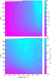 |
Fig. 1 Line-ratios of H2CO (30,3 − 20,2)/(10,1 − 00,0) (top) and H2CO (32,1 − 22,0)/(30,3 − 20,2) as a function of volume densities and gas kinetic temperature computed from pyradex. Bottom plot shows the “bump” at n(H2) ≥ 105.5 cm−3, discussed in Sect 6.1. |
2 Source selection
This study focuses on three specific regions: Cygnus-X (as part of the CASCADE project), the GLOSTAR pilot region, and M8. The following section gives an overview of the three target regions.
2.1 Cygnus allscale survey of chemistry and dynamical environments
Cygnus-X is a nearby (d ∼ 1.5 kpc, Rygl et al. 2012) high-mass star-forming region with OB associations illuminating the cloud complex from the south-west (Knödlseder 2000; Beerer et al. 2010; Wright et al. 2015). Star formation is triggered by strong stellar winds, and several clouds are interacting with their ambient HI envelope specifically in the DR21 filament, with clumps at different evolutionary phases along the structure (Motte et al. 2007; Schneider et al. 2010; Hennemann et al. 2012; Schneider et al. 2023). Recently, a survey using the NOrthern Millimeter Array (NOEMA) and the IRAM 30-m telescope has been conducted with the goal to unveil and connect the chemical and dynamical structures of star formation across a wide range of spatial scales, namely Cygnus Allscale Survey of Chemistry and Dynamical Environments (CASCADE) (Beuther et al. 2022). Motte et al. (2007) and Cao et al. (2019) studied several regions in Cygnus-X, and, in this work, 72 clumps have been targeted. These clumps have masses in the range of ∼1 × 10⁴ – 2 × 10⁶ M⊙, and represent sources in a variety of evolutionary phases from starless clumps to HII regions (Motte et al. 2007; Cao et al. 2019). The observed positions are shown in Fig. 2a and listed in Table A.1.
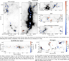 |
Fig. 2 Locations of clumps in Cygnus-X (top), the GLOSTAR pilot region (bottom left), and M8 (bottom right). |
2.2 Global view on star formation in the Milky Way - Pilot region
The GLObal view on Star Formation in the Milky Way (GLOSTAR) project aims to characterize the unbiased statistical properties of star formation in the Galactic plane (for an overview, see Brunthaler et al. 2021). The GLOSTAR survey uti-lizes the Jansky Very Large Array (VLA; Perley et al. 2011) and the Effelsberg 100-m telescope1 to conduct continuum observations covering the frequency range of 4–8 GHz. In addition, the survey includes simultaneous observations of the 6.7 GHz CH3OH maser line, various radio recombination lines (RRL), and notably the 4.8 GHz H2CO absorption line. The “GLOSTAR pilot region” of this survey, discussed by Brunthaler et al. (2021), covers 28° < l < 36°, |b| < 1°) and its radio continuum emission is shown in Fig. 2b. This 16 square-degree pilot region shows a diversity of extended and compact sources, including HII regions, supernova remnants, and several CH3OH masers (Medina et al. 2019; Dokara et al. 2021; Nguyen et al. 2022; Dokara et al. 2023). We observed positions in the GLOSTAR pilot region toward which H2CO absorption was observed in the survey. These are shown in Fig. 2b and listed in Table A.2.
We determined the distance using the radial velocity of the GLOSTAR sources, although this is challenging due to the kinematic velocity distance ambiguity discussed thoroughly in Roman-Duval et al. (2009). We utilize the Parallax-Based Distance Calculator2 for the GLOSTAR sources, as described in Reid et al. (2019). In the case of G29.95 0.01 and G31.27+0.06, we adopt the trigonometric parallax −distances measured by Zhang et al. (2014). The distances are listed in Table A.2.
Transitions of H2CO observed with the IRAM 30-m and the APEX 12-m telescopes.
2.3 Messier 8
The Lagoon Nebula, also known as Messier 8 (M8 hereafter), is a bright HII region illuminated by O- and B-stars. Located at a distance of 1.3 kpc, it is one of the nearest HII regions, characterized by a high UV flux (Damiani et al. 2017; Tiwari et al. 2019). Tothill et al. (2002) identified clumps associated with the molecular cloud. A plethora of molecules are identified in the M8 photodissociation region and 38 dense dusty clumps that surround it, some of which also show photodissociation region signatures, while 38% are likely hosting protostellar objects (Kahle et al. 2024). The clumps in the M8 region were found to have dust temperatures, Tdust, ranging from 15.7 to 43.2 K, and H2 column densities, N(H2), ranging from 6.7 × 10²¹ to 6.1 × 1022 cm−2. Kahle et al. (2024) suggest that the remnant gas in the M8 region may be fragmenting due to the radiation pressure of the surrounding O- and B-stars. The data for four H2CO transitions from 37 clumps within the M8 region in this study were reduced and analyzed by Kahle et al. (2024). The locations of the clumps can be seen in Fig. 2c with positions listed in Table A.3.
In order to determine volume densities, gas kinetic temperatures and H2CO column densities using a consistent method, we combined data from all three regions. The considered clumps span a wide range of distances, molecular cloud conditions, kinematics, and evolutionary phases. This diversity allowed us to apply our method across a variety of environments, thereby enhancing the robustness of our analysis.
2.4 Comparison sample
The APEX Telescope Large Area Survey of the GALaxy (ATLASGAL) provided a large inventory of ~10 000 dense clumps within the inner Galactic region (Schuller et al. 2009). We compare our results, presented in Appendix C with measurements from the ATLASGAL clumps; sources representative of high-mass clumps in our inner Galaxy at different evolutionary phases (Urquhart et al. 2018).
A sub-sample of 110 clumps, namely the “ATLASGAL Top 100”, is designed to contain sources that represent different evolutionary phases of high-mass star formation: starless/prestellar, mid-infrared weak cores, mid-infrared bright cores, and HII regions (König et al. 2017). The ATLASGAL selected TOP 100 sources probe the clumps on the scales of 0.12–1.95 pc (Csengeri et al. 2014; König et al. 2017; Tang et al. 2018), similar to that probed in this study (0.18–1 pc for all three regions). Tang et al. (2018) determined the volume density and gas kinetic temperatures using H2CO (30,3 − 20,2), (32,2 − 22,1), (32,1 − 22,0), (40,4 − 30,3), (42,3 − 32,2), and (42,2 − 32,1). This study and Tang et al. (2018) both utilize the three J = 3−2 H2CO transition, listed above. However, this study additionally used the J = 1 − 0 transition, allowing us to study the lower density material, while Tang et al. (2018) used J = 4 − 3.
3 Observations
We observed several H2CO transitions toward molecular clumps in the Cygnus-X, GLOSTAR, and M8 regions described in Sect. 2. An overview of the targeted H2CO transitions and their detection rates is presented in Table 1.
3.1 IRAM 30-m telescope observations with EMIR 090
We conducted observations with the Institut de Radioastronomie Millimétrique (IRAM; Baars et al. 1987) 30-m telescope, located on the Pico Veleta in the Spanish Sierra Nevada. We used this telescope to observe the ground-state H2CO (J = 1 − 0) transition. For these observations, we employed the Eight Mixer Receiver (EMIR3; Carter et al. 2012) and the Fourier Transform Spectrometer FTS200 as backend, which provides a channel width of 195 kHz (corresponding to a velocity interval, ∆υ, of 0.80 km s−1). At the line’s rest frequency, 72.8 GHz, the telescope’s FWHM beam width is ≈33′′.
Cygnus-X was mapped as part of the CASCADE program (Project ID: 145-19 and 031-20; PIs: F. Wyrowski and H. Beuther, Beuther et al. 2022). Observations of the GLOSTAR sources were carried out with the IRAM 30-m telescope on 2016 May 28th and 29th (Project ID: 110-15; PI: H. Nguyen). A bandwidth of 8 GHz per sideband was employed, providing a total frequency coverage of 16 GHz across the Cygnus-X and GLOSTAR sources, specifically 70.2–78.2 GHz in the lower sideband and 85.9–93.9 GHz in the upper sideband. The IRAM 30-m telescope observations of the 72.8 GHz H2CO ground-state line toward the Cygnus-X sources used on-the-fly mapping. The spectrum of each clump is extracted from a region matching the angular resolution of ∼33′′. The telescope pointing and focus were checked with Mars and 1741−038 for the Cygnus-X and GLOSTAR sources, respectively. The clumps in M8 were observed during several runs between 2022 March and June (Project ID: 141-21; PI: F. Wyrowski). The M8 sources were covered as part of a spectral line survey by Kahle et al. (2024), covering a frequency range of 40.3 GHz between 70 and 117 GHz, for which the FWHM beam size varies between 34′′ and 21′′. The FWHM beam width of the IRAM 30-m telescope4 θB, in arcseconds, is given by 2460/ν, where ν is the observed frequency in GHz.
We converted the observed corrected antenna temperatures,  , which assumed a forward efficiency, ηeff, of 0.95, to main beam temperatures, TMB, using a main-beam efficiency, ηMB, that depends on the observing frequency5. At 72.8 GHz, the frequency of ground-state H2CO line, ηeff = 0.79.
Parameters of the IRAM and APEX observations.
3.2 APEX observations with nFLASH230
The H2CO (J = 3−2) observations were performed using the 12-m Atacama Pathfinder EXperiment (APEX) telescope (Güsten et al. 2006), located on the Chajnantor plateau in the Atacama desert (Güsten et al. 2006). We carried out single-pointing observations toward the selected 72 clumps in Cygnus-X during 2022 July and August (project ID: M-0109.F-9508C-2022; PI: Ivalu Barlach Christensen) and 10 clumps in the GLOSTAR pilot region during 2024 April and May (project ID: M-099.F-9519A-2017; PI: H. Nguyen and I. B. Christensen). We made use of the nFLASH 230 receiver, tuning the lower sideband (LSB) to 217.538 GHz to cover three H2CO lines (30,3 − 20,2, 32,2 − 22,1, and 32,1 − 22,0, see Table 1 for the summary of spectral line properties) for clumps in Cygnus-X and the GLOSTAR pilot region. The observations were performed in position switching mode, with selected clean reference positions for each sub-regions within Cygnus-X and a fixed offset of (+600′′, 0) for each source in the GLOSTAR pilot region. The telescope focus and pointing were checked, depending on the day, with Mars, Jupiter, or Saturn, achieving an estimated pointing accuracy of ∼5′′. The frequency range coverage was 200.4–208.4 GHz in the lower sideband and 216.4–224.4 GHz in the upper sideband, with a typical integration time of 5 minutes. However, the five clumps in Cygnus-X DR20 have additional observations of 30 minutes each. Additional integrations were performed for clumps in which the strongest H2CO (30,3 − 20,2) line was observed but the fainter H2CO (32,2 − 22,1) and H2CO (32,1 − 22,0) lines were not detected above 4σ. An overview of the reference positions is presented in Appendix A. An in-depth description of observations and data processing in the spectral survey of M8 is presented in Kahle et al. (2024) (project-ID: M-0107.F-9530C-2021; PI: Karl M. Menten). The frequency coverage of the spectral line survey in M8 clumps spans 58.3 GHz between 210 and 280 GHz.
We converted the APEX TA∗ scale to a TMB scale using ηeff = 0.95 and a main-beam efficiency depending on the date of observations. In the case of Cygnus-X sources, observations of Mars, Jupiter, and Saturn allowed us to estimate the beam efficiencies from observations, and we found 0.68 < ηMB < 0.86. Based on Mars observations, we found ηMB = 0.77 for the GLOSTAR sources. For the M8 sources, ηMB = 0.80 was adopted based on Jupiter6. An overview of the receiver tuning parameters of the observations of the three sub-samples is presented in Table 2.
We applied a beam correction factor of  to account for the difference in beam sizes. The observations were conducted with the IRAM and APEX telescopes, which were chosen because their beam sizes are comparable, thereby minimizing systematic uncertainties introduced by beam mismatch.
3.3 Data processing of spectroscopic data
All data of observed transitions of H2CO were reduced using the Grenoble Image and Line Data Analysis Software (GILDAS) software developed by IRAM7 (Pety 2018). The spectrum of each H2CO transition for each clump in CASCADE was produced using the Continuum and Line Analysis Single-dish Software (CLASS). All spectra were smoothed to a spectral resolution of the H2CO (10,1 − 00,0) line, that is, 0.8 km s−1. For each H2CO line, the spectrum of every source is centered on the source’s systemic LSR velocity, υLSR, and covers a span of 160 km s−1, υLSR ± 80 km s−1. This method of data processing was performed on Cygnus-X and GLOSTAR sources. The data processing of M8 is described in Kahle et al. (2024).
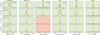 |
Fig. 3 Spectra of the four H2CO transitions toward six clumps, two from each region. The background color indicates whether a line is at ≥4σ (green) or <4σ (red). The dashed black line indicates the peak velocity of the fit Gaussian for each transition. Examples of clumps with too few lines (N33), differences in ∆υ (N46), or a double peak (G28.28–0.36) are shown. |
4 Results
Using data from the IRAM 30-m and APEX 12-m telescopes, we investigated in detail the H2CO emission lines observed toward the clumps in Cygnus-X (78 sources), GLOSTAR (12 sources), and M8 (37 sources). We first fit Gaussian line profiles to the spectra of these clumps as input for the subsequent analysis of the physical conditions in the gas.
4.1 Spectral analysis
We analyzed the spectra of each clump focusing on the H2CO (10,1 −00,0), (30,3 −20,2), (32,2 −22,1), and (32,1 − 22,0) lines. We utilized the Gaussian fitting procedure of CLASS to obtain the integrated intensity, ∫ TMB, peak main-beam brightness temperature TMB, velocity of peak emission, υpeak, and linewidth at the full width at half maximum (FWHM), ∆υ. In the case of clumps with several velocity components, as indicated in Fig. 2, a single Gaussian was fit to each velocity component. These clumps are indicated with “A” and “B” in Appendix B. The maximum number of velocity components is two for a single clump. Six sources in Cygnus-X and two sources in the GLOSTAR pilot region were found to have two velocity components.
Figure 3 shows example spectra of all the H2CO lines and the Gaussian fit results for two sources each in Cygnus-X, the GLOSTAR pilot region, and the M8 region. The line parameters for the Cygnus-X, the GLOSTAR pilot region, and the M8 region sources are presented in Appendix B. A detailed description of the analysis can be found in Sect. 5.1. The parameters obtained for our Cygnus-X, GLOSTAR pilot region, and M8 sources are presented in Appendix B.
4.2 Detection rates
To estimate the H2 volume density, gas kinetic temperature, and H2CO column density, we required at least three emission lines to be detected for each clump. With a detection criterion of ≥4σ, the highest detection rates of the formaldehyde lines are the ground-state transition H2CO (10,1 − 00,0) and H2CO (30,3 −20,2) (Eup/k = 3.50 K and Eup/k = 20.96 K, respectively). These two emission lines are observed in all 72 clumps in Cygnus-X and ten clumps in the GLOSTAR pilot region. Of these 72 clumps in Cygnus-X, six clumps exhibit two velocity components, resulting in 78 H2CO measurements. In the GLOSTAR pilot region, eight of the ten clumps have a single velocity component, while 2 have an additional velocity component. Despite possibly originating from the same source, each velocity component is treated as if originating in a separate clump.
The detection rates for Cygnus-X, the GLOSTAR pilot region, and M8 are summarized in Table 1. High detection rates (>80%) of the weaker H2CO transitions (i.e., 32,2 − 22,1 and 32,1 − 22,0) are observed in both Cygnus-X and GLOSTAR clumps. In Cygnus-X, all four H2CO lines are detected above 4σ in 60 sources. Of the remaining ten clumps, these two strong lines are detected along with either 32,2 − 22,1 in five sources or 32,1 − 22,0 in the other five. In the GLOSTAR pilot region, all ten clumps show all four lines above 4σ.
In contrast, M8 shows lower detection rates across all four transitions. The stronger lines are detected in 95% of sources, while the weaker H2CO (32,2 − 22,1) and (32,1 − 22,0) transitions are detected in only 49% and 65% of clumps, respectively. Of the 37 M8 clumps observed, 13 were excluded from further analysis due to having fewer than three detected H2CO transitions.
The high detection rates of H2CO (10,1 − 00,0) and (30,3 − 20,2) across all regions suggest the abundant nature of H2CO in the clumps. The different, and lower, detection rates of the higher excitation lines reveal the underlying excitation conditions (e.g. density and temperature) of these regions, which we investigate further.
4.3 Line parameter comparisons
We examined the line profile of each transition for every clump in Cygnus-X, the GLOSTAR pilot region, and M8 to ensure consistency. Based on comparison of the peak velocity, υLSR, and linewidth, ∆υ, of each measurement, we confirm that all lines are probing similar gas components within each clump.
Figure 4 shows the difference in peak velocity between the four transitions (top), and the linewidth comparison of the four transitions (bottom). The green shaded areas in Fig. 4 indicate the regions of the accepted range. Both of the accepted ranges the υLSR and ∆υ are based on the spectral resolution of 0.8 km s−1. The accepted range for the difference between υpeak is ±0.8 km s−1, and for the difference between ∆υ, the range is ±3 × 0.8 km s−1. The peak velocities are obtained by fitting a Gaussian for each H2CO transition (see Sect. 4.1). Each J = 3−2 transition’s peak velocity is compared with the peak velocity of H2CO (10,1 − 00,0). None of the sources in Cygnus-X, GLOSTAR, and M8 are discarded, as all lines are aligned. Similar linewidths further ensure that the transitions originate from the same gas component. Similar to the peak velocity comparison, we also compare the linewidths of J = 3 2 with the strongest transition H2CO (10,1 − 00,0). Sources with a linewidth different than ∆υ(H2CO (10,1 − 00,0)) are discarded. Two sources in Cygnus-X and none in the GLOSTAR pilot region and M8 region are discarded due to the difference of linewidths.
H2CO (32,2 − 22,1) and H2CO (32,1 − 22,0) are expected to exhibit similar emission line profiles, as their values for Eup and Aij are identical (see Table 1 for reference, Müller et al. 2001). If, as one expects, these transitions originate under the same physical conditions, their line integrated intensities should be comparable. This comparison is shown in Fig. 5, which plots the intensities of the two transitions from the three different regions in this study: within the uncertainties, the integrated intensities of both lines are identical.
To summarize, we discarded sources based on the following criteria: fewer than three lines detected, misaligned velocities within a source, differing linewidths among transitions, and insufficient agreement between line intensities of the H2CO (32,2 − 22,1) and H2CO (32,1 − 22,0) transitions. As a result, a total of 10 sources are discarded in Cygnus-X, none are discarded in the GLOSTAR pilot region, and 13 are discarded in M8. An overview of the sources discarded is presented in Table B.4.
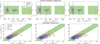 |
Fig. 4 Top row: difference in υpeak between the H2CO (10,1 − 00,0) line and the three higher J-transitions of H2CO. The X (in the y-axis) denotes the υpeak noted in the x-axis. Bottom row: linewidths of the different H2CO transitions. In top and bottom rows, sources in Cygnus-X are shown in purple, GLOSTAR sources in orange, and M8 sources in blue. The black symbols indicate clumps that do not satisfy the velocity criterion (green shaded region) and were excluded from further analysis. |
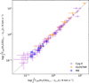 |
Fig. 5 Comparison of H2CO (32,2 − 22,1) and H2CO (32,1 − 22,0) integrated intensities. The sources in Cygnus-X, the GLOSTAR pilot region, and M8 are shown in purple, orange, and blue, respectively. |
5 Analysis
In the following section, we analyze the volume density, gas kinetic temperature and H2CO column density for clumps in Cygnus-X (68 sources), the GLOSTAR pilot region (ten sources), and the M8 region (24 sources). Furthermore, based on the modeled H2 volume densities, the calculation of H2 column densities are described.
5.1 Modeling the physical conditions using H2CO
The goal was to determine the volume density, gas kinetic temperature, and column density of H2CO by comparing the line intensities with a model. We utilize pyradex8 under non-local thermodynamic equilibrium (LTE) conditions, the publicly available Python wrapper for RADEX (van der Tak et al. 2007), in conjunction with the Python package emcee9. The following description outlines the pyradex+emcee analysis approach for a single clump.
The modeled line parameters for a given set of physical conditions are obtained using pyradex. The background temperature, Tbg, taken to be 2.725 K (the temperature of the cosmic microwave background; Fixsen 2009), and the linewidth are assumed to be fixed, and it is assumed that the clump behaves as an expanding sphere so that the radiative transfer can be treated under the local velocity gradient (LVG) assumption. This assumption implies that there are no non-local radiative effects, and that the line-of-sight molecular column density and H2 volume density are independent. The pyradex+emcee modeling assumes an LVG geometry and yields uniformly distributed physical conditions. We adopted a spherical geometry and set the beam filling factor to f = 1 for the modeling, as the beam dilution has been accounted for in the input line intensities. The linewidth was determined as the weighted average of the transitions measured toward the clump, with the condition that the transitions have similar linewidths, indicating that they probe the same gas. The collision rate coefficients for H2CO were adopted from Wiesenfeld & Faure (2013), who calculated them for 21 temperatures in the range from 10 to 300 K. The collisional partners of H2CO were assumed to be p- and o-H2, with an assumed H2 ortho-to-para ratio of 0.01 (Pagani et al. 2009; Dislaire et al. 2012).
The model parameters are p = (n(H2), Tkin, N(H2CO)). We define a Bayesian approach, with the posterior probability distribution (Pr(p|Idata)) of the model parameters p (notation following Yang et al. 2017):
 (1)
(1)
defined in terms of the prior probability Pr(p), the likelihood of the observed intensity of H2CO given the parameter values, Pr(Idata|p), and the probability of the data (commonly referred to as “evidence”), Pr(Idata), serving as a normalizing factor. The likelihood, assuming the noise is independent, is the product of Gaussian probability density functions:
 (2)
(2)
Here, σi is the respective error of the observed intensity of H2CO in  , and
, and  is the respective modeled intensities of H2CO with pyradex. We used the logarithmic form of Eq. (2). To ensure that the parameters remain within reasonable astrophysical conditions while still allowing freedom to explore the parameter space, boundaries are set for the ranges of log(n(H2)/cm3), log(Tkin/K), and log(N(H2CO)/cm2). These boundaries are defined as log(n(H2)) = 0 − 7, log(Tkin) = 1 − 2.47 (constrained by the availability of collisional rate coefficients; see above) and log(N(H2CO)/cm2) = 10 − 17.
We utilized 400 “walkers” to explore the parameter space. We designated a “burn-in” stage consisting of 100 iterations. We used scipy.curve_fit together with pyradex to obtain a preliminary fit of the physical model parameter, generating an initial position in the parameter space. After the first 100 iterations, the initial position of the parameter space was “forgotten”, and the following stage (“walking” stage) consisted of 1000 iterations sampling the posterior distribution.
The H2 volume density, gas kinetic temperature, and H2CO column densities are obtained by the median of the posterior probability distribution for each parameter, and the maximum posterior probability within the 16 and 84% quantiles (= ± 1σmodel). These modeled parameters are presented in Table C.1.
5.2 H2 volume density, gas kinetic temperature, and H2CO abundance
Figure 6 shows the distribution of the H2 volume density, gas kinetic temperature, H2CO column density, and H2CO abundance of sources in Cygnus-X, the GLOSTAR pilot region, and M8. We compared the results of this study with the ATLASGAL Top 100 sources obtained by Tang et al. (2018). We accept the modeled physical parameters with a relative error tolerance of σmodel,rel ≤ 50%, where σmodel is obtained from the posterior distribution. The H2 volume densities comprising sources in Cygnus-X, the GLOSTAR pilot region, and the M8 region, span a range of n(H2) = 5.4 × 10⁴ – 3.8 × 105 cm−3. Figure 1 illustrates how the H2CO (30,3 − 20,2)/(10,1 − 00,0) and H2CO (32,1 − 22,0)/(30,3 − 20,2) ratios, computed with pyradex, vary as a function of H2 volume density and temperature. The gas kinetic temperatures vary within the range of Tgas = 16 219 K, while the H2CO column densities span the range of N(H2CO) = 6.0 × 10¹²−1.6 × 1015 cm−2.
We estimated the H2 column density, with the line-of-sight length, L, assuming a spherical structure of the clumps. The ratio of the column density and volume density yields the line-of-sight scale length
 (3)
(3)
The size of the clumps was taken as the angular resolution, θAPEX = 29′′. To determine the scale length, L, of a source, it is essential to have well-determined distances. The clumps in Cygnus-X have sizes of 0.21 pc, and those of the clumps in the M8 region are 0.18 pc, as the distances to the entire cloud of Cygnus-X and M8 are constant (Rygl et al. 2012; Damiani et al. 2017). The clumps of the GLOSTAR pilot region have varying distances (as described in Sect. 2.2; Reid et al. 2019), resulting in clump sizes spanning 0.26–1.72 pc. Utilizing this H2 column density, we obtained the fractional abundance of H2CO. The mean of X(H2CO) in all three catalogs is ≥10−10 (see the rightmost part of Fig. 6 for the distribution). We obtain H2CO abundances comparable to those in dense cores, photodissociation regions, and cloud scales, ranging from ~10−11 to ∼10−9 (Guzmán et al. 2013; Gerin et al. 2024). We also find H2CO abundances higher than 10−9, in the Cygnus-X region.
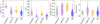 |
Fig. 6 Distribution of (left to right) the H2 volume density, gas kinetic temperature, the H2CO column density, and the fractional abundance. The sources in Cygnus-X, the GLOSTAR pilot region, and M8 are shown in purple, orange, and blue across all distributions, respectively. Similar high-mass sources from the ATLASGAL Top 100, measured using higher J-transitions of H2CO by Tang et al. (2018) are depicted in gray. |
6 Discussion
Here, we discuss the results of all the clumps (102 in total) in the three regions and their obtained physical conditions. We discuss the obtained gas kinetic temperatures and volume densities further in Sects. 6.1 and 6.2.
The higher J-transitions analyzed by Tang et al. (2018) probe higher critical densities, with the critical density of the additional transition (ncrit(H2CO (40,4 – 30,3))~ 106 cm−3) being an order of magnitude higher than that of the highest J-transition used in this study (ncrit(H2CO (10,1 − 00,0)) ∼ 10 cm−3). We find the volume densities of sources in Cygnus-X, the GLOSTAR pilot region, and the M8 region to be an order of magnitude lower than the ATLASGAL sources. Furthermore, the upper levels of the higher J-transitions are higher than that of the J-transitions used in this study. The gas kinetic temperatures are found to be slightly higher, albeit overlapping with some higher temperature clumps in Cygnus-X and GLOSTAR pilot region.
6.1 LTE and non-LTE gas kinetic temperatures
In this section, we present a comparison of the gas kinetic temperature obtained using a non-LTE analysis using pyradex+emcee (described in Sect. 5.1) and Tkin values derived from the H2CO (30,3 − 20,2) to H2CO (32,1 − 22,0) ratio under the LTE assumption. Mangum & Wootten (1993) and Tang et al. (2018) found a dependence of the LTE gas kinetic temperature and the H2CO (30,3 − 20,2) and H2CO (32,1 − 22,0) integrated intensity ratio:
 (4)
(4)
Figure 7 plots the non-LTE gas kinetic temperature versus the H2CO (30,3 − 20,2) and H2CO (32,1 − 22,0) integrated intensity ratio for the sources in our target samples and the ATLASGAL sources discussed by Tang et al. (2018).
The ATLASGAL sources exhibit higher kinetic temperatures compared to the Cygnus-X and M8 sources, but their kinetic temperatures overlap with those sources in the GLOSTAR pilot region (see Fig. 6). The clumps in the GLOSTAR pilot region trace the envelopes of HII regions, and therefore likely trace heated gas. Furthermore, we expanded the relation toward lower temperatures. Tang et al. (2018) discussed that at higher densities, the gas kinetic temperatures exceeding 60 K obtained with this ratio might be overestimated at volume densities of 105−7 cm−3.
The LTE gas kinetic temperatures calculated using Eq. (4) are higher than non-LTE measurements as the volume density increases (see Fig. 8). Tang et al. (2018) discussed a large “bump” in the H2CO (30,3 − 20,2) and H2CO (32,1 − 22,0) line intensity ratios in their temperature-volume density plot (see their Fig. 4). The bump begins at n(H2) ≃ 105.5 cm−3. This bump suggests that for a constant gas kinetic temperature and constant H2CO (30,3 − 20,2) and H2CO (32,1 − 22,0) line intensity ratio, no unique volume densities can be determined. The bump occurs because the H2CO (32,1 − 22,0) line intensity increases more rapidly than the line intensity of H2CO (30,3 − 20,2) for increasing densities n(H2) > 105 cm−3. Tang et al. (2018) noted that the bump becomes more pronounced as the line ratios increase. Thus, the increasing difference between LTE and non-LTE gas kinetic temperature found in Fig. 8 is due to the LTE gas kinetic temperature calculation not accounting for the rapid increase of H2CO (32,1 − 22,0) line compared with H2CO (30,3 − 20,2).
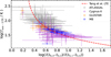 |
Fig. 7 Gas kinetic temperature of sources in Cygnus-X (purple), the GLOSTAR pilot region (orange), and M8 (blue) using pyradex+emcee. The gray points show the temperatures obtained for the ATLASGAL sources by Tang et al. (2018). The dashed red line shows the LTE gas kinetic temperature function presented in Eq. (4). |
6.2 Volume densities
We investigated the obtained volume densities from our set of H2CO lines, and we compared them with the gas densities obtained from dust continuum measurements. Figure 9 shows the comparison between the volume densities obtained from the H2CO emission lines and the 1.2-mm continuum emission, as reported by Motte et al. (2007) for Cygnus-X and by Tothill et al. (2002) for M8. Figure 9 reveals that the regions where the gas and dust are probed overlap with the detection of H2CO. Line emission measurements typically yield higher volume densities compared to dust continuum measurements. This bias occurs because emission lines require specific densities for efficient excitation, while continuum measurements probe all line emissions combined. Beuther et al. (2002) compared volume densities derived from dust continuum data with values determined through the LVG modeling of CS emission. They found that molecular line emission measurements yielded volume densities an order of magnitude larger than those obtained from dust continuum measurements. Given that ncrit(H2CO (10,1 − 00,0)) is 2.8 × 104 cm−3, this line appears well suited for probing the bulk of the gas in massive clumps that have an average H2 density of ∼104 cm−3(Csengeri et al. 2014; Urquhart et al. 2018).
Weaker lines (i.e. 32,2 − 22,1 and 32,1 − 22,0) result in the higher number of clumps discarded in the M8 regions. Kahle et al. (2024) determined the H2 column density from the spectral energy distributions (SEDs) of the clumps. Clumps with the two weaker lines not detected in the M8 region have an order of magnitude lower H2 column densities than clumps analyzed with pyradex+emcee in the M8 region. The clumps M8SC5, M8C2, and M8C3 show particular cases of non-detection in either of the two stronger lines (i.e. 10,1 − 00,0 and 30,3 − 20,2). H2CO (10,1 − 00,0) was not detected at >3σ in M8C2, although a faint line was observed. For the clump M8C3, we did not observe the H2CO (10,1 − 00,0). Only H2CO (10,1 − 00,0) was detected in M8SC5. The remaining J = 3 − 2 transitions could likely not be detected as the IRAM 30-m observations are offset from the APEX observations in the case of M8SC5 (and M8WC3 and M8SE8).
The physical processes contributing to fragmentation during star formation remains an open question. The clump density structure has been proposed to determine the fragmentation (e.g. Pandian et al. 2024). Observations of clumps indicate that clumps form stars at a higher rate that expected from their average spatial densities. This higher rate is proposed to be a result from the dynamic free-fall (e.g. Tan et al. 2006; Parmentier 2020), as seen from the more evolved star-forming regions exhibiting steeper density slopes (Lin et al. 2022).
Conversely, Girichidis et al. (2011) suggests that the density structure of the large-scale clump (inside-out formation process) gives insight to the initial conditions and the fragmentation of the region. Beuther et al. (2024) found that the density structure of clumps is flatter compared to that observed on core scales by Gieser et al. (2021), possibly because the star-forming regions are still embedded within larger-scale structures. Nevertheless, in an attempt to understand the density structures of star-forming regions, constraining the volume density at different scales provides important insights into understanding star formation.
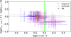 |
Fig. 8 Difference between the gas kinetic temperature of sources in Cygnus-X (purple), the GLOSTAR pilot region (orange), and M8 (blue) using pyradex+emcee compared with the LTE gas kinetic temperature function presented in Tang et al. (2018). The dashed green line marks n(H2) = 105.5 cm−3. |
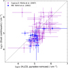 |
Fig. 9 Comparison of volume densities in Cygnus-X (purple) and M8 (blue) obtained with pyradex+emcee and the 1.2-mm continuum emission by Motte et al. (2007) for Cygnus-X and Tothill et al. (2002) for M8. The dashed gray line shows x = y. |
6.3 Physical conditions in different evolutionary stages of clumps
We utilize the method described by Urquhart et al. (2022) to determine the evolutionary phase of each clump in Cygnus-X and the M8 region. The SEDs of the quiescent phase and star-forming clumps can be described as gray body radiation, a modified version of blackbody radiation.
Quiescent clumps are dark at wavelengths of 70 µm or less. As protostellar objects form within clumps, their accretion luminosity warms the envelope, shifting the SED peak to shorter wavelengths. This warming process makes the proto-star detectable first at 70 µm, then at mid-infrared (≤24 µm), and finally at near-infrared wavelengths as it evolves into a young stellar object (YSO). High-mass stars produce significant UV flux, ionizing their surroundings and creating HII regions detectable by compact radio and mid-infrared emission. This gradual evolution in the SED allows the use of carefully selected far- and mid-infrared wavelength images (3.6, 24, and 70 µm) to distinguish between quiescent and star-forming clumps and classify embedded objects.
The Spitzer Legacy Survey of the Cygnus-X Region (Kraemer et al. 2010; Beerer et al. 2010) provides observations of 3.6 and 24 µm emission in Cygnus-X. The Herschel imaging survey of OB Young Stellar objects program (Motte et al. 2010) supplies the 70 µm emission data. The continuum maps of the clumps in Cygnus-X are obtained with MUSTANG-2 camera on the Green Bank Telescope under project GBT22A-280 (Kim et al. 2025).
For the M8 region, we obtain the 3.6 µm and 24 µm emission from archival data of the Spitzer telescope (Carey et al. 2009; Churchwell et al. 2009). We use the AKARI data covering 65 µm, calibrated by Kahle et al. (2024), to estimate the 70 µm emission. The AKARI satellite has a lower spatial resolution than this work (θbeam = 63.4′′; Kahle et al. 2024). We extract the 65 µm emission centered at each clump over the entire beam size. The continuum emission of the M8 region are obtained with the Submillimetre Common-User Bolometer Array (SCUBA; Holland et al. 1999) of the James Clerk Maxwell Telescope10 by Tothill et al. (2002) (see Fig. 2c). Following the approach by Urquhart et al. (2022), we visually examine the evolutionary phases to determine if emission is present at each of these wavelengths. For the 65 µm emission in the M8 region, we rely on the work of Kahle et al. (2024) to decide whether a clump shows detectable emission at 65µm.
We determine the evolutionary phases of clumps for which the physical conditions have been measured. These are in Cygnus-X (66) and clumps in M8 (24). We discard the clumps where the evolutionary phase was ambiguous (2 in Cygnus-X). Fig. 10 shows the distribution of the evolutionary phases of Cygnus-X and M8 clumps. The quiescent phase is the most numerous in the Cygnus-X region. In M8 region, only proto-stellar and HII phases are observed, with the protostellar phase being the most prevalent. The sample in the GLOSTAR pilot regions are all in the HII phase (Brunthaler et al. 2021; Dokara et al. 2021, H. Nguyen priv., comm.).
The determined evolutionary phase in the M8 region identifies two of the 24 clumps as HII regions, while the remaining clumps are classified as protostellar. The clumps, M8HG and M8E (marked in red circle in Fig. 2c), have previously been determined as HII regions (see e.g. Molinari et al. 1998; Tothill et al. 2008). The “S*” clumps in the southern part of M8 are associated with a larger structure known as “the central ridge”, which has been identified as a prominent site of star formation activity (Tothill et al. 2002, 2008). All sources in the central ridge are classified as protostellar. The clumps, designated EC 1–5, lie near the open cluster NGC 6530 (Tothill et al. 2008; Chen et al. 2007), and are also classified as protostellar clumps. The open cluster has triggered star formation in M8E (Tiwari et al. 2020), and M8HG represents one of the most recent starbursts in the M8 region (Arias et al. 2006).
Figure 11 shows the distribution of the H2 volume density, temperature and H2CO fractional abundance with the evolutionary phases in comparison with the ATLASGAL sample (Urquhart et al. 2022) and densities derived with CH3OH of the ATLASGAL Top 100 sample (Giannetti et al. 2025). The three physical parameters are discussed in the following sections.
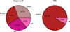 |
Fig. 10 Distribution of the evolutionary phases of the clumps in the Cygnus-X (left) and M8 region (right). “Protost”. denotes protostellar and “Quiesc”. denotes quiescent stage. |
6.3.1 H2 volume density
The left-most plot in Fig. 11 demonstrates an increase in H2 volume density across evolutionary phases, with medians increasing ∼0.5 dex. This increase is particularly significant as it highlights the dynamic processes at play in star formation regions, and reinforces that the density increases with evolutionary phase. Comparatively, the mean H2 volume densities of the ATLAS-GAL sources do not exhibit the increasing trend observed in our sample. Specifically, the H2 volume densities of our sample, spanning from the quiescent to the YSO evolutionary phase, overlap with those of the ATLASGAL sources. While some overlap occurs at the HII phase, our sample generally shows higher volume densities. Similarly, the H2 volume densities of the ATLASGAL Top 100, derived from CH3OH observations, increase as the clumps evolve (Giannetti et al. 2025). These densities generally exceed those derived for our source sample, potentially because CH3OH is tracing higher densities.
Theoretical models predict such an increase in H2 volume density as gas continuously accretes onto clumps throughout the four phases (e.g. Shu et al. 1987; Offner et al. 2022). Observationally, Lin et al. (2022) observed that clumps becomes denser with increasing evolutionary phase. For instance, during the initial phases of star formation, the gravitational collapse of molecular clouds leads to the formation of denser regions where material can accumulate. The observed increasing trend across these phases indicates that gas accretion likely outpaces negative feedback mechanisms, resulting in denser clumps. This is critical because it suggests that the conditions necessary for star formation are being met more effectively than previously understood. Moreover, Coletta et al. (2025) observed this increasing density trend, interpreted as accretion over time, in massive dense cores across various Galactic locations. We contribute to the understanding of multi-scale processes and find this trend on larger-scale structures. The similar behavior at different scales points to self-similar physical processes.
The pyradex+emcee modeling assumes that the clumps are uniform within the modeled size. Gieser et al. (2023) and Beuther et al. (2024) observed a steepening of the power-law density profile from clumps to cores. In a simple idealized scenario with the various cloud scales interconnected, clumps harboring star-forming regions grow in density, mass and size due to accretion (Vázquez-Semadeni et al. 2019, 2024). The power-law density profile in the clumps of Cygnus-X will be analyzed in a forthcoming paper (Christensen et al., in prep.).
6.3.2 Temperatures
We observed that the gas kinetic temperature remains rather constant throughout the evolutionary phases from quiescent to clumps containing YSO (see middle plot in Fig. 11). We find that a wider range of gas kinetic temperatures are seen in the HII phase, many tracing the higher temperature regime. In contrast, the dust temperature, as presented by Bonne et al. (2023) based on data from the Herschel imaging survey of OB Young Stellar objects program (Motte et al. 2010) for Cygnus-X, and Kahle et al. (2024) for M8, increases with evolutionary phases. We find that our sample generally shows dust temperatures higher than the ATLASGAL sources in all but the HII stage. In contrast, the HII phase shows overlapping dust temperatures.
The differences between the gas kinetic and dust temperatures across the evolutionary stages are consistently significant within the errors. One clump in particular is an outlier with the largest difference; N44B (commonly known as DR21(OH)) with  . We do not infer the unique velocity component nor spatially resolve unique cores from the continuum emissions; we use them to estimate the evolutionary phase. This study found that N44 has two velocity components; we determined both components’ evolutionary phase as protostellar. Mookerjea et al. (2012) found that the cores in DR21(OH) (N44A coincides as MM1, and N44B as MM2, based on their velocities) are more evolved, using carbon-chain molecules as an evolutionary diagnostics.
The finding that gas kinetic temperatures remain constant is surprising. Mean values consistently range between 30 and 40 K, which appearXSs high, in comparison with the dust temperature. For instance, in the CMZ, dust temperatures reach around 20 K, while gas kinetic temperatures can reach up to 100 K (Marsh et al. 2016; Tang et al. 2021b; Henshaw et al. 2023; Battersby et al. 2025). The temperature difference between the dust temperature and gas kinetic temperature occurs in areas where gas and dust are not coupled well (≤104.5 cm−3 Goldsmith 2001). The gas and dust exchange energy efficiently through collisions at higher densities, and they equalize the gas and dust temperatures. However, dust cooling is more effective via infrared cooling in diffuse regions, and it leads to lower dust temperatures. This could explain the discrepancy between the H2CO and dust temperatures, as we find that the gas kinetic temperature is consistently higher than the dust temperature.
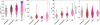 |
Fig. 11 Distribution of (left to right) the H2 volume density, gas kinetic temperature, dust temperature, and H2CO fractional abundance with evolutionary phases of our sample. The horizontal lines within the distribution marks the mean of our sub-sample, gray distributions in the H2 volume density and dust temperature shows the mean of the ATLASGAL sample by Urquhart et al. (2022), and blue distribution in the H2 volume density is the ATLASGAL Top 100 sample by Giannetti et al. (2025). |
6.3.3 Fractional abundance of H2CO
The right-most plot in Fig. 11 shows a constant H2CO fractional abundance of ∼10−10 across evolutionary phases, with mean values differing by less than a factor of two. This apparent uniformity, also noted by Tang et al. (2017), suggests that the formation and destruction of H2CO is not strongly influenced by the dynamical evolution of the star-forming environment. Given that H2CO can form through both gas-phase reactions (e.g., CH3 + O → H + H2CO) and grain-surface processes (e.g., H + HCO → H2CO Punanova et al. 2025; Potapov & Garrod 2024), the observed stability may reflect a balance between these formation pathways across different phases. Consequently, we affirm that H2CO is a reliable tracer of dense gas in various stages of star formation, largely due to its chemically resilient abundance profile.
7 Summary and conclusion
In this paper, we have determined the gas kinetic temperature, volume density, and column density of clumps in Cygnus-X, the GLOSTAR pilot region, and M8 using the pyradex+emcee approach. Our analysis encompasses four transitions of H2COobserved with the IRAM 30-m and APEX 12-m telescopes. The main results are summarized as follows:
We observed a high detection rate of the four transitions. Regarding H2CO (10,1 − 00,0) and H2CO (30,3− 20,2), they were detected in 100% of sources in Cygnus-X and the GLOSTAR pilot region. The weaker emission lines H2CO (32,2 − 22,1) and H2CO (32,1 − 22,0) have detection rates of greater than 80% in these two regions. In M8, H2CO (10,1 − 00,0) and H2CO (30,3 − 20,2) were detected in 94% of sources, while the detection rate for H2CO (32,2 − 22,1) was 48%, the lowest among the transitions. The consistently high detection rates of these low-energy H2CO lines highlight their effectiveness as widespread tracers of molecular gas in diverse environments.
The pyradex+emcee method, assuming non-LTE conditions succeeds in reproducing the intensities of H2CO transitions that probe the same gas. We examined 102 sources across the three source catalogs and successfully obtained the physical conditions.
We obtained volume densities of n(H2) = 5.4 104 −3.8 105 cm−3, gas kinetic temperatures of Tgas = 16−219 K, and H2CO column densities of N(H2CO) = 6.0 × 10¹² − 1.6 × 1015 cm−2 in the Cygnus-X region, GLOSTAR pilot region, and M8 region. The non-LTE and LTE gas kinetic temperatures agree well below the critical density of H2CO (30,3−20,2) (∼105.5 cm−3). Above this value, the LTE gas kinetic temperatures, obtained from the intensity ratios of I(30,3 − 20,2)/I(32,1 − 22,0), overestimate the modeled non-LTE gas kinetic temperatures. The volume densities that we measured in Cygnus-X and M8 using H2CO align well with those determined from the 1.2-mm continuum emission.
We determined the evolutionary phases of 90 clumps in the Cygnus-X and the M8 region. We find a significant order-of-magnitude increase in the H2 volume density across evolutionary phases, indicating dynamic processes in star-forming regions. This observed trend, predicted by theoretical models, suggests that gas accretion outpaces negative feedback, leading to denser clumps and more effective conditions for star formation. The dust temperature increases with evolutionary phases. We observed that the dust temperatures during the evolutionary phases consistently remain lower than the gas kinetic temperatures. Surprisingly, we find that the gas kinetic temperatures, obtained with pyradex+emcee, remain constant throughout the evolutionary phases. The H2CO may trace more diffuse gas despite its critical densities, suggesting it should exist in denser regions (e.g., the case for HCN; Kauffmann et al. 2017). The temperature discrepancy found between the dust and gas indicates that the gas and dust are decoupled.
The H2CO fractional abundance remains relatively constant at ∼10−10 across different evolutionary phases. This stable abundance throughout star formation affirms that H2CO can be effectively used to study gas in different phases and is consistent with findings from Tang et al. (2017).
The H2CO (10,1 − 00,0) line, newly accessible with the IRAM 30-m telescope, along with beam-matched data for the H2CO (30,3 20,2), H2CO (32,2 − 22,1), and H2CO (32,1 − 22,0) lines from APEX− 12-m allowed us to constrain a wide range of physical conditions in molecular clouds. The ground-state transition allowed us to probe the bulk of the gas volume densities. We identified an increasing trend of the H2 volume densities with evolving clumps. The CASCADE survey has performed equivalent observations of Cygnus-X with the NOEMA telescope, making it possible to expand this analysis to smaller core scales.
Data availability
The appendix Tables A.1, A.2, A.3, B.1, B.2, B.3, C.1, and D.1 are available at the CDS via https://cdsarc.cds.unistra.fr/viz-bin/cat/J/A+A/708/A201.
Acknowledgements
The authors would like to thank the anonymous referee for their suggestions and constructive comments that improved the overall quality of the manuscript. The authors are grateful to the staff at the Pico Veleta observatories and APEX for their support of these observations. I.B.C. is a fellow of the International Max-Planck-Research School (IMPRS) for A&A at the Universities of Bonn and Cologne. This work is based on observations carried out under project number 145-19, 031-20, 110-15, and 141-21 with the IRAM 30-m telescope. IRAM is supported by INSU/CNRS (France), MPG (Germany) and IGN (Spain). This publication is based on data acquired with the Atacama Pathfinder Experiment (APEX) under program ID M-0109.F9508C-2022, M-099.F9519A-2017, and M-0107.F9530C-2021. APEX has been a collaboration between the Max-Planck-Institut für Radioastronomie, the European Southern Observatory, and the Onsala Space Observatory. I.B.C. thanks A. Cheema for help with the determination of evolutionary phases in the M8 clumps. Y.G. was supported by the Ministry of Science and Technology of China under the National Key R&D Program (Grant No. 2023YFA1608200), the National Natural Science Foundation of China (Grant No. 12427901), and the Strategic Priority Research Program of the Chinese Academy of Sciences (Grant No. XDB0800301).
References
- Akabane, K., Morimoto, M., Nagane, K., et al. 1974, PASJ, 26, 1 [Google Scholar]
- Ao, Y., Henkel, C., Menten, K. M., et al. 2013, A&A, 550, A135 [NASA ADS] [CrossRef] [EDP Sciences] [Google Scholar]
- Arias, J. I., Barbá, R. H., Maíz Apellániz, J., Morrell, N. I., & Rubio, M. 2006, MNRAS, 366, 739 [NASA ADS] [CrossRef] [Google Scholar]
- Baars, J. W. M., Hooghoudt, B. G., Mezger, P. G., & de Jonge, M. J. 1987, A&A, 175, 319 [NASA ADS] [Google Scholar]
- Battersby, C., Walker, D. L., Barnes, A., et al. 2025, ApJ, 984, 156 [Google Scholar]
- Beerer, I. M., Koenig, X. P., Hora, J. L., et al. 2010, ApJ, 720, 679 [Google Scholar]
- Beuther, H., Gieser, C., Soler, J. D., et al. 2024, A&A, 682, A81 [NASA ADS] [CrossRef] [EDP Sciences] [Google Scholar]
- Beuther, H., Schilke, P., Menten, K. M., et al. 2002, ApJ, 566, 945 [Google Scholar]
- Beuther, H., Wyrowski, F., Menten, K. M., et al. 2022, A&A, 665, A63 [NASA ADS] [CrossRef] [EDP Sciences] [Google Scholar]
- Bonne, L., Bontemps, S., Schneider, N., et al. 2023, ApJ, 951, 39 [CrossRef] [Google Scholar]
- Brunthaler, A., Menten, K. M., Dzib, S. A., et al. 2021, A&A, 651, A85 [EDP Sciences] [Google Scholar]
- Cao, Y., Qiu, K., Zhang, Q., et al. 2019, ApJS, 241, 1 [Google Scholar]
- Carey, S. J., Noriega-Crespo, A., Mizuno, D. R., et al. 2009, PASP, 121, 76 [Google Scholar]
- Carter, M., Lazareff, B., Maier, D., et al. 2012, A&A, 538, A89 [NASA ADS] [CrossRef] [EDP Sciences] [Google Scholar]
- Chen, L., de Grijs, R., & Zhao, J. L. 2007, AJ, 134, 1368 [NASA ADS] [CrossRef] [Google Scholar]
- Churchwell, E., Babler, B. L., Meade, M. R., et al. 2009, PASP, 121, 213 [Google Scholar]
- Coletta, A., Molinari, S., Schisano, E., et al. 2025, A&A, 696, A151 [NASA ADS] [CrossRef] [EDP Sciences] [Google Scholar]
- Csengeri, T., Urquhart, J. S., Schuller, F., et al. 2014, A&A, 565, A75 [NASA ADS] [CrossRef] [EDP Sciences] [Google Scholar]
- Cummins, S. E., Green, S., Thaddeus, P., & Linke, R. A. 1983, ApJ, 266, 331 [NASA ADS] [CrossRef] [Google Scholar]
- Damiani, F., Bonito, R., Prisinzano, L., et al. 2017, A&A, 604, A135 [NASA ADS] [CrossRef] [EDP Sciences] [Google Scholar]
- Dislaire, V., Hily-Blant, P., Faure, A., et al. 2012, A&A, 537, A20 [NASA ADS] [CrossRef] [EDP Sciences] [Google Scholar]
- Dokara, R., Brunthaler, A., Menten, K. M., et al. 2021, A&A, 651, A86 [EDP Sciences] [Google Scholar]
- Dokara, R., Gong, Y., Reich, W., et al. 2023, A&A, 671, A145 [NASA ADS] [CrossRef] [EDP Sciences] [Google Scholar]
- Downes, D., Wilson, T. L., Bieging, J., & Wink, J. 1980, A&AS, 40, 379 [Google Scholar]
- Fixsen, D. J. 2009, ApJ, 707, 916 [Google Scholar]
- Gerin, M., Liszt, H., Pety, J., & Faure, A. 2024, A&A, 686, A49 [NASA ADS] [CrossRef] [EDP Sciences] [Google Scholar]
- Giannetti, A., Leurini, S., Wyrowski, F., et al. 2017, A&A, 603, A33 [NASA ADS] [CrossRef] [EDP Sciences] [Google Scholar]
- Giannetti, A., Leurini, S., Schisano, E., et al. 2025, A&A, 698, A90 [NASA ADS] [CrossRef] [EDP Sciences] [Google Scholar]
- Gieser, C., Beuther, H., Semenov, D., et al. 2021, A&A, 648, A66 [EDP Sciences] [Google Scholar]
- Gieser, C., Beuther, H., Semenov, D., et al. 2023, A&A, 674, A1605 [Google Scholar]
- Ginsburg, A., Bally, J., Battersby, C., et al. 2015, A&A, 573, A106 [NASA ADS] [CrossRef] [EDP Sciences] [Google Scholar]
- Ginsburg, A., Darling, J., Battersby, C., Zeiger, B., & Bally, J. 2011, ApJ, 736, 149 [NASA ADS] [CrossRef] [Google Scholar]
- Girichidis, P., Federrath, C., Banerjee, R., & Klessen, R. S. 2011, MNRAS, 413, 2741 [Google Scholar]
- Girichidis, P., Offner, S. S. R., Kritsuk, A. G., et al. 2020, Space Sci. Rev., 216, 68 [NASA ADS] [CrossRef] [Google Scholar]
- Goldsmith, P. F. 2001, ApJ, 557, 736 [Google Scholar]
- Gong, Y., Ortiz-León, G. N., Rugel, M. R., et al. 2023, A&A, 678, A130 [NASA ADS] [CrossRef] [EDP Sciences] [Google Scholar]
- Güsten, R., Nyman, L. Å., Schilke, P., et al. 2006, A&A, 454, L13 [NASA ADS] [CrossRef] [EDP Sciences] [Google Scholar]
- Guzmán, V. V., Goicoechea, J. R., Pety, J., et al. 2013, A&A, 560, A73 [Google Scholar]
- Hennemann, M., Motte, F., Schneider, N., et al. 2012, A&A, 543, L3 [NASA ADS] [CrossRef] [EDP Sciences] [Google Scholar]
- Henshaw, J. D., Barnes, A. T., Battersby, C., et al. 2023, ASP Conf. Ser., 534, 83 [NASA ADS] [Google Scholar]
- Holland, W. S., Robson, E. I., Gear, W. K., et al. 1999, MNRAS, 303, 659 [NASA ADS] [CrossRef] [Google Scholar]
- Kahle, K. A., Wyrowski, F., König, C., et al. 2024, A&A, 687, A162 [NASA ADS] [CrossRef] [EDP Sciences] [Google Scholar]
- Kaifu, N., Iguchi, T., & Morimoto, M. 1975, ApJ, 196, 719 [Google Scholar]
- Kauffmann, J., Goldsmith, P. F., Melnick, G., et al. 2017, A&A, 605, L5 [NASA ADS] [CrossRef] [EDP Sciences] [Google Scholar]
- Kim, W. J., Beuther, H., Wyrowski, F., et al. 2025, A&A, 694, A30 [NASA ADS] [CrossRef] [EDP Sciences] [Google Scholar]
- Knödlseder, J. 2000, A&A, 360, 539 [NASA ADS] [Google Scholar]
- König, C., Urquhart, J. S., Csengeri, T., et al. 2017, A&A, 599, A139 [Google Scholar]
- Kraemer, K. E., Hora, J. L., Egan, M. P., et al. 2010, AJ, 139, 2319 [Google Scholar]
- Krumholz, M. R., & Bonnell, I. A. 2009, in Structure Formation in Astrophysics, ed. G. Chabrier (Cambridge: Cambridge University Press), 288 [Google Scholar]
- Leurini, S., Schilke, P., Menten, K. M., et al. 2004, A&A, 422, 573 [NASA ADS] [CrossRef] [EDP Sciences] [Google Scholar]
- Leurini, S., Schilke, P., Wyrowski, F., & Menten, K. M. 2007, A&A, 466, 215 [NASA ADS] [CrossRef] [EDP Sciences] [Google Scholar]
- Lin, Y., Wyrowski, F., Liu, H. B., et al. 2022, A&A, 658, A128 [NASA ADS] [CrossRef] [EDP Sciences] [Google Scholar]
- Mangum, J. G., & Wootten, A. 1993, ApJS, 89, 123 [Google Scholar]
- Mangum, J. G., Wootten, A., Loren, R. B., & Wadiak, E. J. 1990, ApJ, 348, 542 Mangum, J. G., Darling, J., Menten, K. M., & Henkel, C. 2008, ApJ, 673, 832 [Google Scholar]
- Mangum, J. G., Darling, J., Henkel, C., & Menten, K. M. 2013, ApJ, 766, 108 [NASA ADS] [CrossRef] [Google Scholar]
- Marsh, K. A., Ragan, S. E., Whitworth, A. P., & Clark, P. C. 2016, MNRAS, 461, L16 [Google Scholar]
- McKee, C. F., & Ostriker, E. C. 2007, ARA&A, 45, 565 [Google Scholar]
- McKee, C. F., & Tan, J. C. 2002, Nature, 416, 59 [CrossRef] [Google Scholar]
- Medina, S. N. X., Urquhart, J. S., Dzib, S. A., et al. 2019, A&A, 627, A175 [NASA ADS] [CrossRef] [EDP Sciences] [Google Scholar]
- Molinari, S., Brand, J., Cesaroni, R., Palla, F., & Palumbo, G. G. C. 1998, A&A, 336, 339 [NASA ADS] [Google Scholar]
- Mookerjea, B., Hassel, G. E., Gerin, M., et al. 2012, A&A, 546, A75 [NASA ADS] [CrossRef] [EDP Sciences] [Google Scholar]
- Motte, F., Bontemps, S., Schilke, P., et al. 2007, A&A, 476, 1243 [NASA ADS] [CrossRef] [EDP Sciences] [Google Scholar]
- Motte, F., Zavagno, A., Bontemps, S., et al. 2010, A&A, 518, L77 [CrossRef] [EDP Sciences] [Google Scholar]
- Müller, H. S. P., Thorwirth, S., Roth, D. A., & Winnewisser, G. 2001, A&A, 370, L49 [Google Scholar]
- Nguyen, H., Rugel, M. R., Murugeshan, C., et al. 2022, A&A, 666, A59 [NASA ADS] [CrossRef] [EDP Sciences] [Google Scholar]
- Offner, S. S. R., Taylor, J., Markey, C., et al. 2022, MNRAS, 517, 885 [NASA ADS] [CrossRef] [Google Scholar]
- Okoh, D., Esimbek, J., Zhou, J. J., et al. 2014, Ap & SS, 350, 657 [Google Scholar]
- Pagani, L., Vastel, C., Hugo, E., et al. 2009, A&A, 494, 623 [NASA ADS] [CrossRef] [EDP Sciences] [Google Scholar]
- Pandian, J. D., Chatterjee, R., Csengeri, T., et al. 2024, ApJ, 966, 54 [Google Scholar]
- Parmentier, G. 2020, ApJ, 893, 32 [Google Scholar]
- Perley, R. A., Chandler, C. J., Butler, B. J., & Wrobel, J. M. 2011, ApJ, 739, L1 [Google Scholar]
- Pety, J. 2018, in Submillimetre Single-dish Data Reduction and Array Combination Techniques, 11 [Google Scholar]
- Pillai, T., Kauffmann, J., Wyrowski, F., et al. 2011, A&A, 530, A118 [CrossRef] [EDP Sciences] [Google Scholar]
- Pokhrel, R., Myers, P. C., Dunham, M. M., et al. 2018, ApJ, 853, 5 [NASA ADS] [CrossRef] [Google Scholar]
- Potapov, A., & Garrod, R. T. 2024, A&A, 692, A252 [NASA ADS] [CrossRef] [EDP Sciences] [Google Scholar]
- Punanova, A. F., Borshcheva, K., Fedoseev, G. S., et al. 2025, MNRAS, 537, 3686 [Google Scholar]
- Redaelli, E., Bizzocchi, L., Caselli, P., & Pineda, J. E. 2023, A&A, 674, L8 [NASA ADS] [CrossRef] [EDP Sciences] [Google Scholar]
- Reid, M. J., Menten, K. M., Brunthaler, A., et al. 2019, ApJ, 885, 131 [Google Scholar]
- Remijan, A., Sutton, E. C., Snyder, L. E., et al. 2004, ApJ, 606, 917 [NASA ADS] [CrossRef] [Google Scholar]
- Roman-Duval, J., Jackson, J. M., Heyer, M., et al. 2009, ApJ, 699, 1153 [CrossRef] [Google Scholar]
- Rygl, K. L. J., Brunthaler, A., Sanna, A., et al. 2012, A&A, 539, A79 [NASA ADS] [CrossRef] [EDP Sciences] [Google Scholar]
- Schneider, N., Csengeri, T., Bontemps, S., et al. 2010, A&A, 520, A49 [CrossRef] [EDP Sciences] [Google Scholar]
- Schneider, N., Bonne, L., Bontemps, S., et al. 2023, Nat. Astron., 7, 546 [NASA ADS] [CrossRef] [Google Scholar]
- Schuller, F., Menten, K. M., Contreras, Y., et al. 2009, A&A, 504, 415 [NASA ADS] [CrossRef] [EDP Sciences] [Google Scholar]
- Shirley, Y. L. 2015, PASP, 127, 299 [Google Scholar]
- Shu, F. H., Adams, F. C., & Lizano, S. 1987, ARA&A, 25, 23 [CrossRef] [Google Scholar]
- Tafalla, M., Myers, P. C., Caselli, P., & Walmsley, C. M. 2004, A&A, 416, 191 [NASA ADS] [CrossRef] [EDP Sciences] [Google Scholar]
- Tan, J. C., Krumholz, M. R., & McKee, C. F. 2006, ApJ, 641, L121 [CrossRef] [Google Scholar]
- Tang, X. D., Henkel, C., Chen, C. H. R., et al. 2017, A&A, 600, A16 [NASA ADS] [CrossRef] [EDP Sciences] [Google Scholar]
- Tang, X. D., Henkel, C., Wyrowski, F., et al. 2018, A&A, 611, A6 [NASA ADS] [CrossRef] [EDP Sciences] [Google Scholar]
- Tang, X. D., Henkel, C., Menten, K. M., et al. 2021a, A&A, 655, A12 [NASA ADS] [CrossRef] [EDP Sciences] [Google Scholar]
- Tang, Y., Wang, Q. D., & Wilson, G. W. 2021b, MNRAS, 505, 2377 [NASA ADS] [CrossRef] [Google Scholar]
- Tielens, A. 2021, Molecular Astrophysics (Cambridge: Cambridge University Press) [Google Scholar]
- Tiwari, M., Menten, K. M., Wyrowski, F., et al. 2019, A&A, 626, A28 [NASA ADS] [CrossRef] [EDP Sciences] [Google Scholar]
- Tiwari, M., Menten, K. M., Wyrowski, F., et al. 2020, A&A, 644, A25 [NASA ADS] [CrossRef] [EDP Sciences] [Google Scholar]
- Tothill, N. F. H., White, G. J., Matthews, H. E., et al. 2002, ApJ, 580, 285 [Google Scholar]
- Tothill, N. F. H., Gagné, M., Stecklum, B., & Kenworthy, M. A. 2008, ASP Conf. Ser., 5, 533 [Google Scholar]
- Urquhart, J. S., König, C., Giannetti, A., et al. 2018, MNRAS, 473, 1059 [Google Scholar]
- Urquhart, J. S., Wells, M. R. A., Pillai, T., et al. 2022, MNRAS, 510, 3389 [NASA ADS] [CrossRef] [Google Scholar]
- van der Tak, F. F. S., Black, J. H., Schöier, F. L., Jansen, D. J., & van Dishoeck, E. F. 2007, A&A, 468, 627 [NASA ADS] [CrossRef] [EDP Sciences] [Google Scholar]
- Vázquez-Semadeni, E., Palau, A., Ballesteros-Paredes, J., Gómez, G. C., & Zamora-Avilés, M. 2019, MNRAS, 490, 3061 [Google Scholar]
- Vázquez-Semadeni, E., Gómez, G. C., & González-Samaniego, A. 2024, MNRAS, 530, 3445 [CrossRef] [Google Scholar]
- Walmsley, C. M., & Ungerechts, H. 1983, A&A, 122, 164 [Google Scholar]
- Watanabe, N., & Kouchi, A. 2002, ApJ, 571, L173 [Google Scholar]
- Wienen, M., Wyrowski, F., Schuller, F., et al. 2012, A&A, 544, A146 [NASA ADS] [CrossRef] [EDP Sciences] [Google Scholar]
- Wiesenfeld, L., & Faure, A. 2013, MNRAS, 432, 2573 [NASA ADS] [CrossRef] [Google Scholar]
- Woon, D. E. 2002, ApJ, 569, 541 [Google Scholar]
- Wright, N. J., Drew, J. E., & Mohr-Smith, M. 2015, MNRAS, 449, 741 [NASA ADS] [CrossRef] [Google Scholar]
- Yamato, Y., Furuya, K., Aikawa, Y., et al. 2022, ApJ, 941, 75 [NASA ADS] [CrossRef] [Google Scholar]
- Yan, Y. T., Zhang, J. S., Henkel, C., et al. 2019, ApJ, 877, 154 [Google Scholar]
- Yang, C., Omont, A., Beelen, A., et al. 2017, A&A, 608, A144 [NASA ADS] [CrossRef] [EDP Sciences] [Google Scholar]
- Zhang, B., Moscadelli, L., Sato, M., et al. 2014, ApJ, 781, 89 [Google Scholar]
The 100-m telescope at Effelsberg is operated by the Max-Planck Institut für Radioastronomie (MPIfR) on behalf of the Max-Planck Gesellschaft (MPG).
The beam efficiency for the M8 sources is adopted from the publicly available line monitoring of APEX telescope receivers https://www.apex-telescope.org/telescope/efficiency/
Appendix A Clumps locations in Cygnus-X, the GLOSTAR pilot region, and M8
The pointing coordinates of clumps in Cygnus-X, the GLOSTAR pilot region, and M8 are given in Tables A.1, A.2, and A.3, respectively.
Clump positions in Cygnus-X.
Clump positions in the GLOSTAR pilot region.
Clump positions observed with the APEX 12-m and the IRAM 30-m telescopes. Sources marked with a * have been observed at deviating positions with the IRAM 30 meter telescope (M8WC3: 18h03m44.8s, −24°21′03′′, M8SE8: 18h04m50.5s, −24°27′33′′, M8SC5: 18h03m40.7s, −24°26′59′′) to properly match the dust continuum peaks.
Overview of the reference positions and the number of clumps in the regions of Cygnus-X, including the number of clumps.
Appendix B Line profile measurements of H2CO
The obtained integrated intensities and linewidths of H2CO (10,1 − 00,0), H2CO (30,3 − 20,2), H2CO (32,2 − 22,1), and H2CO (32,1 − 22,0) in Cygnus-X are presented in Table B.1. Similarly, Table B.2 presented the sources in the GLOSTAR pilot region, and Table B.3 presents the sources in the M8 region.
The integrated intensities and mean linewidth of the four H2CO transitions.
GLOSTAR integrated intensities and mean linewidth of the four H2CO transitions.
M8 integrated intensities and linewidth of the four mean H2CO transitions.
Number of discarded source with each criteria.
Appendix C pyradex+emcee results
The obtained values of volume density, gas kinetic temperature, and H2CO column densities for clumps in all regions are presented in Table C.1.
Volume density, gas kinetic temperature, H2CO column density, and number of lines used during modeling for all sources.
Appendix D The evolutionary phases of clumps
The detection of emission in continuum, 70 µm, 24 µm, and 3.6 µm, and their determined evolutionary phase of clumps in Cygnus-X and M8.
All Tables
Clump positions observed with the APEX 12-m and the IRAM 30-m telescopes. Sources marked with a * have been observed at deviating positions with the IRAM 30 meter telescope (M8WC3: 18h03m44.8s, −24°21′03′′, M8SE8: 18h04m50.5s, −24°27′33′′, M8SC5: 18h03m40.7s, −24°26′59′′) to properly match the dust continuum peaks.
Overview of the reference positions and the number of clumps in the regions of Cygnus-X, including the number of clumps.
GLOSTAR integrated intensities and mean linewidth of the four H2CO transitions.
Volume density, gas kinetic temperature, H2CO column density, and number of lines used during modeling for all sources.
The detection of emission in continuum, 70 µm, 24 µm, and 3.6 µm, and their determined evolutionary phase of clumps in Cygnus-X and M8.
All Figures
|
Fig. 1 Line-ratios of H2CO (30,3 − 20,2)/(10,1 − 00,0) (top) and H2CO (32,1 − 22,0)/(30,3 − 20,2) as a function of volume densities and gas kinetic temperature computed from pyradex. Bottom plot shows the “bump” at n(H2) ≥ 105.5 cm−3, discussed in Sect 6.1. |
| In the text | |
|
Fig. 2 Locations of clumps in Cygnus-X (top), the GLOSTAR pilot region (bottom left), and M8 (bottom right). |
| In the text | |
|
Fig. 3 Spectra of the four H2CO transitions toward six clumps, two from each region. The background color indicates whether a line is at ≥4σ (green) or <4σ (red). The dashed black line indicates the peak velocity of the fit Gaussian for each transition. Examples of clumps with too few lines (N33), differences in ∆υ (N46), or a double peak (G28.28–0.36) are shown. |
| In the text | |
|
Fig. 4 Top row: difference in υpeak between the H2CO (10,1 − 00,0) line and the three higher J-transitions of H2CO. The X (in the y-axis) denotes the υpeak noted in the x-axis. Bottom row: linewidths of the different H2CO transitions. In top and bottom rows, sources in Cygnus-X are shown in purple, GLOSTAR sources in orange, and M8 sources in blue. The black symbols indicate clumps that do not satisfy the velocity criterion (green shaded region) and were excluded from further analysis. |
| In the text | |
|
Fig. 5 Comparison of H2CO (32,2 − 22,1) and H2CO (32,1 − 22,0) integrated intensities. The sources in Cygnus-X, the GLOSTAR pilot region, and M8 are shown in purple, orange, and blue, respectively. |
| In the text | |
|
Fig. 6 Distribution of (left to right) the H2 volume density, gas kinetic temperature, the H2CO column density, and the fractional abundance. The sources in Cygnus-X, the GLOSTAR pilot region, and M8 are shown in purple, orange, and blue across all distributions, respectively. Similar high-mass sources from the ATLASGAL Top 100, measured using higher J-transitions of H2CO by Tang et al. (2018) are depicted in gray. |
| In the text | |
|
Fig. 7 Gas kinetic temperature of sources in Cygnus-X (purple), the GLOSTAR pilot region (orange), and M8 (blue) using pyradex+emcee. The gray points show the temperatures obtained for the ATLASGAL sources by Tang et al. (2018). The dashed red line shows the LTE gas kinetic temperature function presented in Eq. (4). |
| In the text | |
|
Fig. 8 Difference between the gas kinetic temperature of sources in Cygnus-X (purple), the GLOSTAR pilot region (orange), and M8 (blue) using pyradex+emcee compared with the LTE gas kinetic temperature function presented in Tang et al. (2018). The dashed green line marks n(H2) = 105.5 cm−3. |
| In the text | |
|
Fig. 9 Comparison of volume densities in Cygnus-X (purple) and M8 (blue) obtained with pyradex+emcee and the 1.2-mm continuum emission by Motte et al. (2007) for Cygnus-X and Tothill et al. (2002) for M8. The dashed gray line shows x = y. |
| In the text | |
|
Fig. 10 Distribution of the evolutionary phases of the clumps in the Cygnus-X (left) and M8 region (right). “Protost”. denotes protostellar and “Quiesc”. denotes quiescent stage. |
| In the text | |
|
Fig. 11 Distribution of (left to right) the H2 volume density, gas kinetic temperature, dust temperature, and H2CO fractional abundance with evolutionary phases of our sample. The horizontal lines within the distribution marks the mean of our sub-sample, gray distributions in the H2 volume density and dust temperature shows the mean of the ATLASGAL sample by Urquhart et al. (2022), and blue distribution in the H2 volume density is the ATLASGAL Top 100 sample by Giannetti et al. (2025). |
| In the text | |
Current usage metrics show cumulative count of Article Views (full-text article views including HTML views, PDF and ePub downloads, according to the available data) and Abstracts Views on Vision4Press platform.
Data correspond to usage on the plateform after 2015. The current usage metrics is available 48-96 hours after online publication and is updated daily on week days.
Initial download of the metrics may take a while.