| Issue |
A&A
Volume 708, April 2026
|
|
|---|---|---|
| Article Number | A134 | |
| Number of page(s) | 18 | |
| Section | Planets, planetary systems, and small bodies | |
| DOI | https://doi.org/10.1051/0004-6361/202558201 | |
| Published online | 01 April 2026 | |
Spectrophotometric properties of Martian soil at the landing area of the Tianwen–1 Zhurong rover
1
State Key Laboratory of Solar Activity and Space Weather, National Space Science Center, Chinese Academy of Sciences,
Beijing,
China
2
College of Earth and Planetary Sciences, University of Chinese Academy of Sciences,
Beijing,
China
3
Aix Marseille Univ, CNRS, CNES, LAM,
Marseille,
France
4
State Key Laboratory of Remote Sensing and Digital Earth, Aerospace Information Research Institute, Chinese Academy of Sciences,
Beijing
100101,
China
5
Key Laboratory of Lunar and Deep Space Exploration, National Astronomical Observatories, Chinese Academy of Sciences,
Beijing,
China
6
Key Laboratory of Planetary Science and Frontier Technology, Chinese Academy of Sciences,
Beijing
100029,
China
★ Corresponding author: This email address is being protected from spambots. You need JavaScript enabled to view it.
Received:
21
November
2025
Accepted:
11
February
2026
Abstract
Context. The Navigation and Terrain Camera (NaTeCam) on board the Zhurong rover acquired extensive imaging data of the landing site under a wide range of phase angles, providing a unique opportunity to investigate the photometric properties of this area.
Aims. We aim to retrieve the photometric and microphysical properties of the widely distributed soil units in the landing area, assess their implications for surface scattering behavior, and provide new ground-truth photometric constraints for this region.
Methods. We extracted phase curves from five Martian-day datasets, corrected them for diffuse skylight using the DISORT (DIScrete Ordinates Radiative Transfer) radiative transfer model, and inverted the photometric parameters by coupling the Hapke radiative transfer model with a parallel Monte Carlo approach.
Results. The soils exhibit backscattering-dominated behavior, relatively high particle porosity and/or heterogeneous size distributions, and low macroscopic roughness. The phase reddening effect is also observed, with a maximum near 60°.
Conclusions. These photometric properties provide key ground-truth constraints for surface scattering models and enable more reliable quantitative spectral analyses of the Zhurong landing site and adjacent regions.
Key words: radiative transfer / techniques: photometric / planets and satellites: surfaces
© The Authors 2026
 Open Access article, published by EDP Sciences, under the terms of the Creative Commons Attribution License (https://creativecommons.org/licenses/by/4.0), which permits unrestricted use, distribution, and reproduction in any medium, provided the original work is properly cited.
This article is published in open access under the Subscribe to Open model. This email address is being protected from spambots. You need JavaScript enabled to view it. to support open access publication.
1 Introduction
The reflectance spectra of the Martian surface are determined not only by composition but also by illumination and viewing geometry. As a non-Lambertian surface, it usually exhibits anisotropic scattering, with reflected light intensity depending on emission direction, phase angle, and other factors. Moreover, the magnitude of variation differs among wavelengths at different phase angles, and the “phase reddening” phenomenon may occur (Guinness 1981; Johnson et al. 2015, 2021, 2022; Liang et al. 2020). This anisotropy is controlled by both mineralogy and micro-textural properties (i.e., particle size distribution, porosity, and surface roughness). By applying photometric models to data collected under varying illumination and viewing geometries, the parameters that quantitatively characterize the surface scattering properties can be retrieved. These photometric parameters provide improved constrains on the composition, mineralogy, and weathering histories of Martian surface (Johnson et al. 2008). They also enable more accurate characterization of Martian surface scattering behaviors, supporting quantitative spectral analysis (Audouard et al. 2014; Milliken et al. 2007; Liu et al. 2016; Zhou et al. 2023), and providing refined surface boundary conditions for climate models and atmospheric scattering studies (Moores et al. 2015; Vincendon et al. 2007; Wolff et al. 2009).
To obtain realistic photometric parameter information of the Martian surface, extensive photometric studies have been conducted on data from past Mars exploration missions. During early missions, such as Viking and Pathfinder, photometric investigations were focused on characterizing surface materials and atmospheric dust (Arvidson et al. 1989a,b; Bell et al. 2000; Guinness et al. 1997; Johnson et al. 1999; Pollack et al. 1995). Unlike other airless bodies, observations of the Martian surface are influenced by diffuse skylight scattered by the atmosphere (Thomas 2001; Tomasko et al. 1999; Lemmon et al. 2004). However, early studies, constrained by observational data and technical limitations, did not account for the contribution of this atmospheric diffuse component. Subsequent advancements in Martian atmospheric correction models refined in situ photometric analysis of soils, rocks, and other surface materials along the traverse paths of the Mars Exploration Rovers (MERs) and Curiosity (Johnson et al. 2006a,b, 2015, 2021, 2022; Liang et al. 2020). These studies provided valuable ground-truth photometric parameters for the explored sites and investigated the phase reddening phenomenon, showing that the scattering properties of the Martian surface at the rover scale are strongly influenced by both local environmental conditions and the surrounding geological and topographical context. However, the spatial coverage of in situ photometric measurements remains extremely limited, with ground-truth information available for only a few landing sites. Consequently, some previous quantitative analyses have had to rely on the simple assumption of Lambertian surfaces or adopt photometric properties from MERs or Curiosity (Wolff et al. 2009; Liu et al. 2016; Zhou et al. 2023), which may introduce certain uncertainties.
To extend photometric investigations to a large scale, orbital instruments such as OMEGA and CRISM have been utilized. Using these datasets, Vincendon (2013) derived Mars’ globally averaged photometric parameters. Subsequent analyses on multi-angle CRISM observations of overlapping regions quantified grain-scale surface properties, demonstrating the potential of photometric parameters in constraining local geological processes (Fernando et al. 2013, 2015, 2016; Shaw et al. 2013). However, orbital observations are constrained by limited viewing geometries, and individual datasets typically provide only narrow phase angle coverage. Moreover, observations acquired at different times are affected by varying atmospheric conditions, and the photometric parameters derived from orbital modeling still require validation against ground-truth measurements.
In parallel, laboratory photometric experiments on planetary surface analogs have revealed photometric parameter variations across different materials (Johnson et al. 2013; McGuire & Hapke 1995; Pilorget et al. 2016; Pommerol et al. 2013; Sun et al. 2023), thereby providing essential references for planetary surface photometry. Collectively, these efforts have laid the foundation for light-scattering modeling of planetary surfaces.
China’s Tianwen-1 mission successfully deployed the Zhurong rover to the southern Utopia Planitia region of Mars (Liu et al. 2022a). The landing site is located within a geologically young, mid-Amazonian unit, characterized by numerous geomorphological features that are likely associated with volatile-related or ice-related processes, such as pitted cones and giant polygons (Wu et al. 2021). Recent studies based on Zhurong mission data further suggest the possible presence of minor aqueous activities and evidence of recent glacial or periglacial evolution in this region (Liu et al. 2022b, 2023b; Qin et al. 2023). Compared with the landing sites of the MERs and Curiosity, the Zhurong site exhibits higher dust coverage (Ruff & Christensen 2002), indicating that its surface is more strongly influenced by dust mantling. Therefore, apart from its regional importance, the photometric characteristics of this area could be more representative of dust-dominated surfaces elsewhere on Mars.
During its traverse, the rover’s Navigation and Terrain Cameras (NaTeCam) acquired a large volume of image data, including multiphase angle observations from 360° panoramic imaging conducted over several Martian days (Sols). These datasets cover a broad range of phase angles within a short time interval, which ensures minimal variations in illumination and atmospheric conditions and provides a robust basis for reliably investigating the photometric properties of this previously unexplored Martian region. In this study, we conducted a photometric analysis of the widespread soils at the landing site. Phase curves were extracted and corrected for diffuse skylight, and photometric parameters were retrieved via a parallel Monte Carlo inversion, providing new ground-truth constraints on Martian surface scattering properties. The paper is structured as follows: Section 2 introduces the data and methodology, Section 3 presents the results, Section 4 provides a discussion, and the final section summarizes the study.
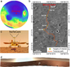 |
Fig. 1 Location of the Zhurong landing site and NaTeCam datasets. (a) Location of the Zhurong landing site, overlaid on a MOLA digital terrain model. (b) Traverse path of Zhurong and locations of the acquired panoramic NaTeCam datasets, overlaid on a Tianwen-1 High-Resolution Imaging Camera (HiRIC) image (HX1_GRAS_HIRIC_DIM_0.7_0004_251515N1095850E_A). (c) Zhurong rover selfie and the position of NaTeCam on the rover; the selfie was taken by a small detachable camera carried by the rover. (d) 360° panoramic image acquired by NaTeCam on Sol 32. |
2 Data and methods
2.1 Data
During the Zhurong rover’s traverse, the onboard Navigation and Terrain Cameras (NaTeCam) acquired a large volume of surface images around the landing site. NaTeCam consists of a stereo pair of left and right cameras. The raw data underwent standard processing, including bias and dark current removal, flat-field correction, and radiometric calibration to produce Level 2B radiance data (2048 × 2048 pixels per image).
Equipped with a Bayer filter (GBRG mode), NaTeCam initially provides single-band Level 2B data, which can be converted into three-band RGB images with central wavelengths of 650 nm (R), 550 nm (G), and 480 nm (B). More details on the instrument design and data processing of NaTeCam can be found in Liang et al. (2021). In this study, we focus on photometric analysis of the RGB-converted Level 2B radiance data acquired during Zhurong’s 2 km traverse over 325 Sols. The landing site predominantly consists of soils, dunes, rocks, and duricrust, with soils being the most widespread (Liu et al. 2022b). For representative photometric characterization, we analyzed soil units using data from Sols 05, 32, 58, 84, and 99, which were selected for 360° panoramic imaging over short time intervals under consistent illumination and atmospheric conditions. Each panoramic dataset comprises 12 stereo pairs (left and right cameras), with corresponding observation locations shown in Fig. 1b. Notably, Sol 05 dataset was acquired close to the lander, where the surface soils had been blown away by the lander’s descent plume, while Sol 99 dataset was collected near a Transverse Aeolian Ridges (TAR). The phase angle coverage and relevant parameters for the five datasets are summarized in Table 1.
Information of datasets used in this study.
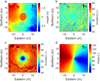 |
Fig. 2 Photometry QUBs of the study area (Sol 32). The X-axis increases eastward, and the Y-axis increases northward, with the origin at the NaTeC am camera position. (a) Relative elevation with respect to NaTeCam. (b) Incidence angle. (c) Emission angle. (d) Phase angle. |
2.2 Phase curve extraction
Using NaTeCam’s panoramic stereo images, we generated a Digital Orthophoto Map (DOM) and constructed a Digital Elevation Model (DEM; Fig. 2a) at a spatial resolution of 2 cm per pixel, from which pixel-level XYZ coordinates were derived. Based on the DEM, the surface normal vector (UVW) of each pixel was calculated, combined with the solar azimuth and elevation angles and camera position data to determine incident and emission light vectors. This enabled computation of local incidence, emission, and phase angles (IEP) for each pixel (Figs. 2b–d). The combination of XYZ, UVW, and IEP values for each pixel constitutes the so-called Photometry QUBs(Johnson et al. 2006a,b; Soderblom et al. 2004).
Based on the DOM images (2 cm per pixel) and the corresponding phase angle distribution maps, soil units were selected from different phase angle ranges to extract the phase curves. Consistent with definitions adopted in previous studies (Johnson et al. 2006a,b, 2015; Liang et al. 2020; Johnson et al. 2021, 2022), the soil units in this work refer to relatively smooth surface areas that lack obvious coarse-grains and pebbles. Accordingly, during the selection of regions of interest (ROIs), we preferentially targeted areas dominated by fine-grained materials below the image resolution and avoided regions containing obvious coarse grains or pebbles. Shadowed areas (incidence angle >90°), non-observable regions (emission angle >90°) and pixels corresponding to obvious small pebbles were excluded from ROIs in the subsequent processing. For each ROI, the average value with associated uncertainty was calculated to generate phase curves for subsequent photometric fitting. Fig. 3 presents the DOM of sol 32 together with its corresponding phase curve, with the white box indicating the selected ROI. A distinct fan-shaped bright area is observed in the western direction of Fig. 3a (as shown by the red dashed line enclosed area), caused by rover coating reflections. Consequently, all ROI definitions excluded regions within ±30° of the solar azimuth to avoid rover-induced reflection contamination. Furthermore, this exclusion aligns with the Hapke model’s limitation in accounting for specular reflection effects (Hapke 1993; Johnson et al. 2006a), thereby reducing potential model-related uncertainties. The ROI selections, additional details, and the corresponding extracted phase curves for the other Sols are provided in Figs. B.1–B.5.
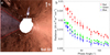 |
Fig. 3 DOMs and extracted phase curves of Sol 32. (a) DOMs for Sols 32. The white dashed lines indicate the boundaries of the mosaicking, and the white boxes mark the selected ROIs. The red dashed line encloses the area affected by reflections from the rover’s coating. (b) The corresponding phase curves extracted from the ROIs. |
2.3 Atmospheric correction
The Mars surface reflectance measurement is more complex than that of airless bodies due to atmospheric scattering contributions. Following Johnson et al. (2006a), we incorporated diffuse skylight modeling in our radiative transfer framework and subsequently removed its influence. The NaTeCam-observed radiance (Iobserved) can be modeled as:
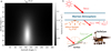 |
Fig. 4 Sky brightness model and schematic of the radiative transfer process. (a) Sky brightness model Isky(θ, ϕ) generated by DISORT (Sol 32, R band). (b) Schematic of the radiative transfer at the Martian surface. The radiance received by NaTeCam consists of both direct solar light and diffuse skylight. |
![Mathematical equation: $\[\begin{aligned}I_{\text {observed}}= & J_{\text {direct}} \cdot \exp \left(-\frac{\tau}{\mu_{\text {solar}}}\right) \cdot R_{\mathrm{bd}}(i, e, g) \\& +\int R_{\mathrm{bd}}(i^{\prime}, e, g^{\prime}) \cdot I_{\mathrm{sky}}(\theta, \phi) d \Omega.\end{aligned}\]$](/articles/aa/full_html/2026/04/aa58201-25/aa58201-25-eq1.png) (1)
(1)
The first term on the right-hand side of Eq. (1) represents the contribution from the direct solar illumination. Jdirect is the solar irradiance at the top of the atmosphere, adjusted for the corresponding Sun–Mars distance on the observation date. By convolving the solar spectrum with the NaTeCam’s spectral response functions (Liang et al. 2021), we derived bandspecific Jdirect values for the R, G, and B bands. The term τ denotes the atmospheric optical depth, and μsolar is the cosine of the solar incidence angle (note that this differs from the local incidence angle defined on inclined surfaces). Rbd is the bidirectional reflectance of the surface, defined as the ratio of observed radiance to incident irradiance. It is related to the radiance factor (RADF) by Rbd = RADF/π. Rbd was modeled using the Hapke photometric model for surface reflectance modeling (see Section 2.4). The local incidence (i), emission (e), and phase (g) angles are obtained from the Photometry QUBs framework described in Section 2.2.
The second term on the right-hand side of Eq. (1) represents the diffuse skylight component. Isky(θ, ϕ) is the sky radiance distribution function, describing the angular distribution of diffuse skylight. Here, i′ and g′ represent the effective incidence and phase angles associated with diffuse skylight reaching the surface from different directions. Isky (θ, ϕ) was modeled using the DISORT radiative transfer model (Stamnes et al. 1988; Liu & Wu 2023) by assuming a simplified plane-parallel, single-layer Martian atmosphere. The scattering properties of the atmosphere were adopted from Ockert-Bell et al. (1997). Because Zhurong lacks direct measurements of atmospheric optical depth (τ), the exact value of τ at the time of each NaTeCam acquisition cannot be directly determined. We therefore adopted a representative value of τ = 0.5, based on the indirectly retrieved optical depths reported by Zhang et al. (2023) for nearby sols. Zhang et al. (2023) showed that the optical depth over the first 110 sols at the landing site remained relatively stable, suggesting only limited temporal variability. To further assess the sensitivity of our results to this assumption, we performed additional tests by varying τ within ±0.05 of 0.5. The variations in the inversion results are almost entirely within, or very close to, the final uncertainty ranges reported in this study. Therefore, adopting τ = 0.5 is unlikely to significantly affect the sky radiance modeling or the photometric inversion, and this value was used in our analysis. Fig. 4a shows the DISORT-simulated R-band sky radiance for Sol 32, and Fig. 4b is a schematic diagram depicting the radiative transfer process described in Eq. (1).
For each ROI, we simulated combined direct and diffuse radiance under the corresponding illumination conditions. Following the method described in Johnson et al. (2006a), an initial guess of each photometric parameter was used to compute the corrected RADF. These photometric parameters were then refined through iterative fitting. After several iterations (typically converging in three iterations), we obtained the RADF corrected for diffuse skylight, which was then used to invert the photometric parameters.
2.4 Surface reflection model
To model the bidirectional reflectance (Rbd) of the landing site surface, we employ the Hapke scattering model, a classical framework for describing radiative transfer processes on planetary surfaces and has been widely applied in planetary spectral studies (Hapke 1993). The model’s bidirectional reflectance Rbd can be expressed as:
![Mathematical equation: $\[\begin{aligned}R_{\mathrm{bd}}(i, e, g)= & \frac{\omega}{4 \pi} \cdot \frac{\mu_0}{\mu_0+\mu} \cdot\left\{\left[1+B\left(g, h, B_0\right)\right] p(g)\right. \\& \left.+H\left(\mu_0\right) H(\mu)-1\right\} \cdot S(i, e, g, \theta),\end{aligned}\]$](/articles/aa/full_html/2026/04/aa58201-25/aa58201-25-eq2.png) (2)
(2)
where ω denotes the single scattering albedo (SSA); i, e, and g are the incidence, emission, and phase angles, respectively; μ0 and μ represent the cosines of the incidence and emission angles. The phase function p(g) characterizes the single-scattering angular distribution of light. To facilitate comparison with previous photometric studies of Mars, we adopt both the single-term and two-term Henyey–Greenstein (HG) phase functions.
The single-term HG (HG1) function is expressed as:
![Mathematical equation: $\[p_{\mathrm{hg} 1}(g, \xi)=\frac{1-\xi^2}{\left[1+2 \xi ~\cos (g)+\xi^2\right]^{3 / 2}},\]$](/articles/aa/full_html/2026/04/aa58201-25/aa58201-25-eq3.png) (3)
(3)
where ξ is the asymmetry parameter, ranging from −1 to 1. A positive ξ indicates a preference for forward scattering, a negative ξ indicates more backscattering, and ξ = 0 yields isotropic scattering (phg1 (g) = 1).
The two-term HG (HG2) function is given by:
![Mathematical equation: $\[\begin{aligned}p_{\mathrm{hg} 2}\left(g, b, c_h\right)= & \frac{1+c_h}{2} \cdot \frac{1-b^2}{\left[1-2 b ~\cos (g)+b^2\right]^{3 / 2}} \\& +\frac{1-c_h}{2} \cdot \frac{1-b^2}{\left[1+2 b ~\cos (g)+b^2\right]^{3 / 2}},\end{aligned}\]$](/articles/aa/full_html/2026/04/aa58201-25/aa58201-25-eq4.png) (4)
(4)
where the first term corresponds to the backscattering lobe, and the second term describes the forward-scattering lobe. The asymmetry factor b (0 ≤ b ≤ 1) controls the width and sharpness of both lobes, with larger values producing narrower and higher lobes. The parameter ch ranges from −1 to 1, with positive values favoring backscattering and negative values favoring forward scattering. Laboratory measurements by McGuire & Hapke (1995) showed that spheres with high internal scattering tend to exhibit strong backscattering (larger ch, smaller b), whereas smooth, clear spheres tend to show stronger forward scattering (smaller ch, larger b). In some studies, the quantity (1 + ch)/2 is often redefined as the backscattering fraction (cb). To avoid confusion with Hapke’s ch, we explicitly denote this as cb. For consistency with prior Mars photometric research (Johnson et al. 2006a,b; Wolff et al. 2009; Vincendon 2013), all results presented here are reported in terms of the backscattering fraction cb.
The opposition effect B(g) describes the sharp increase in brightness at small phase angles and is modeled as:
![Mathematical equation: $\[B(g)=\frac{B_0}{1+\frac{1}{h} ~\tan \left(\frac{g}{2}\right)},\]$](/articles/aa/full_html/2026/04/aa58201-25/aa58201-25-eq5.png) (5)
(5)
where B0 is the amplitude, related to particle opacity. Smaller values of B0 indicate higher transparency. We assume B0 = 1, corresponding to opaque particles (Domingue et al. 1997). The parameter h represents the opposition effect width, which depends on particle porosity and/or size distribution (Helfenstein & Veverka 1987, 1989; Hapke 1993). Larger h values imply lower porosity and more uniform particle size distribution. For datasets lacking phase angles smaller than 20°, we do not attempt to invert h value.
The multiple scattering function is given by:
![Mathematical equation: $\[H(x)=\frac{1+2 x}{1+2 \sqrt{1-\omega x}},\]$](/articles/aa/full_html/2026/04/aa58201-25/aa58201-25-eq6.png) (6)
(6)
where x corresponds to μ0 and μ. The shadow function S (i, e, ![Mathematical equation: $\[\bar{\theta}\]$](/articles/aa/full_html/2026/04/aa58201-25/aa58201-25-eq7.png) ) accounts for macroscopic roughness effects and follows Hapke (1993) (Eqs. (12.46)–(12.54)). Its key parameter is the macroscopic roughness angle
) accounts for macroscopic roughness effects and follows Hapke (1993) (Eqs. (12.46)–(12.54)). Its key parameter is the macroscopic roughness angle ![Mathematical equation: $\[\bar{\theta}\]$](/articles/aa/full_html/2026/04/aa58201-25/aa58201-25-eq8.png) , representing the mean surface facet slope at scales from the wavelength to centimeters. In this study, the parameters to be inverted are: ω, b, cb, ξ, h,
, representing the mean surface facet slope at scales from the wavelength to centimeters. In this study, the parameters to be inverted are: ω, b, cb, ξ, h, ![Mathematical equation: $\[\bar{\theta}\]$](/articles/aa/full_html/2026/04/aa58201-25/aa58201-25-eq9.png) . These parameters exhibit different sensitivities to the phase angle coverage; a detailed discussion is provided in Appendix C.
. These parameters exhibit different sensitivities to the phase angle coverage; a detailed discussion is provided in Appendix C.
2.5 Inversion model
Traditional inversion methods typically employ a grid-search approach, evaluating all possible parameter combinations across the entire parameter space (Jiang et al. 2021; Jin et al. 2015; Lin et al. 2020). However, as the number of parameters increases, the computational cost grows exponentially. To improve efficiency, we adopt a parallel Markov Chain Monte Carlo (MCMC) algorithm combined with simulated annealing (Mosegaard & Tarantola 1995; Kirkpatrick et al. 1983), which significantly accelerates the inversion and reduces computational time. A similar MCMC-based inversion approach has also been employed and validated in several previous studies for retrieving photometric parameters (Fernando et al. 2013, 2015, 2016; Schmidt & Fernando 2015; Schmidt & Bourguignon 2019).
Taking the parameter inversion of the HG2 model as an example, we denote the set of photometric parameters to be simulated as S = (ω, b, cb, B0, ![Mathematical equation: $\[\bar{\theta}\]$](/articles/aa/full_html/2026/04/aa58201-25/aa58201-25-eq10.png) ). Multiple iterations are performed using the MCMC procedure. For a given parameter set Si in iteration i, the theoretical phase curve is computed according to Eq. (2) and compared with the observed phase curve. We use the reduced chi-square
). Multiple iterations are performed using the MCMC procedure. For a given parameter set Si in iteration i, the theoretical phase curve is computed according to Eq. (2) and compared with the observed phase curve. We use the reduced chi-square ![Mathematical equation: $\[\chi_{v}^{2}\]$](/articles/aa/full_html/2026/04/aa58201-25/aa58201-25-eq11.png) to evaluate the goodness of fitting. A smaller
to evaluate the goodness of fitting. A smaller ![Mathematical equation: $\[\chi_{v}^{2}\]$](/articles/aa/full_html/2026/04/aa58201-25/aa58201-25-eq12.png) indicates a better fit.
indicates a better fit.
By applying a small perturbation to Si, a new parameter set Si+1 is generated, and its corresponding phase curve and ![Mathematical equation: $\[\chi_{v(i+1)}^{2}\]$](/articles/aa/full_html/2026/04/aa58201-25/aa58201-25-eq13.png) are calculated. The probability of accepting the new parameter set Si+1 is defined as:
are calculated. The probability of accepting the new parameter set Si+1 is defined as:
![Mathematical equation: $\[p=\exp \left(-\frac{\chi_{v(i+1)}^2-\chi_{v(i)}^2}{T}\right),\]$](/articles/aa/full_html/2026/04/aa58201-25/aa58201-25-eq14.png) (7)
(7)
where p is the probability function. T is the simulated annealing temperature (Kirkpatrick et al. 1983), which gradually decreases as the iterations progress. If p exceeds a randomly generated number m ∈ [0, 1], Si+1 is accepted; otherwise, Si is retained. In essence, if the new parameter set improves fitness, it is accepted; if the fitness is worse, it may still be accepted with a certain probability to avoid being trapped in local minima. The annealing temperature T allows higher acceptance probability of worse solutions in early iterations, enabling a more thorough exploration of the parameter space. In later iterations, as T decreases, the probability of accepting worse solutions diminishes, focusing the search near the optimum. Iteration continues until T reaches a critical threshold.
Employing parallel computation, 1000 parameter sets of S are simultaneously iterated through this procedure, producing a distribution of inverted photometric parameters. The standard deviation across all possible parameter sets is used to quantify the uncertainties of the inversion.
2.6 Phase curve ratio
To investigate the phase reddening phenomenon at the Zhurong landing site, we analyzed phase curve ratios. This phenomenon, where surfaces appear brighter at longer wavelengths with increasing phase angle, has been widely observed across planetary bodies. Initial Martian observations on this effect came from Viking data (Guinness 1981), with subsequent confirmation from MER and Curiosity missions (Johnson et al. 2015, 2021, 2022; Liang et al. 2020). Comparable effects have also been extensively observed in spectral studies of the Moon and other planetary bodies (Gehrels et al. 1964; Jiang et al. 2021; Jin et al. 2015; Fornasier et al. 2020; Ruesch et al. 2015).
In many of these studies, phase curve ratios exhibit a distinct arch-shaped pattern: as the phase angle increases, phase reddening occurs first, followed by “phase blueing” at larger phase angles. In this study, we calculated phase curve ratios from RADF spectra corrected for diffuse skylight, and fitted them with second-order polynomials to determine the peak position of the arch shape.
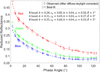 |
Fig. 5 Reduced reflectance after diffuse skylight correction and the corresponding best-fit results (example of Sol 32). The results are shown using the HG2 model. Diamond symbols represent the reduced reflectance values after diffuse skylight correction, while the dashed lines indicate the simulated phase curves generated with the best-fit photometric parameters, as listed in the figure. The three colors correspond to the Red, Green, and Blue bands, respectively. |
3 Results
The phase curves of reduced reflectance after diffuse skylight correction and the best-fit result are presented in Fig. 5, exemplified by Sol 32. The reduced reflectance is defined as the radiance factor (RADF) divided by the Lommel-Seeliger (LS) function (Hapke 1993), where LS = μ0/(μ0 + μ). The retrieved results from the five Zhurong datasets are shown in Appendix A. Among the photometric parameters, b and ω are relatively well constrained, with small uncertainties and convergence close to the optimal solution. When the dataset includes very small phase angles, the parameter h, representing the opposition effect width, is also well constrained (e.g., Sols 32 and 58). However, when small-angle observations are absent, the constraint on h becomes weaker. The parameters cb and ![Mathematical equation: $\[\bar{\theta}\]$](/articles/aa/full_html/2026/04/aa58201-25/aa58201-25-eq15.png) are less well constrained, showing relatively larger uncertainties.
are less well constrained, showing relatively larger uncertainties.
After performing parameter inversions using both the HG1 and HG2 models, we derived the corresponding single scattering albedo (SSA) values (as shown in Figure 6). The spectra from Sols 32, 58, and 84 are highly consistent, while Sol 99 exhibits slightly higher SSA. Soil near the lander on Sol 05 could not be constrained with HG1, but HG2 indicates notably higher SSA. All soils display an absorption feature near ~550 nm, associated with ferric materials (Farrand et al. 2008; Rice et al. 2022, 2023; Morris et al. 2000).
The relationship between the asymmetric parameter (ξ) and SSA (ω) is shown in Fig. 7. Positive ξ indicates a tendency toward forward scattering, while negative ξ indicates a tendency toward backscattering. The soils from Sols 32, 58, 84, and 99 are all predominantly backscattering, with Sol 99 exhibiting the weakest backscattering and Sol 58 the strongest. The uncertainty for Sol 84 is very small, with most solutions converging near the optimal value. For Sols 99 and 84, backscattering increases with SSA, whereas the trend is unclear for Sols 32 and 58 due to larger uncertainties.
The backscattering fraction (cb) versus the asymmetry parameter (b) for soils on five Sols retrieved using the HG2 model are shown in Fig. 8. The background values correspond to those of laboratory samples (McGuire & Hapke 1995; Johnson et al. 2013) and the global averages derived from orbital data inversion (Vincendon 2013). Sol 05 exhibits scattering properties that are significantly different from the other Sols and deviates from the classical L-shape region, indicating very strong forward scattering. In contrast, Sols 32, 58, 84, and 99 show a tendency toward backscattering, with scattering properties similar to spheres with high or moderate internal scattering and resembling laboratory samples HWMK 600 (150–1000 μm grain size, Johnson et al. 2013). Compared with Sols 32, 58, and 99, the backscattering of Sol 84 soil is weaker. With decreasing wavelength, b increases and cb decreases, indicating a weakening of the backscattering tendency. This trend is consistent with that observed for HWMK 600 (150–1000 μm grain size) over the similar wavelength range (450–750 nm).
Previous in situ and laboratory observations have shown that macroscopic roughness (![Mathematical equation: $\[\bar{\theta}\]$](/articles/aa/full_html/2026/04/aa58201-25/aa58201-25-eq16.png) ) tends to decrease with increasing single scattering albedo (ω) (Johnson et al. 2006a,b, 2015; Liang et al. 2020; Shepard & Helfenstein 2007). However, for the datasets used in this study, macroscopic roughness is more difficult to constrain than other parameters and thus exhibits large uncertainties. Consequently, except for Sol 05 under the HG2 model, the relationship between
) tends to decrease with increasing single scattering albedo (ω) (Johnson et al. 2006a,b, 2015; Liang et al. 2020; Shepard & Helfenstein 2007). However, for the datasets used in this study, macroscopic roughness is more difficult to constrain than other parameters and thus exhibits large uncertainties. Consequently, except for Sol 05 under the HG2 model, the relationship between ![Mathematical equation: $\[\bar{\theta}\]$](/articles/aa/full_html/2026/04/aa58201-25/aa58201-25-eq17.png) and ω is not clearly defined for the other Sols (as shown in Fig. 9). Considering the uncertainties,
and ω is not clearly defined for the other Sols (as shown in Fig. 9). Considering the uncertainties, ![Mathematical equation: $\[\bar{\theta}\]$](/articles/aa/full_html/2026/04/aa58201-25/aa58201-25-eq18.png) generally ranges between 0° and 15°.
generally ranges between 0° and 15°.
Since the opposition effect becomes significant only at very small phase angles, the inversion of the opposition effect width parameter (h) was performed only for the datasets that include phase angles below 20°. Fig. 10 presents the inversion results for the opposition effect width (h). In the HG1 results, the h values for RGB-band of soils on Sols 32 and 58 are similar, ranging from 0.04 to 0.06, while Sol 84 exhibits h values between 0.08 and 0.12. In the HG2 model, the h values for Sols 32 and 58 range from 0.03 to 0.05. For Sol 84, h is higher than for Sols 32 and 58, but the uncertainty is large, with possible values spanning 0.01–0.15, indicating weaker constraints.
To illustrate the phase reddening phenomenon, we took the ratio of the corrected RADF phase curves at different wavelengths, resulting in the ratio curves shown in Fig. 11. Scatter points represent the ratios of RADF values after atmospheric correction, and solid lines are second-order polynomial fits. The band ratio curves exhibit an arch shape, forming a convex profile. The peak phase angles are approximately 60° for Sols 32, 58,84, and 99, and about 68° for Sol 05.
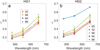 |
Fig. 6 Single scattering albedo versus wavelength. (a) HG1 model; (b) HG2 model. The error bars represent one standard deviation, and different colors correspond to the results from different Sols. |
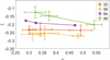 |
Fig. 7 HG1 asymmetric parameter versus single scattering albedo. The error bars represent one standard deviation, and different colors correspond to the results from different Sols. |
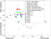 |
Fig. 8 Backscattering fraction (cb) versus asymmetry parameter (b). Gray symbols in the background represent cb of synthetic materials measured in the laboratory (McGuire & Hapke 1995), and black crosses denote the globally retrieved Martian scattering parameters (Vincendon 2013). The solid gray circle represents the Martian analog samples HWMK 600 (150–1000 μm grain size), with the cb values decreasing at wavelengths of 750, 950, 550, and 450 nm, respectively (Johnson et al. 2013). Colored symbols indicate the parameters retrieved from the Zhurong dataset for the three RGB bands. |
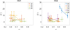 |
Fig. 9 Macroscopic roughness ( |
![Mathematical equation: $\[\bar{\theta}\]$](/articles/aa/full_html/2026/04/aa58201-25/aa58201-25-eq19.png)
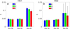 |
Fig. 10 Opposition effect width (h) values derived from the NaTeCam datasets. (a) Retrieved using the HG1 model; (b) retrieved using the HG2 model. |
4 Discussion
4.1 Single scattering albedo
Fig. 6 presents the retrieved SSA results. The SSA of the Sol 05 soil is significantly higher than that of the other Sols. The Sol 05 dataset covers an area located near the lander (white dashed box in Fig. 12b). Before landing, the surface materials appeared relatively homogeneous (Fig. 12a). Following landing, the descent engine plume removed the finer-grained, higher-albedo surface materials, exposing likely coarser-grained and lower-albedo subsurface materials. This process produced a darkened area approximately 100 m in diameter (Fig. 12b). Therefore, it is significantly different from the soils observed in the other datasets. Previous photometric studies of the Curiosity rover datasets also found that disturbed soils near the landing site (e.g., Sol 20) exhibited higher SSA compared to other soils (Johnson et al. 2022), consistent with the Zhurong results.
The SSA of Sol 99 is slightly higher than those of Sols 32, 58, and 84, which may be related to the presence of a nearby Transverse Aeolian Ridge (TAR). The defined soil ROI for Sol 99 may include partial contributions from the TAR, though further photometric studies are needed to confirm this. Soils from Sols 32, 58, and 84 are the most consistent, with SSA values ranging from 0.3 to 0.5, comparable to the dark soils in the Spirit landing site region (Johnson et al. 2006a, 2015, 2021). However, due to differences in band centers and widths, a direct comparison between NaTeCam and Pancam results is not straightforward. NaTeCam band centers and widths are similar to those of the Mars Hand Lens Imager (MAHLI) on board Curiosity, but the retrieved SSA of soils is lower than that retrieved from MAHLI (Liang et al. 2020).
Moreover, the SSA of Zhurong landing site soils is lower than that of traditional Mars analog soils such as JSC-1 and MGS, and is closer to that of HWMK 600 (150–1000 μm) (Johnson et al. 2013; Sun et al. 2023). This difference may be attributed not only to composition but also to particle size distribution. For the G band (~550 nm), the SSA spectra show a weak absorption feature, consistent with observations from the MSCam instrument on Zhurong (Zhang et al. 2022). This absorption is associated with Fe-oxides, and the absorption depth can be used to estimate the degree of Fe oxidation (Rice et al. 2022, 2023; Farrand et al. 2008; Morris et al. 2000). The SSA spectrum of Sol 05 is similar to that of the disturbed red and gray soil units in the Bradbury Landing region observed by Curiosity (Johnson et al. 2022), and exhibits a weaker absorption at 550 nm compared to the other Sols, suggesting that the subsurface soil may have a lower degree of Fe oxidation.
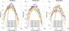 |
Fig. 11 Radiance factor (RADF) ratio for the phase curves of NaTeCam datasets. Scatter points represent the ratio of long-wavelength to short-wavelength bands for different Sols. RADF values are retrieved using the HG2 model and corrected for diffuse skylight. Solid lines indicate second-order polynomial fits to the datasets. |
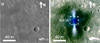 |
Fig. 12 Comparison of the Zhurong landing area before and after landing. (a) Pre-landing HiRIC image (HX1_GRAS_HIRIC_DIM_0.7_0004_251515N1095850E_A). (b) Post-landing HiRISE image (ESP_069665_2055_COLOR; linearly stretched with R: 640–728, G: 490–590, B: 55–85, respectively. The white dashed box outlines the area observed by NaTeCam during Sol 05 (Fig. B.1a). |
4.2 Phase function parameters
For the HG1 model, the asymmetric parameter ξ shows a clear backscattering behavior (ξ < 0) for all Sols except Sol 05, where the limited phase angle coverage prevents reliable inversion. This is consistent with previous in situ studies indicating that most Martian soils exhibit backscattering properties (Johnson et al. 2008). Sol 99 exhibits the weakest backscattering, which may be related to the area being close to Transverse Aeolian Ridges (TAR), containing partial TAR materials and higher soil cementation (Qin et al. 2023; Liu et al. 2023b). Similarly, Curiosity observed stronger backscattering in soils observed during the initial portion of the traverse and weaker backscattering near the outskirts of the Bagnold Dunes region, perhaps as a consequence of encountering possibly finer-grained soils (Johnson et al. 2022).
For the HG2 model, the b versus cb plot shows that Sol 05, affected by rover landing plume disturbance, deviates significantly from other Sols, exhibiting strong forward scattering and narrow-lobe characteristics. Similar behavior was observed for disturbed soils near the Curiosity landing site (Johnson et al. 2022). The landing plume likely removed surface dust and fine grains, exposing subsurface materials with scattering properties markedly different from the surface layer.
Sols 32–99 display clear backscattering properties, similar to Sphere moderate internal scattering and Sphere high internal scattering synthetic materials (McGuire & Hapke 1995), as well as the HWMK 600 (150–1000 μm) Martian simulant (Johnson et al. 2013). The exploration areas investigated by Opportunity, Spirit, and Curiosity are much larger than that of Zhurong, and they revealed a wide diversity of soil scattering properties. In comparison, the soils at the Zhurong landing site exhibit stronger backscattering characteristics than most soil types observed at the three previous landing sites, showing similarities only with a limited number of localized regions. The Zhurong site also appears to be more heavily covered by dust than those sites (as shown in Fig. 13), which may partly account for the enhanced backscattering properties of the local soils (Johnson et al. 2008).
Compared to global average scattering properties (Vincendon 2013), the Zhurong landing site soils show stronger backscattering and weaker narrow-lobe characteristics. Within the NaTeCam wavelength range, backscattering increases with increasing wavelength, which is consistent with the results for the Martian analog HWMK 600 (150–1000 μm) over the same range (Johnson et al. 2013). However, this does not imply that a monotonic increasing trend is present over a broader wavelength range. For example, the backscattering of HWMK 600 (150–1000 μm) at 950 nm is weaker than at 750 nm. Furthermore, previous studies of other laboratory synthetic samples also showed that b and cb vary with wavelength in a sample-dependent manner, without a universal trend (Johnson et al. 2013; Pilorget et al. 2016). Therefore, the observed increase of b and decrease of cb with wavelength at the Zhurong landing site likely applies only within the limited wavelength range of NaTeCam.
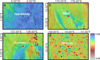 |
Fig. 13 Dust cover index (DCI) maps of the rover landing sites on Mars (data from Ruff & Christensen 2002). (a)–(d) correspond to the landing sites of Opportunity, Spirit, Curiosity, and Zhurong, respectively. Lower DCI values indicate higher dust coverage |
4.3 Opposition effect width
Fig. 10 shows the opposition effect width (h) derived from HG1 and HG2 models. The h value of Sol 84 is larger than that of Sol 32 and Sol 58, but with greater uncertainty. Considering that the minimum phase angle for Sol 84 is 15°, the results from Sol 32 and 58 may better represent the Zhurong landing site soil. The HG1-derived h values are around 0.05, whereas most regions observed by Spirit, Opportunity, and Curiosity exhibit h values greater than 0.05. The HG2-derived h values are around 0.04, close to the global average h (=0.05) obtained from orbital observations (Vincendon 2013). The opposition effect width h is mainly controlled by the porosity and/or particle size distribution of the medium. A porous internal structure and/or a wide range of particle sizes enhance the shadow-hiding effect at small phase angles, leading to a sharp increase in brightness (Helfenstein & Veverka 1987, 1989; Hapke 1993). Therefore, the relatively small value of h indicates that the soils at the Zhurong landing site possess higher porosity and/or a more heterogeneous particle size distribution. This interpretation is consistent with observations from Zhurong’s Micro-Image camera, which revealed that the particle size of surface soils is in the range of 1.5–2.5 mm (Zhao et al. 2023). However, these particles are in fact aggregates cemented from finer grains, suggesting that their internal structure is relatively loose and porous.
4.4 Macroscopic roughness
The macroscopic roughness (![Mathematical equation: $\[\bar{\theta}\]$](/articles/aa/full_html/2026/04/aa58201-25/aa58201-25-eq20.png) ) of Zhurong landing site soil derived from HG1 and HG2 models ranges from 0° to 15°, with relatively large uncertainties, indicating weak constraints on
) of Zhurong landing site soil derived from HG1 and HG2 models ranges from 0° to 15°, with relatively large uncertainties, indicating weak constraints on ![Mathematical equation: $\[\bar{\theta}\]$](/articles/aa/full_html/2026/04/aa58201-25/aa58201-25-eq21.png) . In previous studies of other landing areas, soils were consistently identified as the smoothest units with the lowest macroscopic roughness (Johnson et al. 2006a,b, 2015, 2021, 2022). Compared with these landing areas and the global average, the Zhurong landing area exhibits even lower macroscopic roughness, suggesting a smoother surface that may be related to enhanced dust coverage (Ruff & Christensen 2002). We also calculated the surface slope for all pixels within the selected ROIs, finding very limited variations, with a standard deviation of less than 5°. This result is consistent with the relatively low macroscopic roughness retrieved from photometric inversion. In the HG2 model, Sol 05 shows significantly higher
. In previous studies of other landing areas, soils were consistently identified as the smoothest units with the lowest macroscopic roughness (Johnson et al. 2006a,b, 2015, 2021, 2022). Compared with these landing areas and the global average, the Zhurong landing area exhibits even lower macroscopic roughness, suggesting a smoother surface that may be related to enhanced dust coverage (Ruff & Christensen 2002). We also calculated the surface slope for all pixels within the selected ROIs, finding very limited variations, with a standard deviation of less than 5°. This result is consistent with the relatively low macroscopic roughness retrieved from photometric inversion. In the HG2 model, Sol 05 shows significantly higher ![Mathematical equation: $\[\bar{\theta}\]$](/articles/aa/full_html/2026/04/aa58201-25/aa58201-25-eq22.png) compared to other Sols, likely due to the removal of fine surface dust and soil by the descent plume, exposing a coarser subsurface. Typically, SSA and
compared to other Sols, likely due to the removal of fine surface dust and soil by the descent plume, exposing a coarser subsurface. Typically, SSA and ![Mathematical equation: $\[\bar{\theta}\]$](/articles/aa/full_html/2026/04/aa58201-25/aa58201-25-eq23.png) are inversely related, as increased macroscopic roughness reduces multiple scattering (Shepard & Helfenstein 2007; Cord et al. 2003; Shkuratov et al. 2005). Except for Sol 05, this trend is not evident in the other Sols, possibly due to large uncertainties in
are inversely related, as increased macroscopic roughness reduces multiple scattering (Shepard & Helfenstein 2007; Cord et al. 2003; Shkuratov et al. 2005). Except for Sol 05, this trend is not evident in the other Sols, possibly due to large uncertainties in ![Mathematical equation: $\[\bar{\theta}\]$](/articles/aa/full_html/2026/04/aa58201-25/aa58201-25-eq24.png) .
.
4.5 Phase curve ratios
The phase curve ratios of soil from Sols 32–99 exhibit clear arch shapes. Second-order polynomial fits show peak values around 60°, consistent with soil observations by Curiosity MAHLI in the Kimberley region and laboratory sample AREF 238 (Liang et al. 2020; Johnson et al. 2013). The peak phase angle for Sol 05 is higher than those of the other Sols, occurring at approximately 68°, which is similar to values reported for the red rock at Rocknest and the regolith at Darwin observed by the Curiosity rover (Johnson et al. 2022). However, due to the limited phase angle coverage for Sol 05 and the poorer performance of the secondorder polynomial fit compared to the other sols, this peak value may not be entirely accurate.
This phase reddening phenomenon may be linked to volume scattering—at moderate phase angles, increased optical path lengths enhance volume scattering, producing phase reddening, whereas at higher phase angles, surface scattering becomes more dominant, leading to phase blueing (Adams & Filice 1967). The amplitude and position of the arch peak in phase ratios may be influenced by factors such as microstructural properties, spectral slope, and incidence geometry (Schröder et al. 2014; Johnson et al. 2013; Sun et al. 2023). However, the underlying causes remain complex and not yet well constrained. Due to the limited spatial and spectral coverage, and the similarity of photometric parameters across these Sols, no clear correlation between the arch peak phase angle and other parameters is observed. Laboratory studies suggest that peak positions may depend on the incidence angle (Sun et al. 2023), but this effect is not evident in Zhurong landing site soils. The ROI incidence angles for Sols 32, 58, and 99 are ~60–71°, whereas for Sol 84 are ~32–37°, yet their phase curve peak positions are similar, showing no significant difference. Yang et al. (2020) suggested that the spectral differences induced by phase reddening can be exploited to enhance the identification of surface features. For future observations at the Zhurong landing area and its surrounding areas, employing an observation geometry with a phase angle of around 60° in the visible wavelength range may help maximize the contrast of surface features and retrieve more information.
4.6 The photometric properties of Zhurong landing area
One of the main objectives of this study is to characterize the photometric properties of the Zhurong landing area, providing more accurate ground-truth data for refined quantitative studies using orbital remote sensing. We focused on the soil units that are most extensively distributed across the landing site, in order to represent the large-scale photometric properties of the region.
The Sol 05 dataset is located in an area affected by the lander’s engine plume, likely representing the photometric properties of the subsurface, which differ significantly from those observed on other Sols. Due to the limited phase angle coverage of this dataset, the inversion uncertainties are relatively large; therefore, its results are not considered in our analysis. The photometric properties derived from Sols 32, 58, and 84 are quite similar, showing no significant differences. This indicates that the selected soil units are representative, and the inverted parameters can reliably characterize the photometric properties of the area.
The SSA of Sol 99 is slightly higher than that of Sols 32, 58, and 84, and it exhibits slightly weaker backscattering, likely due to the study area of Sol 99 being close to TAR. The soil ROI may contain some components derived from the TAR, which is widely distributed across the landing site with scales ranging from tens to hundreds of meters (Liu et al. 2023a). Using a simple threshold-based segmentation, the area of TARs in Fig. 1b was extracted, occupying less than 2.8% of the study area. Therefore, for most orbital data, the influence of TARs is likely minor, and Sol 99 is not considered when evaluating the average photometric properties of the Zhurong landing site.
Considering the inversion results from Sols 32, 58, and 84, the surface at the landing site generally exhibits backscattering behavior, consistent with the overall backscattering nature of Martian surface (Johnson et al. 2008; Vincendon 2013). Compared with most soils observed by the MERs and Curiosity, the Zhurong landing site soils show stronger backscattering, which may be related to the relatively higher dust coverage in this region (Fig. 13; Ruff & Christensen 2002). The single scattering albedo in the visible wavelength range is between 0.3 and 0.5, the surface material has relatively high porosity and/or particle size distributions are variable, while the surface remains relatively smooth with low macroscopic roughness.
Although the datasets we used only cover approximately one kilometer, previous large-scale orbital spectral studies of this region have revealed that the spectral characteristics at the landing site and its surrounding areas are highly similar (Wu et al. 2021). This may be related to the widespread presence of similar Vastitas Borealis Formation materials or dust in the region, suggesting that the photometric properties of the landing area and its adjacent regions may also be similar.
Therefore, we used the averages of the RGB bands from the soil units of Sols 32, 58, and 84 to represent the photometric properties of the Zhurong landing site and its surrounding area. Among these, the h parameters (HG1 and HG2) and ![Mathematical equation: $\[\bar{\theta}\]$](/articles/aa/full_html/2026/04/aa58201-25/aa58201-25-eq25.png) (HG1) from Sol 84 were poorly constrained and were excluded when calculating the averages. Accordingly, we recommend the following photometric parameters for the Zhurong landing site and its surrounding areas:
(HG1) from Sol 84 were poorly constrained and were excluded when calculating the averages. Accordingly, we recommend the following photometric parameters for the Zhurong landing site and its surrounding areas:
HG1 model: ξ =
![Mathematical equation: $\[-0.23_{-0.02}^{+0.02}\]$](/articles/aa/full_html/2026/04/aa58201-25/aa58201-25-eq26.png) , B0 = 1, h =
, B0 = 1, h = ![Mathematical equation: $\[0.046_{-0.005}^{+0.005}\]$](/articles/aa/full_html/2026/04/aa58201-25/aa58201-25-eq27.png) ,
, ![Mathematical equation: $\[\bar{\theta} = 5_{~~-5^{\circ}}^{\circ+6^{\circ}}\]$](/articles/aa/full_html/2026/04/aa58201-25/aa58201-25-eq28.png) ;
;HG2 model: b =
![Mathematical equation: $\[0.33_{-0.02}^{+0.02}\]$](/articles/aa/full_html/2026/04/aa58201-25/aa58201-25-eq29.png) , cb =
, cb = ![Mathematical equation: $\[0.68_{-0.04}^{+0.04}\]$](/articles/aa/full_html/2026/04/aa58201-25/aa58201-25-eq30.png) , B0 = 1, h =
, B0 = 1, h = ![Mathematical equation: $\[0.041_{-0.004}^{+0.004}\]$](/articles/aa/full_html/2026/04/aa58201-25/aa58201-25-eq31.png) ,
, ![Mathematical equation: $\[\bar{\theta} = 3_{~~-3^{\circ}}^{\circ+5^{\circ}}\]$](/articles/aa/full_html/2026/04/aa58201-25/aa58201-25-eq32.png) .
.
Compared to the HG1 model, the HG2 model includes one additional parameter and provides a better fit to the phase curves at the landing area. Consistent with many previous spectral studies of Martian surface, we recommend using the HG2 model for modeling the reflectance behavior of the Martian surface.
In comparison with laboratory Mars analogs, the photometric behavior of the Zhurong landing area soils is found to be most consistent with that of the HWMK 600 (150–1000 μm) simulant, showing similar single-scattering albedo and backscattering characteristics. HWMK 600, sampled from the Mauna Kea Volcano, has been widely employed as an analog for Martian dust and weathered basaltic sand (Morris et al. 2000, 2001). We also compared the near-infrared spectra of HWMK 600 with those acquired by Zhurong. To ensure a robust comparison, all SWIR (Short Wavelength Infrared) spectra of soils acquired by Zhurong were photometrically corrected using the Hapke-derived parameters retrieved in this study and normalized to the RELAB observation geometry (i = 30°, e = 0°). As shown in Fig. 14, the red line represents the smoothed average spectrum of all soils at the Zhurong landing site, while the gray solid line and shaded area indicate the original average spectra and one-sigma standard deviation, respectively. The blue line corresponds to the RELAB spectrum of the HWMK 600 sample (ID: capa03, grain size 0–45 μm), convert to RADF by dividing by cos 30°. In the short-wavelength infrared range (0.85–2.4 μm), the Zhurong soil spectra also closely resemble those of HWMK 600, with absorption features at ~940, ~1450, ~1940, and ~2220 nm. This similarity suggests that the landing area materials and HWMK 600 may share comparable origins and/or alteration histories. We therefore propose that HWMK 600 could serve as a primary component in constructing simulants of soils from the Zhurong landing area.
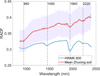 |
Fig. 14 Comparison between the mean soil spectrum at the Zhurong landing site and the HWMK 600 spectrum. The red line represents the mean soil spectrum acquired by Zhurong (smoothed and photometrically corrected to i = 30° and e = 0°). The gray line denotes the unsmoothed spectra, while the shaded area indicates one standard deviation. The blue line corresponds to the HWMK 600 spectrum (RELAB ID: capa03, grain size 0–45 μm), converted to RADF by dividing by cos 30°. |
5 Conclusion
In this study, we conducted photometric analyses of the widely distributed soil units in the Zhurong landing area based on multiphase angle observations acquired by NaTeCam, and for the first time obtained the photometric properties of this region. Five Martian days of data were selected for analysis. These datasets were acquired by NaTeCam through 360° panoramas within a very short time interval, which maximized the phase angle coverage while minimizing interferences caused by variations in atmospheric conditions and illumination. We constructed a digital elevation model (DEM) corresponding to the dataset to obtain the illumination geometry of the study area. Based on this geometry, we extracted the phase curves of the soil units and performed sky-scattered light correction using a sky brightness model generated by the DISORT model under the corresponding observation conditions. Subsequently, employing the Hapke radiative transfer model together with a parallel Monte Carlo inversion framework combined with a simulated annealing algorithm, we retrieved the photometric and microphysical properties of the soil units. Our main findings are summarized as follows:
The surface soils at the landing site exhibit a stronger backscattering tendency than those at other landing areas, with relatively high porosity and/or heterogeneous particle size distribution, and low macroscopic roughness. Some units may have been affected by nearby TARs, resulting in weaker backscattering. In contrast, soils in the vicinity of the lander, which were influenced by plume–surface interactions during landing, show higher single scattering albedo, larger macroscopic roughness, and a pronounced forward-scattering behavior, possibly reflecting the photometric properties of subsurface materials.
The surface soils display a pronounced phase reddening effect, with the ratio peak occurring at ~60°, suggesting that observations at this phase angle may maximize spectral contrasts across the landing site. This provides valuable guidance for optimizing viewing geometries in future orbital observations of this region.
-
We recommend the following photometric parameters for correcting spectra acquired at and around the Zhurong landing area:
HG1 model: ξ =
![Mathematical equation: $\[-0.23_{-0.02}^{+0.02}\]$](/articles/aa/full_html/2026/04/aa58201-25/aa58201-25-eq33.png) , B0 = 1, h =
, B0 = 1, h = ![Mathematical equation: $\[0.046_{-0.005}^{+0.005}\]$](/articles/aa/full_html/2026/04/aa58201-25/aa58201-25-eq34.png) ,
, ![Mathematical equation: $\[\bar{\theta} = 5_{~~-5^{\circ}}^{\circ+6^{\circ}}\]$](/articles/aa/full_html/2026/04/aa58201-25/aa58201-25-eq35.png) ;
;HG2 model: b =
![Mathematical equation: $\[0.33_{-0.02}^{+0.02}\]$](/articles/aa/full_html/2026/04/aa58201-25/aa58201-25-eq36.png) , cb =
, cb = ![Mathematical equation: $\[0.68_{-0.04}^{+0.04}\]$](/articles/aa/full_html/2026/04/aa58201-25/aa58201-25-eq37.png) , B0 = 1, h =
, B0 = 1, h = ![Mathematical equation: $\[0.041_{-0.004}^{+0.004}\]$](/articles/aa/full_html/2026/04/aa58201-25/aa58201-25-eq38.png) ,
, ![Mathematical equation: $\[\bar{\theta} = 3_{~~-3^{\circ}}^{\circ+5^{\circ}}\]$](/articles/aa/full_html/2026/04/aa58201-25/aa58201-25-eq39.png) .
.
The HG2 model yields better fits and is therefore preferred. Using these parameters, we also applied photometric corrections to all SWIR spectra of soils acquired by Zhurong.
The photometric properties of the Zhurong soils most closely resemble those of the Martian analog HWMK 600. Furthermore, the near-infrared spectra of HWMK 600 shows strong similarities to the corrected SWIR spectra of soils from Zhurong. These results suggest that HWMK 600 represents a strong candidate for preparing soil simulants of the Zhurong landing area.
These results provide new in situ constraints on photometric behavior in the Zhurong landing area. Future work will extend the photometric investigation to additional surface units at the Zhurong area, aiming to refine our understanding of the local photometric characteristics and provide further ground-truth constraints for Martian photometric studies.
Acknowledgements
We thank Dr. Jeffrey Johnson for constructive reviews that significantly improved the quality of this manuscript. We are also grateful to the Tianwen-1 mission team for their outstanding work and the China National Space Administration (CNSA) for providing the Tianwen-1 data used in this study. This research was supported by the National Natural Science Foundation of China (42430210, 42441832), the Key Technology Research Project of TW-3 (TW3004), the International Technical Cooperation Research (Aerospace) ZA09 and the China Scholarship Council (CSC) Joint PhD Program (No. 202304910540). Xing Wu also acknowledges support from the Young Elite Scientists Sponsorship Program by the China Association for Science and Technology (Grant No. 2022QNRC001). We also thank Dr. Mathieu Vincendon, Dr. John Carter, Dr. Te Jiang, and Dr. Mark Lemmon for valuable discussions and insights that contributed to this work.
References
- Adams, J. B., & Filice, A. L. 1967, J. Geophys. Res., 72, 5705 [NASA ADS] [CrossRef] [Google Scholar]
- Arvidson, R. E., Gooding, J. L., & Moore, H. J. 1989a, Rev. Geophys., 27, 39 [Google Scholar]
- Arvidson, R. E., Guinness, E. A., Dale-Bannister, M. A., et al. 1989b, J. Geophys. Res., 94, 1573 [Google Scholar]
- Audouard, J., Poulet, F., Vincendon, M., et al. 2014, J. Geophys. Res. Planets, 119, 1969 [Google Scholar]
- Bell, J. F., McSween, H. Y., Crisp, J. A., et al. 2000, J. Geophys. Res., 105, 1721 [Google Scholar]
- Cord, A. M., Pinet, P. C., Daydou, Y., & Chevrel, S. D. 2003, Icarus, 165, 414 [Google Scholar]
- Domingue, D., Hartman, B., & Verbiscer, A. 1997, Icarus, 128, 28 [Google Scholar]
- Farrand, W. H., Bell, J. F., Johnson, J. R., et al. 2008, J. Geophys. Res. Planets, 113, E12S38 [Google Scholar]
- Fernando, J., Schmidt, F., Ceamanos, X., et al. 2013, J. Geophys. Res. Planets, 118, 534 [NASA ADS] [CrossRef] [Google Scholar]
- Fernando, J., Schmidt, F., Pilorget, C., et al. 2015, Icarus, 253, 271 [NASA ADS] [CrossRef] [Google Scholar]
- Fernando, J., Schmidt, F., & Douté, S. 2016, Planet. Space Sci., 128, 30 [Google Scholar]
- Fornasier, S., Hasselmann, P. H., Deshapriya, J. D. P., et al. 2020, A&A, 644, A142 [NASA ADS] [CrossRef] [EDP Sciences] [Google Scholar]
- Gehrels, T., Coffeen, T., & Owings, D. 1964, AJ, 69, 826 [NASA ADS] [CrossRef] [Google Scholar]
- Guinness, E. A. 1981, J. Geophys. Res., 86, 7983 [Google Scholar]
- Guinness, E. A., Arvidson, R. E., Clark, I. H. D., & Shepard, M. K. 1997, J. Geophys. Res., 102, 28687 [Google Scholar]
- Hapke, B. 1993, Theory of reflectance and emittance spectroscopy (Cambridge University Press) [Google Scholar]
- Helfenstein, P., & Veverka, J. 1987, Icarus, 72, 342 [NASA ADS] [CrossRef] [Google Scholar]
- Helfenstein, P., & Veverka, J. 1989, in Asteroids II, eds. R. P. Binzel, T. Gehrels, & M. S. Matthews, 557 [Google Scholar]
- Jiang, T., Hu, X., Zhang, H., et al. 2021, A&A, 646, A2 [NASA ADS] [CrossRef] [EDP Sciences] [Google Scholar]
- Jin, W., Zhang, H., Yuan, Y., et al. 2015, Geophys. Res. Lett., 42, 8312 [NASA ADS] [CrossRef] [Google Scholar]
- Johnson, J. R., Bridges, N. T., Anderson, R., et al. 1999, J. Geophys. Res., 104, 8809 [Google Scholar]
- Johnson, J. R., Grundy, W. M., Lemmon, M. T., et al. 2006a, J. Geophys. Res. Planets, 111, E02S14 [Google Scholar]
- Johnson, J. R., Grundy, W. M., Lemmon, M. T., et al. 2006b, J. Geophys. Res. Planets, 111, E12S16 [Google Scholar]
- Johnson, J. R., Bell, III, J. F., Geissler, P., et al. 2008, in The Martian Surface – Composition, Mineralogy, and Physical Properties, ed. J. Bell, III, 428 [Google Scholar]
- Johnson, J. R., Shepard, M. K., Grundy, W. M., Paige, D. A., & Foote, E. J. 2013, Icarus, 223, 383 [NASA ADS] [CrossRef] [Google Scholar]
- Johnson, J. R., Grundy, W. M., Lemmon, M. T., Bell, J. F., & Deen, R. G. 2015, Icarus, 248, 25 [Google Scholar]
- Johnson, J. R., Grundy, W. M., Lemmon, M. T., et al. 2021, Icarus, 357, 114261 [NASA ADS] [CrossRef] [Google Scholar]
- Johnson, J. R., Grundy, W. M., Lemmon, M. T., et al. 2022, Planet. Space Sci., 222, 105563 [Google Scholar]
- Kirkpatrick, S., Gelatt, C. D., & Vecchi, M. P. 1983, Science, 220, 671 [Google Scholar]
- Lemmon, M. T., Wolff, M. J., Smith, M. D., et al. 2004, Science, 306, 1753 [Google Scholar]
- Liang, W., Johnson, J. R., Hayes, A. G., et al. 2020, Icarus, 335, 113361 [Google Scholar]
- Liang, X., Chen, W., Cao, Z., et al. 2021, Space Sci. Rev., 217, 37 [Google Scholar]
- Lin, H., Yang, Y., Lin, Y., et al. 2020, A&A, 638, A35 [NASA ADS] [CrossRef] [EDP Sciences] [Google Scholar]
- Liu, W. C., & Wu, B. 2023, ISPRS J. Photogramm. Remote Sens., 204, 237 [Google Scholar]
- Liu, Y., Glotch, T. D., Scudder, N. A., et al. 2016, J. Geophys. Res. Planets, 121, 2004 [Google Scholar]
- Liu, J., Li, C., Zhang, R., et al. 2022a, Nat. Astron., 6, 65 [Google Scholar]
- Liu, Y., Wu, X., Zhao, Y.-Y. S., et al. 2022b, Sci. Adv., 8, eabn8555 [Google Scholar]
- Liu, J., Liu, Y., Wan, W., et al. 2023a, J. Geophys. Res. Planets, 128, e2023JE007857 [Google Scholar]
- Liu, J., Qin, X., Ren, X., et al. 2023b, Nature, 620, 303 [Google Scholar]
- McGuire, A. F., & Hapke, B. W. 1995, Icarus, 113, 134 [NASA ADS] [CrossRef] [Google Scholar]
- Milliken, R. E., Mustard, J. F., Poulet, F., et al. 2007, J. Geophys. Res. Planets, 112, E08S07 [Google Scholar]
- Moores, J. E., Ha, T., Lemmon, M. T., & Gunnlaugsson, H. P. 2015, Planet. Space Sci., 116, 6 [Google Scholar]
- Morris, R. V., Golden, D. C., Bell, J. F., et al. 2000, J. Geophys. Res., 105, 757 [Google Scholar]
- Morris, R. V., Graff, T. G., & Mertzman, S. A. 2001, J. Geophys. Res., 106, 5057 [Google Scholar]
- Mosegaard, K., & Tarantola, A. 1995, J. Geophys. Res., 100, 12431 [Google Scholar]
- Ockert-Bell, M. E., Bell, J. F., Pollack, J. B., McKay, C. P., & Forget, F. 1997, J. Geophys. Res., 102, 9039 [Google Scholar]
- Pilorget, C., Fernando, J., Ehlmann, B. L., Schmidt, F., & Hiroi, T. 2016, Icarus, 267, 296 [NASA ADS] [CrossRef] [Google Scholar]
- Pollack, J. B., Ockert-Bell, M. E., & Shepard, M. K. 1995, J. Geophys. Res., 100, 5235 [Google Scholar]
- Pommerol, A., Thomas, N., Jost, B., et al. 2013, J. Geophys. Res. Planets, 118, 2045 [Google Scholar]
- Qin, X., Ren, X., Wang, X., et al. 2023, Sci. Adv., 9, eadd8868 [Google Scholar]
- Rice, M. S., Seeger, C., Bell, J., et al. 2022, J. Geophys. Res. Planets, 127, e07134 [Google Scholar]
- Rice, M. S., Johnson, J. R., Million, C. C., et al. 2023, J. Geophys. Res. Planets, 128, e2022JE007548 [Google Scholar]
- Ruesch, O., Hiesinger, H., Cloutis, E., et al. 2015, Icarus, 258, 384 [Google Scholar]
- Ruff, S. W., & Christensen, P. R. 2002, J. Geophys. Res. Planets, 107, 5127 [Google Scholar]
- Schmidt, F., & Fernando, J. 2015, Icarus, 260, 73 [NASA ADS] [CrossRef] [Google Scholar]
- Schmidt, F., & Bourguignon, S. 2019, Icarus, 317, 10 [NASA ADS] [CrossRef] [Google Scholar]
- Schröder, S. E., Grynko, Y., Pommerol, A., et al. 2014, Icarus, 239, 201 [Google Scholar]
- Shaw, A., Wolff, M. J., Seelos, F. P., Wiseman, S. M., & Cull, S. 2013, J. Geophys. Res. Planets, 118, 1699 [Google Scholar]
- Shepard, M. K., & Helfenstein, P. 2007, J. Geophys. Res. Planets, 112, E03001 [Google Scholar]
- Shkuratov, Y. G., Stankevich, D. G., Petrov, D. V., et al. 2005, Icarus, 173, 3 [Google Scholar]
- Soderblom, J. M., Bell, J. F., Arvidson, R. E., et al. 2004, in AGU Fall Meeting Abstracts, 2004, AGU Fall Meeting Abstracts, P21A-0198 [Google Scholar]
- Stamnes, K., Tsay, S. C., Jayaweera, K., & Wiscombe, W. 1988, Appl. Opt., 27, 2502 [NASA ADS] [CrossRef] [Google Scholar]
- Sun, Y., Jiang, T., Zhuang, Y., et al. 2023, Planet. Space Sci., 227, 105639 [Google Scholar]
- Thomas, N. 2001, in Solar and Extra-solar Planetary Systems, 577, eds. I. P. Williams, & N. Thomas, 191 [Google Scholar]
- Tomasko, M. G., Doose, L. R., Lemmon, M., Smith, P. H., & Wegryn, E. 1999, J. Geophys. Res., 104, 8987 [Google Scholar]
- Vincendon, M. 2013, Planet. Space Sci., 76, 87 [Google Scholar]
- Vincendon, M., Langevin, Y., Poulet, F., Bibring, J.-P., & Gondet, B. 2007, J. Geophys. Res. Planets, 112, E08S13 [CrossRef] [Google Scholar]
- Wolff, M. J., Smith, M. D., Clancy, R. T., et al. 2009, J. Geophys. Res. Planets, 114, E00D04 [Google Scholar]
- Wu, X., Liu, Y., Zhang, C., et al. 2021, Icarus, 370, 114657 [Google Scholar]
- Yang, Y., Ma, P., Qiao, L., et al. 2020, A&A, 644, A30 [NASA ADS] [CrossRef] [EDP Sciences] [Google Scholar]
- Zhang, Q., Liu, D., Liu, J., et al. 2022, Icarus, 387, 115208 [Google Scholar]
- Zhang, Q., Liu, D., Ren, X., et al. 2023, Geophys. Res. Lett., 50, e2023GL104676 [Google Scholar]
- Zhao, Y.-Y. S., Yu, J., Wei, G., et al. 2023, Natl. Sci. Rev., 10, nwad056 [Google Scholar]
- Zhou, X., Liu, Y., Wu, X., Zhao, Z., & Zou, Y. 2023, Earth Planet. Phys., 7, 347 [Google Scholar]
Appendix A Photometric results retrieved from the five Zhurong NaTeCam dataset
All values following the ± symbol represenin parentheses indicate 1σ uncertainties. For ![Mathematical equation: $\[\bar{\theta}\]$](/articles/aa/full_html/2026/04/aa58201-25/aa58201-25-eq40.png) , negative values are nonphysical and should be interpreted as
, negative values are nonphysical and should be interpreted as ![Mathematical equation: $\[\bar{\theta}\]$](/articles/aa/full_html/2026/04/aa58201-25/aa58201-25-eq41.png) ≥ 0. (−−) indicates that the parameter could not be well constrained by the dataset;HG1 = 1-term Henyey-Greenstein function; HG2 = 2-term Henyey-Greenstein function.
≥ 0. (−−) indicates that the parameter could not be well constrained by the dataset;HG1 = 1-term Henyey-Greenstein function; HG2 = 2-term Henyey-Greenstein function.
Hapke parameters for the NaTeCam Sol 05 dataset, soil
Hapke parameters for the NaTeCam Sol 32 dataset, soil
Hapke parameters for the NaTeCam Sol 58 dataset, soil
Hapke parameters for the NaTeCam Sol 84 dataset, soil
Hapke parameters for the NaTeCam Sol 99 dataset, soil
Appendix B ROIs selection and phase curve extraction
The selected regions of interest (ROIs) locations and their corresponding zoomed-in views for Sols 05–99 are shown in Figs. B.1–B.5. Fig. B.6 presents the Digital Elevation Model (DEM), phase angle distributions, and the corresponding extracted phase curves for the four Sols other than Sol 32.
For Sol 05 in particular, darkened areas scorched by the lander’s rocket plume exhaust (Fig. B.1f) and regions containing abundant pebbles (Fig. B.1e) were avoided. The region outlined by the red box in Fig. B.1a may have been directly scoured by the lander’s secondary engines and appears darker than the surrounding terrain, potentially exposing deeper subsurface materials. However, this area covers only a limited phase angle range, which precludes reliable photometric parameter retrieval. Therefore, it was also excluded from the ROIs selection.
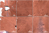 |
Fig. B.1 Distribution of regions of interest (ROIs) for Sol 05. (a) Digital Orthophoto Map (DOM) with a spatial resolution of 2 cm per pixel. (b–f) Zoomed-in views corresponding to the white dashed boxes in (a). White solid boxes indicate the ROIs used for phase-curve extraction. The red dashed box may correspond to deeper subsurface materials but covers a limited phase angle range and was therefore excluded from this study. White dashed lines indicate the mosaicking boundaries of the panoramic images. |
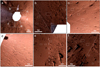 |
Fig. B.2 ROI distribution for Sol 32. The boxes and dashed lines denote the same features as in Fig. B.1 |
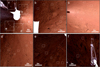 |
Fig. B.3 ROI distribution for Sol 58. The boxes and dashed lines denote the same features as in Fig. B.1 |
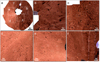 |
Fig. B.4 ROI distribution for Sol 84. The boxes and dashed lines denote the same features as in Fig. B.1 |
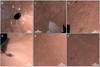 |
Fig. B.5 ROI distribution for Sol 99. The boxes and dashed lines denote the same features as in Fig. B.1 |
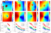 |
Fig. B.6 Digital Elevation Model (DEM, top), phase angle distributions (middle), and extracted phase curves (bottom) for Sols 05, 58, 84, and 99. White boxes in the top and middle panels indicate the ROIs corresponding to the phase curves shown in the bottom panel. |
Appendix C Influence of incomplete phase angle coverage on the inversion results
Owing to the limited phase angle coverage of the dataset, some photometric parameters cannot be well constrained, which consequently affects the robustness of the inversion results. To quantitatively evaluate the influence of phase angle coverage on the parameter inversion, we performed a simple simulation test. We assumed a reference surface with photometric parameters consistent with those retrieved for the Sol 32 R-band observations, namely b = 0.28, cb = 0.85, ![Mathematical equation: $\[\bar{\theta}\]$](/articles/aa/full_html/2026/04/aa58201-25/aa58201-25-eq75.png) = 1°, h = 0.04, and ω = 0.50. The relative azimuth angle between the incidence and emission directions was fixed at 170°. Both the incidence and emission angles were varied from 1° to 89°, resulting in a synthetic phase angle range of approximately 2°−170°.
= 1°, h = 0.04, and ω = 0.50. The relative azimuth angle between the incidence and emission directions was fixed at 170°. Both the incidence and emission angles were varied from 1° to 89°, resulting in a synthetic phase angle range of approximately 2°−170°.
Using both the Hapke model and the HG2 phase function, we simulated the corresponding reduced reflectance under these conditions. In order to isolate the sensitivity of each parameter, only one photometric parameter was varied at a time while keeping the others fixed. The results are shown in Fig. C.1, extending the phase angle range beyond that of Sol 32.
The simulations demonstrate that the parameter b primarily affects the phase curve at small phase angles (e.g., < 50°), and even a change of 0.02 in b produces a pronounced variation in the phase curve. Since the phase angle range of our study (3°−124°) includes this sensitive region, b is relatively well constrained, resulting in a high confidence level and small uncertainty. In contrast, variations in cb (e.g., by 0.05) significantly influence not only the small phase angle region but also the large phase angle behavior approaching 180°, which provides strong constraints on cb when such data are available. However, because our dataset lacks phase angles beyond ~125°, the constraint on cb is weaker, and the retrieved uncertainty for cb is correspondingly larger (approximately ~0.05).
The simulations further indicate that the parameter h is more strongly constrained by data at small phase angles (≤ 20°), whereas the macroscopic roughness parameter ![Mathematical equation: $\[\bar{\theta}\]$](/articles/aa/full_html/2026/04/aa58201-25/aa58201-25-eq76.png) is better constrained by large phase angle observations. The single-scattering albedo ω is primarily constrained by the overall amplitude of the phase curve.Therefore, incorporating observations at large phase angles (e.g., > 120°) would significantly improve the constraints on cb and
is better constrained by large phase angle observations. The single-scattering albedo ω is primarily constrained by the overall amplitude of the phase curve.Therefore, incorporating observations at large phase angles (e.g., > 120°) would significantly improve the constraints on cb and ![Mathematical equation: $\[\bar{\theta}\]$](/articles/aa/full_html/2026/04/aa58201-25/aa58201-25-eq77.png) .
.
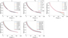 |
Fig. C.1 Influence of individual photometric parameters on the phase curves. The asterisk in the legend denotes the best-fit solution retrieved for the Sol 32 R band. Panels (a–e) show simulations in which only one parameter is varied at a time while all other parameters are fixed at their best-fit values. The vertical dashed line indicates the maximum observed phase angle for Sol 32; phase angles to the left correspond to the measured range, whereas those to the right represent the extrapolated range. |
We employed a parallel Monte Carlo inversion model to explore the parameter space and obtain multiple acceptable combinations of photometric parameters. Fig. C.2 shows the simulated phase curves corresponding to all acceptable solutions within the uncertainty range for Sol 32. These parameter combinations provide similarly good fits to the observed phase curves within the observed phase angle range, while exhibiting some variability outside this range. Such variability partially compensates for the limited phase angle coverage and may encompass the true phase curve behavior at unobserved phase angles.
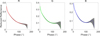 |
Fig. C.2 Simulated phase curves extrapolated beyond the observed phase angle range. The solid line represents the best-fit solution obtained from the inversion of the Sol 32 dataset, while the dashed line shows the extrapolation of this best-fit solution outside the observed phase angle range. The gray shaded area in the background indicates the simulated phase curves corresponding to all acceptable solutions within the uncertainty range derived from the parallel Monte Carlo inversion. |
All Tables
All Figures
|
Fig. 1 Location of the Zhurong landing site and NaTeCam datasets. (a) Location of the Zhurong landing site, overlaid on a MOLA digital terrain model. (b) Traverse path of Zhurong and locations of the acquired panoramic NaTeCam datasets, overlaid on a Tianwen-1 High-Resolution Imaging Camera (HiRIC) image (HX1_GRAS_HIRIC_DIM_0.7_0004_251515N1095850E_A). (c) Zhurong rover selfie and the position of NaTeCam on the rover; the selfie was taken by a small detachable camera carried by the rover. (d) 360° panoramic image acquired by NaTeCam on Sol 32. |
| In the text | |
|
Fig. 2 Photometry QUBs of the study area (Sol 32). The X-axis increases eastward, and the Y-axis increases northward, with the origin at the NaTeC am camera position. (a) Relative elevation with respect to NaTeCam. (b) Incidence angle. (c) Emission angle. (d) Phase angle. |
| In the text | |
|
Fig. 3 DOMs and extracted phase curves of Sol 32. (a) DOMs for Sols 32. The white dashed lines indicate the boundaries of the mosaicking, and the white boxes mark the selected ROIs. The red dashed line encloses the area affected by reflections from the rover’s coating. (b) The corresponding phase curves extracted from the ROIs. |
| In the text | |
|
Fig. 4 Sky brightness model and schematic of the radiative transfer process. (a) Sky brightness model Isky(θ, ϕ) generated by DISORT (Sol 32, R band). (b) Schematic of the radiative transfer at the Martian surface. The radiance received by NaTeCam consists of both direct solar light and diffuse skylight. |
| In the text | |
|
Fig. 5 Reduced reflectance after diffuse skylight correction and the corresponding best-fit results (example of Sol 32). The results are shown using the HG2 model. Diamond symbols represent the reduced reflectance values after diffuse skylight correction, while the dashed lines indicate the simulated phase curves generated with the best-fit photometric parameters, as listed in the figure. The three colors correspond to the Red, Green, and Blue bands, respectively. |
| In the text | |
|
Fig. 6 Single scattering albedo versus wavelength. (a) HG1 model; (b) HG2 model. The error bars represent one standard deviation, and different colors correspond to the results from different Sols. |
| In the text | |
|
Fig. 7 HG1 asymmetric parameter versus single scattering albedo. The error bars represent one standard deviation, and different colors correspond to the results from different Sols. |
| In the text | |
|
Fig. 8 Backscattering fraction (cb) versus asymmetry parameter (b). Gray symbols in the background represent cb of synthetic materials measured in the laboratory (McGuire & Hapke 1995), and black crosses denote the globally retrieved Martian scattering parameters (Vincendon 2013). The solid gray circle represents the Martian analog samples HWMK 600 (150–1000 μm grain size), with the cb values decreasing at wavelengths of 750, 950, 550, and 450 nm, respectively (Johnson et al. 2013). Colored symbols indicate the parameters retrieved from the Zhurong dataset for the three RGB bands. |
| In the text | |
|
Fig. 9 Macroscopic roughness ( |
| In the text | |
|
Fig. 10 Opposition effect width (h) values derived from the NaTeCam datasets. (a) Retrieved using the HG1 model; (b) retrieved using the HG2 model. |
| In the text | |
|
Fig. 11 Radiance factor (RADF) ratio for the phase curves of NaTeCam datasets. Scatter points represent the ratio of long-wavelength to short-wavelength bands for different Sols. RADF values are retrieved using the HG2 model and corrected for diffuse skylight. Solid lines indicate second-order polynomial fits to the datasets. |
| In the text | |
|
Fig. 12 Comparison of the Zhurong landing area before and after landing. (a) Pre-landing HiRIC image (HX1_GRAS_HIRIC_DIM_0.7_0004_251515N1095850E_A). (b) Post-landing HiRISE image (ESP_069665_2055_COLOR; linearly stretched with R: 640–728, G: 490–590, B: 55–85, respectively. The white dashed box outlines the area observed by NaTeCam during Sol 05 (Fig. B.1a). |
| In the text | |
|
Fig. 13 Dust cover index (DCI) maps of the rover landing sites on Mars (data from Ruff & Christensen 2002). (a)–(d) correspond to the landing sites of Opportunity, Spirit, Curiosity, and Zhurong, respectively. Lower DCI values indicate higher dust coverage |
| In the text | |
|
Fig. 14 Comparison between the mean soil spectrum at the Zhurong landing site and the HWMK 600 spectrum. The red line represents the mean soil spectrum acquired by Zhurong (smoothed and photometrically corrected to i = 30° and e = 0°). The gray line denotes the unsmoothed spectra, while the shaded area indicates one standard deviation. The blue line corresponds to the HWMK 600 spectrum (RELAB ID: capa03, grain size 0–45 μm), converted to RADF by dividing by cos 30°. |
| In the text | |
|
Fig. B.1 Distribution of regions of interest (ROIs) for Sol 05. (a) Digital Orthophoto Map (DOM) with a spatial resolution of 2 cm per pixel. (b–f) Zoomed-in views corresponding to the white dashed boxes in (a). White solid boxes indicate the ROIs used for phase-curve extraction. The red dashed box may correspond to deeper subsurface materials but covers a limited phase angle range and was therefore excluded from this study. White dashed lines indicate the mosaicking boundaries of the panoramic images. |
| In the text | |
|
Fig. B.2 ROI distribution for Sol 32. The boxes and dashed lines denote the same features as in Fig. B.1 |
| In the text | |
|
Fig. B.3 ROI distribution for Sol 58. The boxes and dashed lines denote the same features as in Fig. B.1 |
| In the text | |
|
Fig. B.4 ROI distribution for Sol 84. The boxes and dashed lines denote the same features as in Fig. B.1 |
| In the text | |
|
Fig. B.5 ROI distribution for Sol 99. The boxes and dashed lines denote the same features as in Fig. B.1 |
| In the text | |
|
Fig. B.6 Digital Elevation Model (DEM, top), phase angle distributions (middle), and extracted phase curves (bottom) for Sols 05, 58, 84, and 99. White boxes in the top and middle panels indicate the ROIs corresponding to the phase curves shown in the bottom panel. |
| In the text | |
|
Fig. C.1 Influence of individual photometric parameters on the phase curves. The asterisk in the legend denotes the best-fit solution retrieved for the Sol 32 R band. Panels (a–e) show simulations in which only one parameter is varied at a time while all other parameters are fixed at their best-fit values. The vertical dashed line indicates the maximum observed phase angle for Sol 32; phase angles to the left correspond to the measured range, whereas those to the right represent the extrapolated range. |
| In the text | |
|
Fig. C.2 Simulated phase curves extrapolated beyond the observed phase angle range. The solid line represents the best-fit solution obtained from the inversion of the Sol 32 dataset, while the dashed line shows the extrapolation of this best-fit solution outside the observed phase angle range. The gray shaded area in the background indicates the simulated phase curves corresponding to all acceptable solutions within the uncertainty range derived from the parallel Monte Carlo inversion. |
| In the text | |
Current usage metrics show cumulative count of Article Views (full-text article views including HTML views, PDF and ePub downloads, according to the available data) and Abstracts Views on Vision4Press platform.
Data correspond to usage on the plateform after 2015. The current usage metrics is available 48-96 hours after online publication and is updated daily on week days.
Initial download of the metrics may take a while.