| Issue |
A&A
Volume 708, April 2026
|
|
|---|---|---|
| Article Number | A58 | |
| Number of page(s) | 12 | |
| Section | Galactic structure, stellar clusters and populations | |
| DOI | https://doi.org/10.1051/0004-6361/202558290 | |
| Published online | 31 March 2026 | |
GALACTICNUCLEUS: A high-angular-resolution JHKs imaging survey of the Galactic center
V. Toward the GNS second data release: Methodology and photometric and astrometric performance
1
Instituto de Astrofísica de Andalucía (CSIC),
Glorieta de la Astronomía s/n,
18008
Granada,
Spain
2
Laboratoire d’Astrophysique de Bordeaux (LAB), Université de Bordeaux,
Bât. B18N, Allée Geoffroy Saint-Hilaire CS 50023,
33615
Pessac Cedex,
France
★ Corresponding author: This email address is being protected from spambots. You need JavaScript enabled to view it.
Received:
27
November
2025
Accepted:
19
February
2026
Abstract
Context. The center of the Milky Way presents a unique environment of fundamental astrophysical interest. However, its extreme crowding and extinction make this region particularly challenging to study. The GALACTICNUCLEUS survey, a high-angularresolution near-infrared imaging program, was designed to overcome these difficulties. Its first data release provides a powerful resource for exploring the Galactic center and enables key discoveries in this extreme environment.
Aims. We present the methodology and first results of a second data release of the GALACTICNUCLEUS survey, which incorporates significant improvements in data reduction, calibration, and methodology as well as a second epoch. In particular, we aim to provide deeper photometry, improved astrometry, and high-precision proper motion for the test fields analyzed in this study.
Methods. Observations were obtained with VLT/HAWK-I over two epochs separated by approximately seven years for most pointings and by four to five years for others. The data were acquired using speckle holography, and in the case of the second epoch, a ground-layer adaptive optics system was also employed. We have developed a new reduction pipeline with key improvements, including enhanced distortion corrections and jackknife-based error estimation. For the test fields presented in this work, proper motions were derived using two complementary approaches: (i) relative proper motions, aligning epochs within the survey itself, and (ii) absolute proper motions, tied to the Gaia reference frame. Validation was performed on two representative test fields: one in the Galactic bar and one in the crowded nuclear stellar disk, overlapping with the Arches cluster.
Results. For the fields analyzed in this pilot study, the new release achieves photometry that is about 1 mag deeper and astrometry roughly five times more precise than the first data release. Proper motions reach an accuracy of ∼0.5 mas yr−1 relative to Gaia despite being based solely on two ground-based epochs. Both relative and absolute approaches deliver consistent results. In the Arches field, we recovered the cluster with mean velocities consistent with previous HST-based studies. The proper-motion distributions reveal distinct kinematic behavior between the bulge and nuclear stellar disk fields, suggesting that the latter constitutes a dynamically distinct component. Comparisons with previous catalogs confirmed the robustness of our methodology.
Conclusions. The data analyzed in this study provide ground-based proper motions measurements of the Galactic center that are among the most precise currently available for bright stars and that stand out among other ground-based catalogs at red clump and fainter magnitudes. In this pilot analysis, the proper-motion distributions already reveal a distinct kinematic behavior between the bulge and nuclear stellar disk fields. Once the full survey has been analyzed, it will enable detailed studies of the structure and dynamics of the nuclear stellar disk. The expected quality of the final catalogs will also make them well suited for combination with observations from space-based missions, such as JWST and the Roman Space Telescope.
Key words: techniques: high angular resolution / surveys / astrometry / proper motions / galaxy: center
© The Authors 2026
 Open Access article, published by EDP Sciences, under the terms of the Creative Commons Attribution License (https://creativecommons.org/licenses/by/4.0), which permits unrestricted use, distribution, and reproduction in any medium, provided the original work is properly cited.
This article is published in open access under the Subscribe to Open model. This email address is being protected from spambots. You need JavaScript enabled to view it. to support open access publication.
1 Introduction
The GALACTICNUCLEUS (GNS hereafter) survey is a groundbased near-infrared survey of the central ~0.3 deg2 of the Galactic center (GC; Nogueras-Lara et al. 2018, 2019). Because of its high angular resolution of 0.2” full width at half maximum (FWHM), which is reached with a combination of short exposures and speckle holography, it is a factor of about ten less confused than the VISTA Variables in the Via Lactea Survey (VVV; Minniti et al. 2010; Saito et al. 2012), which covers a much larger field but at a seeing-limited resolution. Thus, GNS reaches several magnitudes deeper than the former, well below the red clump.
The GNS survey has been fundamental in addressing several key open questions about the GC. A fundamental discovery enabled by GNS is the early formation and recent starburst activity of the nuclear stellar disk (NSD) of the Milky Way (Nogueras-Lara et al. 2020a). The GNS survey has further allowed us to study interstellar extinction toward the GC (Nogueras-Lara et al. 2020b) and the Milky Way spiral arms toward the GC (Nogueras-Lara et al. 2021a), to estimate the distance toward molecular clouds (Nogueras-Lara et al. 2021d; Martínez-Arranz et al. 2022), to study the relationship between the nuclear stellar cluster and NSD (Nogueras-Lara et al. 2021c; Nogueras-Lara 2022b), to find an age gradient within the NSD (Nogueras-Lara et al. 2023), to detect an excess of young massive stars in the Sagittarius B1 HII region (Nogueras-Lara et al. 2022), and to identify the first new bona fide young star cluster or association detected in the GC since 30 years (Martínez-Arranz et al. 2024a,b). GNS images and data products1 are publicly available on the ESO Science Archive. The GNS catalog has also been incorporated into the JWST Guide Star Catalogue, thus improving the pointing accuracy of the space telescope.
To improve the quality of the data products, we have developed an enhanced reduction, analysis, and calibration methodology that we present here as part of the second data release. To enable the computation of proper motions (PMs) across the survey area, a second imaging epoch of the GNS field was acquired in the H band in 2022. We refer to this second epoch as GNS II and to the earlier data as GNS I.
The new data release, GNS I DR2, provides about 1 mag deeper photometry and five times more accurate absolute astrometry than GNSIDR1. The PM measurements, derived from combining GNS I DR2 with GNS II, reach an accuracy of 0.5 mas yr−1 rms with respect to Gaia Data Release 3 (DR3; Gaia Collaboration 2024).
In this paper, we present the new data reduction, analysis, and calibration pipeline for GNS 1 DR2 and GNS II, and we highlight the main improvements with respect to GNS I DR1 (Nogueras-Lara et al. 2019). We also describe how we measured high-precision PMs. To validate our methodologies, we analyzed two test fields with distinct characteristics representative of the variety of environments across the GC. Specifically, we reduced observations of (i) an inner bar field located ~0.6 deg north of Sgr A* (field B1 and field 20 in Fig. 1) and (ii) a highly crowded region within the NSD (field 16 and field 7 in Fig. 1). The first field enabled us to assess the overall performance of our pipeline in an environment that is less extinguished and crowded than the second field. In the latter case, we additionally examined the feasibility of the stellar cluster detection by analyzing the area overlapping with the Arches cluster. The obtained properties for the Arches cluster compare very well with published values in the literature, thus further highlighting the quality of GNS.
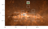 |
Fig. 1 GNS survey fields overlaid on a Spitzer/IRAC color mosaic (3.6,4.5, and 8 μm; Stolovy et al. 2006). Solid white lines indicate the full extent of the GNS. White shaded regions mark the fields analyzed in this work, while dotted and dashed outlines denote the fields of view of the GNS I and GNS II pointings, respectively. The black numbers label the individual fields (see Table 1). Green and blue areas indicate the regions where we computed PMs. The green area corresponds to a field on the Galactic bar, and the solid blue box corresponds to the GNS fields that overlap with the Arches cluster. The black box shows the coverage of the catalog from Hosek et al. (2022). |
2 Observations
The GNS I observations were obtained mostly in 2015, with additional observations in 2016 and 2017, with the wide-field near-infrared camera HAWK-I/VLT in fast-photometry mode. The data were reduced using the speckle holography algorithm (Schödel et al. 2013), achieving a homogeneous angular resolution of 0.2″ (Nogueras-Lara et al. 2018). The survey covers an area of ~ 6000 pc2 (Fig. 1). Due to the extreme crowding in the GC, the sky background was estimated using dithered exposures of a dark cloud near the GC (α ≈ 17h48m01.55s, δ ≈ -28°59′20″), where the stellar density is very low. For further details on these observations, we refer the reader to Nogueras-Lara et al. (2019). Specifically, GNSIDR1 provides photometry for ~3.3 × 10⁶ stars in the J, H, and Ks bands, with typical uncertainties of ≲0.05 mag in all three bands.
The observations for GNS II were acquired in 2022 with a general observing strategy similar to the one used in GNS I. There are, however, two key differences between the two epochs. The first concerns the detector size. In GNS I, the fastphotometry mode was employed with a Detector Integration Time (DIT) of 1.26 s, which restricted the usable area to one-third of the detector (2048 × 768 pixels). In GNS II, with a DIT of 3.32 s, we were able to use the full detector array (2048 × 2048 pixels), thus allowing us to image three times larger areas with a single pointing. The second major difference is the use of the GRAAL ground layer adaptive optics system (Paufique et al. 2010) in GNS II. We increased the DIT and used the full detector window to enable the use of the GRAAL adaptive optics system, thereby improving point spread function (PSF) stability across the field.
In this pilot study, we have reduced and analyzed two fields for GNS I and two for GNS II. Details of these fields are shown in Table 1. The dotted and dashed boxes in Fig. 1 represent the fields from GNS I and GNS II, respectively.
Observing detail of the fields reduced for this study.
3 Data reduction and analysis
3.1 Data reduction pipeline
In this section, we describe our data reduction procedures up to the point of speckle holography. We highlight similarities and differences with GNSIDR1. We processed the data from each of HAWK-I’s four detector chips separately.
Bad pixel correction, flat-fielding, and sky subtraction were carried out as in GNSIDR1 (Nogueras-Lara et al. 2019). In contrast to GNS I DR1, we used the median of the pixels in the lowest 5% range of values of each dark subtracted science frame to scale the normalized sky before its subtraction. It was 10% in case of DR1. This largely avoids negative pixels in the reduced science frames.
Deselection of bad frames was performed. Sometimes the telescope moved during the exposures, resulting in images with smeared or duplicated stars. We rejected those images. On the adaptive optics data (GNS II), we used the MaxiTrack tool (Paillassa et al. 2020), a convolutional neural network designed to automatically identify tracking and guiding errors in astronomical images. This tool does not work well on the older speckle data (GNS I), for which we identified the bad frames by eye.
Geometric distortion correction and precise relative alignment of all short exposures was undertaken (described in detail in the next section). Geometric distortion correction was done with respect to a VVV image in GNSIDR1. For DR2 we used the SCAMP and SWarp software packages from the Astromatic site (Bertin et al. 2002; Bertin 2006). The SExtractor package was used to support these programmes (Bertin & Arnouts 1996). This procedure represents a significant change compared to DR1, and this step has proven to be essential to reaching the high astrometric accuracy of GNS IDR2 and GNS II.
Creation of a long exposure image with its corresponding noise image from the mean and error of the mean of the individual short exposures was realized. The StarFinder package (Diolaiti et al. 2000) was used to extract stars and their photo-astrometry from the long-exposure to use them in the holographic image reconstruction (see below and Schödel et al. 2013; Nogueras-Lara et al. 2018).
Image cubes for 1 × 1 arcmin2 subregions were created as in GNS IDR1. The subregions overlap by 0.5′ on each side, except at the edges of the field of view. The cubes contain all individual short exposures (of length DIT) corresponding to this region.
Speckle holography reduction of the subregions was performed. Different than in GNS I DR1, where three subimages were created from disjunct data, we built a deep image using all frames and also created ten jackknife sampled images, each of which left out a different 10% of the frames. The advantage here is that we can obtain deeper photometry (see Fig. 2) while maintaining reliable noise estimates. As in DR1, we resampled all exposures by a factor of two, using cubic interpolation. A Gaussian beam of 0.2” FWHM was used for beam restoration in the speckle holography algorithm. This resulted in final images with an excellent sharpness and homogenous Gaussian PSFs. In the following, we refer to the reconstructed 1′ × 1′ images as sub-images.
3.2 Geometric distortion correction
We used SCAMP (Bertin 2006) to correct for geometric distortion and to compute the global astrometric solution. We only provide a brief description of the algorithm here. The interested reader can find more details about how SCAMP works in Bouy et al. (2013).
SCAMP is fed with position lists extracted from each exposure with SExtractor (Bertin & Arnouts 1996). It computes the global geometric solution by minimizing the squared positional differences between overlapping sources ( ) in pairs of catalogs:
 (1)
(1)
where s indexes the matched sources, while a and b denote different images. The quantity xs,a represents the observed position of source s in catalog a, typically in pixel coordinates. The function ξa (xs,a) is the transformation that maps these coordinates into a common astrometric reference frame using the current calibration parameters for catalog a. The terms σs,a and σs,b denote the positional uncertainties associated with source s in catalogs a and b.
We show in Fig. 3 an example of the distortion pattern determined by SCAMP for the HAWK-I camera from a GNS II pointing. The color variations in the image represent the deviations of the local pixel scale from the nominal one.
Based on the position catalogs derived from each image, SCAMP generates updated headers for each exposure that encode the geometric distortion solution. These corrected headers were then applied to the images, which were subsequently re-projected onto a common grid using SWarp (Bertin et al. 2002). After processing with SWarp, all exposures shared a consistent astrometric solution and were resampled onto a common, distortion-corrected reference frame.
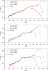 |
Fig. 2 Comparison of the J, H, and Ks luminosity functions for the Galactic bar field (green box in Fig. 1) using data from the VVV catalog by Griggio et al. (2024, available only for the J and Ks bands), from GNSI (DR1 and DR2), and GNSII. |
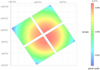 |
Fig. 3 Example of the HAWK-I mosaic camera distortion map provided by SCAMP for a GNS II pointing. Colors encode the variation of the pixel scale across the detector. |
3.3 Photometry and astrometry
Subsequently, we performed point source fitting on the holographically reconstructed images of the 1 × 1 arcmin2 subregions and created lists and images for the full field of view of each pointing. The following steps describe in detail the procedure applied to derive these products.
The PSF of each sub-image was extracted with an automatic script based on StarFinder that builds a median PSF from 5 to 40 unsaturated bright and isolated stars (any star within 0.4”, about the FWHM of the PSF of a reference star, must be at least five magnitudes fainter; the exact numbers can be varied without any significant impact on the results). The PSF was extracted iteratively to take into account secondary sources near the reference stars. Five stars is the minimum necessary for a good PSF determination (and to minimize bias due to individual stars). While about 20 reference stars will provide a very good estimate of the PSF, up to 40 are used in case a field is extremely crowded or contains only faint stars. The exact number can be varied and does not have any significant influence on the results.
The positions and fluxes of the stars were measured with StarFinder with two iterations using relative thresholds of 3 σ and a minimum correlation value of 0.7. Extended emission may be present in the images due to unresolved stellar sources or diffuse emission from ionized gas. This extended emission was subtracted by StarFinder before making the measurements. The extended emission was estimated by StarFinder on 2.4” × 2.4” regions and then interpolated across the field. We chose this region because it is large enough to obtain reasonably accurate estimates of the diffuse emission in the crowded GC. This choice does not have any strong influence on the results because StarFinder will always fit a slanted background when fitting the core of any star with the PSF.
The measurement process was carried out on the deep image and its corresponding jackknife sampled images. The resulting point source lists were then combined. A source is considered real only if it is detected in the deep image and in all jackknife images. The uncertainties were determined according to standard jackknife statistics: The uncertainty of njack samples, xi, with mean x̄ is
 .
.The median astrometric and photometric offsets between the source lists of pairwise overlapping sub-images were determined from all sources brighter than 17 mag (all bands) that coincide within 0.1” and that are located at least 1” from the sub-image edges (to avoid potential edge effects), typically between 100-200 sources. These offsets can be related to small variations of the estimated PSFs between the sub-images.
The best astrometric and photometric offsets for each subimage and their corresponding source lists (sub-lists) were estimated with a global optimization algorithm that minimizes the mean square deviations between the pairwise overlapping subregions. This procedure is basically the one that is described in Appendix A of Dong et al. (2011) and represents a major difference from GNSIDR1, where all measurements were related to a single subregion and not globally optimized. This global optimization is another key tool to achieving the high photometric and astrometric accuracy of GNS I DR2 and GNS II.
The astrometric offsets determined in the previous step were applied to the sub-images and their sub-lists to reconstruct a large image and source list for each chip. At this point the pipeline provides two kinds of uncertainties: (1) statistical uncertainties from the jackknife sampling and (2) uncertainties due to variations between the sub-images that can be estimated from the two to four measurements for sources in the overlap regions caused by, for example, uncertainties in the PSF extraction. This second uncertainty is assumed to be the same for all stars. We determined the median of the latter uncertainties for bright (J < 17, H < 16, Ks < 16), unsaturated stars and added it in quadrature to the jackknife uncertainties to take into account the systematics for all sources. Thus, we introduced a floor uncertainty for all sources, ranging from 0.5-1.5 mas in position and 0.02-0.05 mag in photometry.
Astrometric calibration was done with recently published high-precision measurements of the VVV survey toward the GC (Griggio et al. 2024).
Photometric calibration was based on the SIRIUS/IRSF survey (Nagayama et al. 2003; Nishiyama et al. 2006), as in GNS IDR1. We chose the reference stars to be bright, unsaturated, and isolated (any other star within a 2” radius must be at least 5 mag fainter). We obtained about 100 (GNS I) to 300 (GNS II) stars per chip for photometric calibration, which established the zero point with respect to the SIRIUS/IRS survey with (sub)percent precision.
Finally, any astrometric and photometric offsets between the four detector chips were corrected by computing pairwise mean offsets and finding the optimal offset for each chip with a minimization routine, in the same way as we did for the subregions. To avoid any bias introduced by this step, we re-calibrated the photometry with SIRIUS (see previous step). The astrometry of the final lists was calibrated with respect to Gaia DR3 sources within the field by applying simple shifts in Galactic latitude and longitude.
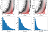 |
Fig. 4 Astrometric and photometric uncertainties of the stars in the Galactic bar field (green box in Fig. 1) using data from GNS IDR2. Upper row: Two-dimensional histograms showing (in gray) the uncertainties estimated by the pipeline for stars of a given magnitude, combining both jackknife and PSF-based uncertainty components. The red dots show the uncertainties of stars as estimated from their multiple detections on different detector chips. Lower row: Histograms of the astrometric and photometric uncertainties of bright (H ≤ 18 [mag]) stars measured on different detectors. |
4 Astrometric and photometric performance
The pipeline determines relative astrometric and photometric uncertainties in two ways: (1) from the uncertainties estimated by jackknife sampling and (2) from the uncertainties estimated from multiple measurements of stars in overlapping parts of the subimages. We refer to the latter uncertainties as PSF uncertainties because they are probably mostly limited by the precision with which the PSF can be estimated for each sub-image, but other sources of uncertainty, such as uncertainties of the flat field, play a role, too. The PSF uncertainties provide a lower floor to all measurements. We therefore added them in quadrature to the jackknife uncertainties.
Due to the dithering of the observations, a large number of stars were observed multiple times on different detector chips. These independent measurements can be used to cross-check the robustness of the uncertainties estimated by our pipeline. Figure 4 shows a summary plot comparing the uncertainties estimated by the pipeline with those derived from repeated measurements across different chips. In the upper panel, the uncertainties estimated by the pipeline (2D histograms) are compared to the uncertainties from multiple measurements on different detectors (red dots). The comparison reveals that our pipeline provides robust, possibly even slightly overestimated, uncertainties. The uncertainties estimated from the independent measurements on different chips may be underestimated at times because there are only two measurements for many stars. We conclude that the uncertainties provided by the pipeline are realistic and give reliable minimum uncertainties at each magnitude.
The lower plot shows histograms of the uncertainties of bright (H ≤ 18 mag) stars detected on different detector chips. We omitted faint stars to minimize the influence of random uncertainties. The histograms show astrometric uncertainties of a few milliarcseconds and photometric uncertainties of a few percent. These results are consistent across the J and Ks bands as well as for the GNS II data.
Figure 5 compares the photometry of GNSIDR2 in the J, H, and Ks bands with that of the SIRIUS survey for all common stars in the field B1. The mean deviations and their uncertainties are 0.010 ± 0.002 mag for the J band, 0.003 ± 0.002 mag for the H band, and 0.001 ± 0.002 mag for the Ks band. This indicates that the uncertainty of the GNS I DR2 photometry is dominated by the 3% systematic zero-point uncertainty of the SIRIUS survey (Nishiyama et al. 2005). As shown in the middle panel of Fig. 5, saturation begins to affect the photometric measurements in GNS I at magnitudes H ≲ 11 (see also Nogueras-Lara et al. 2019). For GNS II, the residuals relative to SIRIUS are fully consistent, with a mean deviation of 0.001 ± 0.002 mag in the H band.
To estimate the astrometric accuracy, we calculated the position residuals in l and b for the H band with respect to Gaia DR3 (Gaia Collaboration 2023) for field B1. Common stars were selected by searching for crossmatches within 0.05″.
Subsequently, a similarity transform was applied to remove a small systematic offset (16.5 mas in l and 3.3 mas in b). As shown in Fig. 6, the residual differences between GNS IDR2 and Gaia DR3 exhibit a standard deviation of less than 4 mas in both l and b. Similar residuals with Gaia DR3 were found when crossmatching with GNS II. Performing the same residual comparison with Gaia DR3 for the same field in GNS I DR1 yielded values of about 20 mas, indicating an improvement by roughly a factor of five with respect to GNS I DR1.
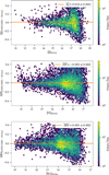 |
Fig. 5 Magnitude residuals between GNS IDR2 and SIRIUS for the J, H, and Ks bands in the Galactic bar field (see Fig. 1). The orange line indicates the mean of the residuals. |
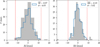 |
Fig. 6 Position residuals in l and b between GNS I DR2 H band stars in the field B1 (Fig. 1) and Gaia DR3 stars in the same field. Blue histograms show the residual distribution after removing the 3σ outliers, while gray histograms show the full distribution before clipping. Dotted red lines indicate the 3σ thresholds. |
5 Proper motions
To compute the PMs, the stellar positions needed to be referenced to a common coordinate system. Although our absolute astrometric uncertainties are already very small, achieving precise PMs required defining a stable reference frame that minimizes the transformation uncertainties between epochs. To this end, we employed two different and independent methodologies to define the reference frame and compute the PMs, which we refer to as relative PMs and absolute PMs. For the PM calculations, we used stars in the H band from each epoch.
5.1 Relative proper motions
In the relative PM method, no absolute reference frame - such as the International Celestial Reference System (ICRS) - is used. Instead, one epoch of the GNS dataset is adopted as the reference epoch, and stellar positions from the other epoch are aligned to this frame. If a sufficiently large number of stars is available, their individual PMs are expected to average out such that the mean motion of the reference population is close to zero. As a consequence, the alignment procedure removes bulk motions common to the reference stars, including large-scale motions associated with Galactic dynamics, and the measured PMs are therefore relative to the mean motion of the reference population. This approach has been widely and successfully applied in studies of the GC (Eckart & Genzel 1997; Ghez et al. 1998; Schödel et al. 2009; Shahzamanian et al. 2022; Martínez-Arranz et al. 2022).
Here we used GNS II as the reference epoch. The results obtained when using GNS I DR2 as the reference epoch are fully compatible. The final product of the data reduction and analysis pipeline is a list of stars for each pointing, which we obtained by combining the four detector chips. Considering the nominal size of the HAWK-I detector and the jittering applied during the observations, each of these lists covers an area of -7.8′ × 3.5′ for GNSIDR2 and ~7.8′ × 7.8′ for GNSII.
We projected the stellar coordinates from both epochs onto the same tangential plane. The GNS IDR2 sources were then aligned with those of GNS II. To select suitable reference stars and ensure uniform sampling, we divided the reference field into a grid of ~2.5 × 2.5 arcsec, thereby avoiding a bias toward regions of higher stellar density. In each cell, we selected a single reference star with 12 < H < 18 mag, choosing the one with the lowest positional uncertainty and ensuring it was isolated within a radius of 1″ from any companion.
We crossmatched the reference catalog with the target epoch, considering a positive match as a source within 50 mas and with an H-band magnitude difference within 3σ. These matches were used exclusively for the fine alignment of the two epochs. A similarity transformation was computed from the matched sources and applied to the entire target catalog. The catalogs were then crossmatched again using the same 50 mas matching radius, and a first-degree polynomial transformation was derived from the new matches and applied to all sources. This procedure was repeated iteratively until the number of matches converged.
Subsequently, the polynomial degree was increased to two, and the iterative alignment procedure, still using a matching distance of 50 mas, was repeated. Little to no improvement was achieved with a third-degree polynomial, so we limited our procedure to a polynomial degree of two. Finally, after the alignment was completed, the positions in the two epochs were crossmatched using an increased matching distance of 150 mas, and the resulting positional offsets were divided by the time baseline to derive the PMs, with standard error propagation applied to estimate the uncertainties.
To estimate the uncertainty of the alignment procedure, we applied a bootstrapping method by randomly resampling (with replacement) the set of reference stars 300 times. The standard deviation of the resulting distributions of the reference star positions was adopted as the estimate of the alignment uncertainty. The top panel of Fig. 7 shows the map of the mean alignment uncertainty as a function of l and b ( ). The alignment uncertainty is well below 2 mas across almost the entire field.
To determine the overall PM uncertainties, we applied standard error propagation by taking into account the individual position uncertainties for each star in the directions parallel and perpendicular to the Galactic plane for each epoch combined with the alignment uncertainty. In Fig. 8 we show the mean PM uncertainty ( ) for the parallel and perpendicular components versus the H magnitude.
Finally, to assess the quality of the relative PMs, we compared our PMs with those measured by Gaia DR3. We identified Gaia stars within our Galactic bar field (green box in Fig. 1) and used their PMs to calculate the expected positions of Gaia stars at the time of our reference epoch. We propagated the uncertainties accordingly. We transformed the PMs to Galactic coordinates μl × cos b and μb. We applied a quality cut to select the most suitable stars for the comparison. (i) We excluded Gaia stars with magnitudes fainter than G = 19 and brighter than 13 to avoid high astrometric uncertainties. (ii) We then discarded Gaia stars with a close Gaia companion to prevent mismatching. (iii) We selected only sources with a five-parameter astrometric solution (position, parallax, and PM). (iv) Finally, we eliminated Gaia sources with negative parallaxes, which are unphysical.
For the GNS catalog, we restricted the comparison to stars with PM uncertainties smaller than 1.5 mas yr−1 and crossmatched them with Gaia stars, considering as a positive match any pair of sources within a 50 mas radius. In the top row of Fig. 9, we show the residuals between Gaia and GNS. After clipping 3 σ outliers, we achieved an rms of ~0.5 mas yr−1. The mean offsets in the PMs parallel and perpendicular to the Galactic plane are due to the fact that we used a relative frame of reference. The relative reference frame assumes that the mean motion of all stars is zero in all directions. The offset with respect to Gaia corresponds to the motion of the Solar System relative to the average motion of the reference star. This motion is 5.4 mas yr−1 (211 km s−1) along the east-west and 0.4 mas yr−1 (15.6 km s−1) in the north-south direction, in agreement within the uncertainties with what has been measured by radio interferometry (e.g., Reid & Brunthaler 2020).
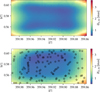 |
Fig. 7 Top: Total relative alignment uncertainties across the green region in Fig. 1. Bottom: Mean absolute alignment uncertainties in the same region, with Gaia reference stars marked in black. |
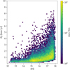 |
Fig. 8 Mean PM uncertainty versus H magnitude from the relative alignment. This plot corresponds to the stars in the green box region in Fig. 1 for stars with magnitudes 12 < H < 18. |
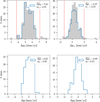 |
Fig. 9 Gaia-GNS PM residuals for the Galactic bar field (green box in Fig. 1). Left panels: residuals of the parallel component. Right panels: residuals of the perpendicular component. Top: residuals of the relative PMs. Bottom: Residuals of the absolute PMs. Gray histograms show the full distribution before clipping, and blue histograms show the same but after removing the 3σ outliers. Dotted red lines indicate the 3σ thresholds. |
5.2 Absolute proper motions
In the absolute method, PMs are defined with respect to an absolute reference frame. We used Gaia stars present in the field to anchor our astrometry and followed the procedure described below.
First, we selected the most suitable set of Gaia reference stars. We relied on stars from Gaia DR3 (Gaia Collaboration 2023), which provides a significant improvement in astrometric precision compared to Gaia DR2 (Gaia Collaboration 2018), reducing the PM uncertainty by a factor of about two (Lindegren et al. 2021).
Due to the high visual extinction toward the GC, the Gaia mission is largely insensitive to its stellar population, resulting in only a very limited number of usable Gaia stars in this region. However, a few foreground stars have well-measured Gaia astrometry and can serve to link the GNS catalog to the ICRS, an approach used in many previous studies (see, e.g., Libralato et al. 2021; Hosek et al. 2022; Griggio et al. 2024). Given the small number of available reference stars, careful selection is critical to avoid poor-quality anchors. To this end, we applied the same quality filters described in the preceding section. The remaining stars after these cuts were adopted as the reference stars.
Next, we used Gaia PMs to propagate their position to the corresponding GNS epochs. Then, we projected Gaia stars and GNS stars to a common tangential plane and crossmatched Gaia stars with their GNS counterparts, considering sources separated by less than 50 mas as positive matches. These matched stars were used to compute similarity transformations, which were applied to the GNS catalogs to place them into the Gaia reference frame. We crossmatched the sources again and refined the alignment by applying a second-degree polynomial transformation. We also tested a first-order polynomial, which left statistically significant positional residuals for many reference stars, and a third-order polynomial, which offered no meaningful advantage over the second-degree one. Therefore, we chose a second-order polynomial as the optimal choice.
Finally, we compared the positions of stars common to the GNS I DR2 and GNS II catalogs and divided their positional offsets by the time baseline to derive PMs. At this stage, we increased the matching distance to 150 mas in order to compute the PMs, and the positional offsets were divided by the time baseline. Matches with H-band magnitude differences greater than 3σ were discarded. The resulting PMs and stellar positions were then compared to Gaia again, and the 3σ outliers were removed from the Gaia reference star list. The process was repeated until no more 3σ outliers remained.
As done previously, we estimated the uncertainty of the alignment of GNS I DR2 and GNS II with the Gaia reference frame with a bootstrapping method. In Fig. 7 (bottom panel), we show the alignment uncertainties. In Fig. 9 (bottom panel) we show the residuals of the absolute PMs with Gaia. As in the case of the relative PMs, we reached an rms of ~0.5 mas yr−1. Both methodologies present similar PM residuals with respect to Gaia, confirming the consistency and robustness of the two approaches.
In the bottom panel of Fig. 7, an almost homogeneous distribution of the alignment error across the field can be observed. However, a slight dependence of the alignment quality on the local Gaia stellar density is also noticeable. As we discuss in the next section, this effect becomes more pronounced in the Arches field (Fig. 10, right panel), where the number of Gaia stars is lower and their spatial distribution is highly heterogeneous. Consequently, alignment uncertainties are larger in regions with fewer available Gaia reference stars. This contrasts with the case of the relative alignment, where the effective density of reference stars is high and largely homogenous across the field, resulting in a more uniform uncertainty distribution.
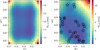 |
Fig. 10 Alignment uncertainty for the solid blue area in Fig. 1. Left: relative alignment. Right: absolute alignment. Black stars mark the position of Gaia reference stars. |
5.3 NSD field
As a secondary test, we analyzed a field containing the Arches cluster (solid blue box in Fig. 1) to assess the quality of the PMs in a highly crowded region, compare the measured PMs to literature values, and study the feasibility of detecting clusters in such an environment. We computed both relative and absolute PMs as described in Sects. 5.1 and 5.2. The alignment uncertainties for the region containing the Arches cluster are shown in Fig. 10. The left panel displays the results for the relative uncertainties, which, as in the case of the test field on the Galactic bar, show mostly homogeneous values. The right panel presents the alignment uncertainties of the absolute method together with the Gaia reference stars. A strong dependence of the uncertainty on the density of Gaia stars in the field is evident. Figure 11 shows the PM residuals for both the relative and absolute measurements.
We also tested the quality of the relative and absolute PMs by comparing them with the catalog of Hosek et al. (2022), hereafter H22. This catalog consists of astro-photometry data, PMs, and magnitudes (F127M and F153M filters) obtained with the WFC3/HST camera in the area of the Arches cluster (black box in Fig. 1). The precision of the H22 PMs reaches ~0.2 mas yr−1 rms when compared to Gaia DR3, and similar to our absolute PMs, the H22 catalog is anchored to the ICRS using Gaia DR3 stars.
For the comparison between the GNS and H22 catalogs, we selected stars with low position uncertainties. That is, for GNS, we selected stars with 12 < H < 18, and for H22, we selected stars with 15 < F153M < 20 (see Fig. 2 in Hosek et al. 2022). In both cases we discarded stars with PM uncertainties larger than 0.5 mas yr−1.
Figure 12 shows the residuals of the comparison between H22 and our relative PMs (top panel), and between H22 and our absolute PMs (bottom panel). We achieved a precision of ~0.4 mas yr−1 rms in both cases. These low and homogeneous residuals across both methodologies further demonstrate the reliability and compatibility of the two methods.
Finally, we applied the cluster-finding algorithm described in Martínez-Arranz et al. (2024a) to both the relative and absolute PM catalogs overlapping with the Arches cluster. This tool is based on the density-based spatial clustering of applications with noise algorithm (DBSCAN; Ester et al. 1996), which identifies overdensities in multidimensional spaces. In this case, we searched for overdensities in a four-dimensional space defined by celestial positions and PMs.
For the relative PMs, we subtracted the mean residuals with respect to Gaia in order to place them in the Gaia reference frame. The analysis was restricted to stars with PM uncertainties below 1.5 mas yr−1. In both cases, we identified a dense comoving group of stars. Figure 13 shows the comoving group detected in the relative and absolute catalogs. In the left column, we display a vector-point diagram of the PMs for each catalog, with the relative catalog at the top and absolute catalog at the bottom. In the right column, we show the star positions from each catalog. The green dots represent the stars labeled as members of the same comoving group by the clustering algorithm.
The members of the comoving groups identified in both catalogs, relative and absolute, overlap with the known extent of the Arches cluster. Both groups exhibit consistent mean velocities, within the uncertainties, as well as coincident spatial distributions. The mean velocities parallel and perpendicular to the Galactic plane agree in both cases with the values reported for the Arches cluster by Hosek et al. (2022, μl* = -2.03 ± 0.025 mas yr−1, μb = -0.30 ± 0.029 mas yr−1) and Libralato et al. (2021, μl* = -3.05 ± 0.17 masyr−1, μ b = -0.16 ± 0.20 mas yr−1). A more detailed analysis of the comoving groups identified in our datasets lies beyond the scope of this paper and will be presented in a forthcoming work (Martínez-Arranz et al., in prep.).
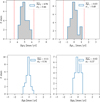 |
Fig. 11 Gaia-GNS PM residuals Arches field in Fig. 1. Top: relative PM residuals Bottom: absolute PM residuals. Gray histograms show the full distribution before clipping. Dotted red lines indicate the 3σ thresholds. |
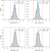 |
Fig. 12 Residuals between H22 and GNS PMs (solid blue field and black square field in Fig. 1). Top: residuals of the relative PMs. Bottom: residuals of the absolute PMs. Gray histograms show the full distribution before clipping. Dotted red lines indicate the 3σ thresholds. |
5.4 Proper motion precision
Precise PM measurements are essential for kinematic studies in the GC. As an illustration, Nieuwmunster et al. (2024) applied a quality cut of σμ < 0.6 mas yr−1 to the PM catalog of Smith et al. (2018) in order to ensure reliable kinematic results. We used this value as a reference to assess the quality of the GNS DR2 PMs by comparing them with those from the VIRAC2 survey (Smith et al. 2025), which currently represents the state of the art in ground-based PM measurements in the GC and is based on VVV and VVVX data covering ~560 deg2 of the southern Galactic plane and bulge.
We repeated an analysis similar to that presented in Sect. 5.2, but comparing VIRAC2 with Gaia. Using Gaia sources overlapping the blue box shown in Fig. 1, we find that VIRAC2 and GNS DR2 achieve comparable residuals with respect to Gaia. However, Gaia detections toward the GC are limited to relatively bright stars. At fainter magnitudes, including the red clump and below, GNS DR2 allows access to a larger and more precise PM sample in the GC region.
This increased depth and precision at fainter magnitudes is illustrated in Fig. 14, where we compare the luminosity functions of GNS DR2 and VIRAC2 for the stars in the NSD field (blue box in Fig. 1) The black and gray histograms show all stars with measured PMs in each catalog, while the blue and orange histograms correspond to stars with PM uncertainties below 0.6 mas yr−1. The approximate location of the red clump is marked in red, based on the color-magnitude diagram (CMD) shown in the bottom panel of Fig. 15. The figure highlights that GNS DR2 retains a substantially larger fraction of high-precision PMs at red-clump and fainter magnitudes.
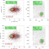 |
Fig. 13 Comoving groups identified in the Arches field (blue box in Fig. 1). Left column: PMs. Right column: positions. Top left: Relative PMs, after subtracting the mean residuals with respect to Gaia. Bottom left: absolute PMs. Green points represent the stars identified by the clustering algorithm as members of a comoving group, red crosses mark stars within 1.5 times the radius of the comoving group, and black points correspond to field stars. The boxes indicate the mean PM values with their dispersions, the approximate radius of the comoving group, the number of identified members, and their mean positions. |
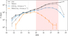 |
Fig. 14 GNS and VIRAC2 H-band luminosity functions for the NSD field (blue box in Fig. 1). The black and gray histograms show the luminosity functions from GNS and VIRAC2, respectively, for all stars with measured PMs. The blue and orange histograms show the luminosity functions after applying a PM uncertainty cut, excluding stars with errors larger than 0.6 mas yr−1. The red shaded region marks the approximate location of the red clump stars. |
6 Kinematic analysis
The interpretation of the NSD as a dynamically distinct component from the bulge has been questioned recently. Zoccali et al. (2024) argue that the nuclear region exhibits clear signatures of rotation in PM space, with the brighter half of red clump stars moving eastward in longitude and the fainter half moving westward. They further identify a confined structure within -1.5 < l < 0.8 and -0.25 < b < +0.1 in which red clump stars predominantly move eastward. This behavior is interpreted as a consequence of the central molecular zone (CMZ) obscuring the far side of the nuclear region. Based on these findings, they did not find compelling evidence for the presence of a cold fast-rotating NSD in the available PM data nor in previously published studies. While they do not rule out its existence, they conclude that the observed kinematic signatures are qualitatively consistent with projection and extinction effects induced by the CMZ rather than requiring a dynamically distinct NSD.
The presence of the CMZ would clearly affect the velocity distribution along the direction of the Galactic plane since most stars on the far side of the nuclear region are obscured. However, the distribution of the perpendicular component is expected to remain homogeneous, as it should be similar on the near and far sides. Consequently, in the absence of a dynamically distinct structure, the PM distribution of the perpendicular component should be the same in the central and northern regions. On the other hand, if the NSD is dynamically colder than the surrounding environment, its PM distribution should differ from that of the bulge, exhibiting a smaller velocity dispersion.
In Fig. 15, we show the CMD and the distributions of the vertical component of the relative PMs for the bulge (top) and NSD (bottom) fields (green and blue boxes, respectively, in Fig. 1). The vertical orange line in the CMD indicates the color cut adopted to remove foreground populations from the PM distributions (Nogueras-Lara et al. 2021b). The boxes in the right-hand panels show the mean PM and its standard deviation. The corresponding uncertainties were estimated using a bootstrap resampling method in which the distributions were resampled with replacement 300 times. The PM dispersion measured for the bulge field (top panel of Fig. 15) is consistent with the dispersion of μb for bulge stars reported by Clarkson et al. (2008). Comparison of the top- and bottom-right panels showed that the PM dispersion of stars in the NSD field is smaller than that measured in the bulge field, indicating different kinematic properties between the two fields.
Assuming that, on average toward the GC, a larger extinction corresponds to a greater distance along the line of sight (see, e.g., Nogueras-Lara 2022a; Martínez-Arranz et al. 2024a), we compared the vertical PM distributions at different depths by applying two distinct color cuts to each distribution. Table 2 lists the color cuts adopted from the CMDs shown in Fig. 15 together with the dispersion of the perpendicular component of the relative PMs for the stars selected within each color range. The widths of these color cuts were adjusted to account for the different degrees of extinction observed in the two fields. Table 2 shows that the parameters of the distributions remain approximately constant within the uncertainties for the different color cuts.
We find that the dispersion of the vertical component of the PMs for stars analyzed in both fields, after removing the foreground population, is smaller for the NSD population than for the bulge. Moreover, this difference is preserved for stellar populations located at different depths. This behavior suggests that the population associated with the NSD region belongs to a dynamically distinct, colder structure. This interpretation is consistent with the dynamics of nuclear disks or rings observed in other spiral galaxies, which exhibit smaller velocity dispersions than the surrounding medium (see, e.g., Gadotti et al. 2019).
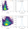 |
Fig. 15 CMD and distributions of the vertical component for relative PMs for the bulge (top) and NSD (bottom) fields corresponding to the green and blue boxes in Fig. 1. The vertical orange line in the CMD indicates the color cut applied to remove the foreground. The red box in the CMD in the bottom panel marks the approximate position of the red clump stars. |
7 Conclusions
We have described the updated methodology applied to produce the second data release (DR2) of the GNS survey. Notably, DR2 builds on the first epoch of JHKs imaging presented by Nogueras-Lara et al. (2019). In addition, we include the H-band observations from a second epoch of GNS imaging. In this work, we focused on detailing the new reduction, calibration, and analysis procedures, and we demonstrated their performance using two representative test fields. The full catalog will be released in a future publication.
The updated data reduction and analysis methods allowed us to reach absolute astrometry of 5 mas, an improvement by a factor of about ten compared to GNS I DR 1. The photometric uncertainties are generally less than 5% in all bands. Their basic limitation is the approximately 3% zero point uncertainty of the SIRIUS/IRSF GC survey, which we used for photometric calibration (Nagayama et al. 2003; Nishiyama et al. 2006). Finally, GNS I DR 2 is about 0.5 mag deeper than DR 1, which is mostly due to the adoption of a jackknife algorithm to estimate the uncertainties.
We have presented the methodology and performance of the first PM measurements based on two epochs of GNS H-band imaging. Despite relying solely on ground-based observations and only two epochs separated by seven years (six in the case of the fields B1 and 20) , the PMs we obtained achieve a precision comparable to that from space-based multi-epoch data. We implemented and compared two independent methods to define the reference frame and obtained consistent results. This dual approach provides the flexibility to select the most suitable methodology depending on the characteristics of each field, such as stellar density, extinction, or the availability of Gaia reference stars. We note that as a consequence of using a two-epoch PM calculation, parallactic motion is not explicitly included. However, given the distance to the GC of 8.2 kpc and that the observations were mostly obtained during the same fourth month of the year, the effect on the measured PMs is negligible, well below ~0.1 mas yr−1 for all but the nearest stars.
We have demonstrated that alignment with the Gaia reference frame is not always optimal because this strongly depends on the availability and spatial distribution of Gaia stars in a given field. In some cases, relative PMs provide a robust alternative. Conversely, in regions of very high extinction where relative alignment becomes less effective, the absolute method based on Gaia stars can still be applied successfully.
Our PM achieves an accuracy comparable to that of spacebased studies. This confirms that the technique can be further extended by incorporating data from space-based telescopes such as JWST or the future Roman Space Telescope. Such extensions will allow us to significantly improve the current ~0.5 mas yr−1 accuracy (rms with comparison to Gaia) that we can achieve.
Two of the test files we reduced overlap with the Arches cluster. The clustering algorithm described by Martínez-Arranz et al. (2024a) successfully identified the Arches cluster, with mean velocity components consistent with previous studies based on fundamentally different datasets and methodologies (Hosek et al. 2022; Libralato et al. 2020). This highlights the effectiveness of our approach for detecting and characterizing stellar clusters in the crowded and complex environment of the GC.
By analyzing the dispersion of the vertical component of the relative PMs in the bulge and NSD fields, we find that the NSD exhibits a systematically smaller velocity dispersion than the bulge. This difference persists for stellar population samples at different depths along the line of sight. These results support the interpretation of the NSD as a dynamically colder and distinct structure within the GC, in agreement with the kinematic properties of nuclear disks or rings observed in other spiral galaxies.
As demonstrated by Martínez-Arranz et al. (2024a) and Martínez-Arranz et al. (2024b) for the case of the Candela 1 cluster, the future GNS PM catalog will enable us to search for and characterize so far unknown stellar associations and streams in regions suspected to host recent star formation, such as Sgr B1 and Sgr C (see Fig. 1), where recent studies point to the presence of ~105 M⊙ of newly formed stars (Nogueras-Lara et al. 2022; Nogueras-Lara 2024). This opens the possibility of studying the kinematics of the youngest stellar populations in the NSD, thereby addressing questions such as the missing cluster problem or testing whether the initial mass function is fundamentally different in this extreme environment compared to the Galactic disk, as some studies have suggested (Morris 1993; Bartko et al. 2010; Hosek et al. 2019). The GNS PM catalog will also provide us with a new tool to understand the structure and formation history of the NSD. Work is currently underway on the data release of these catalogs, which will make such studies possible in the near future.
Acknowledgements
AMA, RS, and FNL acknowledge financial support from the project ref. AST22_00001_12 with funding from the European Union -NextGenerationEU, the Ministry of Science, Innovation and Universities (Spain), the Recovery, Transformation and Resilience Plan, the Regional Ministry of University, Research and Innovation of the Government of Andalusia, and the Spanish National Research Council (CSIC), and by the Severo Ochoa grant CEX2021-001131-S funded by MCIN/AEI/10.13039/501100011033 and from grant PID2022-136640NB-C21 funded by MCIN/AEI/10.13039/501100011033 and by the European Union, as well as support from grant PID2024-162148NA-I00, funded by MCIN/AEI/10.13039/501100011033 and the European Regional Development Fund (ERDF) “A way of making Europe”. FNL acknowledges financial support from the Ramón y Cajal programme (RYC2023-044924-I) funded by MCIN/AEI/10.13039/501100011033 and FSE+.
References
- Bartko, H., Martins, F., Trippe, S., et al. 2010, ApJ, 708, 834 [Google Scholar]
- Bertin, E. 2006, in Astronomical Society of the Pacific Conference Series, 351, Astronomical Data Analysis Software and Systems XV, eds. C. Gabriel, C. Arviset, D. Ponz, & S. Enrique, 112 [Google Scholar]
- Bertin, E., & Arnouts, S. 1996, A&AS, 117, 393 [Google Scholar]
- Bertin, E., Mellier, Y., Radovich, M., et al. 2002, in Astronomical Society of the Pacific Conference Series, 281, Astronomical DataAnalysis Software and Systems XI, eds. D. A. Bohlender, D. Durand, & T. H. Handley, 228 [Google Scholar]
- Bouy, H., Bertin, E., Moraux, E., et al. 2013, A&A, 554, A101 [NASA ADS] [CrossRef] [EDP Sciences] [Google Scholar]
- Clarkson, W., Sahu, K., Anderson, J., et al. 2008, ApJ, 684, 1110 [NASA ADS] [CrossRef] [Google Scholar]
- Diolaiti, E., Bendinelli, O., Bonaccini, D., et al. 2000, SPIE Conf. Ser., 4007, 879 [Google Scholar]
- Dong, H., Wang, Q. D., Cotera, A., et al. 2011, MNRAS, 417, 114 [Google Scholar]
- Eckart, A., & Genzel, R. 1997, MNRAS, 284, 576 [NASA ADS] [Google Scholar]
- Ester, M., Kriegel, H.-P., Sander, J., & Xu, X. 1996, in Second International Conference on Knowledge Discovery and Data Mining (KDD’96), Proceedings of a conference held August 2-4, eds. D. W. Pfitzner, & J. K. Salmon, 226 [Google Scholar]
- Gadotti, D. A., Sánchez-Blázquez, P., Falcón-Barroso, J., et al. 2019, MNRAS, 482, 506 [Google Scholar]
- Gaia Collaboration (Brown, A. G. A., et al.) 2018, A&A, 616, A1 [NASA ADS] [CrossRef] [EDP Sciences] [Google Scholar]
- Gaia Collaboration (Vallenari, A., et al.) 2023, A&A, 674, A1 [NASA ADS] [CrossRef] [EDP Sciences] [Google Scholar]
- Gaia Collaboration (Panuzzo, P., et al.) 2024, A&A, 686, L2 [NASA ADS] [CrossRef] [EDP Sciences] [Google Scholar]
- Ghez, A. M., Klein, B. L., Morris, M., & Becklin, E. E. 1998, ApJ, 509, 678 [NASA ADS] [CrossRef] [Google Scholar]
- Griggio, M., Libralato, M., Bellini, A., et al. 2024, A&A, 687, A94 [NASA ADS] [CrossRef] [EDP Sciences] [Google Scholar]
- Hosek, Matthew W. J., Lu, J. R., Anderson, J., et al. 2019, ApJ, 870, 44 [NASA ADS] [CrossRef] [Google Scholar]
- Hosek, M. W., Do, T., Lu, J. R., et al. 2022, ApJ, 939, 68 [NASA ADS] [CrossRef] [Google Scholar]
- Libralato, M., Fardal, M., Lennon, D., van der Marel, R. P., & Bellini, A. 2020, MNRAS, 497, 4733 [NASA ADS] [CrossRef] [Google Scholar]
- Libralato, M., Lennon, D. J., Bellini, A., et al. 2021, MNRAS, 500, 3213 [Google Scholar]
- Lindegren, L., Klioner, S. A., Hernández, J., et al. 2021, A&A, 649, A2 [EDP Sciences] [Google Scholar]
- Martínez-Arranz, Á., Schödel, R., Nogueras-Lara, F., & Shahzamanian, B. 2022, A&A, 660, L3 [NASA ADS] [CrossRef] [EDP Sciences] [Google Scholar]
- Martínez-Arranz, Á., Schödel, R., Nogueras-Lara, F., Hosek, M. W., & Najarro, F. 2024a, A&A, 683, A3 [NASA ADS] [CrossRef] [EDP Sciences] [Google Scholar]
- Martínez-Arranz, A., Schödel, R., Nogueras-Lara, F., et al. 2024b, A&A, 685, L7 [NASA ADS] [CrossRef] [EDP Sciences] [Google Scholar]
- Minniti, D., Lucas, P. W., Emerson, J. P., et al. 2010, New A, 15, 433 [Google Scholar]
- Morris, M. 1993, ApJ, 408, 496 [NASA ADS] [CrossRef] [Google Scholar]
- Nagayama, T., Nagashima, C., Nakajima, Y., et al. 2003, Proc. SPIE, 4841, 459 [NASA ADS] [CrossRef] [Google Scholar]
- Nieuwmunster, N., Schultheis, M., Sormani, M., et al. 2024, A&A, 685, A93 [NASA ADS] [CrossRef] [EDP Sciences] [Google Scholar]
- Nishiyama, S., Nagata, T., Baba, D., et al. 2005, ApJ, 621, L105 [NASA ADS] [Google Scholar]
- Nishiyama, S., Nagata, T., Sato, S., et al. 2006, ApJ, 647, 1093 [NASA ADS] [CrossRef] [Google Scholar]
- Nogueras-Lara, F. 2022a, A&A, 668, L8 [NASA ADS] [CrossRef] [EDP Sciences] [Google Scholar]
- Nogueras-Lara, F. 2022b, A&A, 666, A72 [NASA ADS] [CrossRef] [EDP Sciences] [Google Scholar]
- Nogueras-Lara, F. 2024, A&A, 681, L21 [NASA ADS] [CrossRef] [EDP Sciences] [Google Scholar]
- Nogueras-Lara, F., Gallego-Calvente, A. T., Dong, H., et al. 2018, A&A, 610, A83 [NASA ADS] [CrossRef] [EDP Sciences] [Google Scholar]
- Nogueras-Lara, F., Schödel, R., Gallego-Calvente, A. T., et al. 2019, A&A, 631, A20 [NASA ADS] [CrossRef] [EDP Sciences] [Google Scholar]
- Nogueras-Lara, F., Schödel, R., Gallego-Calvente, A. T., et al. 2020a, Nat. Astron., 4, 377 [Google Scholar]
- Nogueras-Lara, F., Schödel, R., Neumayer, N., et al. 2020b, A&A, 641, A141 [EDP Sciences] [Google Scholar]
- Nogueras-Lara, F., Schödel, R., & Neumayer, N. 2021a, A&A, 653, A33 [NASA ADS] [CrossRef] [EDP Sciences] [Google Scholar]
- Nogueras-Lara, F., Schödel, R., & Neumayer, N. 2021b, A&A, 653, A133 [NASA ADS] [CrossRef] [EDP Sciences] [Google Scholar]
- Nogueras-Lara, F., Schödel, R., & Neumayer, N. 2021c, ApJ, 920, 97 [NASA ADS] [CrossRef] [Google Scholar]
- Nogueras-Lara, F., Schödel, R., Neumayer, N., & Schultheis, M. 2021d, A&A, 647, L6 [NASA ADS] [CrossRef] [EDP Sciences] [Google Scholar]
- Nogueras-Lara, F., Schödel, R., & Neumayer, N. 2022, Nat. Astron., 6, 1178 [NASA ADS] [CrossRef] [Google Scholar]
- Nogueras-Lara, F., Schultheis, M., Najarro, F., et al. 2023, A&A, 671, L10 [NASA ADS] [CrossRef] [EDP Sciences] [Google Scholar]
- Paillassa, M., Bertin, E., & Bouy, H. 2020, A&A, 634, A48 [NASA ADS] [CrossRef] [EDP Sciences] [Google Scholar]
- Paufique, J., Bruton, A., Glindemann, A., et al. 2010, Proc. SPIE, 7736, 77361P [Google Scholar]
- Reid, M. J., & Brunthaler, A. 2020, ApJ, 892, 39 [Google Scholar]
- Saito, R. K., Minniti, D., Dias, B., et al. 2012, A&A, 544, A147 [NASA ADS] [CrossRef] [EDP Sciences] [Google Scholar]
- Schödel, R., Merritt, D., & Eckart, A. 2009, A&A, 502, 91 [NASA ADS] [CrossRef] [EDP Sciences] [Google Scholar]
- Schödel, R., Yelda, S., Ghez, A., et al. 2013, MNRAS, 429, 1367 [Google Scholar]
- Shahzamanian, B., Schödel, R., Nogueras-Lara, F., et al. 2022, A&A, 662, A11 [NASA ADS] [CrossRef] [EDP Sciences] [Google Scholar]
- Smith, L. C., Lucas, P. W., Kurtev, R., et al. 2018, MNRAS, 474, 1826 [Google Scholar]
- Smith, L. C., Lucas, P. W., Koposov, S. E., et al. 2025, MNRAS, 536, 3707 [NASA ADS] [CrossRef] [Google Scholar]
- Stolovy, S., Ramirez, S., Arendt, R. G., et al. 2006, J. Phys. Conf. Ser., 54, 176 [CrossRef] [Google Scholar]
- Zoccali, M., Rojas-Arriagada, A., Valenti, E., et al. 2024, A&A, 684, A214 [NASA ADS] [CrossRef] [EDP Sciences] [Google Scholar]
All Tables
All Figures
|
Fig. 1 GNS survey fields overlaid on a Spitzer/IRAC color mosaic (3.6,4.5, and 8 μm; Stolovy et al. 2006). Solid white lines indicate the full extent of the GNS. White shaded regions mark the fields analyzed in this work, while dotted and dashed outlines denote the fields of view of the GNS I and GNS II pointings, respectively. The black numbers label the individual fields (see Table 1). Green and blue areas indicate the regions where we computed PMs. The green area corresponds to a field on the Galactic bar, and the solid blue box corresponds to the GNS fields that overlap with the Arches cluster. The black box shows the coverage of the catalog from Hosek et al. (2022). |
| In the text | |
|
Fig. 2 Comparison of the J, H, and Ks luminosity functions for the Galactic bar field (green box in Fig. 1) using data from the VVV catalog by Griggio et al. (2024, available only for the J and Ks bands), from GNSI (DR1 and DR2), and GNSII. |
| In the text | |
|
Fig. 3 Example of the HAWK-I mosaic camera distortion map provided by SCAMP for a GNS II pointing. Colors encode the variation of the pixel scale across the detector. |
| In the text | |
|
Fig. 4 Astrometric and photometric uncertainties of the stars in the Galactic bar field (green box in Fig. 1) using data from GNS IDR2. Upper row: Two-dimensional histograms showing (in gray) the uncertainties estimated by the pipeline for stars of a given magnitude, combining both jackknife and PSF-based uncertainty components. The red dots show the uncertainties of stars as estimated from their multiple detections on different detector chips. Lower row: Histograms of the astrometric and photometric uncertainties of bright (H ≤ 18 [mag]) stars measured on different detectors. |
| In the text | |
|
Fig. 5 Magnitude residuals between GNS IDR2 and SIRIUS for the J, H, and Ks bands in the Galactic bar field (see Fig. 1). The orange line indicates the mean of the residuals. |
| In the text | |
|
Fig. 6 Position residuals in l and b between GNS I DR2 H band stars in the field B1 (Fig. 1) and Gaia DR3 stars in the same field. Blue histograms show the residual distribution after removing the 3σ outliers, while gray histograms show the full distribution before clipping. Dotted red lines indicate the 3σ thresholds. |
| In the text | |
|
Fig. 7 Top: Total relative alignment uncertainties across the green region in Fig. 1. Bottom: Mean absolute alignment uncertainties in the same region, with Gaia reference stars marked in black. |
| In the text | |
|
Fig. 8 Mean PM uncertainty versus H magnitude from the relative alignment. This plot corresponds to the stars in the green box region in Fig. 1 for stars with magnitudes 12 < H < 18. |
| In the text | |
|
Fig. 9 Gaia-GNS PM residuals for the Galactic bar field (green box in Fig. 1). Left panels: residuals of the parallel component. Right panels: residuals of the perpendicular component. Top: residuals of the relative PMs. Bottom: Residuals of the absolute PMs. Gray histograms show the full distribution before clipping, and blue histograms show the same but after removing the 3σ outliers. Dotted red lines indicate the 3σ thresholds. |
| In the text | |
|
Fig. 10 Alignment uncertainty for the solid blue area in Fig. 1. Left: relative alignment. Right: absolute alignment. Black stars mark the position of Gaia reference stars. |
| In the text | |
|
Fig. 11 Gaia-GNS PM residuals Arches field in Fig. 1. Top: relative PM residuals Bottom: absolute PM residuals. Gray histograms show the full distribution before clipping. Dotted red lines indicate the 3σ thresholds. |
| In the text | |
|
Fig. 12 Residuals between H22 and GNS PMs (solid blue field and black square field in Fig. 1). Top: residuals of the relative PMs. Bottom: residuals of the absolute PMs. Gray histograms show the full distribution before clipping. Dotted red lines indicate the 3σ thresholds. |
| In the text | |
|
Fig. 13 Comoving groups identified in the Arches field (blue box in Fig. 1). Left column: PMs. Right column: positions. Top left: Relative PMs, after subtracting the mean residuals with respect to Gaia. Bottom left: absolute PMs. Green points represent the stars identified by the clustering algorithm as members of a comoving group, red crosses mark stars within 1.5 times the radius of the comoving group, and black points correspond to field stars. The boxes indicate the mean PM values with their dispersions, the approximate radius of the comoving group, the number of identified members, and their mean positions. |
| In the text | |
|
Fig. 14 GNS and VIRAC2 H-band luminosity functions for the NSD field (blue box in Fig. 1). The black and gray histograms show the luminosity functions from GNS and VIRAC2, respectively, for all stars with measured PMs. The blue and orange histograms show the luminosity functions after applying a PM uncertainty cut, excluding stars with errors larger than 0.6 mas yr−1. The red shaded region marks the approximate location of the red clump stars. |
| In the text | |
|
Fig. 15 CMD and distributions of the vertical component for relative PMs for the bulge (top) and NSD (bottom) fields corresponding to the green and blue boxes in Fig. 1. The vertical orange line in the CMD indicates the color cut applied to remove the foreground. The red box in the CMD in the bottom panel marks the approximate position of the red clump stars. |
| In the text | |
Current usage metrics show cumulative count of Article Views (full-text article views including HTML views, PDF and ePub downloads, according to the available data) and Abstracts Views on Vision4Press platform.
Data correspond to usage on the plateform after 2015. The current usage metrics is available 48-96 hours after online publication and is updated daily on week days.
Initial download of the metrics may take a while.