| Issue |
A&A
Volume 708, April 2026
|
|
|---|---|---|
| Article Number | A193 | |
| Number of page(s) | 14 | |
| Section | Extragalactic astronomy | |
| DOI | https://doi.org/10.1051/0004-6361/202558306 | |
| Published online | 08 April 2026 | |
The SPHINX public data release
II. Using low-ionisation absorption lines and dust attenuation to predict Lyman continuum escape
1
Kapteyn Astronomical Institute, University of Groningen, PO Box 800, 9700 AV, Groningen, The Netherlands
2
Centre de Recherche Astrophysique de Lyon UMR5574, Univ Lyon1, ENS de Lyon, CNRS, F-69230 Saint-Genis-Laval, France
3
Observatoire de Genève, Université de Genève, Chemin Pegasi 51, 1290 Versoix, Switzerland
4
Aix Marseille Univ., CNRS, CNES, Laboratoire d’Astrophysique de Marseille, F-13388 Marseille, France
5
Department of Astronomy, The University of Texas at Austin, 2515 Speedway, Stop C1400 Austin, TX 78712, USA
6
Cosmic Frontier Center, The University of Texas at Austin, Austin, TX 78712, USA
7
Department of Astronomy, Oskar Klein Centre, Stockholm University, 106 91 Stockholm, Sweden
8
LUX, Observatoire de Paris, Université PSL, Sorbonne Université, CNRS, 75014 Paris, France
9
Department of Astronomy, Yonsei University, 50 Yonsei-ro, Seodaemun-gu, Seoul 03722, Republic of Korea
10
Observatoire Astronomique de Strasbourg, Université de Strasbourg, CNRS UMR 7550, 11 rue de l’Université, 67000 Strasbourg, France
11
Department of Astrophysical Sciences, Princeton University, Peyton Hall, Princeton, NJ 08544, USA
★ Corresponding author: This email address is being protected from spambots. You need JavaScript enabled to view it.
Received:
28
November
2025
Accepted:
4
March
2026
Abstract
Context. Low-ionisation state (LIS) metal absorption lines, such as Si II λ1526, are widely used to trace the properties and dynamics of the interstellar medium (ISM) in galaxies. These lines provide crucial insights into galaxy evolution, including feedback mechanisms, metal enrichment, and the escape fraction of ionising photons (fesc) during the epoch of reionisation.
Aims. We expand our understanding of LIS absorption lines as diagnostic tools for ISM properties and fesc. Using the high-resolution SPHINX20 cosmological radiation-hydrodynamics simulation, we generated a comprehensive synthetic dataset of LIS absorption lines and tested their predictive power for fesc in star-forming galaxies.
Methods. Synthetic ISM absorption lines, focusing on Si II λ1260 and Si II λ1526, were computed with the radiative transfer code RASCAS, incorporating resonant scattering of photons, fluorescent emission, and interactions with dust grains. The simulated data enhance the public SPHINX20 dataset with high-resolution LIS lines for the full 1380 galaxies and ten viewing angles per galaxy. We analysed correlations between line properties (width, depth, and Doppler shift), dust attenuation, and fesc, extending previous single-galaxy studies to a statistically significant mock galaxy sample. We also tested our predictions on observed data using the LzLCS and CLASSY surveys.
Results. We found a strong correlation between the dust-corrected residual flux of Si II λ1526, R∼ ≡ Rflux1526 · 10−0.4A1500, and fesc. More precisely, we found fesc ≈ 1.041R∼1.887−0.002, with an average absolute error of 0.02. When we applied observational conditions, the error increased, but the escape fraction was still well recovered. In particular, the measurement of residual fluxes required a very high spectral resolution, and the dust attenuation is not directly observable. We show by applying common tools for fitting the spectral energy distribution to our mock data that the inferred dust attenuation is often far from the correct value, with a tendency to underestimate the attenuation when the effect of dust is strongest.
Conclusions. Our results demonstrate that the residual flux of Si II λ1526 is a powerful predictor of the escape fraction of ionising photons when it is corrected for dust. The spectra, line measurements, and escape fraction values used in this work are made publicly available.
Key words: line: profiles / radiative transfer / dust / extinction / galaxies: high-redshift / dark ages / reionization / first stars
© The Authors 2026
 Open Access article, published by EDP Sciences, under the terms of the Creative Commons Attribution License (https://creativecommons.org/licenses/by/4.0), which permits unrestricted use, distribution, and reproduction in any medium, provided the original work is properly cited.
This article is published in open access under the Subscribe to Open model. This email address is being protected from spambots. You need JavaScript enabled to view it. to support open access publication.
1. Introduction
The interstellar medium (ISM) in star-forming galaxies is a dynamic environment shaped by diverse processes, including star formation, stellar feedback, galactic winds, and gas accretion. Understanding the factors driving its evolution over time is critical for refining our models of galaxy formation and evolution. Observationally, this requires accurate methods for inferring the properties of the ISM. In this context, low-ionisation states (LIS) of metals, such as C+ or Si+, can serve as powerful tracers of neutral and low-ionisation ISM. When seen in absorption against the stellar continuum of galaxies (a so-called down-the-barrel observation), the widths, depth, asymmetry, shifts, and overall complexity of lines such as C II λ1334 or Si II λ1260 encode geometric and dynamic information about the ISM (e.g. Steidel et al. 2010).
The LIS absorption lines are relevant for measuring outflow velocities and inferring mass outflow rates, as has been shown, for example, in Shapley et al. (2003), Heckman et al. (2015), Xu et al. (2023). They were also used to study the metal enrichment of the ISM (see, e.g. James et al. 2014; Chisholm et al. 2018; James & Aloisi 2018). Above all, LIS lines were used in the context of reionisation as a tracer of the escape fraction of ionising photons (fesc). This crucial property of galaxies shows to which extent they contribute to ionising their surrounding intergalactic medium (IGM). Over the past two decades, several ground-breaking detections of Lyman-continuum (LyC) leakage have been achieved in galaxies at low and intermediate redshifts, providing key insights into how ionising photons escape from their ISM (e.g. Bergvall et al. 2006; Vanzella et al. 2010, 2015, 2018; Leitet et al. 2013; Borthakur et al. 2014; Izotov et al. 2016a,b, 2018, 2021; Leitherer et al. 2016; Puschnig et al. 2017; Wang et al. 2019; Flury et al. 2022a; Marques-Chaves et al. 2022; Rivera-Thorsen et al. 2022; Saxena et al. 2022). To understand the reionisation era, it is essential to perform similar measurements at higher redshifts, but this is prevented by the increasing opacity of the IGM to ionising radiation (e.g. Fan et al. 2006; Ouchi et al. 2018; Wise 2019). Consequently, indirect tracers of LyC escape are required. Among these, LIS absorption lines have long appeared as promising diagnostics, since their strength and residual flux directly probe the distribution and covering fraction of neutral gas along the line of sight (LOS) (e.g. Heckman et al. 2011; Erb 2015; Chisholm et al. 2018; Gazagnes et al. 2018; Steidel et al. 2018). Recently, the advent of large spectroscopic surveys such as the Low-z Lyman Continuum Survey (LzLCS: Flury et al. 2022a,b) has enabled statistical studies of these relations, revealing robust connections between fesc and the depth or residual flux of LIS lines (Saldana-Lopez et al. 2022).
These empirical relations have motivated efforts to interpret the LIS line properties in terms of the physical conditions of the ISM and the mechanisms regulating LyC escape. Different modelling approaches have been explored to extract galaxy properties from observed LIS absorption lines. The picket-fence model (e.g. Reddy et al. 2016; Chisholm et al. 2018; Gazagnes et al. 2018; Saldana-Lopez et al. 2023) assumes that a fraction of stars is covered by optically thick gas, while the remaining stars face empty channels, or holes. In this model, the residual flux (i.e. the flux at the bottom of the line over the continuum flux) can be directly linked to fesc. More sophisticated approaches have explored LIS line transfer in moving media and spherical anisotropic geometries using the Sobolev approximation or Monte Carlo simulations (e.g. Prochaska et al. 2011; Scarlata & Panagia 2015; Carr et al. 2018; Garel et al. 2024). While restricted to idealised geometries, these models are able to predict the effects of line infilling since they take multiple scatterings into account. However, it is unclear whether the assumptions made by these models lead to an accurate representation of reality that can be used to infer physical properties of the ISM. In particular, they assume a unique central source, ignore absorption from the fine-structure level (Mauerhofer et al. 2021; Gazagnes et al. 2023), do not account for the Doppler effects emerging from the complex dynamics of gas, ignore the effect of satellite galaxies within the LOS, and oversimplify the complex star-gas-dust geometry (including the precise ionisation state of the gas and over-abundance of dust in cold dense regions).
This gap hampers our ability to interpret the LIS lines quantitatively and to use them as robust diagnostics of the escape of ionising radiation. A self-consistent dataset of simulated absorption spectra, tied to well-defined galaxy properties, is therefore crucial. To address this issue, we took advantage of the rich ensemble of high-redshift star-forming galaxies present in the SPHINX20 simulation (Rosdahl et al. 2022), which is a high-resolution cosmological radiation-hydrodynamics simulation that follows the evolution of tens of thousands of galaxies down to z = 4.64. We enhance the public dataset of the SPHINX20 simulation (Katz et al. 2023) by including high-resolution synthetic ISM absorption lines, focusing on Si II λ1260 and Si II λ1526. We chose these lines because they are among the strongest low-ionisation transitions and remain observable at high redshift, unlike lines shortward of Lyman-α such as O I λ1039 or Si II λλ1190, 1193. While other redder lines such as O I λ1302 or C II λ1334 are also strong, the presence of nearby fluorescent emission or of other absorption lines complicates the interpretation. With the chosen lines, we built a catalogue of realistic LIS absorption lines, which can then be associated with non-observable galaxy properties based on the plethora of data already presented in the data release (Katz et al. 2023). This can be used as tests for current and future models of Si II absorption (and fluorescent) lines, and also for a direct comparison to observations of star-forming galaxies (as in e.g. Gazagnes et al. 2023, 2024).
As an example application of our catalogue of lines, we extend the work of Mauerhofer et al. (2021, hereafter, M21), where we found a correlation between the residual flux of LIS lines, the dust attenuation, and fesc in a single galaxy taken from a SPHINX-like cosmological zoom simulation at different times (from z = 3.2 to z = 3) and viewing angles. Given the importance of identifying reliable indirect tracers of LyC escape, we test here whether these relations persist across a broader population of simulated galaxies and if they might thus be applied to high-redshift observations. We also discuss the obstacles when our predictions are applied on real data, and we test it with observed low-redshift star-forming galaxies using LzLCS and the COS Legacy Archive Spectroscopy Survey (CLASSY: Berg et al. 2022; James et al. 2022).
The paper is structured as follows. In Section 2 we detail the simulation and our modelling techniques. In Section 3 we show how well we can predict fesc using the line properties of Si II λ1526 and the values of the UV dust attenuation. In Section 4 we discuss the limitations of our escape fraction predictions, in particular, we test how accurately the dust attenuation can be estimated via Spectral Energy Distribution (SED) fitting. We also compare our results with observations. Finally, we summarise our findings in Section 5.
2. Simulation and methods
In this section, we describe the new data, which we are making public. We then explain our procedure to generate mock absorption lines.
2.1. Set of simulated galaxies
We analysed virtual galaxies from the radiation-hydrodynamics simulation SPHINX20, presented in Rosdahl et al. (2022). SPHINX20 is a cubic volume of (20 cMpc)3 simulated using the RAMSES-RT adaptive mesh refinement code (Teyssier 2002; Rosdahl et al. 2013). It resolves haloes down to the atomic cooling mass of 3 × 10⁷ M⊙, as a result of its dark matter particle mass of 2.5 × 10⁵ M⊙. The code includes on-the-fly radiative transfer (RT) in two bins of hydrogen-ionising photons using the M1 method (Rosdahl et al. 2013). This volume was selected as the most representative of 60 cosmological initial conditions in order to obtain an average reionisation history. The gas resolution reaches 10 pc in the densest regions of the ISM, which is crucial to resolve the escape of ionising radiation and the photochemistry of interstellar gas. In star formation, gas is converted into stars in cells with a gas density higher than 10 cm−3, a locally turbulent Jeans length smaller than the cell width, and gas that is locally convergent (Rosdahl et al. 2018). When a cell satisfies these conditions, its star formation efficiency per free-fall time is computed as a function of the local virial parameter and turbulence. The feedback from type II supernova (SNII) explosions is implemented as in Kimm et al. (2015) as mechanical feedback. The SNII rate is artificially boosted by a factor of roughly four compared to a Kroupa initial mass function, which is necessary to suppress star formation and produce realistic high-redshift luminosity functions (Rosdahl et al. 2022).
We used the same subset of galaxies as in Katz et al. (2023), where all galaxies were selected with a star formation rate averaged over the previous 10 Myr (SFR10) higher than 0.3 M⊙ yr−1 in seven simulation snapshots at redshifts 10, 9, 8, 7, 6, 5, and 4.64. This resulted in a collection of 1380 galaxies, for which mock observations were produced along ten different directions of observation, isotropically distributed on the unit sphere. These galaxies span a range of stellar mass of 106.5 M⊙–1010.5 M⊙, an SFR of10 0.3 M⊙ yr−1–80 M⊙ yr−1, and a gas-phase metallicity (mass weighted 12 + log(O/H)) of 6.1–8.4. Further data on the selected galaxy populations are presented in details in Figures 3–12 of Katz et al. (2023). We now supplement the SPHINX20 data release with absorption lines of Si II λ1260 and Si II λ1526, which were simulated as follows.
2.2. Modelling absorption lines
To model Si II λ1260 and Si II λ1526, we followed the method described in M21 and Gazagnes et al. (2023). More precisely, we used RASCAS (Michel-Dansac et al. 2020) to propagate the stellar continuum from the stellar particles into the ISM and CGM of the simulated galaxies, until photons were either absorbed by dust or escaped from the virial radius. The continuum photons were sampled from the BPASSV2.2.1 (Eldridge et al. 2008; Stanway et al. 2016) library (the same as in SPHINX20), and distributed among the stellar particles, in proportion to their luminosities as photon packets. We used at least 106 photon packets per galaxy, with a linear increase (proportional to stellar mass) up to a maximum of 107 photon packets for the most massive galaxies. We confirmed that this was sufficient to obtain mock spectra with minimal numerical noise.
To set up the gas and dust medium into which the radiative transfer occurs, the density of silicon atoms in each cell was computed based on the hydrogen density and metallicity. We assumed solar abundance ratios scaled to the local metallicity Zcell: nSi = nHASiZcell/Z⊙, where ASi is the solar ratio of silicon atoms over hydrogen atoms (3.24 × 10⁻⁴), and Z⊙ is the solar metallicity (0.0139), both taken from Asplund et al. (2021). As in Gazagnes et al. (2023), we included a model of depletion onto dust grains, since a non-negligible fraction of silicon is not in the gas phase, available for absorbing stellar continuum photons, but is locked in dust grains. To do this, we followed the results of De Cia et al. (2016) and Konstantopoulou et al. (2022), who measured the dust depletion of diverse galaxies and reported trends between galaxy metallicity and depletion factors. We applied these trends on a cell-by-cell basis, using the cell metallicity to derive the dust depletion factor of silicon. More quantitatively, we removed a fraction
![Mathematical equation: $$ \begin{aligned} \delta _{\rm {Si}} \equiv 1{-}10^{-0.04-0.72\left(1.09+0.6 \log _{10}\left[\mathrm{Z}_{\mathrm{cell}}/{\mathrm{Z}_{\odot }}\right] \right)} \end{aligned} $$](/articles/aa/full_html/2026/04/aa58306-25/aa58306-25-eq3.gif)
of silicon from each cell. This naturally led to a slight decrease in the equivalent width of absorption and fluorescent emission.
We then computed the ionisation fraction of silicon to derive the density of Si+. To do this, we used KROME1 (Grassi et al. 2014), with a chemical network consisting of collisional rates from Voronov (1997), recombination rates from Badnell (2006), and photoionisation rates from Verner et al. (1996). We fixed the ionisation fraction of hydrogen and helium to their simulation values, and we let the ionisation fraction of silicon evolve to equilibrium. For the photoionisation, we used the radiation field from the simulation for energies above 13.6 eV. However, neutral silicon atoms can also be ionised by photons at energies between 8.15 eV and 13.6 eV, which are not included in SPHINX20. In M21, we used a UV background taken from Haardt & Madau (2012) in each cell with nH I < 102 cm−3. Instead, we now used the results of Katz et al. (2022), who restarted each simulation snapshot we use in this paper, freezing everything but the radiation, to propagate new radiation bins with energies below 13.6 eV. This provided an accurate sub-ionising radiation field in every cell of the simulation. We note that the LIS spectra are practically unchanged by this.
In our mocks, we also accounted for the fluorescence associated with Si+ transitions. Fluorescent emission occurs when an ion de-excites to the fine-structure level instead of the true ground state. We illustrate this in Fig. 1, which shows the different levels involved in the absorption and fluorescence of Si II λ1526. The shape of the fluorescence is sensitive to transitions that start from the fine-structure level (level 2 in Fig. 1), which occurs because a fraction of Si+ atoms in the ISM is excited by collisions with electrons. We modelled this as in M21, by computing this fraction of ions populating the fine-structure level using PyNeb2 (Luridiana et al. 2015), based on the electron density and temperature in each cell. This allowed us to take all the transitions shown in Fig.1 into account during the RASCAS runs. For comparison, we also show the diagram for Si II λ1260 in Appendix A. It is slightly more complex, with an additional fine-structure of the upper level.
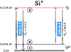 |
Fig. 1. Energy levels of the Si+ ion and transitions of Si II λ1526. P31 and P32 are the probabilities that a Si+ ion in level 3 radiatively de-excites to level 1 or 2. |
The dust opacity in every gas cell was computed assuming the implementation of Laursen et al. (2009) using the SMC law, as in Mauerhofer et al. (2021), Katz et al. (2023). In this model, the optical depth of dust is the product of a pseudo-density and a cross section. The pseudo-density is
 (1)
(1)
For the cross-section, we used the results of Gnedin et al. (2008) in the SMC case. This accounts for absorption and scattering events. For the albedo of dust grains, we used the values of Li & Draine (2001), which are 0.338 for Si II λ1260 and 0.431 for Si II λ1526. The direction in which a photon goes after scattering on dust was modelled with the Henyey-Greenstein function (Henyey & Greenstein 1941). This contains an asymmetry parameter g, also taken from Li & Draine (2001). It is 0.591 for Si II λ1260 and 0.575 for Si II λ1526.
After this setup, we computed the optical depth in each cell, and we took Si II λ1526 as an example:
 (2)
(2)
The optical depth of a given line in a gas cell is computed as  , where
  is the column density of ionised silicon in the ground state (fine-structure level) along the path in the cell, and the cross section is
 (3)
(3)
where fline is the oscillator strength of the line, λline is the central wavelength, and b is the Doppler parameter, which we explain below. Additionally, the variable a is defined by a = Alineλline/(4πb), where Aline is the Einstein coefficient of the line3. The variable x is a normalised wavelength shift from the line centre and is defined by x = (c/b)(λline − λcell)/λcell, where λcell is the wavelength of the photon packet in the frame of reference of the cell. We computed the Voigt function with the approximation of Smith et al. (2015).
When an interaction occured, one of the three channels of Equation (2) was randomly chosen with a probability τchannel/τcell. When the photon packet is absorbed by either the ground state or fine-structure level of Si+, it is re-emitted in a direction randomly drawn from an isotropic distribution. When the absorption channel is 1526.7 Å, the photon packet is re-emitted either via the same channel, as resonant scattering, or via the 1533.4 Å channel, which is fluorescent. The probabilities of the two channels are determined by the ratio of their Einstein coefficients, and they are shown in Fig. 1. Similarly, when the photon packet is absorbed by channel 1533.4 Å, it can be re-emitted at 1526.7 Å or at 1533.4 Å.
We explain the Doppler parameter b, which was updated compared to M21. It is a combination of thermal velocity and turbulent velocity vturb,
 (4)
(4)
where kb is the Boltzmann constant, T is the temperature, and mion is the mass of the interacting ion. In M21, we used a global constant vturb of 20 km s−1. To avoid using this free parameter, we now computed a turbulent velocity in each cell based on the nine density-weighted velocity gradients of the cell (three axis directions for vx, vy, and vz), which were computed from the properties of its direct neighbours. The resulting distribution of turbulent velocities has a volume-averaged value of ∼100 km s−1 and a density-averaged value of ∼25 km s−1, calculated within the virial radius of our simulated galaxies. Overall, this model of turbulence provides significantly broader absorption lines and fluorescent emission than the fiducial model of M21.
2.3. Computing line properties from spectra
The output absorption line spectra have a resolution of 10 km s−1 between −1500 km s−1 and vfluo + 1500 km s−1, where vfluo is the velocity of the fluorescent emission for each line. We used an aperture diameter of 2″, which means that the physical size of the aperture depended on redshift (∼ 8.5 − 13 kpc), but was always large enough to encompass the whole galaxy. To normalise the spectra, we divide them by the value of the continuum luminosity at their (flat) edges. We then computed the equivalent width (EWabs) of the absorption lines by integrating the spectra where the normalised luminosity is below 1 in a region from −1000 km s−1 to +600 km s−1 around the wavelength of the absorption. We defined EWabs to be positive. Then, the residual flux  of the lines was computed by taking the minimum flux of the normalised spectrum. Finally, the centroid velocity
  was computed by determining the velocity at which the absorption lines had half their EW. These measurements were made with the same method as in Gazagnes et al. (2023).
To illustrate the range of spectral properties in our sample, we selected representative spectra from each snapshot using KMeans clustering on key line properties, including the absorption equivalent width, residual flux, velocity centroid, and fluorescence strength. This procedure ensured that the selected spectra captured the diversity present in the simulations. These examples are shown in Fig. 2. The resulting spectra exhibit a variety of features: some lines are nearly symmetric (top left panel), while others are skewed (second row in the fourth column, or third row in the second column); the panel in the third row and first column shows an example of a profile with a secondary absorption feature; some LOS have no absorption; and the level of noise varies due to differing dust attenuation along the LOS.
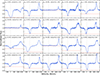 |
Fig. 2. Examples of Si II λ1526 absorption and fluorescent emission profiles drawn from different haloes and LOS among our seven simulation snapshots. The spectra were selected using KMeans clustering to span a diverse range of spectral properties, including the equivalent width of absorption, residual flux, velocity centroid, and fluorescence strength. Each panel shows the normalised spectrum (blue) along with a dashed horizontal line at the minimum flux level, and a vertical dotted grey line at line centre. The red line highlights the value of the residual flux, which is indicated at the top of each panel, along with the corresponding fesc. |
2.4. Computing the escape fraction of ionising photons
We are interested in predicting the LyC escape fraction using LIS absorption lines. While the data release of Katz et al. (2023) does contain values for fesc in ten viewing angles, it was computed only at a wavelength of 900 Å. We computed the escape fractions as in M21. To summarise, we sampled the intrinsic continuum of our galaxies from 200 Å up to the Lyman limit and propagated it until the virial radius using RASCAS. Photons interact with H0, He0, He+, and dust. The cross section of the interaction between ionising photons and H0 and He+ is computed analytically (Osterbrock & Ferland 2006),
 (5)
(5)
where ν is the frequency of the photon in Hz, assumed to be high enough to be ionising, Z is the nuclear charge (1 for H0 and 2 for He+), ν0 is the ionisation threshold frequency (13.6 eV or 54.4 eV over the Planck constant, for H0 and He+, respectively), and  . For the cross section of the interaction with He0, we used the approximation of Verner et al. (1996). For the dust cross section, we used the same implementation as for the non-ionising part, which included an extrapolation for ionising wavelengths (Gnedin et al. 2008; Laursen et al. 2009).
Just as for the RASCAS runs for the absorption lines, we used the peeling-off algorithm to measure the ionising continuum spectra in ten observation directions. The escape fraction is then simply the ratio of the integral of the escaping ionising continuum over the integral of the intrinsic ionising continuum. This provided us with the escape fraction of all ionising photons (fesc) and with the escape fraction of photons around 900 Å, which we computed from 890 Å to 910 Å ( ). The former is important when considering the contribution of galaxies to reionisation, while the latter is useful for a comparison with observations, since most of the time, we only have access to the ionising spectrum near 900 Å. The two escape fractions are included in the new data release. We show in Fig. 3 that both escape fractions have relatively similar values, with differences up to about 0.25 at maximum. In most cases,
  , since H I absorbs more photons at 900 Å than at lower wavelength (see Equation (5)). The rarer cases when
  can be explained by LOS where hydrogen is ionised, letting 900 Å photons pass, but the presence of helium absorbs a fraction of lower-wavelength photons.
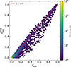 |
Fig. 3. Comparison of the escape fraction integrated over all ionising wavelengths on the x-axis and the escape fraction between 890 Å and 910 Å on the y-axis for all our simulated galaxies in the seven snapshots and in ten viewing angles. |
Finally, we summarise our model in Table 1 and compare it to the older model by M21. We highlight all the novelties of the present work. All the data files are described in Appendix B, and they are publicly available (see the section with the data availability).
3. Inferring fesc from Si II absorption lines
To show one possible use of this new data release, we explore how well we can infer fesc using the properties of our LIS absorption lines, such as the equivalent width of absorption, the residual flux, or the centroid velocity. Then, we explore whether using the dust attenuation factor as in M21 provides an accurate estimate of fesc when using a large number of galaxies with diverse properties rather than a single zoomed-in simulation.
3.1. Correlations with escape fractions
We now analyse whether some line properties correlate with the escape fraction of ionising photons. In Fig. 4 we show the relations between the escape fraction and three Si II λ1526 properties, that is, the residual flux, the equivalent width of the absorption, and the centroid velocity. In the following, we focus on this specific LIS line because we found that it yields better predictions than Si II λ1260. Some results using the latter line are shown in Appendix A, however.
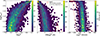 |
Fig. 4. Relations between the escape fraction of ionising photons and three Si II λ1526 properties. The solid lines show the running median, and the dashed lines show the 16th and 84th percentiles. These lines are affected by spectra with log(fesc) < − 3, which are not displayed here. The left and middle panels show the residual flux and equivalent width of the absorption line, respectively. The dotted pink line shows the upper limit found in M21. The right panel shows the centroid velocity of Si II λ1526. |
There is a weak correlation between fesc and the residual flux of Si II λ1526, as shown in the left panel of Fig. 4. Saturated lines, meaning lines with a residual flux below ∼0.1, almost all have an escape fraction below 10%. Most of the spectra with a residual flux above ∼0.75, that is, with weak absorption features, display a large escape fraction, fesc ≳ 5%. Except for these edge cases,  does not predict fesc.
The middle panel displays a poor correlation between the escape fraction and the EW of absorption. The only constraint we can derive is that spectra with a large EW rarely have an escape fraction above a few percent (e.g. only 0.9% of the spectra with EW > 1.5 Å have fesc > 5%). We also plot the upper limit that was found in M21 as a pink dotted line, and find that the SPHINX20 galaxies do not follow this limit. This is mainly because in our larger sample, some galaxies have escape fractions above the maximum of the isolated galaxy studied in that paper, and some galaxies have larger equivalent widths of the absorption.
Finally, the right panel shows no correlation between the escape fraction and the centroid velocity, which agrees with the results from Chisholm et al. (2017). The values below ∼ − 150 km s−1 are uncertain, since they are associated with spectra having little absorption, for which it is hard to measure the velocity of the line due to noise.
3.2. Dust correction to improve fesc predictions
Following M21 and the picket-fence model (e.g. Gazagnes et al. 2018; Saldana-Lopez et al. 2022), we applied a dust correction factor to the residual flux of absorption lines to predict a more accurate value for fesc. A better measure of the fraction of light that is absorbed by intervening dust and gas is not  , but the ratio of the flux at the bottom of the line over the flux of the intrinsic continuum. When we assume, as in the picket-fence model, that galaxies are partially covered by dense optically thick (in dust, H0 and Si+) gas, while the rest consists of empty holes, then the escape fraction of ionising photons fesc is indeed exactly equal to the ratio of the flux at the bottom of LIS absorption lines over the intrinsic continuum flux. Even though galaxies are not true picket fences, we show in Fig. 5 that we still obtain a much better approximation of fesc with this method. In this figure, the x-axis represents the residual flux of Si II λ1526 multiplied by the dust attenuation at 1500 Å. A direct comparison of spectra generated without dust would provide a complementary more idealised test, but this is beyond the scope of this work, which is focused on observations.
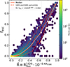 |
Fig. 5. Comparison of the escape fraction of ionising photons with the product of Si II λ1526 residual flux and the dust attenuation. The colour scale shows the number of spectra in each hexagonal bin. The solid orange line shows the running median, and the dashed lines show the 16th and 84th percentiles. The pink line shows the best power function fit to the data. While most of the points lie on the bottom left corner, around 5% of them have |

For comparison, we show the same results in Appendix A, but using Si II λ1260 instead of Si II λ1526. As we stated above, the former line yields poorer results with our method, with an increase of 42% in the prediction error of fesc.
We performed a fit of the data with a power function, which is shown by the pink line, and accurately fits the median relation (solid orange line). It has the form
 (6)
(6)
where  is the dust-correct residual flux, computed as
  , and A1500 is the dust attenuation at 1500 Å in units of magnitudes. This yields an average error on fesc of 0.0154 (0.0027 for
  and 0.0459 for
  ). To further quantify the accuracy of this method, we defined a leaking sightline as having an escape fraction of ionising photons higher than 10%. The completeness of this method for detecting leakers, that is, the fraction of leakers that we correctly identify compared to the total number of leakers, is 81.6%. The precision, which is the ratio of true positives over the sum of true positives and false positives, is 81.1%.
Finally, we applied the same procedure to predict  instead of fesc. We showed in Fig. 3 that the two quantities are close to each other, so we do not show a new figure here. The relation we found for the prediction of
  from the residual flux of Si II λ1526 and the dust attenuation factor is
 (7)
(7)
For clarity, all the errors discussed here are summarised in Table 2, which also includes the results obtained below for observationally derived dust attenuations (Section 4.2 and Appendix C). The table shows that the completeness and precision for  are similar to that for fesc, and the mean error on
  is only slightly smaller than the mean error on fesc. In the table, we also add mean absolute errors for probable leakers (
 ) and likely non-leakers (
 ). The error is naturally larger for probable leakers because the fesc values are higher. We chose to give the errors not in relative terms because then, predicting an escape fraction of 10−2 when the true value is 10−3 would yield a relative error of 900%, which is a large error, even though the prediction correctly assessed that the galaxy leaks only a small fraction of (≤1%) of ionising photons.
Comparison of fesc prediction accuracy and leaker classification performance using different A1500 estimates.
4. Discussion
Based on our numerous highly resolved simulated galaxies, we have demonstrated that the knowledge of the residual flux of LIS absorption lines, in particular, of Si II λ1526, may allow us to infer accurate escape fractions of ionising photons provided that we can perfectly correct for dust attenuation. When we applied this method to actual observations, a few limitations appeared that we discuss in Sections 4.1 and 4.2. In Section 4.3 we then apply our predictions to observed data for which the escape fraction was determined independently in order to test our method.
4.1. Measurement of the residual flux
The residual flux of absorption lines is challenging to measure observationally because the line-spread function and low resolution can smooth absorption profiles and thus artificially increase the residual flux. This has been extensively studied in Jennings et al. (2025), who applied observational effects to simulated spectra from the zoom-in simulation presented in M21, produced with the same mock observation method as in this paper. They degraded the simulated spectra following three different surveys characteristics, (a) LzLCS G140L (Flury et al. 2022a), (b) CLASSY (Berg et al. 2022), and (c) VANDELS (Garilli et al. 2021), whose resolutions (in terms of the full width at half-maximum σFWHM) are 300 km s−1, 65 km s−1, and 461 km s−1, respectively.
Their Figures 2 and 3 show that the resolution of LzLCS G140L and VANDELS is insufficient for capturing the residual flux of Si II λ1260 correctly. While the equivalent width is correctly inferred on average, the residual flux is mostly overestimated by ∼0.3 − 0.4 (absolute error), and sometimes up to ∼0.8 or underestimated by ∼0.2. For CLASSY, in contrast, the high resolution allows for a relatively faithful measurement of the residual flux, with errors generally around 0.05. Figure 5 of Jennings et al. (2025) also shows that a stacking analysis introduces another error in the measurement of the residual flux.
These errors explain a significant part of the discrepancy that we show in Section 4.3, since we did not apply observational effects when measuring the residual flux from our mock data.
4.2. Observational determination of the dust extinction
An additional uncertainty in the derivation of fesc is created by the biases and errors introduced by observational methods for deriving the UV dust attenuation factor. To quantify this, we tested three different codes (Cigale, LePhare, and FiCus) on our mock observations.
4.2.1. CIGALE
In order to reproduce a typical way of deriving the dust attenuation in observations of star-forming galaxies, we used the SED-fitting tool Code Investigating GALaxy Emission (CIGALE4: Boquien et al. 2019) applied to the 20 NIRCAM filter values provided in Katz et al. (2023) for our simulated galaxies. We assumed a double-exponential shape of the star formation history (SFH), a Chabrier IMF, the BPASS stellar library, and the SMC extinction law. We fixed the galaxy redshifts to their true value, and we allowed for a large number of values for EB − V. We note that for our galaxies at redshifts 4.64 and 5, we removed the bluest filter, NIRCAM F090W, from the fits because Katz et al. (2023) assumes that all photons below the rest-frame Lyman-α wavelength are absorbed by the IGM. However, at these two lowest SPHINX20 redshifts, this approximation is too strong because a non-negligible fraction of photons below this wavelength can propagate through the IGM. Since the bluest filter overlaps with wavelengths below the rest-frame Lyman-α at these two redshifts, we did not take the corresponding flux values into account.
We show the resulting predictions of the attenuation A1500 compared to the true values in Fig. 6. For most spectra with A1500 < 1, the CIGALE predictions of the attenuation are relatively accurate, although a few of them show a difference of up to one magnitude compared to the true value. For spectra with higher attenuations, CIGALE predictions are biased towards lower values: they underestimate the true attenuation. To study the reasons for this, we selected 140 galaxies with A1500 ≈ 2 mag and computed the dust optical depth in front of all the stellar particles of these galaxies by tracing rays with RASCAS. The distribution of the dust optical depth shows that galaxies with a high optical depth in front of the brightest star clusters always have their dust attenuation underestimated by CIGALE by at least one magnitude. Galaxies with a more homogeneous cover of dust in front of all stars can be either correctly predicted or not. It is understandable that A1500 is underestimated by CIGALE for galaxies with optically thick dust in front of bright star clusters because these clusters do not contribute to the UV spectra at all (and often not even to the optical spectra), and thus, are missed by the SED fitting. A knowledge of the dust emission in the infrared would help us to better constrain the dust attenuation.
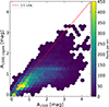 |
Fig. 6. Dust attenuation at 1500 Å predicted by CIGALE compared to the true attenuation (see details of the CIGALE implementation in Sect. 4.2.1). |
We recomputed the errors of our models (Eq. (6)), except with A1500 predicted by CIGALE instead of the true value from the simulation, and we list the answers in Table 2. We obtain an average error on fesc of 0.0238 (0.003 for  and 0.0513 for
  ). For the detection of leakers (with fesc > 0.1), the completeness increases from 81.6% to 87.3%, meaning that more true leakers are correctly identified. However, the precision decreases significantly, from 81.1% to 67.6%, which means that almost one-third of the galaxies identified as leakers actually have low escape fractions. This is expected because the dust attenuation is underestimated by CIGALE on average, and Equation (6) shows that fesc is overestimated. While less accurate than when using the real dust attenuation, these predictions of fesc are still mostly reliable and useful. We found similar results with another SED-fitting code, LEPHARE, which we show in Appendix C.
4.2.2. F ICUS
Finally, we also tested a different approach, using the spectral fitting tool FItting the stellar Continuum of Uv Spectra (FICUS5: Saldana-Lopez et al. 2023), applied to SPHINX20 continuum spectra from 1200 Å to 2000 Å, and assuming the SMC extinction law. These spectra were obtained with RASCAS, including only the interaction of photons with dust, not with metallic ions, since LIS absorption lines are masked by FICUS in any case. The fiducial version of FICUS uses a combination of STARBURST99 (Leitherer et al. 1999) and BPASS stellar templates, including a model of the nebular continuum, but since we did not model this nebular component, we used a modified version of FICUS with the stellar continuum from BPASS alone. The predictions of FICUS for the dust attenuation are shown in Fig. 7. The results we found are similar to those for the SED-fitting codes in that high A1500 values are underestimated by FICUS. Additionally, we found that it slightly overestimates A1500 in the low dust attenuation regime. Thus, the mean errors on fesc are slightly larger than for CIGALE and LEPHARE, at 0.0243 (0.0030 for  and 0.0634 for
  ; see more details in Table 2).
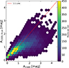 |
Fig. 7. Dust attenuation predicted by FICUS compared to the true attenuation. |
In summary, all three methods show that they cannot infer the intrinsic UV continuum accurately when A1500 ≳ 1 − 1.5. This is an expected result because strongly attenuated zones in a galaxy are strongly dominated in the integrated spectrum by low-attenuation zones (e.g. Gazagnes et al. 2023). Despite this, the errors they introduce when inferring the escape fraction with our new method are small. This is in part due to the fact that galaxies with strong dust attenuation, for which the inferred A1500 are the most inaccurate, usually have almost no escape of ionising photons (fesc ≈ 0).
4.3. Applying our method to observations
Equipped with a simple relation between absorption line depth, dust attenuation, and escape fraction, we applied our predictions to observed data of galaxies with independent estimates of fesc to test whether the limitations listed above still result in a good agreement. Since only the LyC close to the Lyman limit can be observed, we used our Equation (7) to predict  .
.
4.3.1. LzLCS
The LzLCS sample (Flury et al. 2022a,b) contains 66 star-forming galaxies observed with the Cosmic Origins Spectrograph (COS) on the Hubble Space Telescope (HST), including coverage on the LyC. It is an ideal dataset to test our predictions of the escape fraction of ionising photons. Using a public database of LzLCS galaxy properties in addition to 23 leakers compiled from previous studies (Izotov et al. 2016a,b, 2018, 2021; Wang et al. 2019), we read the UV dust attenuation estimated for each galaxy (assuming the SMC extinction law) as well as the residual flux of absorption lines. Unfortunately, the Si II λ1526 line is not observed in this sample because it falls outside the wavelength range of HST/COS, so we instead relied on an average residual flux of all LIS lines they detected (Si II λλ1190, 1193, Si II λ1260, O I λ1302, and C II λ1334), called RLIS. Assuming the error on dust attenuation and residual flux provided by the LzLCS data follows a Gaussian distribution, we estimated the error on the escape fraction via a Monte Carlo sampling of Equation (7). This prediction of  can then be compared to the escape fraction inferred from the LyC of the LzLCS sample. Flury et al. (2022a) presented three different ways of inferring the escape fractions. We adopted the UV SED fesc, which they determined to be the most reliable. It is the ratio of the measured LyC flux to the intrinsic LyC flux given by the best-fit STARBURST99 templates computed with FICUS, and we call it
  . We present the comparison of our prediction of LzLCS escape fractions (
 ) versus the measurements of Flury et al. (2022a) in Fig. 8. The match is good overall, although the error bars are large, and for some galaxies, the prediction does not match the measured
  even within the errors. For example, the eight galaxies with
  are predicted to have values that are lower by two to four times with our method. Additionally, the vast majority of galaxies with upper limits on
  in LzLCS (empty symbols in Fig. 8) are predicted to have non-negligible escape fractions, above a few percent.
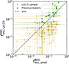 |
Fig. 8. Comparison of Equation (7) applied to LzLCS residual fluxes and dust attenuations (x-axis) with |

These discrepancies can be understood from several factors. We showed in Sect. 4.1 that the LzLCS survey characteristics tend to degrade absorption lines, leading to inaccurate determinations of the residual flux. In particular, the absorption is spread, artificially increasing the residual flux. This effect would cause our predictions to be higher than the actual values. Additionally, we showed in Sect. 4.2.2 that the measurements of dust attenuation with observed UV spectra are relatively inaccurate. The dust attenuation determinations for LzLCS galaxies are indeed performed with FICUS. Fig. 7 shows that FICUS slightly overestimates A1500 on average for galaxies with no or very low dust attenuation. From Equation (7), this causes our prediction of  to underestimate the true escape fraction. This partly explains the mismatch for the eight leakiest galaxies in Fig. 8, which indeed have a very low dust attenuation. In contrast, for galaxies with strong dust attenuation, Fig. 7 shows that FICUS underestimates A1500, which causes Equation (7) to overestimate
  . This can explain why many LzLCS upper limits are predicted to have non-negligible escape fractions by our method. An additional reason for the underestimation of fesc for the eight leakiest galaxies might be that in our simulations, we did not allow for the escape of nebular LyC photons, which Izotov et al. (2025) found to be a non-negligible component for several leakers observed with COS. Another source of discrepancy, as mentioned above, comes from the fact that we were unable to use Si II λ1526 for our analysis because it is not in the LzLCS dataset. It is unclear how much this affects our predictions, but the residual fluxes of different LIS lines of oxygen, silicon, and carbon have been shown to be relatively similar (e.g. Steidel et al. 2018; Parker et al. 2024). Therefore, we expect that this caveat in our work does not introduce a significant systematic bias, but only contributes slightly to the scatter in the data. Finally, another source of discrepancy between the two quantities in Fig. 8 is the fact that our equation for the prediction of
  is based on the true escape fractions from simulated galaxies, while this quantity is not directly measurable. For a more direct comparison, the methods of Flury et al. (2022a) should be applied to infer
  directly to mock data of our simulated galaxies. This is beyond our scope, in part because not all the relevant mock data have been created yet.
4.3.2. CLASSY
Another sample of galaxies to test our method comes from the CLASSY survey (Berg et al. 2022; James et al. 2022), which consists of 45 low-redshift (z < 0.18) star-forming galaxies with diverse characteristics in terms of mass, star formation rate, dust attenuation, and so on. With a maximum resolution of R ∼ 15 000 (Berg et al. 2022), the residual flux of absorption lines can be measured with higher precision than for LzLCS galaxies (R ∼ 1000), and the wavelength range covered by CLASSY allowed us to use the Si II λ1526 line for almost all its galaxies. However, the redshifts of CLASSY galaxies are too low for HST/COS to be able to detect ionising photons. Instead, we followed Parker et al. (2026), who applied numerous indirect methods for determining  and applied them to the high-quality CLASSY spectra. We summarise the escape fractions from that study below.
-
 uses LIS absorption lines to infer the covering fraction of LIS metals and in turn of H0 to derive a value of
  . This is based on Chisholm et al. (2018), Saldana-Lopez et al. (2022), Parker et al. (2024).
 -
 uses the trend between the β slope of the UV continuum and
  , as found by Chisholm et al. (2022).
 -
 uses the peak separation of the Lyman-α line, when detected, which was shown to trace
  by numerous studies (e.g. Verhamme et al. 2017; Izotov et al. 2018; Flury et al. 2022b), although the trend was found to not work at higher redshifts (e.g. Kerutt et al. 2024).
 -
 uses multivariate statistical analysis performed in Jaskot et al. (2024a,b), based on many properties such as stellar mass, E(B−V)∗, E(B−V)neb, SFR, the star formation rate surface density, M1500, βUV, the ionisation ratio O32, and the equivalent width of the Hβ emission line.
 -
 uses results from Gazagnes et al. (2023), who fitted mock C II λ1334 and Si II λ1260 absorption lines to CLASSY galaxies. These mock spectra were obtained from the cosmological zoom-in simulation presented in M21, using the same method as presented in Sect. 2.2. Processing the simulated galaxy at different times and from many viewing angles, this provides a catalogue of 22 500 mock spectra for both lines. For 38 of the 45 CLASSY galaxies, an excellent match is found in this catalogue by fitting both lines simultaneously. For these galaxies,
  is defined as the escape fraction of the simulated galaxy at the time and viewing angle of the best-match spectrum.
 -
 uses the emission line ratio O32 = [O III] λ5007/[O II] λ3727, which was shown to correlate with
  in some studies (e.g. Izotov et al. 2016a, 2018; Nakajima et al. 2020).
 -
 is the median escape fraction from Parker et al. (2026), obtained by taking the median of the six previous
  estimates. The uncertainties for this median are defined as the 16th and 84th percentiles from 300 Monte Carlo variations of the individual escape fraction predictions based on their uncertainties.
Not all these six indirect tracers of  are fully independent becaue both
  and
and  use the ratio O32, βUV is used in
  and
and  , and LIS absorption lines are used in
  and
and  . The correlations between the different methods, as well as their biases as a function of dust attenuation or neutral gas covering fraction, are analysed in detail in Parker et al. (2026).
Our predictions of  for CLASSY galaxies are labelled
  , and, along with error bars, were computed as in Sect. 4.3.1, except that we used the Si II λ1526 line. A few CLASSY galaxies do not include this line, and we therefore omitted them. Comparisons with the escape fractions of Parker et al. (2026) are shown in Fig. 9, in order of increasing
  . Because our predictions are ill-suited for distinguishing escape fractions below one percent, we used a linear scale for the y-axis. For clarity, our main comparison was made with the median
  (purple points), while the points from the six methods presented above are shown in grey for completeness. The figure shows that our predictions are close to the median,
  . For most galaxies below the weak leaker threshold of 5%, our predictions match the median
  within the error bars. A slight discrepancy arises only for J1521+0759. For one weak leaker, J1016+3754, our method predicts larger escape fractions, around 15%, compared to 5% for the median of Parker et al. (2026). Our prediction is compatible with
  , which might indicate that LIS absorption lines in this faint (M1500 ∼ −14) galaxy overpredict the true escape fraction. This might be due to its low metallicity (12 + log(O/H) ∼ 7.5), which can result in weak LIS absorption lines, while H0 still absorbs many ionising photons. Our method also overestimates the escape fraction of J0934+5514, which is an even fainter and more metal-poor galaxy. Overall, the global compatibility of our predictions with the many methods presented in Parker et al. (2026) is encouraging for the use of LIS residual flux and dust attenuation to predict the escape fraction of ionising photons at the epoch of reionisation.
 |
Fig. 9. Comparison of our predictions of |


5. Summary and conclusions
We have extended the SPHINX20 data release with high-resolution synthetic LIS absorption lines, modelled with full radiative transfer and including detailed physics such as resonant scattering, dust interactions, turbulence, and absorption from the fine-structure level. Using this dataset, we analysed correlations between Si II λ1526 absorption properties, dust attenuation, and the escape fraction of ionising photons ( ). We also tested how well our results apply to observational data and assessed common observational techniques for inferring dust attenuation. Our main conclusions are listed below.
-
We found a tight correlation between the dust-corrected residual flux of the Si II λ1526 line and the escape fraction of ionising photons, which we expressed as a simple empirical power law (Eq. (6)). This relation predicts
 with an average error below 0.02.
 -
The predictive power of this method is strongest when using high-resolution spectra and accurate estimates of the UV dust attenuation. When using true attenuation values from the simulation, our method achieves 82% precision and completeness in identifying leakers (
 ).
). -
We showed that several commonly used methods to infer A1500, namely CIGALE, LEPHARE, and FICUS, often underestimate the true attenuation, especially in dusty galaxies where bright star-forming regions are heavily obscured. This leads to systematic overestimates of
 when applying our formula. However, since most leakers have relatively low dust attenuation, using observationally inferred values of the dust attenuation usually does not introduce strong errors for them.
 -
Application of our method to the LzLCS survey yielded mixed results, with significant scatter and poor agreement for several galaxies, while the escape fraction of others was correctly predicted. We attribute the discrepancies to the limited spectral resolution of the HST/COS G140L grating, the lack of the Si II λ1526 line, and uncertain dust estimates from the SED-fitting codes.
-
In contrast, when we applied the same method to CLASSY galaxies, where both Si II λ1526 and high-resolution UV spectra are available, the results agree well on average with the median
 values inferred from six independent (indirect) observational techniques.
 -
The new dataset of LIS absorption lines, combined with ionising escape fractions and galaxy properties, provides a valuable public resource for testing ISM diagnostics and spectrum-fitting techniques. The data are made publicly available (see the section Data availability).
-
Overall, our work supports the use of LIS absorption lines, in particular Si II λ1526, as observational tracers of
 at the epoch of reionisation, but it highlights that their effectiveness critically depends on our ability to reliably measure the line depth and dust attenuation.
Despite the robustness of our results, several caveats remain. First, while our predictive formula performs well within the simulation, it is calibrated on a specific model of galaxy formation, feedback, and dust attenuation (Rosdahl et al. 2022). Applying it to observations assumes that similar physical conditions hold. Second, our modelling of the silicon ion density assumes solar abundance ratios scaled to local metallicity, along with equilibrium ionisation fractions computed using a fixed radiation field. Both assumptions may introduce uncertainties, particularly in high-redshift and low-density environments. Lastly, the simulation adopts an SMC-like extinction curve and a fixed dust-to-metal scaling, which may not capture the full diversity of dust physics in real galaxies. Processes such as gas–dust decoupling, dust destruction by sputtering, and shocks may lead to different dust opacities and different star-dust geometries compared to our current work. This might alter the quantitative relation between LIS residual flux and fesc, for example by introducing additional scatter or modifying the normalisation of the inferred trends. However, the magnitude and direction of these effects are currently uncertain, and further developments in dust modelling are necessary before these effects can be analysed.
The approach we presented can be expanded in several directions. A logical next step is to apply this method to larger samples of high-resolution UV spectra, especially with upcoming surveys targeting star-forming galaxies at higher redshifts. Our data might also serve as training sets for machine-learning models designed to infer  directly from spectra. Additionally, extending this analysis to include emission line diagnostics and their connection to the escape of ionising radiation (e.g. Choustikov et al. 2024) would help us to unify the absorption and emission line approaches to reionisation-era galaxy studies. Finally, new-generation simulations such as MEGATRON (Katz et al. 2026) remove many of the limitations cited above and might create robuster predictions of the escape fraction of ionising photons.
Data availability
The spectra, absorption line measurements, and escape fraction values used in this work are publicly available at https://doi.org/10.5281/zenodo.17723577
Acknowledgments
VM acknowledges support from the NWO grant 016.VIDI.189.162 (‘ODIN’). T.K. is supported by the National Research Foundation of Korea (RS-2022-NR070872 and RS-2025-00516961) and also by the Yonsei Fellowship, funded by Lee Youn Jae.
References
- Arnouts, S., & Ilbert, O. 2011, Astrophysics Source Code Library [record ascl:1108.009] [Google Scholar]
- Asplund, M., Amarsi, A. M., & Grevesse, N. 2021, A&A, 653, A141 [NASA ADS] [CrossRef] [EDP Sciences] [Google Scholar]
- Badnell, N. R. 2006, ApJS, 167, 334 [Google Scholar]
- Berg, D. A., James, B. L., King, T., et al. 2022, ApJS, 261, 31 [NASA ADS] [CrossRef] [Google Scholar]
- Bergvall, N., Zackrisson, E., Andersson, B. G., et al. 2006, A&A, 448, 513 [NASA ADS] [CrossRef] [EDP Sciences] [Google Scholar]
- Boquien, M., Burgarella, D., Roehlly, Y., et al. 2019, A&A, 622, A103 [NASA ADS] [CrossRef] [EDP Sciences] [Google Scholar]
- Borthakur, S., Heckman, T. M., Leitherer, C., & Overzier, R. A. 2014, Science, 346, 216 [Google Scholar]
- Carr, C., Scarlata, C., Panagia, N., & Henry, A. 2018, ApJ, 860, 143 [Google Scholar]
- Chisholm, J., Orlitová, I., Schaerer, D., et al. 2017, A&A, 605, A67 [NASA ADS] [CrossRef] [EDP Sciences] [Google Scholar]
- Chisholm, J., Gazagnes, S., Schaerer, D., et al. 2018, A&A, 616, A30 [NASA ADS] [CrossRef] [EDP Sciences] [Google Scholar]
- Chisholm, J., Saldana-Lopez, A., Flury, S., et al. 2022, MNRAS, 517, 5104 [CrossRef] [Google Scholar]
- Choustikov, N., Katz, H., Saxena, A., et al. 2024, MNRAS, 529, 3751 [NASA ADS] [CrossRef] [Google Scholar]
- De Cia, A., Ledoux, C., Mattsson, L., et al. 2016, A&A, 596, A97 [NASA ADS] [CrossRef] [EDP Sciences] [Google Scholar]
- Eldridge, J. J., Izzard, R. G., & Tout, C. A. 2008, MNRAS, 384, 1109 [Google Scholar]
- Erb, D. K. 2015, Nature, 523, 169 [Google Scholar]
- Fan, X., Carilli, C. L., & Keating, B. 2006, ARA&A, 44, 415 [Google Scholar]
- Flury, S. R., Jaskot, A. E., Ferguson, H. C., et al. 2022a, ApJS, 260, 1 [NASA ADS] [CrossRef] [Google Scholar]
- Flury, S. R., Jaskot, A. E., Ferguson, H. C., et al. 2022b, ApJ, 930, 126 [NASA ADS] [CrossRef] [Google Scholar]
- Garel, T., Michel-Dansac, L., Verhamme, A., et al. 2024, A&A, 691, A213 [NASA ADS] [CrossRef] [EDP Sciences] [Google Scholar]
- Garilli, B., McLure, R., Pentericci, L., et al. 2021, A&A, 647, A150 [NASA ADS] [CrossRef] [EDP Sciences] [Google Scholar]
- Gazagnes, S., Chisholm, J., Schaerer, D., et al. 2018, A&A, 616, A29 [NASA ADS] [CrossRef] [EDP Sciences] [Google Scholar]
- Gazagnes, S., Mauerhofer, V., Berg, D. A., et al. 2023, ApJ, 952, 164 [NASA ADS] [CrossRef] [Google Scholar]
- Gazagnes, S., Cullen, F., Mauerhofer, V., et al. 2024, ApJ, 969, 50 [NASA ADS] [CrossRef] [Google Scholar]
- Gnedin, N. Y., Kravtsov, A. V., & Chen, H.-W. 2008, ApJ, 672, 765 [Google Scholar]
- Grassi, T., Bovino, S., Schleicher, D. R. G., et al. 2014, MNRAS, 439, 2386 [Google Scholar]
- Haardt, F., & Madau, P. 2012, ApJ, 746, 125 [Google Scholar]
- Heckman, T. M., Borthakur, S., Overzier, R., et al. 2011, ApJ, 730, 5 [Google Scholar]
- Heckman, T. M., Alexandroff, R. M., Borthakur, S., Overzier, R., & Leitherer, C. 2015, ApJ, 809, 147 [Google Scholar]
- Henyey, L. G., & Greenstein, J. L. 1941, ApJ, 93, 70 [Google Scholar]
- Izotov, Y. I., Orlitová, I., Schaerer, D., et al. 2016a, Nature, 529, 178 [Google Scholar]
- Izotov, Y. I., Schaerer, D., Thuan, T. X., et al. 2016b, MNRAS, 461, 3683 [Google Scholar]
- Izotov, Y. I., Worseck, G., Schaerer, D., et al. 2018, MNRAS, 478, 4851 [Google Scholar]
- Izotov, Y. I., Worseck, G., Schaerer, D., et al. 2021, MNRAS, 503, 1734 [NASA ADS] [CrossRef] [Google Scholar]
- Izotov, Y. I., Schaerer, D., Worseck, G., et al. 2025, A&A, 704, A19 [NASA ADS] [CrossRef] [EDP Sciences] [Google Scholar]
- James, B., & Aloisi, A. 2018, ApJ, 853, 124 [Google Scholar]
- James, B. L., Aloisi, A., Heckman, T., Sohn, S. T., & Wolfe, M. A. 2014, ApJ, 795, 109 [NASA ADS] [CrossRef] [Google Scholar]
- James, B. L., Berg, D. A., King, T., et al. 2022, ApJS, 262, 37 [NASA ADS] [CrossRef] [Google Scholar]
- Jaskot, A. E., Silveyra, A. C., Plantinga, A., et al. 2024a, ApJ, 972, 92 [NASA ADS] [CrossRef] [Google Scholar]
- Jaskot, A. E., Silveyra, A. C., Plantinga, A., et al. 2024b, ApJ, 973, 111 [NASA ADS] [CrossRef] [Google Scholar]
- Jennings, R. M., Henry, A., Mauerhofer, V., et al. 2025, ApJ, 979, 64 [Google Scholar]
- Katz, H., Rosdahl, J., Kimm, T., et al. 2022, MNRAS, 510, 5603 [NASA ADS] [CrossRef] [Google Scholar]
- Katz, H., Rosdahl, J., Kimm, T., et al. 2023, Open J. Astrophys., 6, 44 [NASA ADS] [CrossRef] [Google Scholar]
- Katz, H., Rey, M. P., Cadiou, C., Kimm, T., & Agertz, O. 2026, Open J. Astrophys., 9, 56097 [Google Scholar]
- Kerutt, J., Oesch, P. A., Wisotzki, L., et al. 2024, A&A, 684, A42 [NASA ADS] [CrossRef] [EDP Sciences] [Google Scholar]
- Kimm, T., Cen, R., Devriendt, J., Dubois, Y., & Slyz, A. 2015, MNRAS, 451, 2900 [CrossRef] [Google Scholar]
- Konstantopoulou, C., De Cia, A., Krogager, J.-K., et al. 2022, A&A, 666, A12 [NASA ADS] [CrossRef] [EDP Sciences] [Google Scholar]
- Laursen, P., Sommer-Larsen, J., & Andersen, A. C. 2009, ApJ, 704, 1640 [Google Scholar]
- Leitet, E., Bergvall, N., Hayes, M., Linné, S., & Zackrisson, E. 2013, A&A, 553, A106 [NASA ADS] [CrossRef] [EDP Sciences] [Google Scholar]
- Leitherer, C., Schaerer, D., Goldader, J. D., et al. 1999, ApJS, 123, 3 [Google Scholar]
- Leitherer, C., Hernandez, S., Lee, J. C., & Oey, M. S. 2016, ApJ, 823, 64 [Google Scholar]
- Li, A., & Draine, B. T. 2001, ApJ, 554, 778 [Google Scholar]
- Luridiana, V., Morisset, C., & Shaw, R. A. 2015, A&A, 573, A42 [NASA ADS] [CrossRef] [EDP Sciences] [Google Scholar]
- Marques-Chaves, R., Schaerer, D., Amorín, R. O., et al. 2022, A&A, 663, L1 [NASA ADS] [CrossRef] [EDP Sciences] [Google Scholar]
- Mauerhofer, V., Verhamme, A., Blaizot, J., et al. 2021, A&A, 646, A80 [NASA ADS] [CrossRef] [EDP Sciences] [Google Scholar]
- Michel-Dansac, L., Blaizot, J., Garel, T., et al. 2020, A&A, 635, A154 [EDP Sciences] [Google Scholar]
- Nakajima, K., Ellis, R. S., Robertson, B. E., Tang, M., & Stark, D. P. 2020, ApJ, 889, 161 [NASA ADS] [CrossRef] [Google Scholar]
- Osterbrock, D. E., & Ferland, G. J. 2006, Astrophysics of Gaseous Nebulae and Active Galactic Nuclei (Sausalito, CA: University Science Books) [Google Scholar]
- Ouchi, M., Harikane, Y., Shibuya, T., et al. 2018, PASJ, 70, S13 [Google Scholar]
- Parker, K. S., Berg, D. A., Gazagnes, S., et al. 2024, ApJ, 977, 104 [NASA ADS] [CrossRef] [Google Scholar]
- Parker, K. S., Berg, D. A., Chisholm, J., et al. 2026, ApJ, 997, 98 [Google Scholar]
- Prochaska, J. X., Kasen, D., & Rubin, K. 2011, ApJ, 734, 24 [Google Scholar]
- Puschnig, J., Hayes, M., Östlin, G., et al. 2017, MNRAS, 469, 3252 [Google Scholar]
- Reddy, N. A., Steidel, C. C., Pettini, M., Bogosavljević, M., & Shapley, A. E. 2016, ApJ, 828, 108 [Google Scholar]
- Rivera-Thorsen, T. E., Hayes, M., & Melinder, J. 2022, A&A, 666, A145 [NASA ADS] [CrossRef] [EDP Sciences] [Google Scholar]
- Rosdahl, J., Blaizot, J., Aubert, D., Stranex, T., & Teyssier, R. 2013, MNRAS, 436, 2188 [Google Scholar]
- Rosdahl, J., Katz, H., Blaizot, J., et al. 2018, MNRAS, 479, 994 [NASA ADS] [Google Scholar]
- Rosdahl, J., Blaizot, J., Katz, H., et al. 2022, MNRAS, 515, 2386 [CrossRef] [Google Scholar]
- Saldana-Lopez, A., Schaerer, D., Chisholm, J., et al. 2022, A&A, 663, A59 [NASA ADS] [CrossRef] [EDP Sciences] [Google Scholar]
- Saldana-Lopez, A., Schaerer, D., Chisholm, J., et al. 2023, MNRAS, 522, 6295 [NASA ADS] [CrossRef] [Google Scholar]
- Saxena, A., Pentericci, L., Ellis, R. S., et al. 2022, MNRAS, 511, 120 [NASA ADS] [CrossRef] [Google Scholar]
- Scarlata, C., & Panagia, N. 2015, ApJ, 801, 43 [Google Scholar]
- Shapley, A. E., Steidel, C. C., Pettini, M., & Adelberger, K. L. 2003, ApJ, 588, 65 [Google Scholar]
- Smith, A., Safranek-Shrader, C., Bromm, V., & Milosavljević, M. 2015, MNRAS, 449, 4336 [Google Scholar]
- Stanway, E. R., Eldridge, J. J., & Becker, G. D. 2016, MNRAS, 456, 485 [NASA ADS] [CrossRef] [Google Scholar]
- Steidel, C. C., Erb, D. K., Shapley, A. E., et al. 2010, ApJ, 717, 289 [Google Scholar]
- Steidel, C. C., Bogosavljević, M., Shapley, A. E., et al. 2018, ApJ, 869, 123 [Google Scholar]
- Teyssier, R. 2002, A&A, 385, 337 [CrossRef] [EDP Sciences] [Google Scholar]
- Vanzella, E., Siana, B., Cristiani, S., & Nonino, M. 2010, MNRAS, 404, 1672 [NASA ADS] [Google Scholar]
- Vanzella, E., de Barros, S., Castellano, M., et al. 2015, A&A, 576, A116 [NASA ADS] [CrossRef] [EDP Sciences] [Google Scholar]
- Vanzella, E., Nonino, M., Cupani, G., et al. 2018, MNRAS, 476, L15 [Google Scholar]
- Verhamme, A., Orlitová, I., Schaerer, D., et al. 2017, A&A, 597, A13 [NASA ADS] [CrossRef] [EDP Sciences] [Google Scholar]
- Verner, D. A., Ferland, G. J., Korista, K. T., & Yakovlev, D. G. 1996, ApJ, 465, 487 [Google Scholar]
- Voronov, G. S. 1997, At. Data Nucl. Data Tables, 65, 1 [Google Scholar]
- Wang, B., Heckman, T. M., Leitherer, C., et al. 2019, ApJ, 885, 57 [NASA ADS] [CrossRef] [Google Scholar]
- Wise, J. H. 2019, Contemp. Phys., 60, 145 [NASA ADS] [CrossRef] [Google Scholar]
- Xu, X., Heckman, T., Henry, A., et al. 2023, ApJ, 948, 28 [NASA ADS] [CrossRef] [Google Scholar]
All the line parameters are taken from the NIST atomic database https://www.nist.gov/pml/atomic-spectra-database
Appendix A: Si II 1260 plots
For completeness, we show here the equivalent of Fig.1 and 5 but using Si II λ1260 instead of Si II λ1526. In Fig.A.1 we show that the atomic structure related to Si II λ1260 is slightly more complex than for Si II λ1526, with the upper level being split into two fine-structure levels. All of the transitions displayed are included in our RASCAS modelling.
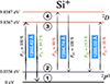 |
Fig. A.1. Energy levels of the Si+ ion and transitions of Si II λ1260. P13 = 100% indicates that a Si+ ion in level 1 can be photo-excited only to level 3. The green numbers are the probabilities that a Si+ ion in level 3 radiatively de-excites to level 1 or 2. The red numbers are the probabilities that an incoming photon with a wavelength between 1264.74 Å and 1265.0 Å hitting a Si+ ion in level 2 excites it to level 3 or 4. P42 = 100% indicates that a Si+ ion in level 4 can only radiatively de-excite to level 2. |
Then, in Fig.A.2, we show the relation between the dust-corrected residual flux of Si II λ1260 (called  ) and the escape fraction. Contrarily to Fig.5, we use here A1300 instead of A1500, since it is closer in wavelength to Si II λ1260. It is clear that using Si II λ1260 results in a wider dispersion. The mean error is 0.0218, which is 42% larger than when using Si II λ1526 (see Table 2). This explains why we use the latter line in the analysis of this paper.
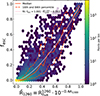 |
Fig. A.2. Comparison of the escape fraction of ionising photons with the product of Si II λ1260 residual flux and the dust attenuation (i.e. the dust-corrected residual flux). The colour scale shows the number of spectra in each hexagonal bin. The solid orange line shows the running median while the dashed lines show the 16th and 84th percentiles. The pink line shows the best power function fit to the data. |
Appendix B: Content of the LIS data release
The tables and the spectra in JSON format are freely available at the following URL: https://doi.org/10.5281/zenodo.17723577. A dedicated Jupyter notebook is also provided to illustrate how to read the files and plot example spectra.
All the data about line properties and dust attenuation is in the table line_properties.csv. This table lists, for each simulated halo (halo_id) and its corresponding redshift, the properties of the Si II absorption and fluorescent emission lines measured along ten different viewing directions (dir_0–dir_9). For the Si II λ1260 and Si II λ1526 absorption lines, the table includes the residual flux (res_flux), equivalent width (EW), velocity at minimum flux (v_max), and centroid velocity (v_cen). The Si II λ1265 and Si II λ1533 entries correspond to their respective fluorescent emission counterparts, with only the equivalent widths recorded. For each LOS, the table also provides the UV attenuation at 1500Å (A1500), both the value directly measured from the simulation and the values inferred through SED-fitting or spectral-fitting approaches with CIGALE, LEPHARE, and FICUS. More halo properties are in the original data release (Katz et al. 2023), in the all_basic_data.csv table.
Then, data about the escape fractions computed in this work is in the table fesc_table.csv. This table provides, for each simulated halo (halo_id) and its corresponding redshift, the escape fraction of ionising photons (fesc) measured along ten different viewing directions (dir_0–dir_9). For each direction, two quantities are reported: the total escape fraction integrated over all ionising wavelengths (fesc_dir_X) and the escape fraction measured specifically at 900 Å (fesc_900_dir_X). The column fesc_angle_avg gives the angle-averaged escape fraction, defined as the ratio between the total number of ionising photons escaping the galaxy in all directions and the total number intrinsically produced. The quantity intrinsic_nion corresponds to the intrinsic ionising photon production rate of the galaxy (in photons s−1). Similarly, intrinsic_nion_900 is the intrinsic production rate of photons at 900 Å, in photons s−1 Å−1.
Finally, the data release also includes the synthetic Si II spectra for all galaxies at all seven redshifts. Each file (e.g. SiII_1260_spectra_z6.json) contains the spectra along ten viewing directions for all galaxies at the corresponding redshift. The Si II λ1260 and Si II λ1526 files include both the absorption and associated fluorescent emission lines within the same spectrum.
Appendix C: Predicting A1500 with LEPHARE
For comparison with Section 4.2.1, where we used CIGALE, here we test another independent SED-fitting tool based on photometric measurements, LEPHARE (Arnouts & Ilbert 2011)6. We build SFH models using our stellar library BPASSV2.2.1 and assume a delayed exponentially declining star-formation history. For the dust attenuation, we choose the SMC extinction law to match our RASCAS models. Like for CIGALE, we removed the bluest filter for galaxies at redshifts 4.64 and 5 (see Sect. 4.2.1). The resulting predictions of the attenuation A1500 are shown in Fig.C.1. Globally, with our setups, LEPHARE predictions are similarly accurate as with CIGALE, as shown in Table 2. Attenuations above ∼1.5 mag are on average underestimated. The average error on fesc is 0.0215 (0.0028 for  and 0.0566 for
  ). The completeness is 80.7%, just slightly lower than with the real dust attenuation, and the precision is 78.3%, just lower than with the real A1500 and better than with CIGALE’s A1500. The interpretation of those finding is the same as in Sect. 4.2.1.
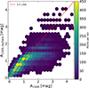 |
Fig. C.1. Dust attenuation at 1500 Å predicted by LEPHARE compared to the true attenuation. |
All Tables
Comparison of fesc prediction accuracy and leaker classification performance using different A1500 estimates.
All Figures
|
Fig. 1. Energy levels of the Si+ ion and transitions of Si II λ1526. P31 and P32 are the probabilities that a Si+ ion in level 3 radiatively de-excites to level 1 or 2. |
| In the text | |
|
Fig. 2. Examples of Si II λ1526 absorption and fluorescent emission profiles drawn from different haloes and LOS among our seven simulation snapshots. The spectra were selected using KMeans clustering to span a diverse range of spectral properties, including the equivalent width of absorption, residual flux, velocity centroid, and fluorescence strength. Each panel shows the normalised spectrum (blue) along with a dashed horizontal line at the minimum flux level, and a vertical dotted grey line at line centre. The red line highlights the value of the residual flux, which is indicated at the top of each panel, along with the corresponding fesc. |
| In the text | |
|
Fig. 3. Comparison of the escape fraction integrated over all ionising wavelengths on the x-axis and the escape fraction between 890 Å and 910 Å on the y-axis for all our simulated galaxies in the seven snapshots and in ten viewing angles. |
| In the text | |
|
Fig. 4. Relations between the escape fraction of ionising photons and three Si II λ1526 properties. The solid lines show the running median, and the dashed lines show the 16th and 84th percentiles. These lines are affected by spectra with log(fesc) < − 3, which are not displayed here. The left and middle panels show the residual flux and equivalent width of the absorption line, respectively. The dotted pink line shows the upper limit found in M21. The right panel shows the centroid velocity of Si II λ1526. |
| In the text | |
|
Fig. 5. Comparison of the escape fraction of ionising photons with the product of Si II λ1526 residual flux and the dust attenuation. The colour scale shows the number of spectra in each hexagonal bin. The solid orange line shows the running median, and the dashed lines show the 16th and 84th percentiles. The pink line shows the best power function fit to the data. While most of the points lie on the bottom left corner, around 5% of them have |
| In the text | |
|
Fig. 6. Dust attenuation at 1500 Å predicted by CIGALE compared to the true attenuation (see details of the CIGALE implementation in Sect. 4.2.1). |
| In the text | |
|
Fig. 7. Dust attenuation predicted by FICUS compared to the true attenuation. |
| In the text | |
|
Fig. 8. Comparison of Equation (7) applied to LzLCS residual fluxes and dust attenuations (x-axis) with |
| In the text | |
|
Fig. 9. Comparison of our predictions of |
| In the text | |
|
Fig. A.1. Energy levels of the Si+ ion and transitions of Si II λ1260. P13 = 100% indicates that a Si+ ion in level 1 can be photo-excited only to level 3. The green numbers are the probabilities that a Si+ ion in level 3 radiatively de-excites to level 1 or 2. The red numbers are the probabilities that an incoming photon with a wavelength between 1264.74 Å and 1265.0 Å hitting a Si+ ion in level 2 excites it to level 3 or 4. P42 = 100% indicates that a Si+ ion in level 4 can only radiatively de-excite to level 2. |
| In the text | |
|
Fig. A.2. Comparison of the escape fraction of ionising photons with the product of Si II λ1260 residual flux and the dust attenuation (i.e. the dust-corrected residual flux). The colour scale shows the number of spectra in each hexagonal bin. The solid orange line shows the running median while the dashed lines show the 16th and 84th percentiles. The pink line shows the best power function fit to the data. |
| In the text | |
|
Fig. C.1. Dust attenuation at 1500 Å predicted by LEPHARE compared to the true attenuation. |
| In the text | |
Current usage metrics show cumulative count of Article Views (full-text article views including HTML views, PDF and ePub downloads, according to the available data) and Abstracts Views on Vision4Press platform.
Data correspond to usage on the plateform after 2015. The current usage metrics is available 48-96 hours after online publication and is updated daily on week days.
Initial download of the metrics may take a while.