| Issue |
A&A
Volume 708, April 2026
|
|
|---|---|---|
| Article Number | A173 | |
| Number of page(s) | 20 | |
| Section | Astronomical instrumentation | |
| DOI | https://doi.org/10.1051/0004-6361/202558376 | |
| Published online | 06 April 2026 | |
QUIJOTE-TFGI polarization calibration
Ground characterization and on-sky validation with Tau A and the Moon
1
Instituto de Astrofísica de Canarias,
38200
La Laguna, Tenerife,
Spain
2
Departamento de Astrofísica, Universidad de La Laguna (ULL),
38206
La Laguna, Tenerife,
Spain
3
Instituto de Física de Cantabria (IFCA), Avda. Los Castros s/n,
39005
Santander,
Spain
4
Kavli Institute for the Physics and Mathematics of the Universe (WPI), The University of Tokyo Institutes for Advanced Study, The University of Tokyo, Kashiwa,
Chiba
277-8583,
Japan
★ Corresponding author: This email address is being protected from spambots. You need JavaScript enabled to view it.
Received:
3
December
2025
Accepted:
27
February
2026
Abstract
Context. Polarization measurements in the 30–40 GHz range are essential to improving our understanding of Galactic synchrotron radiation and potential anomalous microwave emissions, and obtaining such measurements will ultimately aid in detecting primordial B modes. To achieve this aim, it is crucial to achieve unprecedented performance in instrumentation. Thus, accurately calibrating instrument responses and the polarization angle represents an essential step in state-of-the-art setups. The modeling and mitigation of systematic effects are also critical in this context.
Aims. Our objective is to characterize the QUIJOTE Thirty and Forty GHz instrument (TFGI), calibrate it with a reference calibration signal on the ground, compare our results with on-sky calibration based on bright sources, and study the stability of the calibration parameters over time.
Methods. First, from the ground, we fit the data using a reference calibration signal (a diode) introduced to resolve degeneracies among the various instrument angles. Finally, we utilized on-sky observations of Tau A and the Moon to validate the results.
Results. By creating calibration datasets obtained with the reference diode, we evaluated the data quality and quantified phase switch errors to account for the fine polarization response. We also utilized Tau A and Moon observations to calibrate the system’s response and stability over time. In addition, we calculated the refraction index of the Moon to be nMoon = 1.209 ± 0.007 (stat) ± 0.009 (sys) at 31 GHz under smooth-surface assumption.
Conclusions. The results from fitting the instrument phase-switch error angle align with 0 deg at 2σ precision, indicating that no further correction is required within a few percent precision. The calibrations with astrophysical sources (Tau A and the Moon) yielded consistent results that constrain the polarization angle and responsivity. The polarization efficiency aligns well with ground measurements and the Tau A characterization, whereas the Moon-based calibration is more affected by systematics. We found hints of responsivity variations over time, although the relative responsivity between channels was found to remain stable. We conclude that installing a live calibrator in the future will enhance the performance of TFGI by continuously monitoring responsivity and in turn improving the mitigation of systematic effects.
Key words: instrumentation: detectors / instrumentation: polarimeters / Moon / cosmology: miscellaneous
© The Authors 2026
 Open Access article, published by EDP Sciences, under the terms of the Creative Commons Attribution License (https://creativecommons.org/licenses/by/4.0), which permits unrestricted use, distribution, and reproduction in any medium, provided the original work is properly cited.
This article is published in open access under the Subscribe to Open model. This email address is being protected from spambots. You need JavaScript enabled to view it. to support open access publication.
1 Introduction
Studying the cosmic microwave background (CMB) is essential to constraining the fundamental parameters that shape the evolution of the Universe. By meticulously mapping the anisotropies in the CMB, the field of cosmology has gained invaluable insights into the underlying cosmological principles, thereby confirming the Lambda cold dark matter paradigm (e.g., Kogut et al. 1996; Bennett et al. 2013; Hinshaw et al. 2013; Planck Collaboration VI 2020). Notably, the Planck ESA satellite has significantly contributed to this effort by producing full-sky maps with unparalleled resolution and sensitivity (Planck Collaboration VI 2016).
With the completion of these ground-breaking observations, attention has shifted toward investigating the polarization of the CMB (Abazajian et al. 2016; Ade et al. 2019; Hazumi et al. 2019). Despite its signal being orders of magnitude fainter than total intensity, advancements in instrumentation now permit the study of polar signals with unprecedented sensitivity. The polarization pattern of the CMB, typically decomposed into E-modes and B-modes (Seljak & Zaldarriaga 1997; Kamionkowski et al. 1997), carries critical information about the early Universe’s conditions, including the presence of primordial gravitational waves generated during inflation. While satellite-based experiments are required to measure the largest angular scales, ground-based observations have also made significant contributions to the field, especially at small angular scales, where satellite telescopes struggle to achieve the necessary angular resolution. The international community has deployed in the past decade, among others, the Atacama B-mode Search experiment (ABS; Simon et al. 2016; Kusaka et al. 2018), the Atacama Cosmology Telescope (ACT; Li et al. 2021; Qu et al. 2024), the BICEP/Keck Array program (Hui et al. 2018; BICEP/Keck Collaboration 2022), the Cosmology Large Angular Scale Surveyor (CLASS; Essinger-Hileman et al. 2014; Eimer et al. 2024), the Ground-BIRD telescope (Tsujii et al. 2024), the POLARBEAR experiment (Inoue et al. 2016; Adachi et al. 2022, the predecessor of the Simons Array experiment; Stebor et al. 2016), the South Pole Telescope (SPT; Chown et al. 2018; Sobrin et al. 2022), SPIDER (Ade et al. 2022; Shaw et al. 2024), and the Q & U Bolometric Interferometer for Cosmology (QUBIC; Mennella et al. 2024).
In this context, the Q-U-I JOint TEnerife (QUIJOTE) CMB experiment aims to achieve two primary scientific objectives: firstly, to measure whether the tensor-to-scalar ratio (r) is larger than ~0.05 (Rubiño-Martín et al. 2017) and, secondly, to characterize polarized foregrounds (Betoule et al. 2009), particularly at low frequencies, in order to shed light on the synchrotron and anomalous microwave emissions. The current best upper limit on r is r < 0.032, at a 95% confidence level (Tristram et al. 2022). Current-generation experiments, such as the Simons Observatory small aperture telescopes (SO-SATs), are aimed at constraining r with σ(r) = 0.003 or better (Ade et al. 2019), while next-generation telescopes such as LiteBIRD will attempt a r < 0.002, at a 95% confidence level (LiteBIRD Collaboration et al. 2023).
Ensuring the precise calibration of the polarization angle presents a significant challenge for upcoming CMB polarization experiments. Any unaccounted systematic effects may lead to spurious signals exceeding the faint CMB B-mode signal. The precision of angle calibration holds particular significance here, as any associated errors may lead to contamination, converting the stronger E-modes into the B-modes signal. The international community is currently engaged in a campaign to develop artificial calibrators for the next-generation CMB experiments (Casas et al. 2021; Murata et al. 2023; Ritacco et al. 2024; Coppi et al. 2024) to improve the absolute polarization angle calibration to the suitable precision, better than 0.1 deg. For instance, an experiment targeting r ~ 10−3 requires a precision better than 0.2 deg (Aumont et al. 2020). The astrophysical calibrators are not yet calibrated at this precision, with the principal candidate being Tau A (also known as the Crab Nebula), which presents a polarization angle of −88.26 ± 0.27 deg (Aumont et al. 2020; Vielva et al. 2022).
In addition to polarization angle calibration, an equally crucial aspect is the precise calibration of detector responsivity. Any uncertainty in the responsivity directly affects the amplitude of the measured Stokes parameters, thereby introducing a multiplicative bias in the polarization power spectra. For next-generation CMB experiments aiming to detect primordial B-modes at levels of r < 10−3, the required responsivity calibration must be at the sub-percent level, typically better than 0.5%, to avoid systematic errors that could bias the signal (Abitbol et al. 2021). Responsivity mismatches across detectors can also induce leakage from temperature anisotropies into polarization. Precise calibration between frequency channels is also required to ensure a reliable component separation and then minimize contamination on the measurement of the cosmological signal from foreground residuals (Carralot et al. 2025). Finally, differential responsivity errors distort the reconstructed Stokes parameters by introducing mixing between I, Q, and U, which in turn leads to leakage between T, E, and B (O’Dea et al. 2007).
In this work, we describe the calibration of the TFGI system by characterizing its central detector, Pixel 23 at 31 GHz. This detector is located in the center of the focal plane, and we use it as a benchmark for the full focal-plane calibration. This choice is driven by the central pixel’s optimal optical performance; however, the results are not assumed to be directly representative of off-axis detectors. A full focal-plane calibration is beyond the scope of this work, which primarily aims to establish a calibration methodology for TFGI. In Sect. 2, we provide an overview of the TFGI instrument. Section 3 details the ground measurement performed with the instrument mounted on the telescope but without sky scanning, including its specific setup and mathematical framework (Sect. 3.1), data structure (Sect. 3.2) for polarization efficiency (Sect. 3.3), responsivity (Sect. 3.4), polarization angle (Sect. 3.5), and phase error (Sect. 3.6) characterization. Section 4 presents the results from an on-sky calibration and response stability using Tau A (Sect. 4.1) and the Moon (Sect. 4.2). Section 5 provides a comparison of the results across different setups. We present our conclusions in Sect. 6. In addition, we calculate the refraction index of the Moon in Appendix A.
2 The QUIJOTE-TFGI instrument
The heart of the QUIJOTE project lies in its instrumental capabilities, notably embodied in the Thirty-GHz instrument (TGI) and the Forty-GHz Instrument (FGI). We refer to the two instruments (TGI and FGI) collectively as “TFGI” in this work. This instrument combines in the same cryostat the detectors of the TGI, designed to operate within the frequency range of 26–36 GHz (Hoyland et al. 2014; Gómez-Reñasco et al. 2016; Sánchez-de-la-Rosa et al. 2016; Artal et al. 2020), and FGI, operating at 35–47 GHz (Pérez-de-Taoro et al. 2016; Rubiño-Martín et al. 2017; Artal et al. 2020). The TFGI has better angular resolutions than Planck at the same frequencies by a factor of ~1.6 (Planck Collaboration IV 2016): The 31 GHz TGI detectors have full width at half maximum (FWHM) values of 21 arcminutes, while the 41 GHz FGI detectors go down to 17 arcminutes.
The instrument’s intricate design and modular construction enable precise measurements of CMB polarized signals while minimizing systematic errors associated with conventional radiometer setups. The TFGI receivers are polarimeters capable of simultaneously measuring the Stokes parameters (I, Q, and U). The block diagrams in Fig. 1 show the configuration of each receiver.
The TFGI cryostat can host up to 29 detectors, which may be all TGI, all FGI, or a combination of both. In this study, we focus on Pixel 23 of TGI, which, in the current configuration, is located at the center of the focal plane and exhibits the best optical performance. The TFGI comprises interconnected modules, each meticulously engineered to fulfill specific functions within the receiver system. Starting with the cryogenic front end, cooled to temperatures between 10 and 20 K, this module houses critical components such as feedhorns, polarizers, orthomode transducers (OMTs), and low-noise amplifiers. These components establish the foundation for efficient signal reception and amplification, ensuring minimal loss and maximal sensitivity. Their wide-band design (with a relative bandwidth of ~30%) and near-theoretically ideal characteristics provide the most balanced and efficient polar extraction. Continuing through the radio-frequency gain stage, which incorporates bandpass filters and amplifiers for both polar branches, the TFGI maintains fidelity in signal branching while enhancing signal strength. Subsequent modules contain essential components, such as broadband phase switches and complex correlators, that facilitate precise measurements of Stokes parameters through signal processing. A detailed description of the detectors is provided in Artal et al. (2020).
The phase-switch module implements phase modulation in two identical branches, each containing a 180 deg and a 90 deg broadband phase switch. Each branch comprises two outputs, referred to as channels. Therefore, each detector presents four channels. Signal correlation essentially involves the addition and subtraction of broadband microwave signals by a system based on 90 deg or 180 deg hybrid couplers and a fixed 90 deg phase shifter in one of the branches. According to the phase-switch state, out of the four possible states (0, 90, 180, and 270 deg), the detected signals from the correlation-detection module (denoted as voltage outputs) are proportional to different combinations of Stokes parameters.
For each nominal phase state, there are four distinct combinations of the four switches that result in the same effective phase. Each of these is recorded individually in the time domain and is referred to as an engineering state. Operationally, the four engineering states corresponding to a given phase state are averaged to produce a single value, known as the scientific mode, which is used in subsequent analysis.
In summary, each detector comprises four channels, each recording a signal – referred to as an output – corresponding to a sequence of four phase states, known as science states. Each science state is computed by averaging four equivalent engineering states. The data are synchronously sampled in parallel across the four channels at a rate of 160 kHz, with 40 samples acquired for each engineering state. This results in a complete cycle of 16 consecutive engineering states being recorded every 4 ms. We employ the science state signal directly in this work.
The TFGI was first assembled with 29 receivers in 2016 and achieved its technical first light in May 2016 (Pérez-de-Taoro et al. 2016; Rubiño-Martín et al. 2017), but observations were interrupted due to cryostat leak issues. After preliminary commissioning phases carried out between 2018 and 2019, the TFGI was finally installed at the second QUIJOTE telescope (QT2) and underwent its main commissioning phase from November 2021 to October 2022 with only 7 pixels, 4 at 31 GHz and 3 at 41 GHz. Scientific results from this commissioning phase will be presented in a separate paper (Fernández-Torreiro et al., in prep.). The data analyzed in this work correspond exclusively to this latter commissioning period.
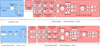 |
Fig. 1 Block diagrams of the receivers (one detector). Top: 30-GHz Instrument. Bottom: 40-GHz Instrument. The diagram is taken from Artal et al. (2020). |
3 Ground calibration
3.1 Setup
The calibration process involves positioning the so-called multi-frequency calibration instrument (MFCI) in front of the detector and acquiring calibration data, as illustrated in Fig. 2. The MFCI consists of two feedhorns and OMTs, similar to the cryogenically cooled feedhorns and OMTs of the TFGI, and is connected back-to-back through two identical −20 dB waveguide couplers. The calibration signal is introduced through one coupler, while the other is terminated with a room-temperature load. The horns are aligned through a concentric stepper motor axial drive, and this setup is designed to be attached to a detector-centered polarization grid known as a fixed plate. Additionally, a tilted aluminum flat mirror points the horn arrangement toward the sky when the cryostat is mounted on the focal plane of the QT2. In this way, the background radiation during a calibration run comes from the sky. The injected signal corresponds to the diode’s equivalent temperature when ON with a 20 dB coupling ratio. A wideband noise diode (Keysight 346CK011) was selected for its coverage of both FGI and TGI bands.
For installation, the MFCI is preassembled horizontally using a digital inclinometer and mounted onto the telescope focal plane with 0.2 deg mechanical repeatability of the MFCI mounting angle when reinstalling the calibration plate. A dedicated acquisition system controls the stepper motor, the diode, and the phase switches. Polarization angles are referenced with respect to the diode’s E-field and defined as positive for anticlockwise rotation from the sky toward the instrument. The alignment plate is secured over the cryostat focal plane, and the MFCI is attached with spring-loaded clamps, ensuring the mirror maintains its skyward orientation. Electrical connections for the motor, diode, and switches are routed through dedicated cabling.
The 16 possible states of the phase switchers could present a misalignment with respect to the desired angle (0, 90, 180, and 270 deg). Due to their non-idealities, deviations from the expected polar measurement occur. However, due to the complete coverage of all phase errors, any systematic error is generally canceled when all states are summed with the correct error for a given Stokes parameter. Notwithstanding, we want to prove this and characterize the precision of such an instrumental defect, in Sect. 3.6.
Process of polarization characterization and mathematical framework. Each phase switch is designed to introduce a phase shift as close as possible to its nominal value – either 90 deg or 180 deg. However, imperfections in the hardware can lead to small deviations, denoted as ϵ, from the nominal phase shift, and may also introduce frequency-dependent variations across the band. These deviations must be carefully characterized and, if necessary, corrected to ensure accurate signal reconstruction and minimize systematic errors. In principle, averaging over the four equivalent engineering states to produce a science state (see Sect. 2) can help reduce the impact of phase errors, assuming that the errors are random. However, a residual systematic contribution may remain, particularly if the phase error exhibits some degree of coherence or bias across states.
To break the degeneracies between the phase error (ϵ) and other instrument-induced angles, we built a dataset where the polarization angle of the calibration source is rotated by an angle γ, by a polarizer. This polarizer introduces an angle that allows us to repeat the same measurement with a controlled shift. The values for γ range from −45.0 to 67.5 deg in steps of 22.5 deg, (−45.0, −22.5, 0.0, 22.5, 45, and 67.5 deg). This approach yields six measurements for each phase state, thereby adding five equations to the system for each fixed phase state. Mathematically, in a simplified form where the incoming light is assumed to be fully polarized, we can express the Stokes-parameters equations as
![Mathematical equation: $\[\begin{aligned}& P=\sqrt{Q^2+U^2}=I \\& Q=P \cdot \cos \left[2\left(\gamma-\phi_c\right)\right] \\& U=-P \cdot \sin \left[2\left(\gamma-\phi_c\right)\right],\end{aligned}\]$](/articles/aa/full_html/2026/04/aa58376-25/aa58376-25-eq1.png) (1)
(1)
where I, Q, and U represent the Stokes parameters; γ is the polarization angle of the calibration source; and ϕc is the reference polarization angle of the TFGI polarimeter. The minus sign in U is due to the instrument’s coordinate frame: The TFGI reference axis is mirrored relative to the standard sky-frame definition, which flips the sign of the measured U component. Introducing Eq. (1) into the set of equations that define the TFGI channels’ responses produces a new set of equations that relate the output of each channel to the input Stokes parameters. Consequently, the simplified (see Fernández-Torreiro 2023 for the extended formalism) TFGI equations – in the assumption of 100%-polarized signal – for the TGI and FGI channels (output voltages of each detector or polarimeter), respectively (distinguished in the superscript), are
![Mathematical equation: $\[\mathrm{V}_{1,4}^{\mathrm{TGI}, \mathrm{FGI}}=\frac{1}{2} g_{1,4} I\left[1-\eta ~\sin~ \left[\delta+\epsilon_{1,4}(\delta)+2\left(\gamma-\phi_{\mathrm{c}; 1,4}\right)\right]\right]\]$](/articles/aa/full_html/2026/04/aa58376-25/aa58376-25-eq2.png) (2a)
(2a)
![Mathematical equation: $\[\mathrm{V}_{2,3}^{\mathrm{TGI}, \mathrm{FGI}}=\frac{1}{2} g_{2,3} I\left[1+\eta ~\sin~ \left[\delta+\epsilon_{2,3}(\delta)+2\left(\gamma-\phi_{\mathrm{c}; 2,3}\right)\right]\right]\]$](/articles/aa/full_html/2026/04/aa58376-25/aa58376-25-eq3.png) (2b)
(2b)
![Mathematical equation: $\[\mathrm{V}_{3,1}^{\mathrm{TGI}, \mathrm{FGI}}=\frac{1}{2} g_{3,1} I\left[1+\eta ~\cos~ \left[\delta+\epsilon_{3,1}(\delta)+2\left(\gamma-\phi_{\mathrm{c}; 3,1}\right)\right]\right]\]$](/articles/aa/full_html/2026/04/aa58376-25/aa58376-25-eq4.png) (2c)
(2c)
![Mathematical equation: $\[\mathrm{V}_{4,2}^{\mathrm{TGI}, \mathrm{FGI}}=\frac{1}{2} g_{4,2} I\left[1-\eta ~\cos~ \left[\delta+\epsilon_{4,2}(\delta)+2\left(\gamma-\phi_{\mathrm{c}; 4,2}\right)\right]\right].\]$](/articles/aa/full_html/2026/04/aa58376-25/aa58376-25-eq5.png) (2d)
(2d)
Here, V is the output in volts2, g is the gain, η is the polarization efficiency, δ is the phase state of each polarization state (0, 90, 180, and 270 deg), and ϵ is the correction angle that represents the deviation from the nominal phase value assumed constant over the band. The subscript indicates the channel, with a comma distinguishing between TGI and FGI. Also g, ϵ, and ϕc differ between TGI and FGI. Operationally, we used Eq. (2c) for all channels in the on-sky analysis since the four-channel equations are mathematically equivalent and differ only by successive 45-degree rotations. Therefore, adopting a single convention simplifies the on-sky data processing without loss of generality.
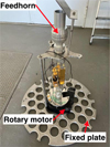 |
Fig. 2 Photo of the MFCI mounted on the calibration alignment plate. The diode used introduces the known signal into the TFGI detectors. The fixed plate is placed on top of the focal plane and defines the different detector locations where the diode can be positioned. The rotary motor allows for the modification of the calibration diode’s orientation (γ) in 22.5 deg steps to study different linear polarization inputs. A detailed description is presented in Fernández-Torreiro (2023). |
3.2 Data
As outlined in Sect. 3.1, the calibration tests involve assessing the signal response while manipulating the angle of a polarizer placed between the feedhorns of the polarimeters and the calibration source. Initially, the diode source is activated (these data are referred to as diode ON). Subsequently, the source is deactivated (these data are referred to as diode OFF) to measure the background signal. Figure 3 displays an example of a complete block of data (~8 ms), where the first part presents the diode signal (diode ON) and the right part represents the pure background signal (diode OFF). The steps indicate the different 16 phase states, and the colors identify the channels. The outputs from the different channels vary at different levels due to the varying gains of the system, which we characterize in Sect. 3.4.
By averaging the blocks for each phase state, we computed the pure diode signal (Vdiode) as
![Mathematical equation: $\[\mathrm{V}_{\text {diode }}=\mathrm{V}_{\mathrm{ON}}-\mathrm{V}_{\mathrm{OFF}},\]$](/articles/aa/full_html/2026/04/aa58376-25/aa58376-25-eq6.png) (3)
(3)
where VON is the diode ON signal (left side of Fig. 3) and VOFF is the diode OFF signal (right side of Fig. 3). We first utilized a straightforward dataset for TGI where the external polarizer is not included (i.e., no γ angle), named Pixel23_2022_April_06_0. This more straightforward dataset was used to assess the data quality, as reported in the next paragraph, concerning response saturation and stability over time. Finally, for the ϵ characterization, we concentrated on three specific datasets where we introduced the external polarizer (with γ angles of −45.0, −22.5, 0.0, 22.5, 45, and 67.5 deg): Pixel23_2022_April_06_1, Pixel23_2022_April_ 06_2, and Pixel23_2022_April_07_3. The visualization of the data structure is present in Appendix B.
Data assessment with diode reference: Response saturation and stability in the time stream. Data assessment is crucial for ensuring the reliability and accuracy of the scientific results derived from observations. This process involves carefully scrutinizing the raw data collected by the instrument, identifying potential artifacts or noise sources, and implementing corrective measures to reduce their impact on the final analysis.
First, we evaluated the quality of the data by visually inspecting the time-ordered information. As expected, the signal reaches its maximum value at 10 V. However, a nonlinear response could occur before reaching this threshold, resulting in a loss of information on one side and introducing systematic effects in the response evaluation on the other. We observed high signal levels in the diode ON reference data, indicating the presence of saturation-related systematics. In contrast, the signal in the diode OFF reference is significantly lower (see Fig. 3). We do not modify or correct the signal in the presence of saturation in this work.
The next critical step involves assessing the stability of the data, which refers to the system’s ability to consistently translate the same incoming signal into the same electric (readout) signal across different instances. The total measurement duration spans 1 minute. To evaluate stability, we resampled each phase state (comprising 40 points each at a sampling rate of 160 kHz) by calculating their averages. Subsequently, we plotted the time series of these averages and applied linear regression to determine the slope. A slope close to zero indicates a stable output signal.
We performed a statistical analysis of response stability. Across all channels and phase states, the signal is consistently reproduced throughout the 1-minute duration, showing no noticeable drift or instability. The “diode ON” data corresponds to the activation of the input calibration signal. In contrast, the “diode OFF” data were collected when the reference source is off and the detector registers the background. The results are shown in Fig. 4.
The data present a linear regression slope of a few hundred millivolts per minute; −1.6 ± 0.8 mV/min in the diode ON case and −2.5 ± 0.3 mV/minute in the diode OFF case. The uncertainties are calculated as the standard deviation of the counts. This leads to a drift in the signal smaller than 2 mV in a minute. Equivalent to ~50 mK by applying the average on-sky responsivity reported in Sect. 5.2. This instability is likely due to a combination of gain drift and the instability of the optical load, originating from the background and the diode. Although this small drift is detectable, it has a negligible impact on the results discussed here. Firstly, it is comparable to the white-noise level. Secondly, it is subdominant with respect to other systematic effects in the calibration. In particular, differences between the four phase-state configurations, which should nominally produce identical values, dominate the uncertainty budget at the few-percent level, whereas the measured drift over one minute is only at the millipercent level.
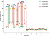 |
Fig. 3 Example of a full data block, ~8 ms. The left part of the voltage output shows the diode “ON”, while the right part shows the diode “OFF”. Each color identifies a channel output. The signal exhibits saturation, reaching a value of 10 V, in some cases. |
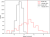 |
Fig. 4 Histogram of the slopes that quantify the signal stability in a data acquisition of 1 minute. Each count is defined as a function of the slope obtained from linear fitting. The slope values span a range of ~ −2.5–0.5 mV/min for the diode ON case, indicating a lack of significant stability issues within 1 minute of integration. |
3.3 Polarization efficiency calibration
The polarization efficiency of a system quantifies how effectively the instrument produces, transmits, or manipulates polarized light. Polarization efficiency depends on several factors. First, high-quality polarizing elements block or transmit light based on its orientation. Accurate alignment of optical components within the system is crucial to prevent polarization distortion or loss. Additionally, the properties of the materials used in optical components affect polarization characteristics. Efficiency may vary across the electromagnetic spectrum, which can impact system performance. Environmental conditions, such as temperature and humidity, can influence polarizing elements and polarization efficiency. Finally, system design, including component arrangement and the choice of elements, is essential for optimizing efficiency and minimizing unwanted polarization effects. Quantifying polarization efficiency involves measuring the degree of polarization of light at different stages of the system and comparing it to the input (see Tinbergen 1996 for a detailed description of light polarization). In the TFGI case, the frequency dependence of polarization efficiency on wavelength is not fully appreciated, as it is integrated across the bandpass. Since the calibration signal is fully polarized, the polarization efficiency is expressed as ![Mathematical equation: $\[\eta=\sqrt{Q^{2}+U^{2}} / I\]$](/articles/aa/full_html/2026/04/aa58376-25/aa58376-25-eq7.png) , where we can obtain the I Stokes parameter from Eq. (2) as
, where we can obtain the I Stokes parameter from Eq. (2) as
![Mathematical equation: $\[I=[\mathrm{V}(0 \text { deg })+\mathrm{V}(90 \text { deg })+\mathrm{V}(180 \text { deg })+\mathrm{V}(270 \text { deg })] / 2,\]$](/articles/aa/full_html/2026/04/aa58376-25/aa58376-25-eq8.png) (4)
(4)
where the angle values in the brackets correspond to δ, and the Q and U Stokes parameters are defined in Appendix C for all the sets of equations. We utilized the voltage output of a pure diode signal (Vdiode) by calculating it with Eq. (3). We conducted statistical analyses for each channel and polarizing angle (γ), alongside the three selected datasets, to calculate the polarization efficiency in percentage (η). The average results are presented at the top of Table 1. The uncertainty was calculated through the standard deviation across different datasets. A detailed report is provided in Table C.1.
The system exhibits a mean polarization efficiency across the channels of η = 95 ± 2%, indicating a polarization loss3 of under ~10%. The uncertainty of the mean polarization efficiency is determined as the standard deviation across the value per channel. The extensive results, presented by polarizing angle and dataset, are reported in Table C.1 of the Appendix C. These values are comparable to the Multi-Frequency Instrument (MFI) values (Table 6 in Rubiño-Martín et al. 2023).
Characterization of Pixel 23 from ground measurements.
3.4 Responsivity calibration
We utilize the dataset Pixel23_2022_April_06_0 to characterize the responsivity of Pixel 23. The dataset comprises repetitive blocks of the diode calibrator in both the ON and OFF states, enabling the subtraction of the background from the pure signal of the calibrator. By construction, we know that the diode emits 600 ± 40 K, with uncertainty introduced by the diode switcher (0.1 dB, which is a Sage SKQ-01 attenuator featuring up to 2.5 dB insertion loss) and the diode itself (0.2 dB). The results for each channel are presented in the second row of Table 1. The uncertainty is calculated by propagating the uncertainties of the output voltages and the diode temperature in the calculation of responsivity.
The responsivity calculated from the diode is primarily affected by the uncertainty in the diode’s emitted power as seen by the detector, and the fact that this measurement does not reflect the actual observational configuration used on-sky – for instance, it does not include coupling through the QT2 mirrors, which alters the beam pattern and effective system gain. While the detector’s intrinsic responsivity should, in principle, be independent of the optical setup, the total optical coupling efficiency and beam gain introduced by the optics do influence the system-level responsivity. Additionally, the relatively high temperature of the diode may induce nonlinearities in the detector response, further complicating the calibration. The calibration diode is mainly used to monitor system responsivity stability rather than to provide an absolute responsivity calibration. However, future measurements will incorporate active thermal control and a lower-output diode to further mitigate possible nonlinear effects.
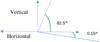 |
Fig. 5 Schematic of the polarization angle measurement of the telescope. The axes represent the ground tilt (Horizontal) and the deviation from zenith (Vertical). |
3.5 Polarization angle calibration
The reference polarization angle of the channels, ϕc, determines the relation between the measured Stokes Q and U parameters and those associated with the incoming radiation field measured on the Az-El QT2 reference frame.
For this measurement, the zero polarization angle (see Tinbergen 1996 for a detailed description) of the entire system for TGI (measured from the MFCI encoder home position), taking into account the telescope (calculating the angle with respect to the vertical) and considering ϵ = 0 deg, was found to be
![Mathematical equation: $\[{\mathrm{pol} \_\mathrm{ang}_{\mathrm{TGI}}}=82.5 ~\mathrm{deg}+0.15 ~\mathrm{deg}-90.0 ~\mathrm{deg}=-7.35 ~\mathrm{deg}.\]$](/articles/aa/full_html/2026/04/aa58376-25/aa58376-25-eq9.png) (5)
(5)
Figure 5 illustrates the schematic of the zero polarization angle of the telescope, where 0.15 deg is the horizontal (ground) tilt found when measuring the angle of the fixed plate horizontally of the telescope. Note that the angles are measured from the horizontal, as a digital inclinometer was utilized, and then referred to the vertical in the equation by subtracting 90 deg. The double of the resulting angle (pol_angTGI = −7.35 deg) was then applied to the measurement with diode reference for comparison to the one calculated from astrophysical sources as
![Mathematical equation: $\[\phi_{\mathrm{c}}=\gamma_{\mathrm{ref}}-2 \text { pol_ang}_{\mathrm{TGI}},\]$](/articles/aa/full_html/2026/04/aa58376-25/aa58376-25-eq10.png) (6)
(6)
where γref is the polarization angle computed in the instrument reference.
Once the telescope’s zero polarization angle was calculated, we proceeded to characterize the polarization angle using the diode for each channel. The data used for this calculation are the same as described at the beginning of this section. We calculated the polarization angle as
![Mathematical equation: $\[\phi_{\mathrm{c}}=\frac{1}{2} ~\arctan~ \left(\frac{-U}{Q}\right)-2 \text { pol }_{-} \text {ang}_{\mathrm{TGI}},\]$](/articles/aa/full_html/2026/04/aa58376-25/aa58376-25-eq11.png) (7)
(7)
where U and Q are the Stokes parameters computed with the linear combination of the outputs (V) with the equations reported in Appendix C. Table 1 reports the calculated polarization angle for each channel using Eq. (7). The uncertainty is calculated across the different datasets as the standard deviation. A detailed report is provided in Table D.1.
The difference between polarization angles calculated for consecutive channels is ~48±9 deg. This is consistent with the expected value of 45 deg (note that, as mentioned before, we apply Eq. (2c) for all four channels). The uncertainty (±9 deg) is calculated as the standard deviation of the pairwise angular differences, with each channel matched to the nearest other angle in the set. Since the single-angle uncertainty is much smaller, this 9-degree angle seems to correspond to real differences in the angle between channels rather than to a statistical uncertainty. Appendix D describes the polarization angles for each channel, polarizer angle (γ), and dataset reported in Table D.1. The results in Table 1 can be compared to those in Table 2, which were obtained using an alternative fitting method explained in the following section.
Fit polarization angle (ϕc).
3.6 Calibration of phase errors
To improve the polarization angle reconstruction, we aimed to characterize the phase-switch error angles, ϵ, and use them to correct the TFGI equations. For this purpose, we addressed a three-parameter problem (gI4, ϵ, ϕc) with six equations corresponding to the six values of γ for each channel and phase state. In this study, we considered a distinct ϕc for each channel. The fitting process unfolded in two phases. Initially, we fit the data to Eq. (2) to obtain ϕc and gI for each channel without considering any ϵ correction. Subsequently, with ϕc and gI fixed from the previous step, we reintroduced ϵ into the equations for each channel and phase state.
ϕc fitting. The initial fitting step was aimed at constraining the ϕc parameter for each channel. We fit Eq. (2c) under the assumption of ϵ = 0 deg. Consequently, the resulting ϕc values encompass the average ϵ across different phase angles. Subsequently, we performed the fitting for each dataset, with 19, 15, and 15 iterations, respectively, for the three datasets. We exploited the results reported in Table 1 (last row) as the initial guess of the fitting for ϕc. The results are reported in Table 2.
The fitting step converges into reference angles for each channel with ~0.6-deg precision, and the final values are compatible at the 2-σ level with the initial values reported in Table 1.
ϵ fitting. We conduct fitting of Eq. (2) while maintaining the ϕc fixed for each channel, as determined in Sect. 3.6. This fitting process is carried out individually for each dataset. In conclusion, we undertake a statistical analysis by calculating the average values and their corresponding standard deviations across the three datasets. The results are presented in Table 3.
The results are compatible with the null value at the 2σ level, where σ=0.65 deg corresponds to the mean uncertainty of the mean phase-error values reported in the last row of Table 3, which have an average value of 1.3 deg. Therefore, we do not need to consider any corrections for scientific purposes at a ~1-degree precision, which is the specification for the TFGI for the polarization angle. The datasets exploited for the ϵ calculation are recorded with a separation of ~18 hours. The ambient variables, particularly temperature, may have influenced the response of the phase switches. More datasets at lower timescale differences might be helpful for future development. The determination of phase-switch errors relies on a nonlinear fitting process and can, in theory, depend on the choice of initial parameters or converge to local minima. In practice, incorrect solutions are easily identified through visual inspection of the fit modulation patterns. Additionally, for data of poor quality, the fit fails to converge to a physically meaningful solution, providing a clear diagnostic for excluding unreliable measurements. These checks help prevent biases when estimating the phase-switch errors. Appendix E presents the results per dataset.
Phase error corrections (ϵ).
4 On-sky calibration
After calibrating the instrument using the diode reference on the ground (as described in the previous section), we characterize the instrument with astrophysical sources. We perform various observing tests during the instrument’s commissioning phase, employing observations of Tau A (see Sect. 4.1) and the Moon (see Sect. 4.2) to characterize TGI Pixel 23. The following sections detail the calibration methods used and present the respective results, which will be compared across all methods and calibration sources studied in this work in Sect. 5.
4.1 Tau A
4.1.1 Polarization efficiency with Tau A
We used Tau A observations to estimate the polarization efficiency similarly to that described in Section 3.3. Tau A has been extensively used for this purpose in the past (e.g., Rubiño-Martín et al. 2023) thanks to being very bright at radio-to-microwave frequencies (>300 Jy at frequencies <10 GHz). It presents a high polarization fraction, being ~7% at frequencies >10 GHz (e.g., Ritacco et al. 2018).
For this analysis, we selected the Tau A observation with the best noise properties while being close in time to the Moon observation discussed in Sect. 4.2. This observation consists of a single raster scan, and its properties are summarized in Table 4. From this observation, we produce maps of the three Stokes parameters for each channel independently, which are shown in Fig. 6. The detection of a polarized signal from Tau A is immediately clear. To estimate the source flux density, we use a beam-fitting (BF) photometry that involves fitting the I, Q, and U maps of each channel to a 2D Gaussian with fixed position (using the nominal coordinates of Tau A) and width fixed to the FWHM of the beam calculated in Fernández Torreiro et al. (in prep.). The amplitudes of the Gaussians obtained from these fits define IBF, QBF and UBF estimates, with their uncertainties being σ(IBF), σ(QBF) and σ(UBF). At the TFGI angular resolution, Tau A is only marginally resolved and is therefore well described by a Gaussian profile; any residual source-extension effects are absorbed into the BF uncertainty. As a consistency check, we also performed aperture photometry on the Tau A observations and obtained results consistent with the BF analysis.
Polarized intensity, P, maps in Fig. 6 are calculated as ![Mathematical equation: $\[\sqrt{Q^{2}+U^{2}}\]$](/articles/aa/full_html/2026/04/aa58376-25/aa58376-25-eq12.png) for visualization purposes. However, the estimates for P used to compute the polarization efficiency are not directly derived from the P maps; rather, they come from the Q and U BF estimates, QBF and UBF. We divide this P by the fit IBG and compare the result with the model. This approach minimizes the noise bias that affects polarized intensity measurements in regions with low signal-to-noise ratios.
for visualization purposes. However, the estimates for P used to compute the polarization efficiency are not directly derived from the P maps; rather, they come from the Q and U BF estimates, QBF and UBF. We divide this P by the fit IBG and compare the result with the model. This approach minimizes the noise bias that affects polarized intensity measurements in regions with low signal-to-noise ratios.
We used the ratio of the measured polarization fraction to the expected value from previous measurements to estimate the polarization efficiency of our detectors. We assumed the expected value would be constant and equal to 7 ± 0.1% at TFGI frequencies. We obtained this value from the weighted average of the results for the five frequency bands given in Weiland et al. (2011). Although the FWHM values in Weiland et al. (2011) bands are larger than the one from TFGI, the signal from Tau A is fully contained in one beam in both cases. Because of that, we do not expect a change in the polarization fraction, as shown by previous works (see, e.g., Fig. 39 from Rubiño-Martín et al. 2023). We did not propagate this 0.1% uncertainty to the final map measurements, as the errors in IQU measurements dominate. We find an average polarization efficiency across the channels of η = 95 ± 3% (the uncertainty is calculated as the standard deviation across the channels), with a single-channel efficiency between η ~ 91–98% (as seen in Table 4).
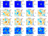 |
Fig. 6 Maps of the single Tau A observation used to estimate polarization efficiency, smoothed at 1 deg. We discuss in Sect. 4.1.3 how these uncalibrated maps are utilized to calculate the polarization angle. From top to bottom, the rows show the Stokes parameters I, Q, U, and polarized intensity P. From left to right, the columns show channels 1, 2, 3, and 4. |
Raster scan observation properties and characterization of Pixel 23 with Tau A.
4.1.2 Responsivity calibration with Tau A
We compared the estimates obtained in the previous section with BF with the expected values derived from the Tau A model presented in Rubiño-Martín et al. (2023) in order to estimate its responsivity:
![Mathematical equation: $\[S_\nu=358.3 ~\mathrm{Jy}\left(\frac{v}{22.8 ~\mathrm{GHz}}\right)^{-0.297}.\]$](/articles/aa/full_html/2026/04/aa58376-25/aa58376-25-eq13.png) (8)
(8)
We applied the −0.21% year−1 secular decrease value from Weiland et al. (2011), using t0 = 2016.3 year as the reference time for the model and t = 2021.9 year for the observation.5 The expected flux is therefore S31 GHz = 323.23 Jy. We converted this S31 GHz into temperature as follows6:
![Mathematical equation: $\[T_\nu=S_\nu\left(\frac{2 k_{\mathrm{B}} \nu^2}{c^2} \Omega_b\right)^{-1},\]$](/articles/aa/full_html/2026/04/aa58376-25/aa58376-25-eq14.png) (9)
(9)
where Ωb is the solid angle subtended by the model beam, Ωb = 4.77 × 10⁻⁵ sr. The expected temperature at 31 GHz is then 230 mK. We obtained the responsivity by dividing the amplitude calculated through BF photometry on the intensity map, IBF, by the calculated temperature. We report the responsivities derived from Tau A in Table 4 (for the single raster scan described in the previous section). We also calculated the responsivity values for the coadded monthly maps (from Fernández-Torreiro et al., in prep.) from November 2021, December 2021, and January 2022. We report the responsivities derived from Tau A in Tables 4 (for the single raster scan described in the previous section) and 5 (for the monthly coadded maps). We also computed the responsivity from Moon observations, as discussed in the following Section. We present this sky-sky check of the responsivity in Sect. 5.2.
4.1.3 Polarization angle
We computed the reference polarization angle from the comparison between the one calculated from our raw on-sky data, γ′, and the expected one, γTauA:
![Mathematical equation: $\[\phi_c=\gamma_{\mathrm{TauA}}-\gamma^{\prime}=\gamma_0+\mathrm{RM} \lambda^2-\frac{1}{2} ~\arctan \left(\frac{-U}{Q}\right),\]$](/articles/aa/full_html/2026/04/aa58376-25/aa58376-25-eq15.png) (10)
(10)
where γ0 = −88.31 ± 0.25 deg and RM = −1406 ± 12 deg m−2 is the rotation measure (Rubiño-Martín et al. 2023). Additionally, the minus sign for γ′ represents the change in the x-axis direction when transitioning from the telescope to the sky coordinate system.
We computed ϕc from QBF and UBF values from Sect. 4.1.1 using Eq. (10). We summarize the results in Table 6. Finally, we estimated the uncertainties of ϕc by drawing 10 000 random realizations for Q and U distributions. We defined these distributions as Gaussians with centers equal to QBF and UBF and standard deviations equal to σ(QBF) and σ(UBF). We evaluated ϕc for each pair QBF − UBF and then built its distribution. We defined the uncertainty on ϕc as the width of such a distribution.
Responsivity (ℜ) characterization with Tau A.
Polarization angle (ϕc) characterization with Tau A.
4.2 The Moon
We use three Moon observations to characterize TGI Pixel 23 in the sky. These observations were performed on 21 November 2021, 28 December 2021, and 23 January 2022. Each observation involves repeated azimuth slews (azimuth scans at fixed elevation) lasting ~1 hour, covering an azimuth range of 100 deg at a speed of 4.5 deg/s. The azimuth scan spans 100 deg to ensure full beam crossing for all pixels, thereby minimizing edge effects and ensuring uniform beam sampling.
4.2.1 Moon emission model
Moon’s polarized microwave emission is produced mainly by its own thermal emission. Its brightness temperature can be modeled, following Hafez et al. (2014), as
![Mathematical equation: $\[T_{\text {Moon}}=T_0(\nu)+T_1(\nu) \cos (\phi(t)-\xi(\nu)),\]$](/articles/aa/full_html/2026/04/aa58376-25/aa58376-25-eq16.png) (11)
(11)
where T0 represents the mean temperature and T1 is the amplitude of the temperature variation associated with the Moon’s phase, ϕ(t). Finally, ξ(ν) is the phase relative to the time of the full Moon. The values at 31 GHz for these parameters are interpolated from the values presented in Hafez et al. (2014), obtaining: T0(31 GHz) = 213.3 ± 0.9 K, T1(31 GHz) = 35 ± 2 K ξ(31 GHz) = 28 ± 4 deg. For our three observing dates (21 November 2021, 28 December 2021, and 23 January 2022), the corresponding lunar phases are ϕ=19.4 deg, 104.4 deg, and 60.2 deg, respectively. In this work, we do not include spatial dependence on the thermal signal due to the low angular resolution of the telescope, and it is not expected to significantly affect either the absolute signal (at most ~8% discrepancy with Zheng et al. 2012 model in these dates) or the polarization morphology. Additionally, our observations were made relatively near the time of the full Moon, which also decreases the contribution of spatial anisotropies.
Additionally, the modeling of polarized emission is feasible, as it is only weakly polarized because of the refraction of thermal radiation on the Moon’s surface. Following Fresnel equations (see, e.g., Born & Wolf 1959), the transmittances of the perpendicular t⊥ and the parallel t∥ components were defined as follows:
![Mathematical equation: $\[\begin{aligned}t_{\perp} & =\frac{2 n_{\text {Moon}} ~\cos~ \theta_i}{n_{\text {Moon}} ~\cos~ \theta_i+n_t ~\cos~ \theta_t}, \\t_{\|} & =\frac{2 n_{\text {Moon}} ~\cos~ \theta_i}{n_t ~\cos~ \theta_i+n_{\text {Moon}} ~\cos~ \theta_t},\end{aligned}\]$](/articles/aa/full_html/2026/04/aa58376-25/aa58376-25-eq17.png) (12)
(12)
where nMoon is the refraction index of the Moon, nt is the refraction index of the free space (nt ≈ 1), and θi and θt are the incident and transmitted angles, respectively. To better understand these angles, we refer to Fig. 7, from which we derived the relation θt = arcsin (r′/R), where r′ is the radial coordinate and R is the radius of the Moon.
By exploiting the transmittance values described in Eq. (12), we calculated the intensity (IMoon) and the polarization (PMoon) of the Moon’s surface as a function of its temperature (TMoon):
![Mathematical equation: $\[\begin{aligned}I_{\text {Moon }} & =\frac{T_{\text {Moon }}}{2}\left(t_{\|}^2+t_{\perp}^2\right) \frac{\partial \theta_i}{\partial \theta_t}, \\P_{\text {Moon }} & =\frac{T_{\text {Moon }}}{2}\left(t_{\|}^2-t_{\perp}^2\right) \frac{\partial \theta_i}{\partial \theta_t},\end{aligned}\]$](/articles/aa/full_html/2026/04/aa58376-25/aa58376-25-eq18.png) (13)
(13)
where the term ∂θi/∂θt describes the change in the solid angle of the incident beam after the refraction process.
By solving these equations, we obtained the radial intensity and polarization patterns for the Moon’s emission. We note that the polarization direction is parallel to the radial direction, and it thus has rotational symmetry. Therefore, if we consider that in a reference frame centered on the Moon, the polarization signal is entirely contained in the Stokes Q parameter, we can estimate the Stokes parameters Qp, Up of a given pixel (p) by applying the following rotation:
![Mathematical equation: $\[\binom{Q_p}{U_p}=\left(\begin{array}{cc}\cos~ 2 \varphi_p & -\sin~ 2 \varphi_p \\\sin~ 2 \varphi_p & \cos~ 2 \varphi_p\end{array}\right)\binom{P_{\text {Moon,} \mathrm{p}}}{0},\]$](/articles/aa/full_html/2026/04/aa58376-25/aa58376-25-eq19.png) (14)
(14)
where φp is the polar angle that gives the orientation of the pixel p with respect to the map axis (northeast direction). Thus, using this model, we can obtain the Stokes parameters in the northeast Moon-centered coordinate frame and the total polarization intensity ![Mathematical equation: $\[P_{\text {tot}}=\sqrt{Q^{2}+U^{2}}\]$](/articles/aa/full_html/2026/04/aa58376-25/aa58376-25-eq20.png) as a function of TMoon and nMoon.
as a function of TMoon and nMoon.
Finally, to compare the model with the measured data and calibrate the various parameters of our instrument, we also need to consider the beam shape of our instrument. First, we convolve the modeled maps with a Gaussian beam with the TGI’s FWHM (21 arcmin). After that, as described in Sect. 4.2.4, we find the relative angle that gives the best fit between the model and the data. Figure 8 displays both the observed (left) and simulated (right) maps using a fixed refraction index nMoon = 1.22 (from Losovskii 1967 at 37 GHz), after applying all the corrections (for a detailed description of this model; see, e.g., Bischoff 2010; Perley & Butler 2013; Xu et al. 2020; Dahal et al. 2023).
As in Xu et al. (2020), we did not observe the emergence of the quadrupolar polarization pattern in a single observation of the Moon for the central detector. In this work, we assumed a uniform temperature, TMoon, across the lunar disk, thereby simplifying the latitude-dependent model proposed by Zheng et al. (2012). Even after including the latitude-dependent model and stacking the three available maps taken at different epochs and incorporating the latitude-dependent temperature model, the quadrupolar pattern is not recovered in Pixel 23 (central pixel). The behavior is repeatable and stable over the timescale of our observations (~2 months). In contrast, the quadrupolar structure is clearly visible in single observations from other TFGI detectors. We performed preliminary simulations and tests to investigate potential explanations, including intensity-to-polarization leakage, nonlinear response, saturation effects, phase state angle misestimation, and mapping strategy artifacts. None of these effects explains the observed behavior. Therefore, the origin of this discrepancy for the central detector remains unclear. Even when the quadrupolar pattern is only partially visible (i.e., one lobe is missing), the relative orientation between the polarization patterns observed in Stokes Q and U is preserved. Since the polarization angle determination relies on these relative rotations rather than on the full quadrupolar morphology, the measurements still provide a robust estimate of the polarization angle. A dedicated future study will address this issue in detail, including a comprehensive analysis of Moon observations across all TFGI detectors, once the instrument is installed again on the focal plane of QT2. The TFGI instrument was temporarily removed after the initial commissioning phase. A new configuration comprising 19 receivers (10 at 31 GHz and 9 at 41 GHz) is being prepared, and observations are expected to resume in spring 2026.
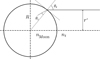 |
Fig. 7 Schematic describing the Moon’s emission model and the parameters involved: the refraction index of the Moon (nMoon), the refraction index of free space (nt), the incident (θi) and transmitted (θt) angles, the radial coordinate (r′), and the radius of the Moon (R). |
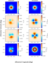 |
Fig. 8 Moon maps of the three Stokes parameters I, Q, and U and of the polarized intensity P for an observation taken on December 2021 (left) and for the simulated model inferred from the observation parameters (right). |
Polarization efficiencies (η) with the Moon.
4.2.2 Polarization efficiency with the Moon
We recovered the polarization efficiency by comparing the polarization fractions obtained from the measurements with those from the modeled signal. The modeled polarization fraction depends tightly on the refraction index of the Moon, nMoon, which has not been directly measured with the required precision to date at 31 GHz.
In a first attempt, we derived an estimate of the polarization efficiency as η = Pobs/Pmod, where ![Mathematical equation: $\[P_{i}=\sqrt{Q_{i}^{2}+U_{i}^{2}} / I_{i}\]$](/articles/aa/full_html/2026/04/aa58376-25/aa58376-25-eq21.png) and Qi, Ui, and Ii are the flux densities calculated through an aperture photometry (AP) technique with a radius of 48 arcmin on the corresponding maps resulting from the observation data (i=obs) or from the model (i=mod). We assumed a value of the refraction index nMoon = 1.22 (from Losovskii 1967) and obtained the results reported in Table 7 for each channel and for each observation. The mean polarization efficiency across channels and observations is η = 89 ± 2%, with the uncertainty calculated as the standard deviation across the mean values for each channel.
and Qi, Ui, and Ii are the flux densities calculated through an aperture photometry (AP) technique with a radius of 48 arcmin on the corresponding maps resulting from the observation data (i=obs) or from the model (i=mod). We assumed a value of the refraction index nMoon = 1.22 (from Losovskii 1967) and obtained the results reported in Table 7 for each channel and for each observation. The mean polarization efficiency across channels and observations is η = 89 ± 2%, with the uncertainty calculated as the standard deviation across the mean values for each channel.
It is important to note at this point that the uncertainty on the polarization efficiency recovered value is mainly dominated by the uncertainty on the refraction index, which has been set as 0.05. Given the difficulty of assessing the exact value of nMoon, and of its uncertainty, due to the lack of measurements in this frequency range, we have decided to invert the problem and derive a value of nMoon from our observations by fixing the polarization efficiency to the values derived from Tau A shown in Table 4. This approach, which is presented in Appendix A, yields an effective refraction index of nMoon = 1.209 ± 0.007 (stat) ± 0.009 (sys), compatible at ~1σ with the value constrained by Losovskii (1967).
Responsivity (ℜ) with the Moon.
4.2.3 Responsivity calibration with the Moon
We calculated the Moon’s brightness temperature from Eq. (11). Thus, we could model the thermal emission of the Moon at 31 GHz on different dates (Moon phases) and simulate, similar to the previous sections, emission maps that we directly compare with the observations. We performed an AP study on both simulated and measured maps in intensity (e.g., as in the first row of Fig. 8) and compared them to determine the detector’s responsivity. The calculated responsivities for Pixel 23 are reported in Table 8. We compared the Moon and Tau A results in Sect. 5.2.
4.2.4 Polarization angle
The polarized emission of the Moon exhibits a characteristic quadrupolar pattern, as illustrated in the model shown on the right of Fig. 8. When observed with sufficient angular resolution to resolve this structure, the polarization angle of the detectors (ϕc) can be determined by fitting the real data to the model. Specifically, the Stokes parameters measured by the instrument (Qobs and Uobs) are related to the modeled Stokes parameters (Q and U) through a rotation by an angle of 2ϕc, as
![Mathematical equation: $\[\binom{Q}{U}=\left(\begin{array}{cc}\cos~ 2 \phi_{\mathrm{c}} & -\sin~ 2 \phi_{\mathrm{c}} \\\sin~ 2 \phi_{\mathrm{c}} & \cos~ 2 \phi_{\mathrm{c}}\end{array}\right)\binom{Q_{\mathrm{obs}}}{U_{\mathrm{obs}}}.\]$](/articles/aa/full_html/2026/04/aa58376-25/aa58376-25-eq22.png) (15)
(15)
The fitting was executed by minimizing the residuals (i.e., the χ2 of the fit) between the data and the model evaluated for a given angle ϕc:
![Mathematical equation: $\[\begin{aligned}\chi^2\left(\phi_{\mathrm{c}}\right)= & \frac{1}{\sigma_{\mathrm{DET}}^2} \sum_p\left[\left(\frac{Q_{\mathrm{obs}, p}}{\max \left(I_{\mathrm{obs}}\right)}-\frac{Q_p\left(2 \phi_{\mathrm{c}}\right)}{\max (I)}\right)^2\right. \\& \left.+\left(\frac{U_{\mathrm{obs}, p}}{\max \left(I_{\mathrm{obs}}\right)}-\frac{U_p\left(2 \phi_{\mathrm{c}}\right)}{\max (I)}\right)^2\right].\end{aligned}\]$](/articles/aa/full_html/2026/04/aa58376-25/aa58376-25-eq23.png) (16)
(16)
Here, the sum runs over all pixels p inside an aperture of radius 1 deg, σDET is is the detector’s noise, max(I) and max(Iobs) are the maximum intensity values measured on the respective maps, and Qp(2ϕc) and Up(2ϕc) are the 2ϕc rotations of the modeled maps:
![Mathematical equation: $\[\binom{Q\left(2 \phi_{\mathrm{c}}\right)}{U\left(2 \phi_{\mathrm{c}}\right)}=\left(\begin{array}{cc}\cos~ 2 \phi_{\mathrm{c}} & -\sin~ 2 \phi_{\mathrm{c}} \\\sin~ 2 \phi_{\mathrm{c}} & \cos~ 2 \phi_{\mathrm{c}}\end{array}\right)\binom{Q}{U}.\]$](/articles/aa/full_html/2026/04/aa58376-25/aa58376-25-eq24.png) (17)
(17)
Considering the spatial properties of this fit, it is crucial to create simulated maps that exhibit characteristics similar to the observations, as shown in Fig. 8, where this fitting method has already been applied. The best-fit values for the polarization angle obtained using this method are shown in Table 9, where the uncertainties correspond to those extracted from the fitting procedure. We observe differences of up to ~3 deg between the three observations, which are distributed over a period of three months.
Finally, we note that the resulting fitting error is small, with a typical uncertainty of 0.04 deg. However, this estimate does not include systematic effects, which are expected to dominate the total error budget. Model-related uncertainties, including those linked to the latitude-dependent temperature model, are not considered in this work. Preliminary simulations indicate that these effects do not significantly influence the results; however, a complete evaluation of such model uncertainties is beyond the scope of this work and will be addressed in future dedicated studies. Overall, the methodology appears promising; with further development, it could become a precise tool for characterizing the polarization angle in ground-based experiments.
Polarization angles (ϕc) with the Moon.
5 Comparison of the results of different methods
5.1 Polarization efficiency
Table 10 summarizes the polarization efficiencies calculated with the MFCI, Tau A, and the Moon setups for each channel. The polarization is expected to be better constrained using the MFCI calibration, where the system operates under controlled conditions, free from systematics introduced by mapping strategies and reconstruction methods (BF for Tau A and AP for the Moon). However, on-sky measurements provide complementary characterization by capturing the instrument’s behavior under realistic observing conditions, including factors such as atmospheric loading, telescope optics, and scanning strategy, which are not fully replicated in ground-MFCI characterization. The results for the ground and sky measurements are compatible at 1σ, while the results for the Moon present larger uncertainties. The primary issue with the Moon concerns evaluating the theoretical model, which accounts for changes in polarization emission due to the refraction index.
5.2 Responsivity
Figure 9 presents the results on responsivity as a function of the observation period for each channel, including Tau A and the Moon. When comparing Tau A and the Moon, the responsivity presents discrepancies of ~15%. Overall, intercalibration within the channels is maintained, but the responsivity shows significant variations over time. Furthermore, the results are coherent within the period and astronomical source, suggesting a common factor that alters the gain, such as the temperature of the backend.
The results are inconsistent between the astronomical sources and the ground measurements. This inconsistency arises from external factors that may alter the internal gain of the detectors, such as the surrounding temperature during observation. Specifically, we are not utilizing the complete observational setup for the ground tests, as the QT2 mirrors are not employed. Instead, we inject the diode directly into the focal plane, bypassing the QT2 optics. Nevertheless, we expect the optical efficiency to be very high due to the mirrors being highly under-illuminated. There should be minimal loss due to spillover, and the beam is pseudo-Gaussian with sidelobes at < −25 dB (Rubiño-Martín et al. 2017). The large signal (600 K) of the reference source may have introduced nonlinear effects in the signal registration at the detector level. Overall, intercalibration within the channels is maintained, but the responsivity shows significant variations over time. These systematics will be mitigated by introducing a reference calibration diode in the future.
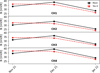 |
Fig. 9 Evolution with time of the on-sky responsivity (ℜ) calculated on Moon (black) and Tau A (red) observations. The results obtained on the four channels (CH) of TGI Pixel 23 are represented from top to bottom. |
5.3 Polarization angle
Table 10 summarizes the results of the polarization angle characterization with the three different setups. Section 3.5 details the results for ground characterization, Sect. 4.1.3 with Tau A, and Section 4.2.4 with the Moon. We notice a deviation of up to ~3 deg in a three-month variability. Finally, we expect a variation in the polarization angle across the bandwidth. Tau A, indeed, presents a synchrotron spectrum. At the same time, the diode may exhibit slight deviations from a perfect flat spectrum, primarily due to the directivity of the antenna to which it is coupled. The results from the different setups are compatible at ~3σ. Tau A provides the most reliable reference for the polarization angle because its emission is stable, well-characterized, and free from the geometric modeling uncertainties associated with lunar scattering. Therefore, the Tau A–based measurement offers the clearest on-sky calibration and ensures better control of systematics compared to the Moon.
Pixel 23 characterization comparison.
6 Conclusions
This work has presented the characterization of the TFGI experiment’s polarization efficiency, responsivity, and polarization angle, focusing on the central detector of the TFGI, Pixel 23. We began with ground-based diode reference measurements to quantify polarization efficiency, responsivity, and polarization angle. Additionally, we analyzed a dedicated dataset in which a rotating polarizer introduces multiple polarization angles to break degeneracies in the determination of instrumental angles. This dataset enables precise estimation of the detector’s polarization angle. We further used it to identify any systematic error angle associated with the phase switches relative to their expected configuration. Our results show that, within uncertainties, these error angles are consistent with 0 deg at the 2σ level and smaller than ~2 deg. Therefore, no additional correction is required for scientific exploitation of the data, ensuring polarization angle accuracy at the 1-deg level.
We extended our analysis using on-sky observations of Tau A and the Moon to further assess polarization efficiency, responsivity calibration, long-term responsivity stability, and the polarization angle. We observed responsivity variations by up to a factor of ~1.5 over a three-month period. Nevertheless, interchannel responsivity ratios remain stable within each dataset, suggesting that a common system component may be driving these changes.
In particular, the Moon observations provide an independent check on the instrumental polarization calibration. By assuming a fixed polarization efficiency from Tau A, we estimated the effective refraction index of the Moon at 31 GHz to be nMoon = 1.209 ± 0.007 (stat) ± 0.009 (sys), consistent with limb-weighted emission dominated by the uppermost surface layer and the previous measurement. This result aligns with previous findings that the apparent dielectric constant can vary significantly with surface roughness, reinforcing the Moon’s utility as a polarization calibrator at microwave frequencies.
This work highlights the need to implement a real-time system to monitor responsivity in conjunction with calibrator observations. This conclusion is motivated by the observed temporal variability of calibration parameters during commissioning, which demonstrates that continuous monitoring would be necessary to track and correct such effects in real time. Following the example of the MFI, we will install an internal diode calibrator to sample responsivity every 30 seconds. This system will provide a relative responsivity calibration for tracking stability, while absolute calibration will continue to rely on astrophysical sources, such as Tau A. The new diode system will enhance the mitigation of systematics and thus yield a more robust polarization angle determination and improved temporal stability of the instrument’s response.
The scientific goal is to achieve an absolute calibration performance for TFGI comparable to that obtained with the QUIJOTE MFI 11 GHz band (Rubiño-Martín et al. 2023), namely, an internal calibration uncertainty of ~1% and an overall uncertainty of ~5% when including systematic errors associated with the modeling of the calibrators. For the polarization angle, we aim for an accuracy of about 1 deg, similar to what is achieved at 11 GHz with MFI. In this work, the absolute responsivity (derived independently from Tau A and from the Moon) is consistent at the few-percent level. However, no internal calibration diode is currently installed, and therefore, the absolute responsivity is not yet stabilized across different observing periods. The internal consistency of the responsivity calibration is presently limited to a level of less than 8% due to residual systematic effects identified during commissioning. Regarding the polarization angle, we obtained uncertainties at the ~1 deg level, which is well within the <3 deg requirement inferred from previous QUIJOTE analyses (López Caraballo 2013). These performances are adequate for the primary QUIJOTE science goals at these frequencies.
Finally, we note that the analyses presented here do not account for variations across the frequency band. Conducting a detailed characterization of the bandpass will be essential in future work, as unmodeled frequency dependence may bias the measured polarization angle and, consequently, the inferred angle errors.
Acknowledgements
Some of the results presented in this work are based on observations obtained with the QUIJOTE experiment (doi.org/10.26698/quijote-mfi-dr1). We thank the staff of the Teide Observatory for invaluable assistance in the commissioning and operation of QUIJOTE. The QUIJOTE experiment is being developed by the Instituto de Astrofísica de Canarias (IAC), the Instituto de Fisica de Cantabria (IFCA), and the Universities of Cantabria, Manchester and Cambridge. Partial financial support was provided by the Spanish Ministry of Science and Innovation under the projects AYA2007-68058-C03-01, AYA2007-68058-C03-02, AYA2010-21766-C03-01, AYA2010-21766-C03-02, AYA2014-60438-P, ESP2015-70646-C2-1-R, AYA2017-84185-P, ESP2017-83921-C2-1-R, PGC2018-101814-B-I00, PID2019-110610RB-C21, PID2020-120514GB-I00, IACA13-3E-2336, IACA15-BE-3707, EQC2018-004918-P, PID2023-150398NB-I00 and PID2023-151567NB-I00, the Severo Ochoa Programs SEV-2015-0548 and CEX2019-000920-S, the Maria de Maeztu Program MDM-2017-0765, and by the Consolider-Ingenio project CSD2010-00064 (EPI: Exploring the Physics of Inflation). We acknowledge support from the ACIISI, Consejeria de Economia, Conocimiento y Empleo del Gobierno de Canarias and the European Regional Development Fund (ERDF) under grant with reference ProID2020010108, and Red de Investigación RED2022-134715-T funded by MCIN/AEI/10.13039/501100011033. This project has received funding from the European Union’s Horizon 2020 research and innovation program under grant agreement number 687312 (RADIOFOREGROUNDS), and the Horizon Europe research and innovation program under GA 101135036 (RadioForegroundsPlus). This research made use of computing time available on the high-performance computing systems at the IAC. We thankfully acknowledge the technical expertise and assistance provided by the Spanish Supercomputing Network (Red Española de Supercomputación), as well as the computer resources used: the Deimos/Diva Supercomputer, located at the IAC. This research used resources of the National Energy Research Scientific Computing Center, that is supported by the Office of Science of the U.S. Department of Energy under Contract No. DE-AC02-05CH11231. MFT acknowledges support from the Enigmass+ research federation (CNRS, Université Grenoble Alpes, Université Savoie Mont-Blanc). Some of the results in this work have been derived using the healpy and HEALPix packages (Górski et al. 2005; Zonca et al. 2019). We have also used scipy (Virtanen et al. 2020), emcee (Foreman-Mackey et al. 2013), numpy (Harris et al. 2020), matplotlib (Hunter 2007), corner (Foreman-Mackey 2016) and astropy (Astropy Collaboration et al. 2013; Astropy Collaboration 2018) PYTHON packages.
References
- Abazajian, K. N., Adshead, P., Ahmed, Z., et al. 2016, arXiv e-prints [arXiv:1610.02743] [Google Scholar]
- Abitbol, M. H., Alonso, D., Simon, S. M., et al. 2021, JCAP, 2021, 032 [CrossRef] [Google Scholar]
- Adachi, S., Adkins, T., Aguilar Faúndez, M. A. O., et al. 2022, ApJ, 931, 101 [CrossRef] [Google Scholar]
- Ade, P., Aguirre, J., Ahmed, Z., et al. 2019, JCAP, 2019, 056 [Google Scholar]
- Ade, P. A. R., Amiri, M., Benton, S. J., et al. 2022, ApJ, 927, 174 [CrossRef] [Google Scholar]
- Artal, E., Aja, B., de la Fuente, L., Hoyland, R., & Villa, E. 2020, SPIE Conf. Ser., 11453, 1145316 [Google Scholar]
- Astropy Collaboration (Robitaille, T. P., et al.) 2013, A&A, 558, A33 [NASA ADS] [CrossRef] [EDP Sciences] [Google Scholar]
- Astropy Collaboration (Price-Whelan, A. M., et al.) 2018, AJ, 156, 123 [Google Scholar]
- Aumont, J., Macías-Pérez, J. F., Ritacco, A., et al. 2020, A&A, 634, A100 [CrossRef] [EDP Sciences] [Google Scholar]
- Bennett, C. L., Larson, D., Weiland, J. L., et al. 2013, ApJS, 208, 20 [Google Scholar]
- Betoule, M., Pierpaoli, E., Delabrouille, J., Le Jeune, M., & Cardoso, J. F. 2009, A&A, 503, 691 [NASA ADS] [CrossRef] [EDP Sciences] [Google Scholar]
- BICEP/Keck Collaboration (Ade, P. A. R., et al.) 2022, ApJ, 927, 77 [NASA ADS] [CrossRef] [Google Scholar]
- Bischoff, C. 2010, PhD thesis, University of Chicago, USA [Google Scholar]
- Born, M., & Wolf, E. 1959, Principles of Optics Electromagnetic Theory of Propagation, Interference and Diffraction of Light [Google Scholar]
- Calla, O. P. N., & Rathore, I. S. 2012, Adv. Space Res., 50, 1607 [Google Scholar]
- Carralot, F., Carones, A., Krachmalnicoff, N., et al. 2025, JCAP, 2025, 019 [Google Scholar]
- Casas, F. J., Martínez-González, E., Bermejo-Ballesteros, J., et al. 2021, Sensors, 21, 3361 [Google Scholar]
- Chown, R., Omori, Y., Aylor, K., et al. 2018, ApJS, 239, 10 [Google Scholar]
- Coppi, G., Astori, F., Rancati Cattaneo, G., et al. 2024, SPIE Conf. Ser., 13102, 1310224 [Google Scholar]
- Dahal, S., Brewer, M. K., Akins, A. B., et al. 2023, Planet. Sci. J., 4, 154 [Google Scholar]
- Eimer, J. R., Li, Y., Brewer, M. K., et al. 2024, ApJ, 963, 92 [NASA ADS] [CrossRef] [Google Scholar]
- Essinger-Hileman, T., Ali, A., Amiri, M., et al. 2014, SPIE Conf. Ser., 9153, 91531I [Google Scholar]
- Fernández-Torreiro, M. 2023, PhD thesis, Universidad de La Laguna [Google Scholar]
- Foreman-Mackey, D. 2016, J. Open Source Softw., 1, 24 [Google Scholar]
- Foreman-Mackey, D., Hogg, D. W., Lang, D., Goodman, & Jonathan. 2013, PASP, 125, 306 [CrossRef] [Google Scholar]
- Gómez-Reñasco, M. F., Martín, Y., Aguiar-González, M., et al. 2016, Proc. SPIE, 9914, 991432 [Google Scholar]
- Górski, K. M., Hivon, E., Banday, A. J., et al. 2005, ApJ, 622, 759 [Google Scholar]
- Hafez, Y. A., Trojan, L., Albaqami, F. H., et al. 2014, MNRAS, 439, 2271 [Google Scholar]
- Harris, C. R., Millman, K. J., van der Walt, S. J., et al. 2020, Nature, 585, 357 [NASA ADS] [CrossRef] [Google Scholar]
- Hazumi, M., Ade, P. A. R., Akiba, Y., et al. 2019, J. Low Temp. Phys., 194, 443 [Google Scholar]
- Hinshaw, G., Larson, D., Komatsu, E., et al. 2013, ApJS, 208, 19 [Google Scholar]
- Hoyland, R., Aguiar-González, M., Génova-Santos, R., et al. 2014, SPIE Conf. Ser., 9153, 915332 [Google Scholar]
- Hui, H., Ade, P. A. R., Ahmed, Z., et al. 2018, SPIE Conf. Ser., 10708, 1070807 [Google Scholar]
- Hunter, J. D. 2007, Comput. Sci. Eng., 9, 90 [NASA ADS] [CrossRef] [Google Scholar]
- Inoue, Y., Ade, P., Akiba, Y., et al. 2016, SPIE Conf. Ser., 9914, 99141I [Google Scholar]
- Kamionkowski, M., Kosowsky, A., & Stebbins, A. 1997, Phys. Rev. D, 55, 7368 [NASA ADS] [CrossRef] [Google Scholar]
- Keihm, S. J. 1984, Icarus, 60, 568 [Google Scholar]
- Kogut, A., Banday, A. J., Bennett, C. L., et al. 1996, ApJ, 460, 1 [NASA ADS] [CrossRef] [Google Scholar]
- Kusaka, A., Appel, J., Essinger-Hileman, T., et al. 2018, JCAP, 2018, 005 [Google Scholar]
- Li, Y., Austermann, J. E., Beall, J. A., et al. 2021, IEEE Trans. Appl. Supercond., 31, 3063334 [Google Scholar]
- LiteBIRD Collaboration, Allys, E., Arnold, K., et al. 2023, Progr. Theor. Exp. Phys., 2023, 042F01 [CrossRef] [Google Scholar]
- López Caraballo, C. H. 2013, PhD thesis, University of La Laguna, Spain [Google Scholar]
- Losovskii, B. Y. 1967, Soviet Ast., 11, 329 [Google Scholar]
- Mennella, A., Ade, P., Almela, A., et al. 2024, in European Physical Journal Web of Conferences, 293, mm Universe 2023 – Observing the Universe at mm Wavelengths, 00030 [Google Scholar]
- Murata, M., Nakata, H., Iijima, K., et al. 2023, Rev. Sci. Instrum., 94, 124502 [Google Scholar]
- O’Dea, D., Challinor, A., & Johnson, B. R. 2007, MNRAS, 376, 1767 [CrossRef] [Google Scholar]
- Olhoeft, G. R., & Strangway, D. W. 1975, Earth Planet. Sci. Lett., 24, 394 [CrossRef] [Google Scholar]
- Olhoeft, G. R., Strangway, D. W., & Frisillo, A. L. 1973, Lunar Planet. Sci. Conf. Proc., 4, 3133 [Google Scholar]
- Pérez-de-Taoro, M. R., Aguiar-González, M., Cózar-Castellano, J., et al. 2016, Proc. SPIE, 9906, 99061K [Google Scholar]
- Perley, R. A., & Butler, B. J. 2013, ApJSS, 206, 16 [NASA ADS] [CrossRef] [Google Scholar]
- Planck Collaboration IV. 2016, A&A, 594, A4 [NASA ADS] [CrossRef] [EDP Sciences] [Google Scholar]
- Planck Collaboration VI. 2016, A&A, 594, A6 [NASA ADS] [CrossRef] [EDP Sciences] [Google Scholar]
- Planck Collaboration VI. 2020, A&A, 641, A6 [NASA ADS] [CrossRef] [EDP Sciences] [Google Scholar]
- Qu, F. J., Sherwin, B. D., Madhavacheril, M. S., et al. 2024, ApJ, 962, 112 [NASA ADS] [CrossRef] [Google Scholar]
- Ritacco, A., Macías-Pérez, J. F., Ponthieu, N., et al. 2018, A&A, 616, A35 [NASA ADS] [CrossRef] [EDP Sciences] [Google Scholar]
- Ritacco, A., Bizzarri, L., Boulanger, F., et al. 2024, in European Physical Journal Web of Conferences, 293, 00044 [Google Scholar]
- Rubiño-Martín, J. A., Génova-Santos, R., Rebolo, R., et al. 2017, in Highlights on Spanish Astrophysics IX, eds. S. Arribas, A. Alonso-Herrero, F. Figueras, C. Hernández-Monteagudo, A. Sánchez-Lavega, & S. Pérez-Hoyos, 99 [Google Scholar]
- Rubiño-Martín, J. A., Génova-Santos, R., Rebolo, R., et al. 2017, in Highlights on Spanish Astrophysics IX, eds. S. Arribas, A. Alonso-Herrero, F. Figueras, C. Hernández-Monteagudo, A. Sánchez-Lavega, & S. Pérez-Hoyos, 99 [Google Scholar]
- Rubiño-Martín, J. A., Guidi, F., Génova-Santos, R. T., et al. 2023, MNRAS, 519, 3383 [NASA ADS] [CrossRef] [Google Scholar]
- Sánchez-de-la-Rosa, V., Vega-Moreno, A., Cózar-Castellano, J., et al. 2016, Proc. SPIE, 9914, 99142N [Google Scholar]
- Seljak, U., & Zaldarriaga, M. 1997, Phys. Rev. Lett., 78, 2054 [Google Scholar]
- Shaw, E. C., Ade, P. A. R., Akers, S., et al. 2024, SPIE Conf. Ser., 13102, 1310204 [Google Scholar]
- Simon, S. M., Appel, J. W., Campusano, L. E., et al. 2016, J. Low Temp. Phys., 184, 534 [Google Scholar]
- Sobrin, J. A., Anderson, A. J., Bender, A. N., et al. 2022, ApJS, 258, 42 [NASA ADS] [CrossRef] [Google Scholar]
- Stebor, N., Ade, P., Akiba, Y., et al. 2016, SPIE Conf. Ser., 9914, 99141H [Google Scholar]
- Strangway, D. W., Pearce, G. W., & Olhoeft, G. R. 1977, in NASA Special Publication, 370, eds. J. H. Pomeroy & N. J. Hubbard, 417 [Google Scholar]
- Tinbergen, J. 1996, Astronomical Polarimetry (Cambridge University Press) [Google Scholar]
- Tristram, M., Banday, A. J., Górski, K. M., et al. 2022, Phys. Rev. D, 105, 083524 [Google Scholar]
- Tsujii, M., Baselmans, J. J. A., Choi, J., et al. 2024, SPIE Conf. Ser., 13102, 1310205 [Google Scholar]
- Vielva, P., Martínez-González, E., Casas, F. J., et al. 2022, JCAP, 2022, 029 [CrossRef] [Google Scholar]
- Virtanen, P., Gommers, R., Oliphant, T. E., et al. 2020, Nat. Methods, 17, 261 [Google Scholar]
- Wang, Z., Li, Y., Jiang, J., & Li, D. 2010, Sci. China Earth Sci., 53, 1365 [Google Scholar]
- Weiland, J. L., Odegard, N., Hill, R. S., et al. 2011, ApJS, 192, 19 [Google Scholar]
- Xu, Z., Brewer, M. K., Fluxá Rojas, P., et al. 2020, ApJ, 891, 134 [Google Scholar]
- Xu, Z., Brewer, M. K., Rojas, P. F., et al. 2020, ApJ, 891, 134 [Google Scholar]
- Zheng, Y. C., Tsang, K. T., Chan, K. L., et al. 2012, Icarus, 219, 194 [CrossRef] [Google Scholar]
- Zonca, A., Singer, L., Lenz, D., et al. 2019, J. Open Source Softw., 4, 1298 [Google Scholar]
Not to be mistaken this time with the Stokes V parameter.
The polarization loss is defined as: 100% − η.
gI is considered a single parameter to simplify the system, rather than fitting g and I separately.
This translates into a decrease of the flux density by a factor ![Mathematical equation: $\[\exp \left[\frac{-0.21}{100}(2021.9-2016.3)\right]=0.9883\]$](/articles/aa/full_html/2026/04/aa58376-25/aa58376-25-eq34.png) .
.
We considered only the nominal frequencies of TFGI, 31 and 41 GHz. Color corrections were simulated assuming a top-hat band and were found to be negligible (<1%), so they were not applied.
Appendix A Effective refraction index of the Moon at 31 GHz under a smooth-surface assumption
We estimate the effective refraction index of the Moon (nMoon) at 31 GHz by exploiting its role as a polarization calibrator. Direct estimates of polarization efficiency from Moon observations present large uncertainties. To address this issue, we fix the polarization efficiency for each channel to the values derived from Tau A measurements (see Table 4), which align with independent ground-based calibrations (see the top of Table 1), and solve for the value of nMoon that minimizes the residuals between the observed and simulated Moon polarization maps. The resulting estimates of the Moon’s refraction index are summarized in Table A.1.
From this procedure, we derive an effective refraction index of nMoon = 1.209 ± 0.007 (stat) ± 0.009 (sys) To estimate the systematic uncertainty, we first reran the calculation varying the beam FWHM by 2%, based on the TGI beam ellipticity analysis (see Fernández-Torreiro 2023), obtaining a contribution of 0.005. In addition, we considered potential intensity-to-polarization leakage. Assuming a conservative worst-case scenario of 0.5% leakage from intensity into both Q and U, as expected during high-speed telescope scanning (Fernández-Torreiro 2023), this effect contributes an additional 0.008 to the refraction index. These two contributions are combined in quadrature, yielding the quoted systematic uncertainty of 0.009. Additional factors, such as the assumed polarization model, viewing geometry, surface heterogeneity, and limb dominance, which are not included in this analysis, may also contribute to systematic uncertainties. The quoted systematic uncertainty should therefore be regarded as a lower limit.
Interestingly, our estimated nMoon aligns closely with the value of nMoon ~ 1.25 independently derived by Génova-Santos et al. (in prep.) using observations of Tau A obtained with the Sardinia Radio Telescope (SRT). This consistency indicates a potential trend toward lower effective refraction indices when probing the Moon’s surface through polarization-sensitive measurements, particularly at microwave frequencies.
An earlier estimate by Losovskii (1967) reported a dielectric constant of ϵMoon = 1.5 ± 0.2 at ~38 GHz, corresponding to ![Mathematical equation: $\[n_{\text {Moon }}=\sqrt{\epsilon_{\text {Moon }}}=1.22 \pm 0.08\]$](/articles/aa/full_html/2026/04/aa58376-25/aa58376-25-eq25.png) , based on a smooth, isotropic, non-magnetic lunar surface model. This result is compatible with ours within 1σ. Notably, the author emphasized that including diffuse scattering from small-scale surface roughness results in a higher effective dielectric constant.
, based on a smooth, isotropic, non-magnetic lunar surface model. This result is compatible with ours within 1σ. Notably, the author emphasized that including diffuse scattering from small-scale surface roughness results in a higher effective dielectric constant.
More recent studies generally report higher refraction indices, typically in the range nMoon ~ 1.5–1.9, based on laboratory measurements of Apollo regolith samples (e.g., Olhoeft et al. 1973; Olhoeft & Strangway 1975; Calla & Rathore 2012), detailed electromagnetic modeling (e.g., Strangway et al. 1977; Keihm 1984), and orbital observations from microwave radiometers aboard missions such as Chang’E-1/2 (see Zheng et al. 2012). These works typically incorporate more complete dielectric models and consider the bulk properties of compacted regolith.
In contrast, our measurement is derived from polarized emission near the lunar limb. Consequently, our analysis probes the uppermost surface layer – a porous, low-density region that is not well represented by the bulk permittivity of the deeper regolith. This interpretation is supported by spatial variations observed in microwave emissivity and dielectric constant maps (e.g., Wang et al. 2010).
Effective refraction index of the Moon at 31 GHz (nMoon).
Appendix B Data visualization and structure
In this Appendix, we clarify the data structure by visualizing the output data for each phase state and channel, segmented by the single polarizer angle within the shaded region. Figure B.1 presents the results.
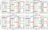 |
Fig. B.1 Data displayed for each phase state. From left to right and from top to bottom: 0, 90, 180, and 270 deg. Within each subplot, the output for the four channels is shown. The polarizer angle change is represented by alternating white and gray shades within each subplot. |
Appendix C Stokes parameters equations and polarization efficiency
We list all the equations for the Q and U Stokes parameters for each channel combination:
![Mathematical equation: $\[-Q_{\mathrm{TGI}, \mathrm{FGI}}=V_{1,4}(90 ~\mathrm{deg})-V_{1,4}(270 ~\mathrm{deg}),\]$](/articles/aa/full_html/2026/04/aa58376-25/aa58376-25-eq26.png) (C.1)
(C.1)
![Mathematical equation: $\[+U_{\mathrm{TGI}, \mathrm{FGI}}=V_{1,4}(0 ~\mathrm{deg})-V_{1,4}(180 ~\mathrm{deg}),\]$](/articles/aa/full_html/2026/04/aa58376-25/aa58376-25-eq27.png) (C.2)
(C.2)
![Mathematical equation: $\[+Q_{\mathrm{TGI}, \mathrm{FGI}}=V_{2,3}(90 ~\mathrm{deg})-V_{2,3}(270 ~\mathrm{deg}),\]$](/articles/aa/full_html/2026/04/aa58376-25/aa58376-25-eq28.png) (C.3)
(C.3)
![Mathematical equation: $\[-U_{\mathrm{TGI}, \mathrm{FGI}}=V_{2,3}(0 \operatorname{deg})-V_{2,3}(180 \operatorname{deg}),\]$](/articles/aa/full_html/2026/04/aa58376-25/aa58376-25-eq29.png) (C.4)
(C.4)
![Mathematical equation: $\[+Q_{\mathrm{TGI}, \mathrm{FGI}}=V_{3,1}(0 ~\mathrm{deg})-V_{3,1}(180 ~\mathrm{deg}),\]$](/articles/aa/full_html/2026/04/aa58376-25/aa58376-25-eq30.png) (C.5)
(C.5)
![Mathematical equation: $\[+U_{\mathrm{TGI}, \mathrm{FGI}}=V_{3,1}(90 ~\mathrm{deg})-V_{3,1}(270 ~\mathrm{deg}),\]$](/articles/aa/full_html/2026/04/aa58376-25/aa58376-25-eq31.png) (C.6)
(C.6)
![Mathematical equation: $\[-Q_{\mathrm{TGI}, \mathrm{FGI}}=V_{4,2}(0 ~\mathrm{deg})-V_{4,2}(180 ~\mathrm{deg}),\]$](/articles/aa/full_html/2026/04/aa58376-25/aa58376-25-eq32.png) (C.7)
(C.7)
![Mathematical equation: $\[-U_{\mathrm{TGI}, \mathrm{FGI}}=V_{4,2}(90 ~\mathrm{deg})-V_{4,2}(270 ~\mathrm{deg}).\]$](/articles/aa/full_html/2026/04/aa58376-25/aa58376-25-eq33.png) (C.8)
(C.8)
The subscript refers to the TGI and FGI channels, respectively. Table C.1 shows the results of the polarization efficiency for each channel and polarizer angle. The missing data occurs when the polarization efficiency exceeds 100% due to a spike in the first dataset at 45 deg in the polarizer angle. Overall, the polarization efficiency remains well above the 90% value, confirming a polarization loss across all combinations. The first columns present the results for the three datasets described in Sect. 3.2, while the last column summarizes the results by displaying the mean value (Mean CH) and standard deviation (STD) for each channel and polarizer angle across datasets.
Polarization efficiency (η) for each channel and polarizer angle.
Appendix D Polarization angle with diode reference
Table D.1 presents the value of the polarization angle for each channel and polarizer angle. The study details are provided in Sect. 3.5. The study was conducted with the datasets 2022_April_06_1, 2022_April_06_2, and 2022_April_07_3 described in Sect. 3.2.
Polarization angle for each channel and polarizer angle.
Appendix E Phase error fitting visualization and comparison with the data
This section presents the visual results of the fitting function applied to the actual data in Fig. E.1,E.2,E.3. For the datasets 2022_April_06_1, 2022_April_06_2, and 2022_April_07_3 described in Sect. 3.2.
Including the ϵ parameters in the fitting does not significantly affect the quality of the results regarding residuals, based on an equivalent 0-deg angle correction. We observe inconsistencies in the fitting process as we approach the 0-V signal. This effect arises because the polarization efficiency does not reach 100% (as reported in Appendix C). The results of these fittings are displayed in Figure E.4.
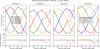 |
Fig. E.1 Visual representation of the fitting process for dataset Pixel23_2022_April_06_1. The recorded data are shown with continuous lines, while the fitting model incorporating γref is illustrated with dashed lines, and the model integrating ϵ is displayed with dotted lines. We do not use this dataset for calculating ϵ due to the presence of spikes. |
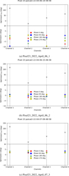 |
Fig. E.4 Average error angle correction, ϵ, in the three datasets along with their standard deviations for each channel. The average γref reported here (< γref >) has to be corrected to obtain the on-sky polarization angle, ϕc (see Eq. (6)). The first dataset is not valid for the ϵ calculation due to the occurrence of a spike in the polarizer angle at 45 deg. |
All Tables
All Figures
|
Fig. 1 Block diagrams of the receivers (one detector). Top: 30-GHz Instrument. Bottom: 40-GHz Instrument. The diagram is taken from Artal et al. (2020). |
| In the text | |
|
Fig. 2 Photo of the MFCI mounted on the calibration alignment plate. The diode used introduces the known signal into the TFGI detectors. The fixed plate is placed on top of the focal plane and defines the different detector locations where the diode can be positioned. The rotary motor allows for the modification of the calibration diode’s orientation (γ) in 22.5 deg steps to study different linear polarization inputs. A detailed description is presented in Fernández-Torreiro (2023). |
| In the text | |
|
Fig. 3 Example of a full data block, ~8 ms. The left part of the voltage output shows the diode “ON”, while the right part shows the diode “OFF”. Each color identifies a channel output. The signal exhibits saturation, reaching a value of 10 V, in some cases. |
| In the text | |
|
Fig. 4 Histogram of the slopes that quantify the signal stability in a data acquisition of 1 minute. Each count is defined as a function of the slope obtained from linear fitting. The slope values span a range of ~ −2.5–0.5 mV/min for the diode ON case, indicating a lack of significant stability issues within 1 minute of integration. |
| In the text | |
|
Fig. 5 Schematic of the polarization angle measurement of the telescope. The axes represent the ground tilt (Horizontal) and the deviation from zenith (Vertical). |
| In the text | |
|
Fig. 6 Maps of the single Tau A observation used to estimate polarization efficiency, smoothed at 1 deg. We discuss in Sect. 4.1.3 how these uncalibrated maps are utilized to calculate the polarization angle. From top to bottom, the rows show the Stokes parameters I, Q, U, and polarized intensity P. From left to right, the columns show channels 1, 2, 3, and 4. |
| In the text | |
|
Fig. 7 Schematic describing the Moon’s emission model and the parameters involved: the refraction index of the Moon (nMoon), the refraction index of free space (nt), the incident (θi) and transmitted (θt) angles, the radial coordinate (r′), and the radius of the Moon (R). |
| In the text | |
|
Fig. 8 Moon maps of the three Stokes parameters I, Q, and U and of the polarized intensity P for an observation taken on December 2021 (left) and for the simulated model inferred from the observation parameters (right). |
| In the text | |
|
Fig. 9 Evolution with time of the on-sky responsivity (ℜ) calculated on Moon (black) and Tau A (red) observations. The results obtained on the four channels (CH) of TGI Pixel 23 are represented from top to bottom. |
| In the text | |
|
Fig. B.1 Data displayed for each phase state. From left to right and from top to bottom: 0, 90, 180, and 270 deg. Within each subplot, the output for the four channels is shown. The polarizer angle change is represented by alternating white and gray shades within each subplot. |
| In the text | |
|
Fig. E.1 Visual representation of the fitting process for dataset Pixel23_2022_April_06_1. The recorded data are shown with continuous lines, while the fitting model incorporating γref is illustrated with dashed lines, and the model integrating ϵ is displayed with dotted lines. We do not use this dataset for calculating ϵ due to the presence of spikes. |
| In the text | |
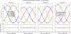 |
Fig. E.2 Same as Fig. E.1 but for dataset Pixel23_2022_April_06_2. |
| In the text | |
 |
Fig. E.3 Same as Fig. E.1 and Fig. E.2 but for dataset Pixel23_2022_April_07_3. |
| In the text | |
|
Fig. E.4 Average error angle correction, ϵ, in the three datasets along with their standard deviations for each channel. The average γref reported here (< γref >) has to be corrected to obtain the on-sky polarization angle, ϕc (see Eq. (6)). The first dataset is not valid for the ϵ calculation due to the occurrence of a spike in the polarizer angle at 45 deg. |
| In the text | |
Current usage metrics show cumulative count of Article Views (full-text article views including HTML views, PDF and ePub downloads, according to the available data) and Abstracts Views on Vision4Press platform.
Data correspond to usage on the plateform after 2015. The current usage metrics is available 48-96 hours after online publication and is updated daily on week days.
Initial download of the metrics may take a while.