| Issue |
A&A
Volume 708, April 2026
|
|
|---|---|---|
| Article Number | A212 | |
| Number of page(s) | 19 | |
| Section | Extragalactic astronomy | |
| DOI | https://doi.org/10.1051/0004-6361/202558420 | |
| Published online | 08 April 2026 | |
MEDUSA
I. Tracing magnetic field structures in tidal arms of the dwarf–dwarf merger NGC 1487
1
Ruhr University Bochum, Faculty of Physics and Astronomy, Astronomical Institute (AIRUB), Universitätsstraße 150, 44801 Bochum, Germany
2
Ruhr Astroparticle and Plasma Physics Center (RAPP Center), 44780 Bochum, Germany
3
CSIRO Space and Astronomy, PO Box 1130 Bentley, WA 6102, Australia
4
Thüringer Landessternwarte, Sternwarte 5, 07778 Tautenburg, Germany
5
Max-Planck-Institut für Radioastronomie, Auf dem Hügel 69, 53121 Bonn, Germany
6
Ruhr University Bochum, Faculty for Physics & Astronomy, Theoretical Physics IV: Plasma Astroparticle Physics, 44780 Bochum, Germany
7
SKA Observatory, SKA-Low Science Operations Centre, 26 Dick Perry Avenue, Kensington, WA 6151, Australia
8
INAF – Osservatorio Astronomico di Cagliari, Via della Scienza 5, Selargius, Italy
9
Astronomical Observatory of the Jagiellonian University, ul. Orla 171, 30-244 Kraków, Poland
10
Department of Space, Earth and Environment, Chalmers University of Technology, Gothenburg, Sweden
★ Corresponding author: This email address is being protected from spambots. You need JavaScript enabled to view it.
Received:
5
December
2025
Accepted:
21
February
2026
Abstract
Context. Radio continuum observations of dwarf–dwarf galaxy mergers, such as NGC 1487, provide crucial insights into magnetic field amplification and cosmic ray (CR) propagation during galactic assembly. Dwarf galaxies are important laboratories for studying cosmic magnetism because they can maintain strong magnetic fields via the action of turbulent dynamo despite their low mass and weak gravitational potential.
Aims. The Magnetic-field Evolution in Dwarf galaxies from Ultra-deep SKA Analysis (MEDUSA) survey is the first SKA-pathfinder programme designed to obtain deep continuum, polarisation, and H I data for dwarf galaxies, enabling a comprehensive study of their radio spectra, magnetic fields, and gas kinematics across a representative population. By analysing the radio continuum spectra and polarisation of the dwarf–dwarf galaxy merger NGC 1487 from the MEDUSA sample, our aim was to determine its magnetic field strength and to characterise the large-scale and turbulent components of its magnetic field.
Methods. We utilised highly sensitive multi-band radio continuum data from MeerKAT L-band (1.28 GHz) and Australia Telescope Compact Array (ATCA) L/S (2.1 GHz), C (5.5 GHz), and X-bands (9 GHz). We analysed the magnetic field configuration using polarisation and rotation measure (RM) synthesis.
Results. The integrated spectral energy distribution has a non-thermal spectral index of αnth = −0.678 ± 0.085, indicating a significant synchrotron contribution, consistent with a CR electron injection index of γ = 2.36 (N(E)∝E−γ) typical of supernova remnants. Synchrotron and inverse Compton losses cause a spectral break at νb = 6.2 ± 1.3 GHz. In star-forming regions, the magnetic field exhibits strong small-scale fluctuations in RM, suggesting the action of a small-scale dynamo. Conversely, the field becomes more ordered, aligning with the tidal arms towards the galaxy’s outskirts, showing a large-scale magnetic field over ≈3 kpc. The CR cooling timescale of approximately 11 Myr at 1.28 GHz is similar to the escape timescale.
Conclusions. Observations of the dwarf–dwarf merger NGC 1487 show that even low-mass galaxy mergers, likely the building blocks of larger galaxies in the early Universe, can rapidly amplify and produce coherent large-scale magnetic field structures, highlighting their contribution in the early magnetisation of galaxies.
Key words: cosmic rays / ISM: magnetic fields / ISM: structure / Galaxy: evolution / galaxies: dwarf / galaxies: individual: NGC 1487
© The Authors 2026
 Open Access article, published by EDP Sciences, under the terms of the Creative Commons Attribution License (https://creativecommons.org/licenses/by/4.0), which permits unrestricted use, distribution, and reproduction in any medium, provided the original work is properly cited.
This article is published in open access under the Subscribe to Open model. This email address is being protected from spambots. You need JavaScript enabled to view it. to support open access publication.
1. Introduction
Galaxy mergers are a fundamental process in the Universe; they shape the evolution of galaxies by driving mass assembly, altering morphology, and influencing star formation rates (Mićić et al. 2022; Papaderos et al. 2012; Henkel et al. 2022). Among these processes, mergers between dwarf galaxies are particularly significant, as dwarf galaxies are the most common type (e.g. Henkel et al. 2022) and serve as essential building blocks for larger systems. Their low mass and weak gravitational potential make them strongly subject to external influences such as tidal interactions, and to the effects of stellar feedback (Buzzo et al. 2021; Kronberg 2016; Mengel et al. 2008). Compared to more massive galaxies, these dwarf galaxies rotate more slowly, reducing the efficiency of the Ω-dynamo and hence the amplification of large-scale magnetic fields (e.g. Beck & Wielebinski 2013). At the same time, their shallow gravitational potential allows stellar feedback to launch stronger outflows (Buzzo et al. 2021). Even though their slow rotation and shallow gravitational wells would typically limit large-scale dynamo action, dwarf galaxies can still sustain strong magnetic fields powered by intense star formation and supernova-driven turbulence (e.g. Chyży et al. 2016; Kepley et al. 2010; Basu et al. 2017b; Kepley et al. 2011). This makes them key systems for investigating the fast magnetic field amplification processes believed to shape magnetic fields in the early Universe (Schleicher & Beck 2013; Kronberg 2016; Rodenbeck & Schleicher 2016). Simulations show that magnetic field strength in galaxy mergers exhibits two peaks: the first during initial core approach and the second just before coalescence, driven by tidal forces and angular momentum transport (Rodenbeck & Schleicher 2016). In the central regions, fields are amplified by angular momentum transport, while in the outer regions, geometric projection effects enhance observed strength. Additionally, shear forces and Kelvin-Helmholtz instabilities in outflows further amplify magnetic fields (Kronberg 2016).
Radio continuum observations provide crucial information into galactic magnetic fields, including their strength (Beck et al. 2019) and orientation via polarisation (Brentjens & de Bruyn 2005; Pakmor et al. 2018; Reissl et al. 2023). Additionally, they serve as a powerful tool for studying cosmic ray (CR) transport and energy loss mechanisms (synchrotron, inverse-Compton, and bremsstrahlung) using synchrotron emission as tracers (e.g. Lacki et al. 2010; Werhahn et al. 2021; Pfrommer et al. 2022; Heesen et al. 2022. CRs produced in supernova remnants travel into the halo through advection, diffusion, and streaming (e.g. Strong et al. 2007; Stein et al. 2019; Thomas et al. 2020), exciting Alfvén and whistler waves that scatter them and regulate their drift speed (Kulsrud & Pearce 1969; Shalaby et al. 2021, 2023; Lemmerz et al. 2025). This coupling allows CRs to transfer momentum to the gas and generate pressure support that can drive large-scale galactic winds, a key feature of CR hydrodynamic models (Zweibel 2013; Pfrommer et al. 2017a; Thomas & Pfrommer 2019). Magneto-hydrodynamic simulations have shown that such CR-driven winds can significantly influence mass loading, halo gas distribution, and star formation (e.g. Breitschwerdt et al. 1991; Uhlig et al. 2012; Pakmor et al. 2016; Girichidis et al. 2016; Recchia et al. 2017; Dashyan & Dubois 2020; Thomas et al. 2023). This study extends earlier radio continuum (e.g. ChyŻy et al. 2000; Kepley et al. 2010; Chyży et al. 2016; Kepley et al. 2011; Basu et al. 2017b; Taziaux et al. 2025), by using low-frequency observations to trace CR electrons (CREs) into galaxy halos and to characterise their energy losses. CR protons dominate in dense gas through hadronic interactions (Pfrommer & Enßlin 2004a; Pfrommer et al. 2017b; Werhahn et al. 2023), while synchrotron-emitting CREs probe lower-density outflows (Ruszkowski & Pfrommer 2023). CRs can also advect magnetic fields into galaxy halos, an effect expected to be especially strong in dwarf galaxies with shallow gravitational potentials. However, detecting CR-driven winds in dwarfs is observationally difficult because their synchrotron halos are faint, low in surface brightness, and easily diluted by thermal emission (e.g. Heesen et al. 2018; Taziaux et al. 2025). Low-frequency observations, with their enhanced sensitivity to older CRE populations, are therefore particularly well suited to testing CR feedback and its influence on magnetic fields.
In this paper, we present a full Stokes continuum study of the dwarf–dwarf merger NGC 1487 to explore the outflow kinematics, magnetic field structure, the dependence of energy loss mechanisms and the CR transport in dwarf galaxy mergers. These datasets represent the most sensitive set of radio continuum observations of this low-mass merger NGC 1487 to date and the first observations of their radio continuum and polarised emission at 1.28, 2.1, 5.5, and 9 GHz. We describe our dataset and reduction in Sect. 2. Spectral properties are analysed in Sect. 3. In Sect. 4, we describe the magnetic field configuration based on polarisation measurement and Faraday rotation. Further, in Sect. 5, the scope of modelling the CR transport in the scenario of NGC 1487 is explored. We will discuss the role of the magnetic field and the CR transport in Sect. 6 and the work is summarised in Sect. 7. Throughout the paper, we use the Gaussian cgs unit system.
2. Observation and data reduction
2.1. Selection of target
The Magnetic-field Evolution in Dwarf galaxies from Ultra-deep SKA Analysis (MEDUSA) survey is a radio polarimetry program (PI: S. Taziaux) using the MeerKAT telescope to study magnetic fields, neutral hydrogen, and CR transport in low-mass galaxies. The survey targets a representative sample of 13 nearby dwarf galaxies (D ≲ 13 Mpc) covering a broad range of morphologies, gas fractions, star formation rates, and evolutionary stages. Systems include isolated dwarfs, and low-mass mergers, selected to enable resolved studies of synchrotron emission, depolarisation, and H I kinematics. The full sample selection and survey strategy are described in Taziaux (in prep.).
Within this study, NGC 1487 was selected for an in-depth case study because it is a gas-rich, pre-merger dwarf galaxy (Buzzo et al. 2021). In Fig. 1, we show the optical, Hα and far-ultraviolet (FUV) images overlaid with the MeerKAT L-band observations, revealing overlapping discs, tidal tails, and ongoing starbursts, characteristic of an early-stage merger (Buzzo et al. 2021; Bergvall & Johansson 1995). Its tidal arms host active star formation, with star cluster mass distributions following a power law and star formation rate densities of (0.345 ± 0.024)×10−3 M⊙ yr−1 kpc−2 (east arm) and (0.360 ± 0.024)×10−3 M⊙ yr−1 kpc−2 (west arm) (Rodruck et al. 2023). Kinematic and metallicity maps indicate gas inflows, metal mixing, and disk rebuilding in the northern tail (Buzzo et al. 2021). A summary of the basic properties is shown in Table 1.
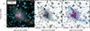 |
Fig. 1. Colour-composite images from the DESI Legacy Imaging Surveys (left panel), HIPASS Hα image (middle panel) and GALEX FUV image (right panel) of NGC 1487 with overlaid MeerKAT radio emission contours starting at 3 σI and increase by a factor of 2 at a central frequency of 1.28 GHz (σI = 4 μJy/beam). The beam of 8.56″ × 7.65″ is shown in the left corner. The scale is calculated using the distance given in Table 1. |
Summary of the basic properties of NGC 1487.
NGC 1487 provides an ideal case to address key MEDUSA science goals. Its highly disturbed gas kinematics and ongoing starburst activity (Buzzo et al. 2021) create conditions to study magnetic-field structure under strong turbulence and to characterise the spectral behavior of the radio continuum, including energy losses of CREs and free–free absorption in dense star-forming regions. Combined with deep MeerKAT continuum and broadband data, comparing to existing optical, UV, and MUSE observations, this dataset enables a spatially resolved analysis of the interplay between star formation, CRs, and magnetic fields in a low-mass merging system, providing a detailed benchmark for future studies of dwarf galaxies in the MEDUSA survey.
2.2. Observations
NGC 1487 has been observed with MeerKAT (project ID: SCI-20230907-ST-01; PI: S.Taziaux) in L-band (1.28 GHz) and ATCA (project ID: C3531; PI: S.Taziaux) in L/S-band (2.1 GHz), C-band (5.5 GHz) and X-band (9 GHz) between 5-May-2023 and 2-February-2025. The configurations, total observation time, frequency ranges and calibrators used during the observations are summarised in Table 2. The listed observing time represents the total duration, including a 25% overhead. For one ATCA observation, we used the secondary flux calibrator J0823–500 instead of the primary calibrator J1934–638, and the flux scale was transferred via phase bootstrapping1.
Summary of the radio observations of NGC 1487.
2.3. Initial calibration
2.3.1. MeerKAT observations
The MeerKAT observations at L-band, covering the frequency range 856 to 1712 MHz, were recorded using 32768 frequency channels. These data were averaged to 4096 209.984 kHz-wide channels for calibration at a central frequency of 1284 MHz. On both days of observations, J0408–6545 was used to set the absolute flux density scale, solve the bandpass, and because it is weakly polarisation, it was also used to solve the on-axis instrumental leakage. The complex gains were solved using an unresolved bright source, J0440–4333, and the absolute polarisation was calibrated using 3C 138. Calibration was performed following standard procedure using the CASA package (McMullin et al. 2007), wherein, the absolute flux scale for J0408–6545 was set using the task setjy following the strategy provided by the SARAO2, and the polarisation model for 3C 138 was adopted from Perley & Butler (2013).
2.3.2. ATCA observations
The ATCA observations covering a frequency range from 1.1–3.1 GHz (L/S-band), 3.9–7.1 GHz (C-band) and 8–11 GHz (X-band). We employed calibration procedures based on the Multichannel Image Reconstruction Imaging Analysis and Display (miriad; Sault et al. 1995), followed by a standard procedure using mfcal for bandpass calibration, gpcal to derive the gains and instrument leakage. To mitigate the impact of radio frequency interference (RFI) during flux and phase calibration, the edges of the dataset have been flagged using uvflag, we utilised the interactive flagging tool bflag. Additionally, automated flagging routines were applied with the task pgflag to address interference for the source. Any additional corrupted data identified during calibration was manually flagged.
2.4. Stokes I imaging and self-calibration
Initially, after cross-calibration, we employed iterative imaging and self-calibration using WSClean (Offringa et al. 2014) and CASA (McMullin et al. 2007), (phase-only, frequency-independent, with a solution interval of 3 min down to 10 s for MeerKAT observations and 5 min down to 60 s for the ATCA observations) until image quality reached convergence with a Briggs weighting with robust = −1, −0.5, −0.3, 0, 0.3 to slowly reconstruct the diffuse emission. Multi-frequency and multi-scaling CLEANing (Högbom 1974) utilising interactive masks using flint_masking3 (Galvin, in prep.) around visible sources to minimise artefacts and flux scattering and applying detection thresholds to retain genuine emission only. The continuum images for each frequency were generated using Briggs weighting with robust = 0, resulting in resolutions, noise levels, and image sizes, as provided in Table 3. The maximum angular extent of NGC 1487 is approximately 3 ′. With MeerKAT’s shortest baselines of 29 m (≈0.12 kλ) and ATCA’s shortest baselines ranging from 31 m to 77 m (≈0.2 − 0.5 kλ), the corresponding largest angular scales are 27.7 ′ and 6 − 16 ′, respectively. Since these scales are much larger than the size of NGC 1487, the combination of short and long baselines ensures that the observations recover all spatial scales of interest, and missing flux is not expected to be an issue.
Summary of the frequency dependent radio polarimetry parameters.
2.5. Polarisation imaging
For polarisation imaging, we individually imaged the Stokes Q and U parameters with a channel width of 13.5 MHz to mitigate bandwidth depolarisation effects at a Briggs robust weighting of 0.5 to trace the diffuse polarised emission. We used a higher positive robust weighting parameter for the Stokes Q and Stokes U imaging than for Stokes I in order to enhance the sensitivity to diffuse polarised emission. We use some additional parameters during polarisation imaging with WSCLEAN, such as -squared-channel-joining, -join-polarizations and -squared-channel-joining to improve the quality of the reconstructed polarised signal by reducing leakage between Stokes parameters, ensuring a more consistent spectral response across channels, and suppressing deconvolution artefacts in low–signal-to-noise regions. This results in a more reliable recovery of faint, extended polarised structures. The polarised intensity (PI) was derived as the maximum value along the Faraday axis of the polarised intensity cube, calculated from  (Wardle & Kronberg 1974).
2.6. Rotation measure synthesis
The resulting images have been primary beam corrected and convolved to lowest common resolution to perform rotation measure (RM) synthesis (Burn 1966; Brentjens & de Bruyn 2005; Heald et al. 2009) using the RMTOOLS4 (Purcell et al. 2020) suite task rmsynth3d. The parameters, which depends on the measurement set, such as resulting images, common resolution, and sampling and stepsize numbers are summarised in Table 3.
To deconvolve the rotation measure spread function (RMSF) from the Faraday dispersion function (FDF) and thereby suppress sidelobes and artificial structure, we performed RM-clean using the RMTOOLS task rmclean3d. RM-clean requires an estimate of the noise in the complex polarisation signal, so we cleaned down to a threshold of 5σQU (Heald et al. 2009). Here, σQU is not the uncertainty on the polarised intensity; rather, it represents the effective noise level in the complex Q + iU plane. We derived σQU from independent noise estimates in Stokes Q and U (σQ and σU), measured from regions at Faraday depths where no signal is present. The combined noise level was then computed using standard error propagation for the complex quantity Q + iU:  .
.
After all, we perform the rmtools_peakfitcube task, taking a 3D Faraday depth cube, analysing the RM spectrum at each spatial pixel and fitting the main peaks. The polarised intensity is corrected for Ricean bias5. The polarisation angle χ was determined from the Stokes parameters using  , providing the orientation of the electric field vectors in the plane of the sky, using the Stokes Q and U maps at the reference frequency νref listed in Table 3. The intrinsic magnetic field orientation was then obtained by derotating the observed polarisation angles using
  , where λ02 is the weighted mean of the observed λ2 values. All the relevant parameter values are presented in Table 3.
3. Properties of radio continuum
The radio spectrum of a galaxy is typically a superposition of free–free and synchrotron emission (e.g. Klein et al. 2018), both of which can be written as a power-law in the optical thin regime. At frequencies below 10 GHz, the synchrotron dominates with a spectral index (S ∝ ναnth) of approximately −0.7 (Basu et al. 2015; Werhahn et al. 2021). By isolating synchrotron emission from free-free emission, the total magnetic field strength can be determined based on the assumption of energy equipartition between CRs and magnetic fields (see Sect. 3.4). Because free-free emission does not exhibit polarisation, while synchrotron emission does, the presence of polarised emission serves as a clear indicator of synchrotron emission, providing crucial information about the magnetic field component in the plane of the sky (see Sect. 9).
3.1. Total intensity
Fig. 2 shows the radio continuum emission in NGC 1487. At 1.28 GHz, the diffuse emission extends up to the base of the tidal arms, which are also visible in the Hα and GALEX-FUV images (see Fig. 1). At higher frequencies (up to 9 GHz), the brightest compact regions, previously identified by Aguero & Paolantonio (1997) and Buzzo et al. (2021), remain detectable. These regions are predominantly ionised by ongoing star formation and exhibit relatively low dust content. A comparison between the radio continuum and Hα emission shows a strong spatial correlation, with emission peaks closely coinciding; the two most prominent radio-emitting regions correspond to H II regions. The radio continuum traces recent star formation, with low-frequency emission dominated by synchrotron radiation from CREs and higher-frequency emission increasingly contributed by free–free emission. The combined emission provides a complementary, dust-unbiased probe of star formation activity.
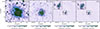 |
Fig. 2. Left: Total intensity map at 1.28 GHz of NGC 1487 with a noise level σI of 4 μJy/beam observed with MeerKAT. Middle left: Total intensity map at 2.1 GHz of NGC 1487 with a noise level σI of 8 μJy/beam observed with ATCA. Middle right: Total intensity map at 5.5 GHz of NGC 1487 with a noise level σI of 5.5 μJy/beam observed with ATCA. Right: Total intensity map at 9 GHz of NGC 1487 with a noise level σI of 5.5 μJy/beam observed with ATCA. The overlaid contours of the total intensity start at 3 σ and increase by factor of 2. The resolution of the different maps can be taken from Table 3 and is shown in the bottom left corner. |
3.2. Spectral analysis
3.2.1. Full integrated spectral energy distribution
To cover a broad range of the radio continuum emission, we use the central frequencies 1.28 GHz, 2.1 GHz, 5.5 GHz and 9 GHz and additionally, we split the MeerKAT dataset into six 143 MHz wide sub-bands, ATCA L/S-band into six 341 MHz wide sub-bands, and C- and X-band into each two sub-bands of 683 MHz width. We applied a 3 σ clipping threshold and computed the integrated flux density, summing all emission over its resolved size using RadioFluxTools6, across the individual frequency slices. To ensure the reliability of the measurements, we have to discard one of the MeerKAT slices and one of the ATCA C-band slices, as the quality is too low. But we also incorporate literature data from the GaLactic and Extragalactic All-sky MWA survey eXtended (GLEAM-X) data (Ross et al. 2024), which cover frequencies from 87 MHz to 221 MHz. We also include the Australian SKA Pathfinder (ASKAP) survey, Rapid ASKAP Continuum Survey (RACS-Low) data (McConnell et al. 2020) at 885 MHz. Also, data from the ASKAP Evolutionary Map of the Universe (EMU) main survey (Hopkins et al. 2025) at 943 MHz are used in this study. Furthermore, we use literature data from Grundy et al. (2025). The full values of the flux densities can be found in Appendix B in Table B.1
To study the spectral behavior, we fit several models to the spectral energy distribution to gain insight into the underlying physical processes. For this, we fit different models, explained in Galvin et al. (2016), Grundy et al. (2025) and Taziaux et al. (2026) to the SED, and we find that a mixture of free–free absorption (ffa1) at low frequency, a superposition of free–free emission and synchrotron emission at intermediate frequency (sfg), and a break due to inverse Compton losses at higher frequencies (sic) fits the data best. We call this model ffa1_sfg_sic. The flux density is given by,
 (1)
(1)
where A represents the synchrotron emission, αnth is the non-thermal spectral index, and B is the free–free emission at a given frequency ν0. νb is the break frequency in the spectrum, and Δα represents the change in the non-thermal spectral index due to synchrotron and inverse Compton losses, assuming continuous electron injection from massive star formation.
At low radio frequencies, synchrotron emission can be attenuated by free-free absorption. This occurs when the synchrotron-emitting regions are embedded within or behind optically thick ionised gas, which absorbs some of the radiation and produces a spectral turnover or flattening, often observed in star-forming galaxies (e.g. Gajović et al. 2025, 2024; Grundy et al. 2025; Taziaux et al. 2025). The strength of this absorption depends on the density and distribution of the ionised gas, and the optical depth τ reaches unity at a characteristic ‘turnover’ frequency. At high frequencies, the spectrum may exhibit further steepening due to energy losses of CREs, primarily via synchrotron radiation and inverse Compton scattering with cosmic microwave background. This results in a gradual steepening of the synchrotron spectral index above a characteristic ‘break’ frequency νb.
In Fig. 3, we show the spectral energy distribution of NGC 1487 using a non-linear least-squares method (leastsq) with six free parameters in the best-fitting model (lffa1_sfg_sic). The fit yields a reduced chi-square of χred2 = 1.10, indicating a statistically acceptable match to the data. Parameter uncertainties were estimated from the fit itself and supplemented with Monte-Carlo sampling to ensure physically meaningful variations (e.g. positive amplitudes and characteristic frequencies). The non-thermal spectral index is αnth = −0.678 ± 0.085, consistent with a moderately steep spectrum indicative of aged CREs. The spectral break occurs at νb ≈ 6.2 ± 1.3 GHz, marking the frequency where synchrotron and inverse Compton losses begin to steepen the spectrum. All the parameter values and its uncertainties are shown in Table. B.2 in Appendix B.
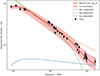 |
Fig. 3. Spectral energy distribution of NGC 1487. The plot displays total intensity data with different observations: GLEAM-X data (Ross et al. 2024), RACS-Low data (McConnell et al. 2020), ASKAP EMU main survey (Hopkins et al. 2025), MeerKAT 1.28 GHz data, ATCA L/S-band, C-band, and X-band data presented in this work, and further data from the work of Grundy et al. (2025). We show the best-fit in red with 1σ uncertainty sampled by EMCEE. The blue, orange, and green dotted lines represent the different components of the best-fit model. |
3.2.2. Pixel-based spectral index
Spectral indices derived from observed total intensity radio continuum emission maps serve as crucial information for explaining the underlying emission mechanisms, and energy loss/gain processes of the synchrotron emitting CREs spatially. We present in Fig. 4, the total spectral index maps of NGC 1487. To minimise additional uncertainties, we do not apply a thermal correction to the maps.
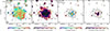 |
Fig. 4. Inband total spectral index of the MeerKAT L-band (panel a)) and its uncertainty (panel b)) between the frequencies 0.96 and 1.59 GHz overlaid with radio emission at frequency of 1.28 GHz starting at 3σ and increase by a factor of 2 (σ = 9 μJy/beam). The resolution of 12″ is shown in the bottom left corner. Two-point total spectral index (panel c)) and its uncertainty (panel d)) between ATCA L/S-band (2.1 GHz) and C-band (5.5 GHz) overlaid with radio emission at frequency of 2.1 GHz starting at 3σ and increase by a factor of 2 (σ = 11.3 μJy/beam). The resolution of 7″ is shown in the bottom left corner. |
To obtain the spatially resolved in-band spectral index, we fit a single power-law spectrum to the flux density in each pixel across the available sub-bands. Panels a) and b) of Fig. 4 show the resulting MeerKAT in-band spectral index map and its associated uncertainty. For this purpose, we split the measurement set into six sub-bands (0.96, 1.09, 1.22, 1.34, 1.47, and 1.59 GHz), convolved each sub-band image to a common resolution of 12″, clipped each map at a noise level of 3σ, and then performed a linear fit in log S − log ν space for every pixel. In the centre of the dwarf galaxy, we find spectral index values reaching up to −0.45 ± 0.02, and it seems that overall they steepen radially towards the edges of the galaxy. But, the map reveals a clear substructure beyond a simple monotonic radial trend. Several compact regions within the disk exhibit flatter spectra compared to their surroundings, most notably towards the western and northeastern parts of the system, following the emission from the Hα map (see middle panel of Fig. 1), which could trace sites of recent CRE injection, similar to IC 10 (Basu et al. 2017b). In contrast, more extended patches of steep spectral index (α ≲ −1) are present towards the southern and northern periphery, suggesting enhanced energy losses or efficient transport of CREs out of the star-forming disk. The spectral index distribution is therefore not azimuthally symmetric due to a combination of spatially intermittent regions of CRE injection, non-uniform CRE transport process7, and possibly localised outflows. Note that at the edges of the galaxy, the total spectral index value flattens significantly and even reaches positive values (e.g. 0.37 ± 0.82 in the southeast side of the galaxy), but these are likely artefacts caused by low signal-to-noise.
In the panel c) and d) of Fig. 4, we show the two-point spectral index and its uncertainty map between the ATCA L/S-band (2.1 GHz) and C-band (5.5 GHz). Both maps were convolved to a common resolution of 7″ and clipped at the 3σ level. The spectrum across the two main cores is relatively flat, with values of −0.36 ± 0.18 and −0.42 ± 0.19, and slightly steeper in the eastern core with −0.46 ± 0.29. The flat spectrum closely follows the distribution of H II regions seen in the Hα map. We note that the core spectral indices differ between the MeerKAT inband and the ATCA L/S– and C-band measurements (panel a) and c) of Fig. 4), mainly because no thermal correction has been applied. The thermal fraction at 1.28 GHz is almost negligible, while it becomes more significant at 2.1 GHz and even more at 5.5 GHz (e.g. Parnovsky & Izotova 2018; Hindson et al. 2018). Consequently, the core appears flatter in the ATCA two-point spectral index map due to the contribution of thermal emission at these higher frequencies. Outside the star-forming regions, the spectrum declines rapidly, with very steep values measured just beyond the knots. This steepening suggests strong energy losses of the CREs, likely dominated by inverse Compton cooling or by transport through outflows or galactic winds.
3.3. Region dependent spectral analysis
The GALEX–FUV and Hα maps in Fig. 1 reveal that NGC 1487 consists of several distinct star-forming components, which can be analysed individually. Following the classification of Buzzo et al. (2021), we divide the system into five regions: APC 1, APC 2, and APC 3 correspond to the three main central star-forming knots, while APC 4 and APC 5 trace the base of the southern and northern tidal features, respectively. Fig. 5 shows SEDs for these regions and an Hα image overlaid with the location of the regions. Each dataset was divided into eight sub-bands, and the flux density was measured for each region. Owing to the low signal-to-noise ratio in the X-band, we only show the sub-band measurements for the main core region (APC 2) and the integrated full band measurement for APC 1 and APC 3. For the regions tracing the base of the tidal features, the ATCA X-band data are excluded, as only noise was detected.
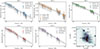 |
Fig. 5. Region dependent spectral energy distribution, showing total and thermal corrected flux density of MeerKAT L-band, ATCA L/S-, C- and X-band data. The bottom right panel shows the Hα map with the individual regions overlaid in different colours. |
To get the synchrotron emission from the total emission we have to apply a thermal correction. Additionally, as starburst dwarf galaxies are generally optically thick (Kepley et al. 2010; Basu et al. 2017b; Taziaux et al. 2025), we also have to account for absorption. It is possible that free–free absorption in a thermal plasma coexists with the relativistic electrons responsible for the synchrotron emission. Therefore, we take internal absorption into account (Tingay & de Kool 2003). Normally, we do not have absorption at these high frequencies, but we still include it in the measurement. We ignore external absorption as we do not expect free–free absorption by a screen of ionised gas located outside the synchrotron emitting region. The thermal correction can be formulated as,
 (2)
(2)
depending on the free–free optical depth τff, the thermal emission S0(ν) which can be obtained by the free–free emission density function in relation to the Hα flux (Deeg et al. 1997, Eq. (3)) and the frequency ν. The full calculation of the thermal correction is detailed in the Appendix A, where we also show that the free–free optical depth τff depends on the electron temperature Te (see Eq. (A.2) in Appendix A). We assume a 10% uncertainty for the total intensity. For the thermal-corrected intensity, we adopt a 20% uncertainty to account for additional factors, including variations in the electron temperature (Te = 10 000 ± 3000 K) and uncertainties in the [N II] line flux correction relative to Hα measurements (Vargas et al. 2018).
For APC 2, the most actively star-forming region (Buzzo et al. 2021), we find a flat spectrum. After removing the thermal contribution, the non-thermal index remains flat (αtot = −0.49 ± 0.02; αnth = −0.52 ± 0.02), which is close to the expected injection index of αinj ≈ −0.5 from diffusive shock acceleration in supernova remnants. In contrast, APC 1 and APC 3 exhibit significantly steeper spectra, with total spectral indices of αtot = −0.73 ± 0.03 and αtot = −0.78 ± 0.03, and non-thermal values of αnth = −0.80 ± 0.03 and αnth = −0.85 ± 0.04, respectively. The steeper spectra in these regions indicate that synchrotron emission dominates and that the CRE population has already experienced radiative losses. This likely means that APC 1 and APC 3 are slightly older star-forming regions compared to APC 2, with fewer newly accelerated electrons. In the regions at the base of the tidal arms, APC 4 and APC 5, we measure steep spectra with total spectral indices of αtot = −0.90 ± 0.03 and αtot = −0.84 ± 0.03, respectively. After correcting for thermal emission, these values become αnth = −0.96 ± 0.03 and αnth = −0.88 ± 0.03. Interestingly, Buzzo et al. (2021) report nearly identical star formation rates for APC 3 and APC 4 (0.04 ± 0.01 M⊙ yr−1 and 0.03 ± 0.01 M⊙ yr−1, respectively).
3.4. Equipartition magnetic field strength
A common approach to estimate the magnetic field strength is to assume equipartition between the energy densities of CRs and the magnetic field, although these assumptions carry significant uncertainties (Pfrommer & Enßlin 2004b; Kepley et al. 2010; Seta & Beck 2019; Ruszkowski & Pfrommer 2023; Dacunha et al. 2025). By assuming that the thermal/non-thermal decomposition is valid and that equipartition can be applied to starburst dwarf galaxies (Chiu et al. 2025), the magnetic field under equipartition can be determined following Beck & Krause (2005)
 (3)
(3)
Here αnth is the non-thermal spectral index and Sν is the synchrotron intensity at the frequency ν. We adopt a proton-to-electron energy density ratio of K0 = 100, in line with values used in previous studies (e.g. Chyży et al. 2016; Basu et al. 2017b; Heesen et al. 2022; Stein et al. 2023; Taziaux et al. 2025). The galaxy inclination is taken as i = 53.4°, and we assume a path length l = 5.5 kpc, corresponding to the spatial extent over which CREs can be traced. Estimating the path length l is generally challenging due to the uncertain geometry of the galaxy. A detailed description of the constants c1, c2, and c4, as well as the full equipartition magnetic field equation, can be found in Beck & Krause (2005). It should be noted that the equipartition formula becomes undefined for simple power-law energy spectra for αnth ≥ −0.5. We use the MeerKAT L-band total intensity map together with the in-band total spectral index map. At 1.28 GHz, the thermal fraction is assumed to be negligible, so no thermal correction is applied.
Fig. 6 shows the equipartition magnetic field strength with strong magnetic field in the centre core with values higher than 12 μG. The strength decreases radially and takes values at the edges of nearly 5 μG. These findings are similar to other dwarf galaxies (e.g. Kepley et al. 2010; Chyży et al. 2016; Basu et al. 2017b; Heesen et al. 2018; Taziaux et al. 2025).
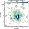 |
Fig. 6. Total magnetic field strength of NGC 1487 estimated assuming energy equipartition between CR particles and magnetic field. The inner white regions are blank where the equipartition condition is invalid (α > −0.5). The overlaid contours are the total intensity emission at 1.28 GHz. |
To calculate the magnetic field strength using the equipartition assumption for the different regions, we use the non-thermal spectral index value for each region and calculate the mean flux value on the MeerKAT L-band map. We still assume the same path length of 5.5 kpc as the physics of the CREs do not change between a small region and the full galaxy. For the more star-forming regions APC 1, APC 2 and APC 3, we calculate a magnetic field strength of 12.67 μG, 18.97 μG, and 11.13 μG, respectively. For the more distant region, APC 4 and APC 5, we calculate a magnetic field strength of 10.12 μG and 5.46 μG.
4. Magnetic field configuration
In the following section, the band names refer to the νref values given in Table 3.
4.1. Polarised emission
In Fig. 7 (MeerKAT L-Band), 8 (ATCA L/S-band), and 9 (ATCA C-band), we present the polarised intensity, fractional polarisation, magnetic field orientations8, and the rotation measure of NGC 1487. To mitigate the strong bias introduced by the positive-definite background, we subtract the background mean (see Table 3) from the polarised intensity map (Heald et al. 2009). To ensure that only significant emission is considered, we apply a clipping threshold of 3 σPI. The noise levels for the polarised intensity σPI were estimated from the bias-corrected polarised intensity map, well separated from the phase centre. As the effective frequency of the polarisation emission map, generated by RM synthesis, is not at the central frequency but at the weighted mean λ02, we normalise the Stokes I to a reference frequency (see Table 3) to generate the fractional polarisation maps /panel b) of Figs. 7–9).
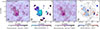 |
Fig. 7. Panel a): Polarised intensity at 1194 MHz with contours starting at 3σPI and increasing by |

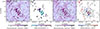 |
Fig. 8. Panel a): Polarised intensity at 2166 MHz with contours starting at 3σPI and increasing by |

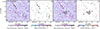 |
Fig. 9. Panel a): Polarised intensity at 5430 MHz with contours starting at 3σPI and increasing by |

In the MeerKAT L-band (Fig. 7), we detect polarised emission in the eastern region of NGC 1487. This polarised emission extends into the continuum disk. Additionally, we observe regions of high polarised intensity below APC 3. The star-forming regions show a relatively low fraction of polarisation (panel b), Fig. 7), which increases towards the galaxy’s outskirts, reaching values of 6–10%. In panel c), we show the magnetic field orientation. At two locations, we also detect extensions where the magnetic-field orientations appear to reach towards the galaxy’s outskirts.
Fig. 8 shows the polarisation properties of the ATCA L/S-band data. We detect polarised emission between the star-forming regions APC 1 and APC 2, as well as around APC 3, which corresponds to the merger. High polarised emission is also observed above APC 3, extending nearly to the outskirts of the galaxy and the beginning of the northern tidal arm. In contrast, lower polarised emission is detected at the start of the southern tidal arm. In panel b) of Fig. 8, the degree of polarisation is low around the star-forming knots, but increases rapidly towards the northern part of the galaxy, reaching nearly 60%. Panel c) shows the magnetic field orientation overlaid on the total intensity. In the northern region, the magnetic field orientations have a similar orientation to those seen in the MeerKAT L-band data and generally point vertically towards the tidal arms. In the central star-forming region, the magnetic field appears chaotic, with orientations pointing in multiple directions and no clear large-scale alignment. This suggests a turbulent magnetic field in the core, influenced by intense star formation and associated gas motions.
Fig. 9 shows the polarisation properties of the ATCA C-band data. Overall, we do not detect significant polarised emission, and the signal is close to the noise level. Only a few small regions show weak polarised emission, primarily along the northern tidal arm. A small detection is also observed on the eastern side of the star-forming region APC 3. For the ATCA X-band data, no polarised emission is detected, so it is not shown here. Although depolarisation is reduced at higher frequencies and one would therefore expect stronger polarised emission, the synchrotron surface brightness, and consequently the polarised intensity, declines steeply with frequency. In our ATCA X-band data, the resulting polarised intensity falls below the noise level, and no significant polarised emission is detected.
4.2. Faraday rotation measure
The rotation measure map in panel d) of Figs. 7, 8, and 9 has been corrected for the Milky Way foreground (Hutschenreuter et al. 2024). The rotation measure value of the Galactic foreground is 3.54 ± 0.92 rad m−2, which is relatively low. Positive values indicate a magnetic field directed towards us, while negative values indicate one pointing away. In the MeerKAT L-band data shown in panel d) of Fig. 7, we observe an overall negative rotation measure as we move into the halo. Near the star-forming regions, there are rapid changes between positive and negative values, however, the relatively low resolution of our data prevents us from fully resolving these quick variations. When analysing the ATCA L/S-band data in Fig. 8, we detect very rapid fluctuations between positive and negative rotation measure values. Within the star-forming cores, depolarisation limits our ability to trace the magnetic field.
However, in the regions between the star-forming knots, the rapid changes in rotation measure suggest the presence of small-scale dynamos. These small-scale dynamos are processes in which turbulent motions of the interstellar gas stretch, twist, and fold magnetic field lines, amplifying the magnetic field locally on short spatial scales (e.g. Beck et al. 2019; Xu & Lazarian 2021; Pfrommer et al. 2022). Unlike large-scale dynamos, which produce coherent fields over kiloparsec scales, small-scale dynamos create tangled, rapidly varying magnetic structures. This could explain the observed quick variations in rotation measure between the star-forming cores, indicating strong, localised magnetic activity. In Fig. 9, we do not observe any significant rotation measure, consistent with the lack of notable magnetic activity in this source.
5. CR transport modelling
CRs in the merging dwarf galaxy system can be accelerated by the shocks generated during the collisions between the interstellar medium (ISM) of interacting galaxies (Lisenfeld & Völk 2010; Hu et al. 2025), and also at the supernova remnant shocks. Transport of CRs specifically through diffusion and advection can influence the SFR and the formation of large-scale galactic wind and shape the radio intensity profile from relativistic CREs (Heesen et al. 2016; Dashyan & Dubois 2020). Therefore, the modelling of CR transport is necessary to probe the insights of magnetic field structure, advection speed and to predict the nature of diffusion processes, whether isotropic or anisotropic, based on the consistency with the observations.
Since 1D modelling (Heald et al. 2022; Stein et al. 2023) neglects the galaxy’s full 3D structure and, in edge-on systems, ignores radial features such as spiral arms, the radial structure of NGC 1487 (inclination i = 53.4°) can still significantly affect the radio emission along the line of sight. Therefore, describing this galaxy in 3D, considering both diffusion and advection, is necessary, especially for an interacting galaxy system due to the presence of highly fluctuating density, velocity, and magnetic field (Hu et al. 2025). We introduce the theoretical study of 3D transport in NGC 1487 by applying publicly available Monte-Carlo code CRPropa (Merten et al. 2017; Alves Batista et al. 2022; Dörner et al. 2023; Aravinthan et al. 2025). Although initially CRPropa9 was developed to perform the transport of ultra-high-energy hadronic CRs by ballistic propagation through the solution of the equation of motion, CRPropa 3.1 is capable of executing simulations in different diffusive environments by solving the transport equation in terms of a stochastic differential equation for the diffusive propagation. The ballistic approach and diffusion module can be used within the same framework as the particle densities in a diffusive scenario can be calculated from the trajectory of pseudo-particles. To model the 3D transport of CR in NGC 1487, we use the diffusion module where the transport equation for CREs can be represented by the diffusion-advection equation,
 (4)
(4)
where n is the particle density distribution, D is the diffusion coefficient, uadv is the advection speed,  is the energy loss and S is the source term, considering the isotropic diffusion. However, recent results (e.g. Kleimann et al. 2025) indicate that diffusion in such systems is likely anisotropic, with diffusion coefficients differing by up to a factor of ∼40 between directions parallel and perpendicular to the magnetic field. Here, the energy loss term represents only synchrotron emission as a continuous process. The modelling of the magnetic field in a merging system like NGC 1487 is complex and the field structure evolves from the pre-merger to the post-merger stage as described in Rodenbeck & Schleicher (2016), Whittingham et al. (2023), Hu et al. (2025) through magneto-hydrodynamic simulations. This differs from the magnetic field of the isolated dwarf galaxy (Siejkowski et al. 2018). The brightest star-forming complexes in NGC 1487 (APC 1, APC 2, and APC 3; Sect. 3.3) trace the locations where the interaction has strongly compressed the ISM. In the absence of direct constraints on the large-scale magnetic-field geometry from previous work, it is reasonable to assume multiple magnetised components originating from progenitor systems. Interacting dwarf galaxies commonly host spiral-like magnetic fields when viewed face-on and X-shaped fields when viewed edge-on (Heesen et al. 2009, 2011; Bera et al. 2019; Stein et al. 2025). The merger-driven overlap and distortion of such components would naturally produce the complex magnetic-field configuration shown in Fig. 10.
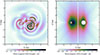 |
Fig. 10. Mean magnetic-field strength maps used as inputs for the CRPropa simulations, shown in face-on (left panel) and edge-on (right panel) projections. The model consists of three logarithmic spiral components centred at APC 1 (0.9 kpc, 0.25 kpc), APC 2 (0.5 kpc, −0.5 kpc), APC 3 (−0.8 kpc, −0.1 kpc) following the star-forming regions identified by Buzzo et al. (2021). A spiral pitch angle of 12° and an X-shaped halo field with an opening angle of 50° are adopted to define the large-scale 3D field structure. |
We place the centre of three spirals at the position of APC 1 (0.9 kpc, 0.25 kpc), APC 2 (0.5 kpc, −0.5 kpc), APC 3 (−0.8 kpc, −0.1 kpc) following Buzzo et al. (2021). We assumed that the spiral field with a pitch angle of 12° and the opening angle of X-shape field is 50° as at these positions star-forming regions are located. We structure the overlapping magnetic field strength in line with the calculated equipartition magnetic field strength at regions APC 1, APC 2, and APC 3 as discussed in Sect. 3.4. We consider the maximum radius of NGC 1487 is 2.75 kpc and particles that reach this boundary exit the simulation volume. Electrons are injected at APC 1, APC 2, APC 3 within the sphere of radius 0.5 kpc, 0.1 kpc, and 0.1 kpc, respectively with an injection spectrum dN/dE ∝ E−γ in the energy range of 0.1 GeV to 50 GeV. At the initial stage, we use a constant diffusion coefficient D = 1028 cm2 s−1, only considering the parallel diffusion and propagating electrons for 0.1 Gyr to achieve the steady state distribution of CREs. From this simplified simulation set up, γ = 2.2 provides the overall non-thermal radio spectral index of αnth = −0.678, found in NGC 1487 (see Sect. 3.2.1), only considering diffusion. If we consider both diffusion and advection with constant uadv = sgn(z) u ez, where u = 160 km s−110, αnth = −0.678 is produced by γ ∼ 2.34 which is close to equilibrium electron spectral index. This is because of the high advection speed; electrons are advected before they can diffuse in the galaxy. This is also reflected in the calculated CRE transport timescales for diffusion and advection (see Eqs. (D.6) and (D.7) in Appendix D). Using the adopted scale height of the synchrotron-emitting region, taken as half the CRE propagation path length (h = 2.75 kpc), diffusion coefficient D, and an escape velocity derived from the rotation velocity (e.g. Heesen et al. 2018), we obtain a diffusion timescale of τdiff = 228.17 Myr and an advection timescale of τadv = 16.72 Myr.
Therefore, an extensive theoretical study is required to analyse the morphology of the radio emission and radio spectral index, yet this is out of the scope of this paper. Considering Kolmogorov turbulence with an anisotropic diffusion model (e.g. Kleimann et al. 2025; Lübke et al. 2025), we show that with the 3D simulation environment of CRPropa, we can use the geometry of the merging galaxies (Hu et al. 2025), including a 3D structure of the magnetic field, to reproduce the spectral behavior as a function of the distance from the disk. This approach for the first time opens up the possibility to study 3D effects of cosmic-ray transport in complex systems like NGC 1487. In future work (Das in prep.), we will be able to investigate the properties of cosmic-ray transport via a detailed comparison of the morphology of the galaxy with the simulations.
6. Discussion
6.1. Energy losses
The spectral break observed at 6.2 ± 1.3 GHz in NGC 1487 in Fig. 3 is consistent with features reported in other starburst dwarf galaxies such as NGC 1569 and NGC 4449 (Klein et al. 2018). This break can be understood as the frequency at which the radiative cooling time of CREs becomes comparable to their escape time from the star-forming regions. At higher frequencies, CREs enter a loss-dominated regime, where they rapidly lose energy through synchrotron radiation and/or inverse-Compton scattering before they can propagate into the halo.
The overall non-thermal spectral index of α ≈ −0.678 (Sν ∝ να) provides an important diagnostic of the underlying CRE population. This index represents the transport-dominated regime below the spectral break. Using the relation α = (γ − 1)/2, we infer a CRE energy spectral index of γ = 2.36 (n(E)∝E−γ). This value is consistent with the initial injection spectrum, and agrees well with the typical injection index of γ ≈ 2.3 inferred from supernova remnants, where diffusive shock acceleration is believed to be the main acceleration process (Ruszkowski & Pfrommer 2023). In the loss-dominated regime, the steady-state CRE spectrum steepens by exactly one power, such that n(E)∝E−(γ + 1). This corresponds to a steepening of the synchrotron spectral index by Δα = 0.5, leading to a cooled spectral index of αcooled = γ/2 ≈ 1.18. Separating the contributions of synchrotron and inverse-Compton losses is challenging, since both scale as Ėe ∝ E2 and thus produce similar spectral steepening. Their relative importance depends on the energy densities of the magnetic field (uB) and the ambient photon field (uph), with inverse-Compton losses dominating when uph > uB. In merger environments like NGC 1487, the far-infrared photon field from dust-reprocessed starlight can be very strong, potentially making inverse-Compton scattering the dominant cooling process. Lacki et al. (2010) showed that in such cases, galaxies may deviate from the linear far-infrared–radio correlation, since efficient inverse-Compton cooling reduces the energy available for synchrotron emission.
This result highlights a key tension with the simple ‘calorimeter’ model. In a pure calorimeter dominated by synchrotron and inverse-Compton losses with an injection index of γ ≈ 2.36, an overall spectral index of α ≈ −1.18 is expected. In contrast, our observed harder spectrum of α = −0.678 indicates that the calorimeter model does not apply globally in NGC 1487. The relatively hard spectrum shows that many CREs avoid significant radiative cooling inside the galaxy. This suggests that escape mechanisms, such as diffusion or streaming along magnetic field structures, play a major role in regulating the radio continuum output of this interacting system. An additional explanation arises from the galaxy’s star formation history (Buzzo et al. 2021), recent and bursty star formation episodes in APC 1, 2 and 3, inject a substantial population of high-energy electrons on timescales shorter than the effective cooling time. The resulting radio continuum is therefore a mixture of freshly accelerated electrons near star-forming regions and partially cooled electrons undergoing local escape, which together prevent the spectrum from steepening to calorimeter predictions (e.g. Ruszkowski & Pfrommer 2023).
To quantify the relative contributions of radiative losses and escape, we compute the CRE cooling times following Werhahn et al. (2021), Taziaux et al. (2025) and Basu et al. (2015), considering synchrotron, inverse-Compton, and bremsstrahlung losses. A detailed explanation of the CRE timescale equations is provided in Appendix D. We ignore the timescale for Coulomb losses, as they are primarily effective at lower CRE energies and are largely irrelevant at the higher energies associated with synchrotron-emitting CREs (Petrosian 2001; Ruszkowski & Pfrommer 2023). We adopt an observing frequency of 1.28 GHz and a magnetic field strength of 12 μG.
Following Eq. (D.1) in Appendix D, we derive a characteristic electron energy of Ee = 2.58 GeV. The synchrotron cooling timescale of the CREs is calculated using Eq. (D.2), yielding τsyn = 22.47 Myr. Inverse Compton losses are estimated by considering both the interstellar radiation field in the dwarf galaxy and the cosmic microwave background (CMB). Adopting energy densities of Urad = 5.73 × 10⁻¹² erg cm−3 calculated from the magnetic energy density (Heesen et al. 2014) and UCMB = 4.2 × 10⁻¹³ erg cm−3 (Heesen et al. 2018), we obtain an inverse Compton cooling timescale of τIC = 28.36 Myr. Bremsstrahlung losses are computed assuming a neutral gas electron density of ne = 0.5 cm−3, representative of the diffuse ISM in dwarf galaxies following Eq. (D.4) in Appendix D. This results in a Bremsstrahlung timescale of τbrem = 79.2 Myr. Combining all radiative loss processes (see Eq. (D.5) in Appendix D), the total cooling timescale of the CRE population is found to be τcool = 10.59 Myr. We compare this value with the CRE escape timescale, assuming advection is the dominant transport process, which is estimated to be τesc = τadv = 16.72 Myr. Furthermore, an older independent estimate of the CRE lifetime is obtained from spectral ageing. A spectral break is observed at νbrk = 6.2 GHz (Fig. 3). Using the Jaffe-Perola ageing model (Hughes 1991), which assumes continuous isotropisation of electron pitch angles, we derive a spectral age of τspec = 14.3 Myr following Eq. (D.8). This timescale represents the time elapsed since the most recent injection of freshly accelerated CREs (Heesen et al. 2014).
The comparison of the characteristic timescales indicates that radiative losses dominate the CRE evolution. The total cooling time (τcool ≈ 10.6 Myr) is shorter than both the escape time (τesc ≈ 16.7 Myr) and the spectral age (τspec ≈ 14.3 Myr), implying that CREs lose a significant fraction of their energy before escaping the system. Synchrotron and inverse Compton losses are the dominant cooling processes, reflecting the combined influence of the magnetic field and radiation field energy densities, while Bremsstrahlung losses are negligible due to the low gas density. The agreement between the cooling timescale and the spectral age supports a radiative origin of the spectral break at 6.2 GHz and validates the use of the Jaffe-Perola ageing model. The resulting timescales further indicate that large-scale CRE escape via galactic winds is inefficient, and that the observed radio emission is dominated by synchrotron-regulated cooling. The galaxy therefore behaves as an approximate, though not perfect, CRE calorimeter at GHz frequencies, with escape and local transport processes contributing at a secondary level.
6.2. Role of the magnetic field
6.2.1. Small-scale dynamo in galaxy core
The rapid fluctuations in RM observed in the star-forming knots of NGC 1487 strongly suggest that the magnetic field there is dominated by turbulent, small-scale structures. Such variability is a trend of the small-scale dynamo, which produces a tangled field amplified on the scales of turbulent driving, rather than the coherent, ordered fields expected from a large-scale dynamo (Beck et al. 2019). In this system, the small-scale dynamo is likely powered by the intense turbulence generated during the merger-driven starburst, where stellar winds and overlapping supernova explosions inject kinetic energy into the ISM.
The efficiency of this process is demonstrated in other dwarfs. In IC 10, the magnetic field strength correlates with the star formation rate as B ∝ SFR0.35 (Basu et al. 2017b), consistent with fluctuation dynamo predictions. In NGC 1569, the magnetic morphology is directly tied to supernova-driven Hα bubbles, again indicating amplification through turbulence (Kepley et al. 2010). These observations confirm that in starbursting dwarfs, where turbulence dominates gas dynamics, the small-scale dynamo provides the primary mechanism for magnetic field growth.
The implications are twofold. Dwarf galaxies such as NGC 1487 are close analogues of high-redshift systems, where small-scale dynamos rapidly amplify seed fields to significant strengths within ∼10 Myr, ensuring early magnetisation (Schleicher et al. 2010; Rieder & Teyssier 2017). At later stages, this turbulent amplification provides the seed for large-scale dynamo action, which organises the field once rotation and stratification dominate (Elstner et al. 2014). Simulations indicate, however, that strong small-scale activity can delay large-scale ordering, extending its growth from ∼1 − 2 Gyr to > 5 Gyr (Schleicher et al. 2010; Rieder & Teyssier 2017).
In this context, the RM variability in NGC 1487 is not only evidence of ongoing small-scale dynamo action, but also a snapshot of the transitional phase in galaxy assembly. Starburst-driven turbulence amplifies and sustains magnetic fields in dwarfs, while mergers and outflows transport these tangled fields into the circumgalactic medium, contributing to the magnetisation of the larger systems that these dwarfs eventually form.
6.2.2. Magnetic field orientation in the tidal arms
In Fig. 11, we present the Hα map with the overlaid magnetic field orientations derived from the different observations. The magnetic field vectors clearly extend into the tidal arm of this dwarf–dwarf merger system. We identify two main regions of interest, corresponding to the magnetic field orientations observed with MeerKAT L-band (point A in Fig. 11) and ATCA C-band (point B in Fig. 11). The figure shows that, after a rather chaotic field configuration in the central region of the galaxy, the magnetic field becomes more ordered and points roughly northward, towards the base of the tidal arm (as seen in the ATCA L/S-band data). Along the tidal arm, the field continues to align with the structure, reaching points B and A towards the outer end of the arm. Additionally, at points C and D in Fig. 11, the magnetic field vectors are directed towards the outer regions of the galaxy, curving slightly into the halo. This curvature suggests the presence of a large-scale magnetic field structure. These magnetic field loops are also in agreement with the simulation presented in Fig. 10. At point D, the field appears to follow the tidal arm while bending outward, again indicating a possible magnetic loop extending into the halo.
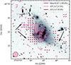 |
Fig. 11. Hα map with overlaid magnetic field orientation of the MeerKAT L-band data (in red), ATCA L/S-band data (in pink) and ATCA 5.5 GHz data (in brown). The corresponding resolution is shown in bottom left corner. |
Similar results were reported by Basu et al. (2017a), who detected ordered magnetic fields in the tidal tail of an interacting galaxy system, the Antennae galaxies. Their study showed that tidal interactions can compress and shear the ISM, which helps to align and strengthen the magnetic field on large scales. These findings, together with our results, suggest that tidal forces in galaxy mergers play an important role in shaping and maintaining large-scale magnetic field structures. Such fields can stay coherent over several kiloparsecs and are visible as polarised synchrotron emission even in the outer regions of the interacting galaxies.
7. Conclusion
This study presents a comprehensive study, and the first radio continuum polarimetry study, of the dwarf–dwarf merger NGC 1487 to date. The key aspects of the study focused on investigating the magnetic field structure, CR transport, and energy loss mechanisms within this low-mass merging system using multi-band radio continuum data from MeerKAT (L-band) and ATCA (L/S-, C-, and X-bands). These can be summarised under the following points.
-
Radio continuum emission is detected all over the frequency range and is even traced in the tidal arms at MeerKAT L-band. The overall non-thermal spectral index derived from the full integrated SED is αnth = −0.678 ± 0.085, consistent with an aged CRE population.
-
The SED analysis revealed that the best-fit model (ffa1_sfg_sic) includes free–free absorption at low frequencies, synchrotron/free–free emission, and a break due to inverse Compton losses at higher frequencies. A spectral break frequency νb ≈ 6.2 ± 1.3 GHz was observed. This break suggests that at frequencies above this point, CREs enter a loss-dominated regime where radiative cooling time is comparable to the escape time.
-
Region-dependent spectral analysis shows that actively star-forming knots (e.g. APC 2) exhibit relatively flat non-thermal spectra (αnth = −0.52 ± 0.02). In contrast, regions located at the base of the tidal arms (e.g. APC 4) have significantly steeper non-thermal spectra (αnth = −0.96 ± 0.03), indicating that the CREs in these outer regions have experienced substantial radiative losses or more efficient transport and escape.
-
Calculations comparing cooling and escape timescales indicate that the CRE cooling time at 1.28 GHz (τcool ≈ 10.6 Myr) is comparable to the estimated escape time via advection in a galactic wind (τesc ∼ 16.7 Myr). This suggests that radiative losses are important in regulating the CRE population, but that escape processes also play a significant role. While synchrotron losses are somewhat more efficient than inverse-Compton losses under the adopted conditions, the relatively flat observed radio spectral index (α = −0.68) compared to the expectation for a pure electron calorimeter (α ≈ −1.18) indicates that a substantial fraction of CREs escape before losing all of their energy. The galaxy therefore does not behave as a perfect electron calorimeter; instead, its radio emission reflects a balance between radiative cooling and CRE transport.
-
Within the star-forming knots, rapid fluctuations in RM were observed. These fluctuations strongly suggest that the core magnetic field is dominated by turbulent, small-scale structures generated by the small-scale dynamo, likely powered by intense merger-driven turbulence.
-
Outside the chaotic core, the magnetic field orientations clearly extend and align with the tidal arms, pointing roughly northward towards the base of the tidal arm. This result, consistent with the findings in other interacting galaxies (Basu et al. 2017a), indicates that tidal forces play an important role in shaping and maintaining large-scale magnetic field structures in merging dwarf galaxies.
Data availability
A copy of the reduced images are available at the CDS via https://cdsarc.cds.unistra.fr/viz-bin/cat/J/A+A/708/A212
Acknowledgments
ST, CJR, DJB, MS, JBT, SD, and RJD acknowledge the support from the DFG via the Collaborative Research Center SFB1491 Cosmic Interacting Matters - From Source to Signal (project no. 445052434). PK acknowledges the support of the BMBF project 05A23PC1 for D-MeerKAT. The MeerKAT telescope is operated by the South African Radio Astronomy Observatory, which is a facility of the National Research Foundation, an agency of the Department of Science and Innovation. The Australia Telescope Compact Array is part of the Australia Telescope National Facility (https://ror.org/05qajvd42), which is funded by the Australian Government for operation as a National Facility managed by CSIRO. We acknowledge the Gomeroi people as the Traditional Owners of the Observatory site. We acknowledge data storage and computational facilities by the University of Bielefeld, which are hosted by the Forschungszentrum Jülich and were funded by German Federal Ministry of Education and Research (BMBF) projects D-LOFAR IV (05A17PBA) and D-MeerKAT-II (05A20PBA), as well as technical and operational support by BMBF projects D-LOFAR 2.0 (05A20PB1) and D-LOFAR-ERIC (05A23PB1), and German Research Foundation (DFG) project PUNCH4NFDI (460248186). The Legacy Survey team makes use of data products from the Near-Earth Object Wide-field Infrared Survey Explorer (NEOWISE), which is a project of the Jet Propulsion Laboratory/California Institute of Technology. NEOWISE is funded by the National Aeronautics and Space Administration. The Legacy Surveys imaging of the DESI footprint is supported by the Director, Office of Science, Office of High Energy Physics of the U.S. Department of Energy under Contract No. DE-AC02-05CH1123, by the National Energy Research Scientific Computing Center, a DOE Office of Science User Facility under the same contract; and by the U.S. National Science Foundation, Division of Astronomical Sciences under Contract No. AST-0950945 to NOAO.
References
- Aguero, E. L., & Paolantonio, S. 1997, AJ, 114, 102 [Google Scholar]
- Alves Batista, R., Becker Tjus, J., Dörner, J., et al. 2022, JCAP, 2022, 035 [CrossRef] [Google Scholar]
- Aravinthan, A., Dörner, J., Becker Tjus, J., et al. 2025, arXiv e-prints [arXiv:2509.19458] [Google Scholar]
- Basu, A., Beck, R., Schmidt, P., & Roy, S. 2015, MNRAS, 449, 3879 [NASA ADS] [CrossRef] [Google Scholar]
- Basu, A., Mao, S. A., Kepley, A. A., et al. 2017a, MNRAS, 464, 1003 [NASA ADS] [CrossRef] [Google Scholar]
- Basu, A., Roychowdhury, S., Heesen, V., et al. 2017b, MNRAS, 471, 337 [NASA ADS] [CrossRef] [Google Scholar]
- Beck, R., & Krause, M. 2005, Astron. Nachr., 326, 414 [Google Scholar]
- Beck, R., & Wielebinski, R. 2013, in Planets, Stars and Stellar Systems. Volume 5: Galactic Structure and Stellar Populations, eds. T. D. Oswalt, & G. Gilmore, 5, 641 [NASA ADS] [Google Scholar]
- Beck, R., Chamandy, L., Elson, E., & Blackman, E. G. 2019, Galaxies, 8, 4 [NASA ADS] [CrossRef] [Google Scholar]
- Bera, P., Shukurov, A., & Subramanian, K. 2019, Galaxies, 7, 91 [Google Scholar]
- Bergvall, N., & Johansson, L. 1995, A&AS, 113, 499 [NASA ADS] [Google Scholar]
- Breitschwerdt, D., McKenzie, J. F., & Voelk, H. J. 1991, A&A, 245, 79 [NASA ADS] [Google Scholar]
- Brentjens, M. A., & de Bruyn, A. G. 2005, A&A, 441, 1217 [NASA ADS] [CrossRef] [EDP Sciences] [Google Scholar]
- Burn, B. J. 1966, MNRAS, 133, 67 [Google Scholar]
- Buzzo, M. L., Ziegler, B., Amram, P., et al. 2021, MNRAS, 503, 106 [NASA ADS] [CrossRef] [Google Scholar]
- Chiu, H. H. S., Ruszkowski, M., Werhahn, M., Pfrommer, C., & Thomas, T. 2025, A&A, submitted [arXiv:2510.03229] [Google Scholar]
- ChyŻy, K. T., Beck, R., Kohle, S., Klein, U., & Urbanik, M. 2000, A&A, 355, 128 [Google Scholar]
- Chyży, K. T., Drzazga, R. T., Beck, R., et al. 2016, ApJ, 819, 39 [CrossRef] [Google Scholar]
- Dacunha, T., Martin-Alvarez, S., Clark, S. E., & Lopez-Rodriguez, E. 2025, ApJ, 980, 197 [Google Scholar]
- Dashyan, G., & Dubois, Y. 2020, A&A, 638, A123 [EDP Sciences] [Google Scholar]
- Deeg, H.-J., Duric, N., & Brinks, E. 1997, A&A, 323, 323 [NASA ADS] [Google Scholar]
- Dörner, J., Reichherzer, P., Becker Tjus, J., & Heesen, V. 2023, A&A, 669, A111 [NASA ADS] [CrossRef] [EDP Sciences] [Google Scholar]
- Elstner, D., Beck, R., & Gressel, O. 2014, A&A, 568, A104 [NASA ADS] [CrossRef] [EDP Sciences] [Google Scholar]
- Gajović, L., Adebahr, B., Basu, A., et al. 2024, A&A, 689, A68 [NASA ADS] [CrossRef] [EDP Sciences] [Google Scholar]
- Gajović, L., Heesen, V., Brüggen, M., et al. 2025, A&A, 695, A41 [NASA ADS] [CrossRef] [EDP Sciences] [Google Scholar]
- Galvin, T. J., Seymour, N., Filipović, M. D., et al. 2016, MNRAS, 461, 825 [Google Scholar]
- Girichidis, P., Naab, T., Walch, S., et al. 2016, ApJ, 816, L19 [NASA ADS] [CrossRef] [Google Scholar]
- Grundy, J. A., Seymour, N., Wong, O. I., et al. 2025, PASA, 42, e002 [Google Scholar]
- Heald, G., Braun, R., & Edmonds, R. 2009, A&A, 503, 409 [NASA ADS] [CrossRef] [EDP Sciences] [Google Scholar]
- Heald, G. H., Heesen, V., Sridhar, S. S., et al. 2022, MNRAS, 509, 658 [Google Scholar]
- Heesen, V., Beck, R., Krause, M., & Dettmar, R.-J. 2009, A&A, 494, 563 [CrossRef] [EDP Sciences] [Google Scholar]
- Heesen, V., Rau, U., Rupen, M. P., Brinks, E., & Hunter, D. A. 2011, ApJ, 739, L23 [NASA ADS] [CrossRef] [Google Scholar]
- Heesen, V., Croston, J. H., Harwood, J. J., Hardcastle, M. J., & Hota, A. 2014, MNRAS, 439, 1364 [Google Scholar]
- Heesen, V., Dettmar, R.-J., Krause, M., Beck, R., & Stein, Y. 2016, MNRAS, 458, 332 [NASA ADS] [CrossRef] [Google Scholar]
- Heesen, V., Krause, M., Beck, R., et al. 2018, MNRAS, 476, 158 [CrossRef] [Google Scholar]
- Heesen, V., Rafferty, D. A., Horneffer, A., et al. 2018, MNRAS, 476, 1756 [NASA ADS] [CrossRef] [Google Scholar]
- Heesen, V., Staffehl, M., Basu, A., et al. 2022, A&A, 664, A83 [NASA ADS] [CrossRef] [EDP Sciences] [Google Scholar]
- Henkel, C., Hunt, L. K., & Izotov, Y. I. 2022, Galaxies, 10, 11 [NASA ADS] [CrossRef] [Google Scholar]
- Hindson, L., Kitchener, G., Brinks, E., et al. 2018, ApJS, 234, 29 [NASA ADS] [CrossRef] [Google Scholar]
- Högbom, J. A. 1974, A&AS, 15, 417 [Google Scholar]
- Hopkins, A., Kapinska, A., Marvil, J., et al. 2025, PASA, 42, e071 [Google Scholar]
- Hu, Y., Whittingham, J., Lazarian, A., et al. 2025, ApJ, 983, 32 [Google Scholar]
- Hughes, P. A. 1991, Beams and Jets in Astrophysics (Cambridge University Press) [Google Scholar]
- Hutschenreuter, S., Haverkorn, M., Frank, P., Raycheva, N. C., & Enßlin, T. A. 2024, A&A, 690, A314 [NASA ADS] [CrossRef] [EDP Sciences] [Google Scholar]
- Kepley, A. A., Mühle, S., Everett, J., et al. 2010, ApJ, 712, 536 [Google Scholar]
- Kepley, A. A., Zweibel, E. G., Wilcots, E. M., Johnson, K. E., & Robishaw, T. 2011, ApJ, 736, 139 [Google Scholar]
- Kleimann, J., Fichtner, H., Stein, M., et al. 2025, A&A, 699, A92 [NASA ADS] [CrossRef] [EDP Sciences] [Google Scholar]
- Klein, U., Lisenfeld, U., & Verley, S. 2018, A&A, 611, A55 [NASA ADS] [CrossRef] [EDP Sciences] [Google Scholar]
- Kronberg, P. P. 2016, Magnetic Field Outflow from Dwarf and Starburst Galaxies, Cambridge Astrophysics (Cambridge University Press), 100 [Google Scholar]
- Kulsrud, R., & Pearce, W. P. 1969, ApJ, 156, 445 [NASA ADS] [CrossRef] [Google Scholar]
- Lacki, B. C., Thompson, T. A., & Quataert, E. 2010, ApJ, 717, 1 [Google Scholar]
- Lemmerz, R., Shalaby, M., Pfrommer, C., & Thomas, T. 2025, ApJ, 979, 34 [Google Scholar]
- Lisenfeld, U., & Völk, H. J. 2010, A&A, 524, A27 [NASA ADS] [CrossRef] [EDP Sciences] [Google Scholar]
- Lübke, J., Effenberger, F., Wilbert, M., Fichtner, H., & Grauer, R. 2025, arXiv e-prints [arXiv:2509.15320] [Google Scholar]
- McConnell, D., Hale, C. L., Lenc, E., et al. 2020, PASA, 37, e048 [Google Scholar]
- McMullin, J. P., Waters, B., Schiebel, D., Young, W., & Golap, K. 2007, ASP Conf. Ser., 376, 127 [Google Scholar]
- Mengel, S., Lehnert, M. D., Thatte, N. A., et al. 2008, A&A, 489, 1091 [NASA ADS] [CrossRef] [EDP Sciences] [Google Scholar]
- Merten, L., Becker Tjus, J., Fichtner, H., Eichmann, B., & Sigl, G. 2017, JCAP, 2017, 046 [CrossRef] [Google Scholar]
- Meurer, G. R., Hanish, D. J., Ferguson, H. C., et al. 2007, VizieR On-line Data Catalog: J/ApJS/165/307 [Google Scholar]
- Mićić, M., Holmes, O. J., Wells, B. N., & Irwin, J. A. 2022, ApJ, 944, 160 [Google Scholar]
- Moshir, M., Copan, G., Conrow, T., et al. 1993, VizieR Online Data Catalog: IRAS Faint Source Catalog, |b| > 10, Version 2.0 (Moshir+ 1989) [Google Scholar]
- Oey, M. S., Meurer, G. R., Yelda, S., et al. 2007, ApJ, 661, 801 [NASA ADS] [CrossRef] [Google Scholar]
- Offringa, A. R., McKinley, B., Hurley-Walker, N., et al. 2014, MNRAS, 444, 606 [Google Scholar]
- Pakmor, R., Pfrommer, C., Simpson, C. M., & Springel, V. 2016, ApJ, 824, L30 [NASA ADS] [CrossRef] [Google Scholar]
- Pakmor, R., Guillet, T., Pfrommer, C., et al. 2018, MNRAS, 481, 4410 [Google Scholar]
- Papaderos, P., Recchi, S., & Hensler, G. 2012, in Dwarf galaxies: Keys to galaxy formation and evolution proceedings of Symposium 3 of JENAM 2010, (Springer), Astrophysics and space science proceedings [Google Scholar]
- Parnovsky, S., & Izotova, I. 2018, Bulletin of Taras Shevchenko National University of Kyiv. Astronomy, 57, 41 [Google Scholar]
- Perley, R. A., & Butler, B. J. 2013, ApJS, 206, 16 [Google Scholar]
- Petrosian, V. 2001, ApJ, 557, 560 [Google Scholar]
- Pfrommer, C., & Enßlin, T. A. 2004a, A&A, 413, 17 [NASA ADS] [CrossRef] [EDP Sciences] [Google Scholar]
- Pfrommer, C., & Enßlin, T. A. 2004b, MNRAS, 352, 76 [NASA ADS] [CrossRef] [Google Scholar]
- Pfrommer, C., Pakmor, R., Schaal, K., Simpson, C. M., & Springel, V. 2017a, MNRAS, 465, 4500 [NASA ADS] [CrossRef] [Google Scholar]
- Pfrommer, C., Pakmor, R., Simpson, C. M., & Springel, V. 2017b, ApJ, 847, L13 [NASA ADS] [CrossRef] [Google Scholar]
- Pfrommer, C., Werhahn, M., Pakmor, R., Girichidis, P., & Simpson, C. M. 2022, MNRAS, 515, 4229 [NASA ADS] [CrossRef] [Google Scholar]
- Purcell, C. R., Van Eck, C. L., West, J., Sun, X. H., & Gaensler, B. M. 2020, Astrophysics Source Code Library [record ascl:2005.003] [Google Scholar]
- Recchia, S., Blasi, P., & Morlino, G. 2017, MNRAS, 470, 865 [Google Scholar]
- Reissl, S., Klessen, R. S., Pellegrini, E. W., et al. 2023, Nat. Astron., 7, 1295 [Google Scholar]
- Rieder, M., & Teyssier, R. 2017, MNRAS, 472, 4368 [NASA ADS] [CrossRef] [Google Scholar]
- Rodenbeck, K., & Schleicher, D. R. G. 2016, A&A, 593, A89 [NASA ADS] [CrossRef] [EDP Sciences] [Google Scholar]
- Rodruck, M., Charlton, J., Borthakur, S., et al. 2023, MNRAS, 526, 2341 [Google Scholar]
- Ross, K., Hurley-Walker, N., Galvin, T. J., et al. 2024, PASA, 41, e054 [NASA ADS] [CrossRef] [Google Scholar]
- Ruszkowski, M., & Pfrommer, C. 2023, A&ARv, 31, 4 [NASA ADS] [CrossRef] [Google Scholar]
- Sault, R. J., Teuben, P. J., & Wright, M. C. H. 1995, ASP Conf. Ser., 77, 433 [NASA ADS] [Google Scholar]
- Schleicher, D. R. G., & Beck, R. 2013, A&A, 556, A142 [NASA ADS] [CrossRef] [EDP Sciences] [Google Scholar]
- Schleicher, D. R. G., Banerjee, R., Sur, S., et al. 2010, A&A, 522, A115 [NASA ADS] [CrossRef] [EDP Sciences] [Google Scholar]
- Seta, A., & Beck, R. 2019, Galaxies, 7, 45 [NASA ADS] [CrossRef] [Google Scholar]
- Shalaby, M., Thomas, T., & Pfrommer, C. 2021, ApJ, 908, 206 [Google Scholar]
- Shalaby, M., Thomas, T., Pfrommer, C., Lemmerz, R., & Bresci, V. 2023, J. Plasma Phys., 89, 175890603 [Google Scholar]
- Siejkowski, H., Soida, M., & Chyży, K. T. 2018, A&A, 611, A7 [NASA ADS] [CrossRef] [EDP Sciences] [Google Scholar]
- Smoot, G. F. 1998, arXiv e-prints [arXiv:astro-ph/9801121] [Google Scholar]
- Stein, Y., Dettmar, R. J., Weżgowiec, M., et al. 2019, A&A, 632, A13 [NASA ADS] [CrossRef] [EDP Sciences] [Google Scholar]
- Stein, M., Heesen, V., Dettmar, R. J., et al. 2023, A&A, 670, A158 [NASA ADS] [CrossRef] [EDP Sciences] [Google Scholar]
- Stein, M., Kleimann, J., Adebahr, B., et al. 2025, A&A, 696, A112 [NASA ADS] [CrossRef] [EDP Sciences] [Google Scholar]
- Strong, A. W., Moskalenko, I. V., & Ptuskin, V. S. 2007, Ann. Rev. Nucl. Part. Sci., 57, 285 [NASA ADS] [CrossRef] [Google Scholar]
- Taziaux, S., Müller, A., Adebahr, B., et al. 2025, A&A, 696, A226 [NASA ADS] [CrossRef] [EDP Sciences] [Google Scholar]
- Taziaux, S., Johnson, M. C., Shuvo, O. I., et al. 2026, A&A, 706, A90 [NASA ADS] [CrossRef] [EDP Sciences] [Google Scholar]
- Thomas, T., & Pfrommer, C. 2019, MNRAS, 485, 2977 [NASA ADS] [CrossRef] [Google Scholar]
- Thomas, T., Pfrommer, C., & Enßlin, T. 2020, ApJ, 890, L18 [Google Scholar]
- Thomas, T., Pfrommer, C., & Pakmor, R. 2023, MNRAS, 521, 3023 [NASA ADS] [CrossRef] [Google Scholar]
- Tingay, S. J., & de Kool, M. 2003, AJ, 126, 723 [Google Scholar]
- Uhlig, M., Pfrommer, C., Sharma, M., et al. 2012, MNRAS, 423, 2374 [CrossRef] [Google Scholar]
- Vargas, C. J., Mora-Partiarroyo, S. C., Schmidt, P., et al. 2018, ApJ, 853, 128 [NASA ADS] [CrossRef] [Google Scholar]
- Vorontsov-Velyaminov, B. A. 1959, Atlas and Catalog of Interacting Galaxies, 0 [Google Scholar]
- Wardle, J. F. C., & Kronberg, P. P. 1974, ApJ, 194, 249 [Google Scholar]
- Werhahn, M., Pfrommer, C., & Girichidis, P. 2021, MNRAS, 508, 4072 [NASA ADS] [CrossRef] [Google Scholar]
- Werhahn, M., Girichidis, P., Pfrommer, C., & Whittingham, J. 2023, MNRAS, 525, 4437 [Google Scholar]
- Whittingham, J., Sparre, M., Pfrommer, C., & Pakmor, R. 2023, MNRAS, 526, 224 [NASA ADS] [CrossRef] [Google Scholar]
- Xu, S., & Lazarian, A. 2021, Rev. Mod. Plasma Phys., 5, 2 [Google Scholar]
- Zweibel, E. G. 2013, Phys. Plasmas, 20, 055501 [NASA ADS] [CrossRef] [Google Scholar]
The corresponding technical keyword in miriad is mfboot.
Peak polarised intensity after Ricean-bias correction, applied when snrPIfit > 5, using  .
.
Non-uniform CRE transport denotes possible spatial variations in diffusion/advection and energy-loss conditions that cause CREs to propagate differently across the galaxy.
Throughout this work, ‘magnetic field orientations’ refers to Faraday rotation corrected magnetic field orientations.
calculated using the rotation velocity  (Heesen et al. 2018).
Appendix A: Calculations for thermal correction
Follow Eq 2, we can determine the thermal emission S0(ν) by using the Hα emission as its tracer, because it originates from the recombination of the same free electrons that produces the free–free emission. Therefore, we use the free–free emission S0 developed by Deeg et al. (1997) to use as thermal emission subtraction.
 (A.1)
(A.1)
To take into account the internal absorption in NGC 1487, we use the free–free optical depth τff defined as
 (A.2)
(A.2)
while the emission measure EM is directly related to the Hα flux density.
 (A.3)
(A.3)
With the solid angle Ω, we can transform from steradian to the integrated Hα emission with knowing that 1 sr = 4.25 × 10¹⁰ arcsec2. Therefore, we can use  (Smoot 1998) where θ is the angular radius in arcsec, we get
 (A.4)
(A.4)
Appendix B: Radio flux densities
In this section, we present the values for the radio flux densities of the MeerKAT, ATCA and the literature data in Table B.1. In Table B.2, we show the exact parameter values and its uncertainties of the best-fit model.
Total flux density measurements of NGC 1487.
Best-fit parameters and the fit statistics of the SED model (ffa1_sfg_sic) for NGC 1487. Uncertainties correspond to 1σ errors.
Appendix C: Uncertainty maps
In this section, we show the uncertainty maps for the polarised intensity (Fig.C.1), and the rotation measure (Fig. C.2).
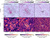 |
Fig. C.1. Polarised Intensity (top row) and its uncertainty maps (bottom row) of the MeerKAT L-band data (left panels), ATCA L/S-band (middle panels) and ATCA C-band (right panels). Total intensity of MeerKAT 1194 MHz (left panels) ATCA 2166 MHz (middle panels) and ATCA 5430 MHz (right panels) contours are overlaid starting at 3σ and increase by a factor of 2 (σ1194 MHz = 30μJy/beam; σ2166 MHz = 15μJy/beam; σ5430 MHz = 11μJy/beam). For each panel, the circular beam appears in the lower left panel. |
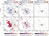 |
Fig. C.2. Foreground-corrected rotation measure (top row) and its uncertainty maps (bottom row) of the MeerKAT L-band data (left panels), ATCA L/S-band (middle panels) and ATCA C-band (right panels). Total intensity of MeerKAT 1194 MHz (left panels) ATCA 2166 MHz (middle panels) and ATCA 5430 MHz (right panels) contours are overlaid starting at 3σ and increase by a factor of 2 (σ1194 MHz = 30μJy/beam; σ2166 MHz = 15μJy/beam; σ5430 MHz = 11μJy/beam). For each panel, the circular beam appears in the lower left panel. |
Appendix D: CRE timescales
This section helps us understand the calculated CRE timescales in Sect. 6.1. The following equations are based on Werhahn et al. (2021) and Basu et al. (2015). For the electron energy, we follow Basu et al. (2015), and write
![Mathematical equation: $$ \begin{aligned} \frac{E}{\mathrm{GeV}} = \biggl [ 7.9\times \biggl (\frac{\nu _{\rm obs}}{\mathrm{GHz}}\biggr )^{1/2} \biggl (\frac{B_\perp }{\upmu \mathrm{G}}\biggr )^{-1/2} \biggr ] \end{aligned} $$](/articles/aa/full_html/2026/04/aa58420-25/aa58420-25-eq20.gif) (D.1)
(D.1)
assuming B⊥ = B, which is the magnetic field strength in the plane of the sky, and νobs the MeerKAT L-band observing frequency. Using the electron energy, we calculate the synchrotron timescale τsyn for CREs emitting at a radio frequency νobs:
 (D.2)
(D.2)
The inverse Compton timescale can be calculated using the radiation field and cosmic microwave background energy density. The cosmic microwave background energy density is UCMB = 4.2 × 10⁻¹³ erg cm−3 (Heesen et al. 2018) and we assume that the radiation energy density is dominated by the magnetic energy density Urad = B2/8π (Heesen et al. 2014). The inverse Compton timescale can be given by
 (D.3)
(D.3)
The bremsstrahlung timescale depends on the average number density of total neutral gas ⟨n⟩ in the ISM, and is given by
 (D.4)
(D.4)
Coulomb interaction losses become typically more significant and effective at lower CRE energies (Petrosian 2001; Ruszkowski & Pfrommer 2023), and are therefore ignored in our analysis. The cooling timescale for a continuous injection of CREs can be calculated by combining all the timescales
 (D.5)
(D.5)
For the escape timescale τesc, we distinguish between two CRE transport processes, namely diffusion and advection. For each process, a characteristic timescale can be calculated to identify the dominant transport mechanism, following (Werhahn et al. 2021). The diffusion timescale of CREs is given by
 (D.6)
(D.6)
where h is the CRE scale height and D is the diffusion coefficient. The timescale for CREs escaping the system via advection is expressed as
 (D.7)
(D.7)
where vesc is the escape velocity. The escape velocity is estimated from the rotation velocity as  (e.g. Heesen et al. 2018).
Furthermore, a spectral analysis is done following Heesen et al. (2014), to estimate the spectral age based on the magnetic field and the frequency of the break νbrk in the spectrum to calculate the time hat has elapsed since freshly accelerated CRe were injected. The spectral age are given by
![Mathematical equation: $$ \begin{aligned} \frac{\tau _{\rm spec}}{\mathrm{Myrs}}= \sqrt{\frac{2.53\times 10^{3} \biggl (\frac{B}{10\upmu \mathrm{G}}\biggr )}{\nu _{\rm brk} \, \biggl [\biggl (\frac{B}{10\upmu \mathrm{G}}\biggr )^2+ \biggl (\frac{B_{\rm CMB}}{10\upmu \mathrm{G}}\biggr )^2\biggr ]^2}} \end{aligned} $$](/articles/aa/full_html/2026/04/aa58420-25/aa58420-25-eq28.gif) (D.8)
(D.8)
where the CMB magnetic field strength is defined as BCMB/μG = 3.2(1 + z)2.
All Tables
Best-fit parameters and the fit statistics of the SED model (ffa1_sfg_sic) for NGC 1487. Uncertainties correspond to 1σ errors.
All Figures
|
Fig. 1. Colour-composite images from the DESI Legacy Imaging Surveys (left panel), HIPASS Hα image (middle panel) and GALEX FUV image (right panel) of NGC 1487 with overlaid MeerKAT radio emission contours starting at 3 σI and increase by a factor of 2 at a central frequency of 1.28 GHz (σI = 4 μJy/beam). The beam of 8.56″ × 7.65″ is shown in the left corner. The scale is calculated using the distance given in Table 1. |
| In the text | |
|
Fig. 2. Left: Total intensity map at 1.28 GHz of NGC 1487 with a noise level σI of 4 μJy/beam observed with MeerKAT. Middle left: Total intensity map at 2.1 GHz of NGC 1487 with a noise level σI of 8 μJy/beam observed with ATCA. Middle right: Total intensity map at 5.5 GHz of NGC 1487 with a noise level σI of 5.5 μJy/beam observed with ATCA. Right: Total intensity map at 9 GHz of NGC 1487 with a noise level σI of 5.5 μJy/beam observed with ATCA. The overlaid contours of the total intensity start at 3 σ and increase by factor of 2. The resolution of the different maps can be taken from Table 3 and is shown in the bottom left corner. |
| In the text | |
|
Fig. 3. Spectral energy distribution of NGC 1487. The plot displays total intensity data with different observations: GLEAM-X data (Ross et al. 2024), RACS-Low data (McConnell et al. 2020), ASKAP EMU main survey (Hopkins et al. 2025), MeerKAT 1.28 GHz data, ATCA L/S-band, C-band, and X-band data presented in this work, and further data from the work of Grundy et al. (2025). We show the best-fit in red with 1σ uncertainty sampled by EMCEE. The blue, orange, and green dotted lines represent the different components of the best-fit model. |
| In the text | |
|
Fig. 4. Inband total spectral index of the MeerKAT L-band (panel a)) and its uncertainty (panel b)) between the frequencies 0.96 and 1.59 GHz overlaid with radio emission at frequency of 1.28 GHz starting at 3σ and increase by a factor of 2 (σ = 9 μJy/beam). The resolution of 12″ is shown in the bottom left corner. Two-point total spectral index (panel c)) and its uncertainty (panel d)) between ATCA L/S-band (2.1 GHz) and C-band (5.5 GHz) overlaid with radio emission at frequency of 2.1 GHz starting at 3σ and increase by a factor of 2 (σ = 11.3 μJy/beam). The resolution of 7″ is shown in the bottom left corner. |
| In the text | |
|
Fig. 5. Region dependent spectral energy distribution, showing total and thermal corrected flux density of MeerKAT L-band, ATCA L/S-, C- and X-band data. The bottom right panel shows the Hα map with the individual regions overlaid in different colours. |
| In the text | |
|
Fig. 6. Total magnetic field strength of NGC 1487 estimated assuming energy equipartition between CR particles and magnetic field. The inner white regions are blank where the equipartition condition is invalid (α > −0.5). The overlaid contours are the total intensity emission at 1.28 GHz. |
| In the text | |
|
Fig. 7. Panel a): Polarised intensity at 1194 MHz with contours starting at 3σPI and increasing by |
| In the text | |
|
Fig. 8. Panel a): Polarised intensity at 2166 MHz with contours starting at 3σPI and increasing by |
| In the text | |
|
Fig. 9. Panel a): Polarised intensity at 5430 MHz with contours starting at 3σPI and increasing by |
| In the text | |
|
Fig. 10. Mean magnetic-field strength maps used as inputs for the CRPropa simulations, shown in face-on (left panel) and edge-on (right panel) projections. The model consists of three logarithmic spiral components centred at APC 1 (0.9 kpc, 0.25 kpc), APC 2 (0.5 kpc, −0.5 kpc), APC 3 (−0.8 kpc, −0.1 kpc) following the star-forming regions identified by Buzzo et al. (2021). A spiral pitch angle of 12° and an X-shaped halo field with an opening angle of 50° are adopted to define the large-scale 3D field structure. |
| In the text | |
|
Fig. 11. Hα map with overlaid magnetic field orientation of the MeerKAT L-band data (in red), ATCA L/S-band data (in pink) and ATCA 5.5 GHz data (in brown). The corresponding resolution is shown in bottom left corner. |
| In the text | |
|
Fig. C.1. Polarised Intensity (top row) and its uncertainty maps (bottom row) of the MeerKAT L-band data (left panels), ATCA L/S-band (middle panels) and ATCA C-band (right panels). Total intensity of MeerKAT 1194 MHz (left panels) ATCA 2166 MHz (middle panels) and ATCA 5430 MHz (right panels) contours are overlaid starting at 3σ and increase by a factor of 2 (σ1194 MHz = 30μJy/beam; σ2166 MHz = 15μJy/beam; σ5430 MHz = 11μJy/beam). For each panel, the circular beam appears in the lower left panel. |
| In the text | |
|
Fig. C.2. Foreground-corrected rotation measure (top row) and its uncertainty maps (bottom row) of the MeerKAT L-band data (left panels), ATCA L/S-band (middle panels) and ATCA C-band (right panels). Total intensity of MeerKAT 1194 MHz (left panels) ATCA 2166 MHz (middle panels) and ATCA 5430 MHz (right panels) contours are overlaid starting at 3σ and increase by a factor of 2 (σ1194 MHz = 30μJy/beam; σ2166 MHz = 15μJy/beam; σ5430 MHz = 11μJy/beam). For each panel, the circular beam appears in the lower left panel. |
| In the text | |
Current usage metrics show cumulative count of Article Views (full-text article views including HTML views, PDF and ePub downloads, according to the available data) and Abstracts Views on Vision4Press platform.
Data correspond to usage on the plateform after 2015. The current usage metrics is available 48-96 hours after online publication and is updated daily on week days.
Initial download of the metrics may take a while.