| Issue |
A&A
Volume 708, April 2026
|
|
|---|---|---|
| Article Number | A184 | |
| Number of page(s) | 13 | |
| Section | Planets, planetary systems, and small bodies | |
| DOI | https://doi.org/10.1051/0004-6361/202558426 | |
| Published online | 09 April 2026 | |
Atmospheric constraints on GJ 1214 b from CRIRES+ and prospects for characterisation with ANDES
1
Instituto de Astrofísica de Andalucía (IAA-CSIC), Glorieta de la Astronomía s/n, Genil, 18008 Granada, Spain
2
Instituto de Astrofísica de Canarias (IAC), 38200 La Laguna, Tenerife, Spain
3
Departamento de Astrofísica, Universidad de La Laguna (ULL), 38206 La Laguna, Tenerife, Spain
4
Department of Astronomy, University of Texas at Austin, 2515 Speedway, Austin, TX 78712, USA
5
Department of Astrophysics, University of Oxford, Denys Wilkinson Building, Keble Road, Oxford OX1 3RH, UK
6
Department of Space Research and Space Technology, Technical University of Denmark, Elektrovej 328, 2800 Kgs. Lyngby, Denmark
7
Space Telescope Science Institute, 3700 San Martin Drive, Baltimore, MD 21218, USA
★ Corresponding authors: This email address is being protected from spambots. You need JavaScript enabled to view it.
; This email address is being protected from spambots. You need JavaScript enabled to view it.
Received:
5
December
2025
Accepted:
2
February
2026
Abstract
Context. Sub-Neptune exoplanets such as GJ 1214 b provide a critical link between terrestrial and giant planets, yet atmospheric characterisation remains challenging due to high-altitude clouds and compressed atmospheres. JWST has recently hinted at molecular signals in GJ 1214 b, and ground-based high-resolution spectroscopy is potentially able to confirm them.
Aims. We aim to constrain the atmospheric composition of GJ 1214 b using all available transits observed with the upgraded CRIRES+ spectrograph on the Very Large Telescope (VLT) by searching for the signatures of water vapour, methane, and carbon dioxide.
Methods. We analysed eight CRIRES+ transit datasets covering the K band (1.90-2.45 μm) at a resolving power of R ≈ 100,000. We used the SysRem algorithm to correct for telluric and stellar contributions and employed the cross-correlation technique with templates from petitRADTRANS to search for H2O, CH4, and CO2. Injection-recovery tests were performed across a grid of metallicities (Z) and cloud-deck pressures (pc) to quantify detection limits. We also generated predictions for ANDES observations using end-to-end simulated datasets with EXoPLORE.
Results. We detect no significant H2O, CH4, or CO2 signatures. Injection-recovery tests show that such non-detections exclude atmospheres with low-altitude clouds and moderate or low metallicities. CH4 yields the tightest empirical limits, with CO2 unexpectedly ruling out intermediate metallicities (∼100× solar) with clouds deeper due to its rapidly rising opacity in compressed high-Z atmospheres. Our constraints are in line with either a high-Z or a high-altitude aerosol layer, in agreement with recent JWST inferences.
Conclusions. The combined analysis of eight CRIRES+ datasets provides the most stringent high-resolution constraints on the atmospheric properties of GJ 1214 b to date. Planetary signals are likely buried below our current detection threshold, preventing confirmation of recent JWST-reported molecular hints. Simulations of a single transit observed with ANDES on the ELT predict modest improvements for H2O, a substantially expanded detectable region for CH4, and the strongest gains for CO2, making the latter a particularly effective tracer for characterising high-metallicity atmospheres in sub-Neptunes.
Key words: methods: observational / methods: statistical / techniques: spectroscopic / planets and satellites: atmospheres / planets and satellites: individual: GJ 1214 b
© The Authors 2026
 Open Access article, published by EDP Sciences, under the terms of the Creative Commons Attribution License (https://creativecommons.org/licenses/by/4.0), which permits unrestricted use, distribution, and reproduction in any medium, provided the original work is properly cited.
This article is published in open access under the Subscribe to Open model. This email address is being protected from spambots. You need JavaScript enabled to view it. to support open access publication.
1 Introduction
Sub-Neptune-size planets are now recognised as one of the most common outcomes of planet formation, dominating the radius distribution between roughly 1.5 and 4 R⊙ (Fulton et al. 2017; Fulton & Petigura 2018). Despite their relative similar sizes, these planets seem to span a wide diversity of interior structures: some are consistent with high-density, rocky, or water-rich compositions, whereas others appear to host low-density H/He envelopes (e.g. Luque & Pallé 2022; Parc et al. 2024; Venturini et al. 2024; Lichtenberg et al. 2025). In principle, sub-Neptunes with H/He envelopes should imprint prominent spectroscopic features during the exoplanet’s primary transit. However, a decade of observations has repeatedly yielded featureless or strongly muted transmission spectra for many of these worlds with space telescopes at low-resolution (e.g. Kreidberg et al. 2014; Libby-Roberts et al. 2022; Lustig-Yaeger et al. 2023; Kahle et al. 2025; Bennett et al. 2025b,a) and ground-based, high-resolution instrumentation (e.g. Spyratos et al. 2021; Jiang et al. 2023; Dash et al. 2024; Grasser et al. 2024; Parker et al. 2025). GJ 1214 b (Charbonneau et al. 2009), a benchmark sub-Neptune subjected to intensive atmospheric scrutiny (e.g. Bean et al. 2010; Miller-Ricci & Fortney 2010; Kempton et al. 2011; Morley et al. 2013; Kreidberg et al. 2014; Orell-Miquel et al. 2022; Kempton et al. 2023; Nixon et al. 2024; Schlawin et al. 2024; Ohno et al. 2025), is a prime example of this phenomenon, after its featureless spectrum became emblematic of the difficulties faced in characterising this planetary population (Bean et al. 2010; Kreidberg et al. 2014).
Multiple mechanisms have been proposed to explain these muted spectra. Extinction by high-altitude aerosols can obscure molecular features (Morley et al. 2013; Kreidberg et al. 2014), while extremely metal-enriched atmospheres would raise the mean molecular weight high enough to suppress their amplitude (e.g. Kempton et al. 2023). Due to the frequency of featureless spectra found, both processes could be widespread across the sub-Neptune population (Lee et al. 2025; Welbanks et al. 2025). The recent arrival of the James Webb Space Telescope (JWST) has dramatically improved this landscape, as molecular detections (including water vapour, carbon dioxide, or methane) have been confirmed in several sub-Neptunes (Benneke et al. 2024; Holmberg & Madhusudhan 2024; Schmidt et al. 2025), allowing robust constraints on atmospheric metallicities and cloud properties. However, a significant part of the observations are still limited by apparent aerosol extinction, as is the case for GJ 1214 b (Kempton et al. 2023; Schlawin et al. 2024; Ohno et al. 2025), L98-59c (Scarsdale et al. 2024), or GJ3090b (Ahrer et al. 2025).
Observations using high-resolution spectroscopy (HRS; R ≳ 40 000) emerged as potentially one of the most effective approaches for characterising aerosol-rich exoplanet atmospheres (Hood et al. 2020). Applying the well-known crosscorrelation (CC) technique to these data, we are, in principle, capable of probing thin atmospheric layers above the high clouds of sub-Neptunes (Birkby 2018; Snellen 2025). This is because HRS data allow us to resolve the core and wings of spectral lines, in contrast to low-resolution studies. This makes it an ideal technique to attempt detections in hazy exo-atmospheres, where only line-cores may protrude above the continua provided by a clouddeck (e.g. Pino et al. 2018a,b; Sánchez-López et al. 2020; Gao et al. 2021). Indeed, HRS characterisation of exoplanet atmospheres has allowed the detection of single species (Charbonneau et al. 2002; Snellen et al. 2008, 2010; Brogi et al. 2012; Birkby et al. 2013; de Kok et al. 2013; Lockwood et al. 2014; Casasayas-Barris et al. 2021; Stangret et al. 2022) and multiple molecules in the past (Hawker et al. 2018; Cabot et al. 2019; Kesseli et al. 2020; Giacobbe et al. 2021; Cont et al. 2021; Sánchez-López et al. 2022a) at layers that can typically span pressures below 1 mbar (higher altitudes than this pressure level).
A particularly valuable tracer of atmospheric escape in closein, low-density exoplanets is the metastable helium triplet at 1083 nm, observable with high- and low-resolution spectroscopy (Seager & Deming 2010; Oklopcic & Hirata 2018). This feature probes the structure of the thermosphere and has revealed extended, escaping atmospheres in several sub-Neptunes and warm Neptunes (Spake et al. 2018; Allart et al. 2018; Nortmann et al. 2018). GJ 1214b (Charbonneau et al. 2009) is a warm subNeptune benchmark (2.7 R⊕, 8.1 M⊙) orbiting an M4.5 dwarf every 1.58 days and has been the focus of extensive observational campaigns aimed at constraining its atmospheric composition. Several high-resolution searches for He I have been conducted at 1083 nm and can only place upper limits (e.g. Crossfield et al. 2019; Petit Dit de la Roche et al. 2020; Kasper et al. 2020; Orell-Miquel et al. 2022; Spake et al. 2022) or a tentative detection (Orell-Miquel et al. 2022) on the planetary absorption. None have yielded robust conclusive detection.
GJ 1214 is not considered a highly active M dwarf in terms of strong flares or chromospheric emission, but long-term photometric monitoring and transit analyses have revealed the presence of spots and active regions on its surface (Berta et al. 2011; Carter et al. 2011; Narita et al. 2013; Nascimbeni et al. 2015; Rackham et al. 2017; Mallonn et al. 2018). Photospheric heterogeneity can influence transit depths and potentially introduce epoch-to-epoch variations in transmission spectroscopy. Nevertheless, currently there is no evidence that such moderate activity levels significantly modulate the He I 1083 nm signal.
A powerful instrument for HRS in transmission is the upgraded Cryogenic high-resolution InfraRed Echelle Spectrograph (CRIRES+; Kaeufl et al. 2004; Follert et al. 2014; Dorn et al. 2014). Due to its high spectral resolution of R≈ 85 000100000, CRIRES+ is in principle sensitive enough to detect the strong spectral features that form at low pressures above potential clouds, depending on the actual conditions in the exoplanet. In this paper, we compiled all available datasets observed with CRIRES+ for GJ 1214 b (eight transits in total) to explore its atmospheric composition. In Sect. 2, we describe these observations. The methods used for the analysis of the spectral data are based on the well-known cross-correlation technique, which is detailed in Sect. 3. We present and discuss our results in Sect. 4, including prospects for atmospheric characterisation of GJ 1214 b with the next generation of telescopes and instruments such as ArmazoNes high Dispersion Echelle Spectrograph (ANDES; Marconi et al. 2022; Palle et al. 2025), and we outline our main conclusions in Sect. 5.
Stellar and planet parameters of the GJ 1214 system.
2 Observations
We analysed eight datasets from the public ESO archive observed with the CRIRES+ spectrograph, installed at the 8.2m Unit Telescope 3 of the ESO’s Very Large Telescope (VLT) at Cerro Paranal. The observations were carried out between 12 March 2022 and 6 August 2024 in the K band, using the K2148 wavelength setting. This setting covers the 1.90-2.45 μm range over eight spectral orders, at a resolving power of R ≈ 100000. In Table 1 we summarise the stellar and planetary parameters used in this study. The eight analysed datasets cover the pre, during, and post-transit phases of GJ 1214b, from φ = −0.0114 to φ = 0.0114; (see Fig. 1). A ninth (17 August 2024) was available, but its low S/N and poor coverage of the transit event made it unsuitable for inclusion in our analysis. The S/N for all eight nights ranges from ∼55 to ∼120. All datasets show relative humidity below 20%, except for the night of 12 March 2022, when it was about 30%. Further details on the observation conditions for this night are provided in Table 2.
The CRIRES+ raw data for GJ 1214 b were retrieved from the ESO Archive1 and reduced using the standard CR2RES pipeline routines (version 1.4.4) using the ESO Recipe Execution Tool (EsoRex, version 3.13.8). This pipeline includes dark calibration (not used during nodding subtraction), bad-pixel masking, flat calibration, wavelength calibration using a combination of the Fabry-Pérot etalon and uranium-neon lamp, and 1D spectral extraction. The observations consisted of 7.5 nodding cycles, following the ‘A1,2,3, B1,2,3, B4,5,6, A4,5,6,’ nodding pattern. In order to perform nodding subtraction, we regrouped the nodding pairs as A1B1, A2B2, ... A6B6. The spectra were extracted using the optimal extraction algorithm, with a fixed extraction height of 20 pixels (∼8 times the median full width at half maximum (FWHM) of the point spread function along the slit) and no-light rows subtracted. In addition, we discarded the bluest order (order 29; 1.90-1.95 μm) due to strong telluric absorption. The observations were conducted in adaptive optic mode and, due to the seeing conditions (∼0.65″), the slit was not evenly illuminated in the dispersion direction during the observations. Although this might cause a slight spectral shift between the positions A and B (as described in the CR2RES user manual2), no significant spectral shift above the velocity resolution of the instrument (1 kms−1) was detected when cross-correlating the A and B spectra.
GJ 1214’s CRIRES+ analysed spectroscopic observations.
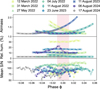 |
Fig. 1 volution of the airmass, relative humidity, and mean S/N per spectrum. The pink-shaded area marks the in-transit times. Nodding A spectra are represented with empty symbols and Nodding B spectra with filled symbols. |
3 Methods
Before performing any further operations on the data, we took into account the differences in the pixel-wavelength solution between the nodding A and B position spectra by interpolating the pixel-wavelength solution from nodding position B to position A. In addition, we removed the edges of each spectral order (the first and last 100 pixels), as they show increased systematics. With all of the spectra in a common wavelength solution (that of A spectra), we proceeded with the usual steps for our purpose with high-resolution spectra.
3.1 Normalisation, outliers, and masking
Ground-based observations of exo-atmospheres suffer from an inherent disadvantage stemming from the varying conditions of Earth’s atmosphere (e.g. seeing and precipitable water vapour variability). Some spectra presented anomalous spectral behaviour, with unexpected peaks or valleys in the recorded counts, potentially caused by transient high-altitude clouds in Earth’s atmosphere. Other spectra displayed a sharp decrease in the mean S/N compared to those taken immediately before and after. In these cases, we discarded the spectra from the analysis to avoid hindering the telluric correction (see discarded spectra listed in Table 2). In addition, variations during observations induce a fluctuating baseline in the spectra (Fig. 2B). Thus, to provide a common continuum to all spectra, we performed an order-by-order normalisation by fitting a third-degree polynomial to the pseudo-continuum (Fig. 2C).
Next, following the approach used by Kesseli & Snellen (2021), we removed any possible contamination coming from cosmic rays by applying a 3σ-clipping procedure where we flagged values that significantly deviate from the mean of the pixel’s time series. We acknowledge that this procedure’s threshold is conservative compared to others (e.g. 5σ-clipping). However, given the high S/N of our datasets and the exposure times used, the distribution of the normalized flux at each pixel is expected to be well approximated by a Gaussian distribution. Moreover, previous studies have successfully applied this method using a comparable number of spectra per dataset (Kesseli & Snellen 2021; Sánchez-López et al. 2022b; Casasayas-Barris et al. 2022; Peláez-Torres et al. 2025). Flagged values were corrected by interpolating them over their nearest neighbours in wavelength. The most opaque windows of Earth’s atmospheric transmittance (telluric) were masked whenever 85% of the normalised flux was absorbed and also interpolated over their nearest neighbours. A safety window of 5 pixels was added to each flagged pixel to further limit the potential contamination of strong telluric-line wings.
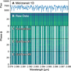 |
Fig. 2 Steps of the data preparation applied to a representative spectral region of the dataset obtained on the night of 31 March 2022. The vertical axis in panel A represents flux in arbitrary units, while in all other panels it represents time, expressed as the planet’s orbital phase. Panel A: original spectrum observed at mid-transit, where telluric absorption lines from H2O can be identified. Panel B: original spectral matrix extracted using CR2RES, where major S/N differences between spectra (horizontal stripes) and prominent telluric H2O absorption (vertical stripes) can be identified. Panel C: normalised and masked spectra, where opaque telluric windows are excluded (white stripes). Panel D: residual spectra after one SysRem pass, where telluric residuals can be observed. Panel E: residual spectra after nine SysRem passes, where most of the telluric contribution has been removed. Nodding position effects were corrected in all panels by interpolating the pixelwavelength solution from nodding position B to position A. |
3.2 Telluric and stellar correction
Even after masking the most opaque windows, telluric and stellar features within the spectra are several orders of magnitude stronger than the Doppler-shifted excess absorption from the planetary atmosphere. In order to disentangle the exo-atmospheric signal, we used SysRem (Tamuz et al. 2005; Mazeh et al. 2007), an iterative principal component analysis algorithm that accounts for unequal uncertainties for each data point. SysRem has been successfully applied in similar studies in the past to reveal signatures in the atmosphere of several exoplanets (de Kok et al. 2013; Birkby et al. 2013, 2017; Sánchez-López et al. 2019; Nugroho et al. 2020; Cont et al. 2022; Maguire et al. 2024; Nortmann et al. 2025).
Contamination at different levels affect each spectral order depending on the spectral shape of the telluric transmittance. If a single global number of SysRem passes is adopted, there is a risk of over- or under-correcting for telluric features, which could either erase the planetary signal or leave residual contamination that hinders detection. This results in the number of required SysRem passes being order-dependent, and a criterion needs to be set to determine it. This is a difficult step that can lead to unintended biases and even spurious planet-like signals, depending on the criterion employed (see, e.g. Cabot et al. 2019; Cheverall et al. 2023). We therefore determined the appropriate number of SysRem passes individually for each spectral order following a similar approach to Herman et al. (2020, 2022); Deibert et al. (2021); Rafi et al. (2024), and Parker et al. (2025). We studied the variance of the residual spectral matrices after applying SysRem and halted the algorithm when the difference in standard deviation between two consecutive passes (Δσ) was below a given threshold (1%) and started to plateau. In practice, this method helps recognise when ∆σ plateaus for each spectral order, indicating that the major spectral variations have been removed and no further passes are required. This should also preserve signals close to the noise level, such as the exo-atmospheric absorption, while also being a model-independent approach, in contrast to optimisation based on injection-recovery techniques. The ∆σ metric is thus defined as
 (1)
(1)
where (i−1)σ and (i)σ are the standard deviations of the residuals in spectral order before and after the i-th pass of SysRem, respectively (Parker et al. 2025).
In the defined metric, a plateau is typically reached between five to seven SysRem passes for the CRIRES+ datasets, depending on the spectral order, as illustrated in Fig. A.1. This indicates the number of SysRem passes adopted for each spectral order. During the first SysRem pass, telluric and stellar features still remain (panel D of Fig. 2), suggesting the need for further cleaning. For intermediate to final passes, the exo-atmospheric signal, if present, is expected to be buried in the noise (Fig. 2E).
3.3 Model atmospheres
We modelled the exo-atmospheric transmission spectra of GJ 1214b using petitRADTRANS3 (pRT), a Python-based package for calculating the transmission and emission spectra of exoplanets through radiative transfer (Mollière et al. 2019). We assumed H2-He dominated atmospheres where Rayleigh scattering and collision-induced absorption are included (Figueira et al. 2009; Nettelmann et al. 2010). The same preparation steps performed on the real data were applied to the models to ensure that the same distortions are introduced.
We included in the pRT models the absorption of the most relevant spectroscopically active species in the covered nearinfrared (NIR) range, that is, H2O, CO2, CO, NH3, H2S, using the line lists presented by Rothman et al. (2010) and CH4 by Hargreaves et al. (2020). Specifically, in Sect. 4 we search for H2O, CO2, and CH4. Model transmission spectra were generated on a 2D-grid spanning the pressure level of a potential cloud deck (pc) and the metallicity of the atmosphere (Z). This latter step was facilitated by the algorithm easyCHEM4 (Lei & Mollière 2025), which provides the mass fractions of the atmospheric compounds and the mean molecular weight (thus, the atmospheric scale height) as a function of the metallicity, for an isothermal P-T profile at the equilibrium temperature of the planet (see Table 1). Throughout this work, we fixed the atmospheric carbon-to-oxygen ratio to a solar value of 0.55 (Asplund et al. 2009), which agrees well (within uncertainties) with the JWST-derived values reported in Ohno et al. (2025). Our pc grid spanned from 0.1 mbar to 1 bar, while the Z grid covered from 1× solar to 1000× solar metallicity. Grid values were evenly spaced on a logarithmic scale, resulting in a total of 100 templates per molecule. Fig. A.3 illustrates the variations of the transit depth in the models due to changes in both pc and Z in the wavelength range covered by the K2148 setting of CRIRES+. For each Z-pc pair, we compute two types of transmission models: (i) those that include all spectroscopically active species in the K2148 setting of CRIRES+, which will be injected into the data prior to preparation for detectability studies in Sect. 4, and (ii) models tht include only a specific species’ opacity, which will be used as the cross-correlation (CCF) template. We note that, in the latter case, we still consider all species from easyCHEM to assess the atmospheric composition and the scale height appropriately. Further discussion is provided in Sect. 4.
3.4 Cross-correlation technique
Any potential atmospheric lines from GJ 1214 b remain buried below the noise level in the residual spectra. Using the crosscorrelation technique (Snellen et al. 2010), it is possible to co-add the contribution from potentially hundreds of these lines in the form of a CCF peak (e.g. Birkby 2018; Snellen 2025). We performed the cross-correlation between the residual matrices obtained in the previous steps Rij (where i denotes each spectrum and j the wavelength dimension) and the transmission models (templates) mj calculated using pRT. In order to explore a wide range of velocities with respect to the Earth, we used linear interpolation to Doppler-shift the templates in a range of velocities v from −325 to +325 km s−1 with respect to the Earth. We used 1 km s−1 intervals, as set by the average velocity step size between the instrument’s pixels. Given the CCF- and S/N-based metric used in this work, we do not expect any oversampling even in regions where the pixel velocity spacing becomes larger than the adopted step-size (1 km s−1) (Sánchez-López & Millán 2025). The CCFs were obtained individually for each spectrum, i, forming a cross-correlation matrix, CCF(v, i), as follows
 (2)
(2)
where  are the propagated uncertainties of the data and the summations loop over wavelength (λ) and spectral order j, so as to co-add the potential information contained in our full spectral coverage. The resulting total CCF(v, i) in the Earth’s rest frame is illustrated in Fig. 3, together with the trace where GJ 1214b would be expected to appear during the transit (i.e. between the horizontal dash-dotted red lines) along the planetary radial velocity with respect to the Earth, vp. To describe the orbit of GJ 1214 b, we use the definition of vp as follows
 (3)
(3)
where φ is the orbital phase, vbary the barycentric velocity due to Earth’s motion around the Solar System’s barycentre, vsys the systemic velocity of the star-planet system, and Kp the radial velocity semi-amplitude of the planet, defined as
 (4)
(4)
where a is the orbital parameters (the semi-major axis), Porb the orbital period, e the eccentricity, and i the inclination. It is at this point that we visually inspected the cross-correlation matrices in the Earth’s rest-frame for all spectral orders and for each night separately (see Fig. A.2). We discarded from the analysis one spectral order with uncorrected systematics (see Table 2).
Next, we co-added all in-transit CCFs along the time axis (i.e. sum Eq. (2) over i) to maximise any potential signal. To do this, we first Doppler-shifted CCF(v, i) to the exoplanet’s restframe by using Eq. (3), assuming Kp as unknown and using a range of values from −300 to 300 km s−1 in steps of 1 km s−1. Thereby, an absorption with a planetary origin should only appear around the expected Kp of GJ 1214 b (i.e. the exoplanet’s rest frame) in the form of a CCF peak.
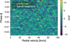 |
Fig. 3 Cross-correlation analysis of potential H2O signals in the transmission spectrum of GJ 1214 b observed with CRIRES+ in the nearinfrared. The method is illustrated for the night of 31 March 2022. We show the cross-correlation matrix in the Earth’s rest frame as a function of the velocity Doppler shifts applied to the template (horizontal axis) and the planet’s orbital phase (vertical axis). The results were obtained by using a template with 10× solar metallicity and a 10 mbar cloud deck. All useful spectral orders were combined. White lines mark the transit start and end times, while the yellow lines indicate the expected exoplanet velocities with respect to Earth. |
3.5 Assessment of potential signals
Following common signal significance evaluation approaches, we computed a S/N map as a function of the exoplanet restframe velocity and Kp (top panel of Fig. 4; Birkby et al. 2017; Brogi et al. 2018; Alonso-Floriano et al. 2019; Sánchez-López et al. 2019; Nugroho et al. 2021; Cont et al. 2022, 2024). For each Kp we divided each CCF point by the CCF’s standard deviation, excluding a ±20 km/s window around it. The division ensured that we avoided inflating the standard deviation by including possible CCF-peak wings. The potential signals are thus evaluated on a common Kp-vrest map, as shown in the top panel of Fig. 4. In this case, the map does not reveal any significant signals (e.g. at S/N> 4) in the expected Kp (bottom panel of Fig. 4). All the observed patterns could be well explained by noise fluctuations or weak telluric residuals. This then leads to a non-detection of water vapour in GJ 1214 b when using this particular CRIRES+ dataset observed on 31 March 2022. The same methods are subsequently applied to all transit datasets (see Fig. A.4).
To enhance the recovery of a potential planetary signal, we combined the information from each observed night by creating a merged CCF map. In this process, we sorted the frames from all datasets along the time axis according to their corresponding orbital phases following the approach of Cont et al. (2022, 2025). The respective  of each spectrum was considered at the time of Doppler-shifting the CCF matrix from the Earth’s rest-frame to the planet’s. This procedure thus yielded a single CCF map, which incorporates all the data from the different nights and is used to compute the Kp-vrest and S/N maps in the same way as for a single-night dataset.
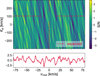 |
Fig. 4 Significance analysis of potential H2O signals, illustrated for the night of 31 March 2022. Top panel: S/N map as a function of radial velocity in the exoplanet’s rest frame (vrest, horizontal axis) and the projected orbital velocity semi-amplitude, Kp (vertical axis). Horizontal lines mark the expected Kp, and vertical lines show the zero rest-frame velocity. Bottom panel: 1D cross-correlation function at the expected Kp (97.1 kms−1)of GJ 1214b. |
4 Results and discussion
When performing direct cross-correlation of the residual data after SysRem with H2O, CH4, and CO2 templates (pc = 10 mbar, Z = 10 × solar) for the eight transit observations of GJ 1214 b with CRIRES+ we were not able to detect either water vapour, methane, or carbon dioxide in the atmosphere of this planet (see Fig. 5). That is, all signals on the map have significances around or below the S/N = 3 level, hence being consistent with noise. This is in agreement with most of the previous observations of this exoplanet's atmosphere, which is historically reported to be cloudy, thus presenting muted spectral features. Unfortunately, this also means we were unable to confirm at high resolution and using transit spectra any of the recently reported hints of molecular features from JWST data (Kempton et al. 2023; Schlawin et al. 2024; Ohno et al. 2025).
As it is a standard approach, the lack of molecular signatures in our K band spectra motivated the exploration of the Z and pc parameter spaces. To date, different methods have been used to construct the Z-pc grid: (1) a direct S/N metric where the grid is built using the pure S/N value (Grasser et al. 2024; Peláez-Torres et al. 2025); (2) an alternative analysis based on Δσ in which the S/N value used in the grid comes from a likelihood framework (Log(L)) (Parker et al. 2025); and (3) a Log(L) grid in which the fit quality of each tested model is compared against the best fitting model (Lafarga et al. 2023; Dash et al. 2024). In this study, we used the method (1). Thus, using the previously generated set of models (see Sect. 3.3), we performed injection-recovery tests to assess the detectability of different atmospheric properties in the planet with our combined observations (direct S/N metric). The atmospheres of the injected model hence include a full mean-molecular weight and mass fraction assessment by easyCHEM, plus the opacity contributions from H2, He, H2O, CO2, CO, CH4, NH3, and H2S in the transmission spectrum calculation from petitRADTRANS (Fig. 6). Regarding the CCF template, it only includes one opacity source, that of the species to be recovered (see Sect. 3). Using only the opacity of one molecular absorber (besides H2) in the template reproduces the usual approach of CCF studies, where single-species templates are cross-correlated with exo-atmospheric data containing a wealth of spectral contributions, hence avoiding overly optimistic detectability estimations (see discussion in Parker et al. 2025). The resulting detectability maps are shown in Fig. 7 for the cases of H2O, CH4, and CO2.
Methane explorations placed the strongest upper limits (S/N = 5 contour), discarding atmospheres with pc ≲ 10-4 bar for metallicities lower than 50× solar. The parameter space discarded by H2O analyses is fully contained in the CH4 -derived results. Both contours are in good agreement in their higher metallicity boundary (50× solar), but H2O places a weaker restriction in the potential cloud deck location at all metallic-ities, and especially at solar values. This occurs because CH4 lines in the K band setting used in these observations contaminate the H2O spectrum more strongly than the reverse, even though individual water vapour lines are intrinsically stronger.
Interestingly, CO2 explorations yielded a surprisingly strong constraint (also a S/N = 5 contour) that discards atmospheres for metallicities in the range 40 < Z/Z⊙ < 200 and clouds at altitudes lower than the 1 mbar level. In this intermediate- to high-metallicity regime and for the fixed C/O ratio of 0.55 adopted in our chemical grid, the CO2 abundance increases with greater availability of carbon and oxygen atoms in the atmospheric reservoir. Consequently, the growth in CO2 line opacity seems to outpace the loss of signal due to the reduced scale height at high metallicities. This balance, also suggested by Parker et al. (2025), opens a window for characterising more compressed atmospheres in the K band for similar targets.
Overall, these results agree very well with the traditional observation-derived view of this exoplanet (e.g. Bean et al. 2010; Berta et al. 2012; Kreidberg et al. 2014), which found that its atmosphere is covered by clouds that mute potential spectral features originating at altitudes below the cloud top deck. Our most restrictive H2 O-derived upper limits agree very well with the best-fit scenario discussed in Kempton et al. (2023), including high-altitude aerosols, a high-metallicity atmosphere, or both scenarios simultaneously.
It is also common to perform Bayesian retrievals to explore the parameter space we have discussed, since these represent powerful frameworks for assessing the properties of exoplanet atmospheres (Gibson et al. 2020; Brogi & Line 2019; Blain et al. 2024; Lesjak et al. 2025; Peláez-Torres et al. 2025). However, we did not consider that a Bayesian retrieval would provide additional meaningful constraints on the atmosphere of GJ 1214b with our current datasets.
In Peláez-Torres et al. (2025), a similar analysis combining high-resolution CARMENES and CRIRES+ observations of GJ 436 b showed that Bayesian retrievals confirmed nondetection of molecular species through cross-correlation analyses. In that study, the retrievals and injection-recovery experiments were found to be mutually consistent, with the retrieval posterior fully contained within the non-detectable region of parameter space according to CCF results. Comparable conclusions can be extracted from H2O studies of KELT-11 b and WASP-69b in Lesjak et al. (2025). Following the same rationale, we conclude that a Bayesian retrieval applied to our GJ 1214 b datasets would not yield additional constraints beyond injection-recovery tests.
Next-generation facilities like ANDES at the ELT are poised to revolutionise the field of exoplanet characterisation. To assess the capabilities of ANDES to probe the atmosphere of GJ 1214 b, we used EXoPLORE, a comprehensive, end-to-end simulator of high-resolution observations, which is based on the techniques presented in Blain et al. (2024) and has been recently used for this aim in Peláez-Torres et al. (2025). EXoPLORE is designed to produce realistic in silico time-series spectra, incorporating ANDES’ wavelength coverage for the K band (planned) and S/N based on ANDES exposure time calculator (Sanna et al. 2024) assuming exposure times of 30 s, a resolving power of R = 100000, and telluric evolution as a function of the airmass. It is important to note that the current version of the simulator does not yet incorporate additional sources of correlated noise or water vapour variability, which can greatly hinder telluric correction. These remain active areas of development, and consequently, the results presented here should be considered as optimistic approaches to the real performance of ANDES. Using EXoPLORE, we investigated the same grids in atmospheric metallicity and cloud-top pressure as in previous sections. For each combination, a complete simulated dataset was generated incorporating four main spectral contributions:
The Earth’s atmospheric transmittance as a function of the airmass from ESO’s Skycalc Tool (Noll et al. 2012; Jones et al. 2013);
The exoplanet signal including H2, He, H2O, CO2, CH4, NH3, and H2S, Doppler- shifted at each synthetic exposure following Eq. (3) and scaled by the transit’s light curve computed with the BATMAN package (Kreidberg 2015), assuming a uniform stellar disc and the system parameters of GJ 1214 b listed in Table 1 and from Mahajan et al. (2024);
The host star, with a PHOENIX stellar template (Husser et al. 2013) with Teff = 3000 K, log(g) = 5.0, and [Fe/H] = 0.0, consistent with the properties of GJ 12145.
Random noise for each spectral point and exposure, generated using Python’s functions np.random.default_rng() and rng.normal(). Using the ETC, the standard deviation for the Gaussian distribution was computed as
 .
.
Next, we analysed the simulated dataset following the techniques we presented in Sect. 3, and the signal recovered at the expected exoplanet Kp and vrest was stored for the particular (Z/Z⊙, pc) tuple. We note that, in agreement with our injection recovery tests (Fig. 7), the CCF templates were computed using the easyCHEM-derived mean-molecular weight, including all equilibrium species, but using only single-species’ opacity in petitRADTRANS. It is instructive to place these simulations in the context of existing VLT∕CRIRES+ observations. The number of detected photons scales as Nγ ∝ D2 Texp, where D is the telescope diameter and Texp the exposure time. Using the exposure times adopted here (30 s for the ELT and 240 s for the VLT), the photon ratio per exposure (i.e. the collective power comparison) can be roughly estimated as
 (5)
(5)
Thus, a single 30 s ANDES exposure collects nearly three times more photons than a 240 s CRIRES+ frame. When comparing whole transits, the scaling simplifies if we assume similar overheads: ANDES observes one transit with exposure times eight times shorter, while we combined eight CRIRES+ transit datasets that have, except for one night (27 May 2022, Table 2), exposures eight times longer. These two factors cancel each other out, and the total photon ratio for an entire transit remains the same factor of ∼2.8. In the photon-limited regime, the S/N scales as  , so a single ANDES transit is expected to achieve a higher S/N per exposure by a factor of
 (6)
(6)
That is roughly a 70% improvement in line-contrast S/N compared to the full eight-transit CRIRES+ dataset. This estimate assumes comparable throughputs for ANDES and CRIRES+ and therefore must be understood as a conservative photon-limited comparison. It is important to note that the injection-recovery analysis used for CRIRES+ data differs in important ways from the idealised ANDES simulations presented here. In particular, the injected planetary signal to obtain the results of Fig. 7 is not scaled by the transit light curve during ingress and egress, artificially strengthening the recovered signal. Conversely, the VLT data contain real telluric and instrumental residuals that are not fully captured in our simulated spectra, although we did not observe significant telluric residuals in the included spectral orders across nights. These differences should be taken into account when comparing in silico with empirical results.
The predicted detectability maps obtained with ANDES, for a single transit observation of GJ 1214 b and search for water vapour, methane, and carbon dioxide, are shown in Fig. 8. A natural way to interpret the ANDES simulations is to compare them directly with the constraints obtained from the CRIRES+ injection-recovery tests from Fig. 7. In all cases, the in silico S/N maps for a single ANDES transit reproduce the overall structure of the empirically derived detectability contours, while extending the excluded region of parameter space in a way that reflects the underlying line strengths and chemical behaviour of each molecule.
For H2O, the empirical and in silico S/N = 5 contours (SN5) are remarkably similar across the explored Z-pc plane, with only a modest shift towards slightly higher metallicities and somewhat deeper cloud decks at the high-Z end. This is consistent with the fact that H2O does not dominate the opacity in the K band at GJ 1214 b’s equilibrium temperature. That is, H2O lines are strong, but they are partially blended with CH4 and other species, and the significant overlap with these other near-infrared absorbers shifts the detectability of H2O from a photon-limited to a signal-limited regime, and hence its measurement does not benefit much from the increased collecting area of the ELT. In other words, the small difference between the empirical and in silico contours indicates that we are already approaching a regime where H2O detectability is limited by intrinsic atmospheric effects, namely the mixture of overlapping opacities and the reduced scale height at high metallicity, which together weaken the H2O lines to undetectable levels. This contrasts with the photon-limited regime, where detectability could still be improved by collecting more photons.
Methane inferences behave more in line with a priori expectations of its line density in this wavelength range. In the CH4 detectability map, the in silico SN5 contour for a single ANDES transit excludes a significantly larger region of parameter space than the empirical CRIRES+, particularly at high metallicities and for cloud decks deeper than 0.1 mbar. In silico, a S/N = 14 threshold is reached compared to the maximum S/N ≈ 10 of the empirical case, which is consistent with the expectation that ANDES should deliver an overall gain (photon-limited) in the order of ∼1.7 in line-contrast S/N relative to the eight-transit CRIRES+ set. This in general reflects the fact that CH4 provides the densest and intrinsically strongest set of lines for CCF in the K band for a cool metal-rich atmosphere like that expected for GJ1214b.
The behaviour of CO2 further emphasises the role of chemistry in shaping the detectability we observed in Fig. 7. In the CO2 maps, the empirical SN5 contour from CRIRES+ data limits the parameter space to a region of intermediate metallic-ities around 100× solar and relatively low cloud-top pressures of pc < 1 mbar. The in silico ANDES SN5 contour presents a similar morphology, modestly pushing upwards the pc boundary for Z/Z⊙ = 100, while significantly expanding towards a broader range of metallicities, beyond 1000× solar for lower-altitude clouds. As discussed for empirical injection-recovery tests, this suggests that the steep increase in CO2 abundance with metallic-ity translates into a line opacity in the K band that rises strongly enough to compensate for the high-Z reduction in the features’ amplitude. In that situation, the CO2 signal would remain effectively photon-limited over a wider metallicity range, and hence increasing the collecting area directly impacts the detectability in compressed atmospheres with relatively deep clouds. Therefore, the ANDES predictions strengthen, rather than qualitatively change, the picture already suggested by the CRIRES+ analysis, deeming CO2 an especially powerful tracer of high-Z regimes in GJ 1214 b, and similar sub-Neptunes, within the K band.
 |
Fig. 5 Cross-correlation maps in S/N units for potential atmospheric signals as a function of vrest and Kp for the primary expected absorbing species in the atmosphere of GJ 1214 b. We explored water vapour (left), methane (middle), and carbon dioxide (right). Horizontal and vertical red lines indicate the expected Kp and vrest. These example maps were derived using a 10× solar metallicity template with a cloud deck at 10 mbar. No molecular signals were detected in our cross-correlation analyses. |
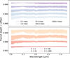 |
Fig. 6 Transit depth of the main absorbers (H2, He, H2O, CO2, CO, CH4, NH3, and H2S) for GJ 1214 b in the analysed K band range as a function of cloud deck pressure level (top panel, fixed metallicity of 10× solar) and atmospheric metallicity (bottom panel, clear atmosphere) as multiples of solar. For clarity, an offset of 0.002 in transit depth was applied to the transmission models in both panels. |
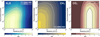 |
Fig. 7 Detectability maps obtained from injection-recovery tests, showing upper limits on the abundances of the main near-infrared strongest absorbers in the atmosphere of G 1214 b. Specifically, we investigate H2O (left panel), CH4 (middle panel), and CO2 (right panel) across a range of metallicities and cloud deck altitudes. Dashed lines indicate the S/N = 5 contours for H2O, CH4, and CO2, as obtained from CRIRES+ (white, eight transits combined). The lower S/N of CO2 recoveries stems from its weaker and fewer lines in the K band, compared to the other infrared absorbers. Red dotted lines indicate the upper limits derived in Kempton et al. (2023) from day and nightside evidences of H2O observed with JWST, in the best-fitting case of reflective clouds and high metallicity. |
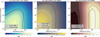 |
Fig. 8 Simulated detectability maps of GJ 1214 b computed with EXoPLORE, assuming a single-transit observation with ANDES on the upcoming ELT. We compute the case of H2O (left), CH4 (middle), and CO2 (right). The white (only for CH4) and red contours indicate recovered S/N levels of 10 and 5 in ANDES in silico data, respectively. For comparison purposes, we also include the S/N = 5 curves (black) obtained from the empirical data analysed in this work (Fig. 7). |
5 Conclusions
In this work, we conducted the most comprehensive highresolution spectroscopic study to date of the sub-Neptune exoplanet GJ 1214 b using eight transit observations obtained with CRIRES+. Applying a rigorous telluric and stellar correction followed by cross-correlation analyses, we searched for atmospheric signatures of H2O, CH4, and CO2 in the planet’s transmission spectrum across the K band. This study is motivated by recent hints of these molecules from JWST Mid-Infrared Instrument (MIRI) observations in phase curves (Kempton et al. 2023), transmission spectroscopy (Schlawin et al. 2024), and by combining HST, JWST/NIRSpec, and JWST/MIRI data (Ohno et al. 2025).
Our high-resolution analysis of eight CRIRES+ transits combined with GJ 1214 b yields no significant detections of H2O, CH4, or CO2 , with all cross-correlation signals consistent with noise. Injection-recovery tests nonetheless place meaningful upper limits, ruling out a broad range of low-altitude cloud, low-metallicity scenarios, and favouring atmospheres with high-altitude aerosols, high metallicity, or both. CH4 provides the tightest constraints towards lower metallicities (Z/Z⊙ < 50; pc > 0.2 mbar), while CO2 probes an intermediate-metallicity window at Z/Z⊙ ≈ 100, where its increased abundances seem to compensate for the reduced scale heights arising from the higher metallicity values (see also, discussion in Parker et al. 2025). These results are fully consistent with the aerosolrich, high-metallicity atmospheric picture derived from previous studies and from recent JWST inferences for this exoplanet.
GJ 1214 b hence remains an archetype of an atmosphere with muted spectral features. Our results highlight the challenges of high-resolution spectroscopy in probing cloudy sub-Neptune atmospheres. Despite their much higher resolving power compared to JWST, current ground-based spectrographs still lack the sensitivity needed to detect the weak line cores that may emerge above the clouds in transmission in GJ 1214 b. The combination of multiple epochs improves sensitivity, but it is also hindered by the difficulties of mitigating telluric systematics in several observations. The ANDES simulations we have presented indicate that the ELT will mark an important revolution by reaching, in one transit observation, significantly better constraints than eight combined CRIRES+ transits. For H2O, the predicted detectability in GJ 1214 b and similar planets is only moderately improved relative to CRIRES+, consistent with H2O absorption in the K band being partially blended with other species. Regarding CH4, whose dense line forest dominates the K2148 wavelength setting we analysed, shows a clearer benefit from the increased collecting area, as ANDES recovers a substantially larger region of parameter space at CCF S/N thresholds of 5 -10. An outstanding improvement is also obtained for CO2, whose abundance and line opacity increase steeply with metallicity. For this molecule, the ELT expands the excluded region well beyond what is accessible to eight combined CRIRES+ transits. Taken together, these results show that while H2O remains challenging in a compressed, cloudy atmosphere at moderate Teq values around 600 K, CH4 and especially CO2 should become significantly more accessible with a single ANDES transit, opening a path to constraining high-metallicity scenarios that remain out of reach with current facilities.
Acknowledgements
We thank Sophia Vaughan for helpful comments on this manuscript. IAA authors acknowledge financial support from the Severo Ochoa CEX2021-001131-S and PID2022-141216NB-I00 grants of MICIU/AEI/ 10.13039/501100011033. Part of this work was supported by ESO, project number Ts 17/2-1. We acknowledge financial support from the Agencia Estatal de Investigación of the Ministerio de Ciencia e Innovación MCIN/AEI/10.13039/501100011033 and the ERDF “A way ofmaking Europe” through project PID2021-125627OB-C32, and from the Centre of Excellence “Severo Ochoa” award to the Instituto de Astrofisica de Canarias.
References
- Ahrer, E.-M., Radica, M., Piaulet-Ghorayeb, C., et al. 2025, ApJ, 985, L10 [Google Scholar]
- Allart, R., Bourrier, V., Lovis, C., et al. 2018, Science, 362, 1384 [Google Scholar]
- Alonso-Floriano, F. J., Sánchez-López, A., Snellen, I. A. G., et al. 2019, A&A, 621, A74 [NASA ADS] [CrossRef] [EDP Sciences] [Google Scholar]
- Asplund, M., Grevesse, N., Sauval, A. J., & Scott, P. 2009, ARA&A, 47, 481 [NASA ADS] [CrossRef] [Google Scholar]
- Bean, J. L., Kempton, E. M.-R., & Homeier, D. 2010, Nature, 468, 669 [NASA ADS] [CrossRef] [Google Scholar]
- Benneke, B., Roy, P.-A., Coulombe, L.-P., et al. 2024, arXiv e-prints [arXiv:2403.03325] [Google Scholar]
- Bennett, K. A., MacDonald, R. J., Peacock, S., et al. 2025a, AJ, 170, 205 [Google Scholar]
- Bennett, K. A., Sing, D. K., Stevenson, K. B., et al. 2025b, AJ, 169, 111 [Google Scholar]
- Berta, Z. K., Charbonneau, D., Bean, J., et al. 2011, ApJ, 736, 12 [NASA ADS] [CrossRef] [Google Scholar]
- Berta, Z. K., Charbonneau, D., Désert, J.-M., et al. 2012, ApJ, 747, 35 [NASA ADS] [CrossRef] [Google Scholar]
- Birkby, J. L. 2018, arXiv e-prints [arXiv:1806.04617] [Google Scholar]
- Birkby, J. L., de Kok, R. J., Brogi, M., et al. 2013, MNRAS, 436, L35 [Google Scholar]
- Birkby, J. L., de Kok, R. J., Brogi, M., Schwarz, H., & Snellen, I. A. G. 2017, AJ, 153, 138 [NASA ADS] [CrossRef] [Google Scholar]
- Blain, D., Sánchez-López, A., & Mollière, P. 2024, AJ, 167, 179 [NASA ADS] [CrossRef] [Google Scholar]
- Brogi, M., & Line, M. R. 2019, AJ, 157, 114 [Google Scholar]
- Brogi, M., Snellen, I. A. G., de Kok, R. J., et al. 2012, Nature, 486, 502 [Google Scholar]
- Brogi, M., Giacobbe, P., Guilluy, G., et al. 2018, A&A, 615, A16 [NASA ADS] [CrossRef] [EDP Sciences] [Google Scholar]
- Cabot, S. H. C., Madhusudhan, N., Hawker, G. A., & Gandhi, S. 2019, MNRAS, 482, 4422 [NASA ADS] [CrossRef] [Google Scholar]
- Carter, J. A., Winn, J. N., Holman, M. J., et al. 2011, ApJ, 730, 82 [NASA ADS] [CrossRef] [Google Scholar]
- Casasayas-Barris, N., Orell-Miquel, J., Stangret, M., et al. 2021, A&A, 654, A163 [NASA ADS] [CrossRef] [EDP Sciences] [Google Scholar]
- Casasayas-Barris, N., Borsa, F., Palle, E., et al. 2022, A&A, 664, A121 [NASA ADS] [CrossRef] [EDP Sciences] [Google Scholar]
- Charbonneau, D., Berta, Z. K., Irwin, J., et al. 2009, Nature, 462, 891 [NASA ADS] [CrossRef] [Google Scholar]
- Charbonneau, D., Brown, T. M., Noyes, R. W., & Gilliland, R. L. 2002, ApJ, 568, 377 [Google Scholar]
- Cheverall, C. J., Madhusudhan, N., & Holmberg, M. 2023, MNRAS, 522, 661 [NASA ADS] [CrossRef] [Google Scholar]
- Cloutier, R., Charbonneau, D., Deming, D., Bonfils, X., & Astudillo-Defru, N. 2021, AJ, 162, 174 [NASA ADS] [CrossRef] [Google Scholar]
- Cont, D., Yan, F., Reiners, A., et al. 2021, A&A, 651, A33 [NASA ADS] [CrossRef] [EDP Sciences] [Google Scholar]
- Cont, D., Yan, F., Reiners, A., et al. 2022, A&A, 668, A53 [NASA ADS] [CrossRef] [EDP Sciences] [Google Scholar]
- Cont, D., Nortmann, L., Yan, F., et al. 2024, A&A, 688, A206 [NASA ADS] [CrossRef] [EDP Sciences] [Google Scholar]
- Cont, D., Nortmann, L., Lesjak, F., et al. 2025, A&A, 698, A31 [NASA ADS] [CrossRef] [EDP Sciences] [Google Scholar]
- Crossfield, I., Barman, T., Hansen, B., & Frewen, S. 2019, RNAAS, 3, 24 [NASA ADS] [Google Scholar]
- Dash, S., Brogi, M., Gandhi, S., et al. 2024, MNRAS, 530, 3100 [Google Scholar]
- de Kok, R. J., Brogi, M., Snellen, I. A. G., et al. 2013, A&A, 554, A82 [NASA ADS] [CrossRef] [EDP Sciences] [Google Scholar]
- Deibert, E. K., de Mooij, E. J. W., Jayawardhana, R., et al. 2021, AJ, 161, 209 [NASA ADS] [CrossRef] [Google Scholar]
- Dorn, R. J., Anglada-Escude, G., Baade, D., et al. 2014, The Messenger, 156, 7 [NASA ADS] [Google Scholar]
- Figueira, P., Pont, F., Mordasini, C., et al. 2009, A&A, 493, 671 [NASA ADS] [CrossRef] [EDP Sciences] [Google Scholar]
- Follert, R., Dorn, R. J., Oliva, E., et al. 2014, SPIE Conf. Ser., 9147, 914719 [Google Scholar]
- Fulton, B. J., & Petigura, E. A. 2018, AJ, 156, 264 [Google Scholar]
- Fulton, B. J., Petigura, E. A., Howard, A. W., et al. 2017, AJ, 154, 109 [Google Scholar]
- Gao, P., Wakeford, H. R., Moran, S. E., & Parmentier, V. 2021, Aerosols in exoplanet atmospheres [Google Scholar]
- Giacobbe, P., Brogi, M., Gandhi, S., et al. 2021, Nature, 592, 205 [NASA ADS] [CrossRef] [Google Scholar]
- Gibson, N. P., Merritt, S., Nugroho, S. K., et al. 2020, MNRAS, 493, 2215 [Google Scholar]
- Grasser, N., Snellen, I. A. G., Landman, R., et al. 2024, A&A, 688, A191 [NASA ADS] [CrossRef] [EDP Sciences] [Google Scholar]
- Hargreaves, R. J., Gordon, I. E., Rey, M., et al. 2020, ApJS, 247, 55 [NASA ADS] [CrossRef] [Google Scholar]
- Hawker, G. A., Madhusudhan, N., Cabot, S. H. C., & Gandhi, S. 2018, ApJ, 863, L11 [NASA ADS] [CrossRef] [Google Scholar]
- Herman, M. K., de Mooij, E. J. W., Jayawardhana, R., & Brogi, M. 2020, AJ, 160, 93 [Google Scholar]
- Herman, M. K., de Mooij, E. J. W., Nugroho, S. K., Gibson, N. P., & Jayawardhana, R. 2022, AJ, 163, 248 [NASA ADS] [CrossRef] [Google Scholar]
- Holmberg, M., & Madhusudhan, N. 2024, A&A, 683, L2 [NASA ADS] [CrossRef] [EDP Sciences] [Google Scholar]
- Hood, C. E., Fortney, J. J., Line, M. R., et al. 2020, AJ, 160, 198 [NASA ADS] [CrossRef] [Google Scholar]
- Husser, T.-O., Wende-von Berg, S., Dreizler, S., et al. 2013, A&A, 553, A6 [NASA ADS] [CrossRef] [EDP Sciences] [Google Scholar]
- Jiang, C., Chen, G., Pallé, E., et al. 2023, A&A, 675, A62 [NASA ADS] [CrossRef] [EDP Sciences] [Google Scholar]
- Jones, A., Noll, S., Kausch, W., Szyszka, C., & Kimeswenger, S. 2013, A&A, 560, A91 [NASA ADS] [CrossRef] [EDP Sciences] [Google Scholar]
- Kaeufl, H.-U., Ballester, P., Biereichel, P., et al. 2004, SPIE Conf. Ser., 5492, 1218 [NASA ADS] [Google Scholar]
- Kahle, K. A., Blecic, J., Ashtari, R., et al. 2025, A&A, 701, A184 [NASA ADS] [CrossRef] [EDP Sciences] [Google Scholar]
- Kasper, D., Bean, J. L., Oklopcic, A., et al. 2020, AJ, 160, 258 [NASA ADS] [CrossRef] [Google Scholar]
- Kempton, E. M.-R., Zahnle, K., & Fortney, J. J. 2011, ApJ, 745, 3 [Google Scholar]
- Kempton, E. M.-R., Zhang, M., Bean, J. L., et al. 2023, Nature, 620, 67 [NASA ADS] [CrossRef] [Google Scholar]
- Kesseli, A. Y., & Snellen, I. A. G. 2021, ApJ, 908, L17 [Google Scholar]
- Kesseli, A. Y., Snellen, I. A. G., Alonso-Floriano, F. J., Mollière, P., & Serindag, D. B. 2020, AJ, 160, 228 [NASA ADS] [CrossRef] [Google Scholar]
- Kreidberg, L. 2015, PASP, 127, 1161 [Google Scholar]
- Kreidberg, L., Bean, J. L., Désert, J.-M., et al. 2014, Nature, 505, 69 [Google Scholar]
- Lafarga, M., Brogi, M., Gandhi, S., et al. 2023, MNRAS, 521, 1233 [Google Scholar]
- Lee, E. K., Werlen, A., & Dorn, C. 2025, ApJ, 990, L43 [Google Scholar]
- Lei, E., & Mollière, P. 2025, J. Open Source Softw., 10, 7712 [Google Scholar]
- Lesjak, F., Nortmann, L., Cont, D., et al. 2025, A&A, 704, A161 [NASA ADS] [CrossRef] [EDP Sciences] [Google Scholar]
- Libby-Roberts, J. E., Berta-Thompson, Z. K., Diamond-Lowe, H., et al. 2022, AJ, 164, 59 [NASA ADS] [CrossRef] [Google Scholar]
- Lichtenberg, T., Shorttle, O., Teske, J., & Kempton, E. M.-R. 2025, Science, 390, eads3660 [Google Scholar]
- Lockwood, A. C., Johnson, J. A., Bender, C. F., et al. 2014, ApJ, 783, L29 [Google Scholar]
- Luque, R., & Pallé, E. 2022, Science, 377, 1211 [NASA ADS] [CrossRef] [Google Scholar]
- Lustig-Yaeger, J., Fu, G., May, E., et al. 2023, Nat. Astron., 7, 1317 [NASA ADS] [CrossRef] [Google Scholar]
- Maguire, C., Sedaghati, E., Gibson, N. P., Smette, A., & Pino, L. 2024, A&A, 692, A8 [NASA ADS] [CrossRef] [EDP Sciences] [Google Scholar]
- Mahajan, A. S., Eastman, J. D., & Kirk, J. 2024, ApJ, 963, L37 [NASA ADS] [CrossRef] [Google Scholar]
- Mallonn, M., Herrero, E., Juvan, I., et al. 2018, A&A, 614, A35 [NASA ADS] [CrossRef] [EDP Sciences] [Google Scholar]
- Marconi, A., Abreu, M., Adibekyan, V., et al. 2022, in Ground-based and Airborne Instrumentation for Astronomy IX, 12184, SPIE, 720 [Google Scholar]
- Mazeh, T., Tamuz, O., & Zucker, S. 2007, in Astronomical Society of the Pacific Conference Series, 366, Transiting Extrapolar Planets Workshop, eds. C. Afonso, D. Weldrake, & T. Henning, 119 [Google Scholar]
- Miller-Ricci, E., & Fortney, J. J. 2010, ApJ, 716, L74 [NASA ADS] [CrossRef] [Google Scholar]
- Mollière, P., Wardenier, J. P., van Boekel, R., et al. 2019, A&A, 627, A67 [Google Scholar]
- Morley, C. V., Fortney, J. J., Kempton, E. M.-R., et al. 2013, ApJ, 775, 33 [CrossRef] [Google Scholar]
- Narita, N., Fukui, A., Ikoma, M., et al. 2013, ApJ, 773, 144 [NASA ADS] [CrossRef] [Google Scholar]
- Nascimbeni, V., Mallonn, M., Scandariato, G., et al. 2015, A&A, 579, A113 [NASA ADS] [CrossRef] [EDP Sciences] [Google Scholar]
- Nettelmann, N., Kramm, U., Redmer, R., & Neuhäuser, R. 2010, A&A, 523, A26 [NASA ADS] [CrossRef] [EDP Sciences] [Google Scholar]
- Nixon, M. C., Piette, A. A., Kempton, E. M.-R., et al. 2024, ApJ, 970, L28 [Google Scholar]
- Noll, S., Kausch, W., Barden, M., et al. 2012, A&A, 543, A92 [NASA ADS] [CrossRef] [EDP Sciences] [Google Scholar]
- Nortmann, L., Pallé, E., Salz, M., et al. 2018, Science, 362, 1388 [Google Scholar]
- Nortmann, L., Lesjak, F., Yan, F., et al. 2025, A&A, 693, A213 [NASA ADS] [CrossRef] [EDP Sciences] [Google Scholar]
- Nugroho, S. K., Gibson, N. P., de Mooij, E. J. W., et al. 2020, ApJ, 898, L31 [Google Scholar]
- Nugroho, S. K., Kawahara, H., Gibson, N. P., et al. 2021, ApJ, 910, L9 [CrossRef] [Google Scholar]
- Ohno, K., Schlawin, E., Bell, T. J., et al. 2025, ApJ, 979, L7 [Google Scholar]
- Oklopcic, A., & Hirata, C. M. 2018, ApJ, 855, L11 [CrossRef] [Google Scholar]
- Orell-Miquel, J., Murgas, F., Pallé, E., et al. 2022, A&A, 659, A55 [NASA ADS] [CrossRef] [EDP Sciences] [Google Scholar]
- Palle, E., Biazzo, K., Bolmont, E., et al. 2025, Exp. Astron., 59, 29 [Google Scholar]
- Parc, L., Bouchy, F., Venturini, J., Dorn, C., & Helled, R. 2024, A&A, 688, A59 [NASA ADS] [CrossRef] [EDP Sciences] [Google Scholar]
- Parker, L. T., Mendonça, J. M., Diamond-Lowe, H., et al. 2025, MNRAS, 538, 3263 [Google Scholar]
- Peláez-Torres, A., Sánchez-López, A., Nortmann, L., et al. 2025, arXiv e-prints [arXiv:2512.04161] [Google Scholar]
- Petit Dit de la Roche, D., van den Ancker, M., & Miles-Paez, P. 2020, RNAAS, 4, 231 [NASA ADS] [Google Scholar]
- Pino, L., Ehrenreich, D., Allart, R., et al. 2018a, A&A, 619, A3 [NASA ADS] [CrossRef] [EDP Sciences] [Google Scholar]
- Pino, L., Ehrenreich, D., Wyttenbach, A., et al. 2018b, A&A, 612, A53 [NASA ADS] [CrossRef] [EDP Sciences] [Google Scholar]
- Rackham, B., Espinoza, N., Apai, D., et al. 2017, ApJ, 834, 151 [Google Scholar]
- Rafi, S. A., Nugroho, S. K., Tamura, M., Nortmann, L., & Sánchez-López, A. 2024, AJ, 168, 106 [NASA ADS] [CrossRef] [Google Scholar]
- Rothman, L. S., Gordon, I. E., Barber, R. J., et al. 2010, J. Quant. Spec. Radiat. Transf., 111, 2139 [NASA ADS] [CrossRef] [Google Scholar]
- Sánchez-López, A., & Millán, A. P. 2025, arXiv preprint [arXiv:2501.09494] [Google Scholar]
- Sánchez-López, A., Alonso-Floriano, F. J., López-Puertas, M., et al. 2019, A&A, 630, A53 [NASA ADS] [CrossRef] [EDP Sciences] [Google Scholar]
- Sánchez-López, A., López-Puertas, M., Snellen, I. A. G., et al. 2020, A&A, 643, A24 [NASA ADS] [CrossRef] [EDP Sciences] [Google Scholar]
- Sánchez-López, A., Landman, R., Mollière, P., et al. 2022a, A&A, 661, A78 [NASA ADS] [CrossRef] [EDP Sciences] [Google Scholar]
- Sánchez-López, A., Lin, L., Snellen, I. A. G., et al. 2022b, A&A, 666, L1 [NASA ADS] [CrossRef] [EDP Sciences] [Google Scholar]
- Sanna, N., Martins, B. C., Martins, A. d. M., et al. 2024, in Ground-based and Airborne Instrumentation for Astronomy X, 13096, SPIE, 1299 [Google Scholar]
- Scarsdale, N., Wogan, N., Wakeford, H. R., et al. 2024, AJ, 168, 276 [Google Scholar]
- Schlawin, E., Ohno, K., Bell, T. J., et al. 2024, ApJ, 974, L33 [Google Scholar]
- Schmidt, S. P., MacDonald, R. J., Tsai, S.-M., et al. 2025, arXiv preprint [arXiv:2501.18477] [Google Scholar]
- Seager, S., & Deming, D. 2010, ARA&A, 48, 631 [NASA ADS] [CrossRef] [Google Scholar]
- Snellen, I. A., De Kok, R. J., De Mooij, E. J., & Albrecht, S. 2010, Nature, 465, 1049 [NASA ADS] [CrossRef] [Google Scholar]
- Snellen, I. A. G. 2025, ARA&A, 63, 83 [Google Scholar]
- Snellen, I. A. G., Albrecht, S., de Mooij, E. J. W., & Le Poole, R. S. 2008, A&A, 487, 357 [NASA ADS] [CrossRef] [EDP Sciences] [Google Scholar]
- Snellen, I. A. G., de Kok, R. J., de Mooij, E. J. W., & Albrecht, S. 2010, Nature, 465, 1049 [Google Scholar]
- Spake, J. J., Oklopcic, A., Hillenbrand, L. A., et al. 2022, ApJ, 939, L11 [NASA ADS] [CrossRef] [Google Scholar]
- Spake, J. J., Sing, D. K., Evans, T. M., et al. 2018, Nature, 557, 68 [Google Scholar]
- Spyratos, P., Nikolov, N., Southworth, J., et al. 2021, MNRAS, 506, 2853 [NASA ADS] [CrossRef] [Google Scholar]
- Stangret, M., Casasayas-Barris, N., Pallé, E., et al. 2022, A&A, 662, A101 [NASA ADS] [CrossRef] [EDP Sciences] [Google Scholar]
- Tamuz, O., Mazeh, T., & Zucker, S. 2005, MNRAS, 356, 1466 [Google Scholar]
- Venturini, J., Ronco, M. P., Guilera, O. M., et al. 2024, A&A, 686, L9 [NASA ADS] [CrossRef] [EDP Sciences] [Google Scholar]
- Welbanks, L., Nixon, M. C., McGill, P., et al. 2025, arXiv preprint [arXiv:2504.21788] [Google Scholar]
Appendix A Additional plots
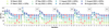 |
Fig. A.1 Illustration of the selection criterion used for order-wise SysRem optimisation for the CRIRES+ datasets. Here, the values of Δσ (vertical axis, where σ is the standard deviation of the residual matrix; see text) are plotted as a function of the SysRem pass (horizontal axis) across all spectral orders for observations from all six nights. Red stars mark the SysRem pass at which a plateau is reached, indicating the point at which the algorithm is halted. Spectral order number is indicated in the upper right corner of each cell. For clarity, an offset was added to the per-night curves, as indicated in the legend. |
 |
Fig. A.2 Cross-correlation matrices in the Earth’s rest frame for potential H2O signals in GJ 1214b as a function of the velocity Doppler shifts applied to the template (horizontal axis, full range explored) and the planet’s orbital phase (vertical axis). Results are shown per spectral order (columns) and for each night (rows). The H2O template employed presented 10× solar metallicity and a 10 mbar cloud deck. The red box marks an excluded spectral order due to uncorrected systematics. |
 |
Fig. A.3 Transit depth of H2O for GJ 1214 b in the analysed K band range as a function of cloud deck pressure level (top panel, fixed metallicity of 10× solar) and atmospheric metallicity (bottom panel, clear atmosphere) as multiples of solar. For clarity, an offset of 0.002 in transit depth was applied to the transmission models in both panels. |
 |
Fig. A.4 Same as Fig. 4, for each individual transit analysed and for the molecules studied. First row corresponds to water vapour, second row to methane, and third to carbon dioxide. |
The closest possible to the values Teff = 3026 K, log(g) = 5.026, and [Fe/H] = 0.29 from Cloutier et al. (2021).
All Tables
All Figures
|
Fig. 1 volution of the airmass, relative humidity, and mean S/N per spectrum. The pink-shaded area marks the in-transit times. Nodding A spectra are represented with empty symbols and Nodding B spectra with filled symbols. |
| In the text | |
|
Fig. 2 Steps of the data preparation applied to a representative spectral region of the dataset obtained on the night of 31 March 2022. The vertical axis in panel A represents flux in arbitrary units, while in all other panels it represents time, expressed as the planet’s orbital phase. Panel A: original spectrum observed at mid-transit, where telluric absorption lines from H2O can be identified. Panel B: original spectral matrix extracted using CR2RES, where major S/N differences between spectra (horizontal stripes) and prominent telluric H2O absorption (vertical stripes) can be identified. Panel C: normalised and masked spectra, where opaque telluric windows are excluded (white stripes). Panel D: residual spectra after one SysRem pass, where telluric residuals can be observed. Panel E: residual spectra after nine SysRem passes, where most of the telluric contribution has been removed. Nodding position effects were corrected in all panels by interpolating the pixelwavelength solution from nodding position B to position A. |
| In the text | |
|
Fig. 3 Cross-correlation analysis of potential H2O signals in the transmission spectrum of GJ 1214 b observed with CRIRES+ in the nearinfrared. The method is illustrated for the night of 31 March 2022. We show the cross-correlation matrix in the Earth’s rest frame as a function of the velocity Doppler shifts applied to the template (horizontal axis) and the planet’s orbital phase (vertical axis). The results were obtained by using a template with 10× solar metallicity and a 10 mbar cloud deck. All useful spectral orders were combined. White lines mark the transit start and end times, while the yellow lines indicate the expected exoplanet velocities with respect to Earth. |
| In the text | |
|
Fig. 4 Significance analysis of potential H2O signals, illustrated for the night of 31 March 2022. Top panel: S/N map as a function of radial velocity in the exoplanet’s rest frame (vrest, horizontal axis) and the projected orbital velocity semi-amplitude, Kp (vertical axis). Horizontal lines mark the expected Kp, and vertical lines show the zero rest-frame velocity. Bottom panel: 1D cross-correlation function at the expected Kp (97.1 kms−1)of GJ 1214b. |
| In the text | |
|
Fig. 5 Cross-correlation maps in S/N units for potential atmospheric signals as a function of vrest and Kp for the primary expected absorbing species in the atmosphere of GJ 1214 b. We explored water vapour (left), methane (middle), and carbon dioxide (right). Horizontal and vertical red lines indicate the expected Kp and vrest. These example maps were derived using a 10× solar metallicity template with a cloud deck at 10 mbar. No molecular signals were detected in our cross-correlation analyses. |
| In the text | |
|
Fig. 6 Transit depth of the main absorbers (H2, He, H2O, CO2, CO, CH4, NH3, and H2S) for GJ 1214 b in the analysed K band range as a function of cloud deck pressure level (top panel, fixed metallicity of 10× solar) and atmospheric metallicity (bottom panel, clear atmosphere) as multiples of solar. For clarity, an offset of 0.002 in transit depth was applied to the transmission models in both panels. |
| In the text | |
|
Fig. 7 Detectability maps obtained from injection-recovery tests, showing upper limits on the abundances of the main near-infrared strongest absorbers in the atmosphere of G 1214 b. Specifically, we investigate H2O (left panel), CH4 (middle panel), and CO2 (right panel) across a range of metallicities and cloud deck altitudes. Dashed lines indicate the S/N = 5 contours for H2O, CH4, and CO2, as obtained from CRIRES+ (white, eight transits combined). The lower S/N of CO2 recoveries stems from its weaker and fewer lines in the K band, compared to the other infrared absorbers. Red dotted lines indicate the upper limits derived in Kempton et al. (2023) from day and nightside evidences of H2O observed with JWST, in the best-fitting case of reflective clouds and high metallicity. |
| In the text | |
|
Fig. 8 Simulated detectability maps of GJ 1214 b computed with EXoPLORE, assuming a single-transit observation with ANDES on the upcoming ELT. We compute the case of H2O (left), CH4 (middle), and CO2 (right). The white (only for CH4) and red contours indicate recovered S/N levels of 10 and 5 in ANDES in silico data, respectively. For comparison purposes, we also include the S/N = 5 curves (black) obtained from the empirical data analysed in this work (Fig. 7). |
| In the text | |
|
Fig. A.1 Illustration of the selection criterion used for order-wise SysRem optimisation for the CRIRES+ datasets. Here, the values of Δσ (vertical axis, where σ is the standard deviation of the residual matrix; see text) are plotted as a function of the SysRem pass (horizontal axis) across all spectral orders for observations from all six nights. Red stars mark the SysRem pass at which a plateau is reached, indicating the point at which the algorithm is halted. Spectral order number is indicated in the upper right corner of each cell. For clarity, an offset was added to the per-night curves, as indicated in the legend. |
| In the text | |
|
Fig. A.2 Cross-correlation matrices in the Earth’s rest frame for potential H2O signals in GJ 1214b as a function of the velocity Doppler shifts applied to the template (horizontal axis, full range explored) and the planet’s orbital phase (vertical axis). Results are shown per spectral order (columns) and for each night (rows). The H2O template employed presented 10× solar metallicity and a 10 mbar cloud deck. The red box marks an excluded spectral order due to uncorrected systematics. |
| In the text | |
|
Fig. A.3 Transit depth of H2O for GJ 1214 b in the analysed K band range as a function of cloud deck pressure level (top panel, fixed metallicity of 10× solar) and atmospheric metallicity (bottom panel, clear atmosphere) as multiples of solar. For clarity, an offset of 0.002 in transit depth was applied to the transmission models in both panels. |
| In the text | |
|
Fig. A.4 Same as Fig. 4, for each individual transit analysed and for the molecules studied. First row corresponds to water vapour, second row to methane, and third to carbon dioxide. |
| In the text | |
Current usage metrics show cumulative count of Article Views (full-text article views including HTML views, PDF and ePub downloads, according to the available data) and Abstracts Views on Vision4Press platform.
Data correspond to usage on the plateform after 2015. The current usage metrics is available 48-96 hours after online publication and is updated daily on week days.
Initial download of the metrics may take a while.