© The Authors 2026

1. Introduction

The modelling of energy transport, mixing of chemical elements, and excitation and damping of waves due to free, buoyancy-driven convection is a major challenge in stellar physics (Weiss et al. 2004; Kupka & Muthsam 2017) as well as in the related disciplines of planetary sciences and geophysics (see Mironov 2009 for a review on numerical weather predictions). This statement also holds when neglecting the interactions of convection with rotation and with magnetic fields (reviewed in Brun & Browning 2017). For stellar evolution, the modelling of convection limits the accuracy and precision of determinations made with respect to pre-main sequence evolution tracks as well as stellar radii during the main sequence and later stages of stellar evolution. Its interaction with nucleosynthesis and the mixing of chemical elements throughout stellar evolution restrains the predictive capability of stellar models (for an introduction, see Hansen et al. 2004 and Kippenhahn et al. 2012). The modelling of convection is also important to helio- and asteroseismology since convection drives and damps stellar pulsation, and it can be probed by seismology (Houdek & Dupret 2015; Christensen-Dalsgaard 2021).

Mixing length theory (MLT; Biermann 1932; Böhm-Vitense 1958) has long remained the standard model for stellar convection (Weiss et al. 2004). Its long-lasting success (cf. Hansen et al. 2004 and Salaris & Cassisi 2005) has been accompanied by the discovery of an increasing number of its limitations. These include convective overshooting and its impact on the main sequence turn-off in stellar clusters (VandenBerg et al. 2006) as well as on the HR diagram location of eclipsing binaries (Claret & Torres 2019). The structural surface effect discovered in the analysis of the discrepancies between observed and predicted frequencies of solar p-modes is a term specifically invented to describe a major failure of MLT based solar models (see Christensen-Dalsgaard 2002, Houdek & Dupret 2015, Christensen-Dalsgaard 2021) and similar mismatches can be found for sound speed predictions at the bottom of the solar convection zone (Christensen-Dalsgaard et al. 2011). This has partially been remedied by either calibrating the mixing length itself to match the specific entropy predicted by 3D numerical simulations (Spada et al. 2021) or by replacing the predictions for the stellar surface layers with averages from 3D hydrodynamical simulations altogether, a technique know as model patching (Rosenthal et al. 1999; Mosumgaard et al. 2020). This approach is limited to modelling stellar surface layers, since for the deep stellar interior the thermal relaxation of 3D hydrodynamical simulations becomes unaffordable (Kupka & Muthsam 2017).

A revisit to a long known alternative is hence worthwhile, namely, towards non-local models of convection that require the construction of differential equations for predicting statistical properties of the dynamical variables describing convection, such as the velocity, u, and temperature, T. Examples of these include the models of Gough (1977), Xiong (1978), Stellingwerf (1982), Kuhfuß (1986), Xiong et al. (1997), Canuto (1992, 1997, 2009, 2011), and Li (2012). In each, the non-linearity of the advection operator in the Navier-Stokes equations leads to a closure problem: higher order moments have to be expressed in terms of lower order ones to derive a closed set of dynamical equations for the statistical properties of turbulent flows (Pope 2000).

Non-local models of convection have often been used in 1D modelling of stellar pulsation, but less frequently in stellar evolution models. Models used in practice mostly add just one dynamical equation to the equations describing the mean structure of the star (one equation models). Examples used in stellar pulsation and stellar evolution codes include the models of Stellingwerf (1982), Kuhfuß (1986), Roxburgh (1989), and Zahn (1991). A common additional dynamical variable is the turbulent kinetic energy. Its advection into or away from a local point is computed from a third-order moment (TOM), the flux of kinetic energy, F_kin. This was accounted for in the works of Stellingwerf (1982) and Kuhfuß (1986), whereby their models can also be used to model time-dependent changes of the stellar structure due to large amplitude radial pulsations. The models of Roxburgh (1989) and Zahn (1991) neglect F_kin, avoid an extra dynamical equation, and assign all non-radiative transport to the convective enthalpy flux, F_conv, which restricts them to stellar evolution modelling. In Stellingwerf (1982) and Kuhfuß (1986), F_kin is modelled as diffusion down a gradient. The idea of assuming a down-gradient model for all TOMs describing transport by advection was used by Xiong (1978, 1985, 1986) as well as independently by Kuhfuß (1986, 1987). It was also suggested by Canuto & Dubovikov (1998) as the most simple approach to close their Reynolds stress model of stellar convection.

Apart from the most simple one-equation models of convection, which neglect F_kin altogether, non-local models of turbulent stellar convection require statistical (closure) approximations of TOMs. A new model for the computation of the TOMs describing non-local transport was hence developed with the aim to overcome some of the limitations of the popular downgradient approximation (DGA). It is based on ideas previously suggested in meteorology (Zilitinkevich et al. 1999, Gryanik & Hartmann 2002, Gryanik et al. 2005). The latter required an external specification of the skewness of the fields of vertical velocity, w, and temperature, θ, S_w, and S_θ, respectively. To avoid this limitation, new models for S_w and S_θ were developed, which would allow for the construction of a complete closure of the TOMs, $\overline{w^3}$, $\overline{w^2\theta }$, and $\overline{w{\theta }^2}$, in terms of second-order moments and mean structure variables without the need to assume the plain DGA. Our model structure is described in Sect. 2 and its equations are given in Sect. 3. Consistency tests of the model based on 3D hydrodynamical simulations are presented in Sect. 4. Our discussion and conclusions on the modelling and its equations are given in Sects. 5 and 6.

2. Preparation of the model construction

The derivation of the model equations relies on several physical concepts, which we revisit in the following. They motivate the structure of the new models for the skewness of vertical velocity, S_w, and temperature, S_θ. Formally, S_w and S_θ are defined as

$$\begin{array}{cc}\hfill S_w& =\overline{w^3}/{\left(\overline{w^2}\right)}^{3/2},\hfill \end{array}$$(1)

$$\begin{array}{cc}\hfill S_{\theta }& =\overline{{\theta }^3}/{\left(\overline{{\theta }^2}\right)}^{3/2}.\hfill \end{array}$$(2)

The plain DGA assumes each TOM to just depend on a single gradient. Almost all applications of non-local models of convection in astrophysics have been based on that assumption. In three-equation models, which consist of dynamical equations for $\overline{w^2}$, $\overline{w\theta }$, and $\overline{{\theta }^2}$, the DGA is defined by the following equations:

$$\begin{array}{cc}\hfill \overline{w^2\theta }& =-D_1\partial \overline{w\theta }/\partial z,\hfill \end{array}$$(3)

$$\begin{array}{cc}\hfill \overline{w{\theta }^2}& =-D_2\partial \overline{{\theta }^2}/\partial z,\hfill \end{array}$$(4)

$$\begin{array}{cc}\hfill \overline{w^3}& =-D_3\partial \overline{w^2}/\partial z,\hfill \end{array}$$(5)

where the turbulent diffusivities, D_i, each depend on $\overline{w^2}$, a mixing length or dissipation timescale, and other local quantities. Several, very similar variants of this model have been suggested (see Xiong 1978, Kuhfuß 1987, or Canuto & Dubovikov 1998).

2.1. Mass flux models and statistical distribution functions

2.1.1. Coherent structures and their modelling

Convection itself is not necessarily turbulent. Firstly, convective instability in a fluid stratified by gravity (see Weiss et al. 2004, Hansen et al. 2004, or Kippenhahn et al. 2012) leads to up- and downflows along the directions of the oppositely acting forces of buoyancy and gravitation. Turbulence can be triggered by convection as a secondary effect such as friction at a solid surface as in the planetary boundary layer (PBL) of the atmosphere of the Earth (see Mironov 2009 for further reviews) or by shear forces between up- and downflows or horizontal shear stresses due to rotation. Each of these can give rise to a Kelvin-Helmholtz instability (Lesieur 2008) that, for sufficiently large length scales and/or velocities, can let the flow become turbulent. For convection in non-degenerate stars and in white dwarfs this is essentially always the case (see Muthsam et al. 2010 or Kupka & Muthsam 2017) and, thus, buoyancy becomes a source of turbulence (see Canuto & Dubovikov 1998, Canuto 2009).

Convection can also be driven just in a narrow region, where heat transport by conduction or radiation is strongly inhibited, as in the hydrogen and helium partial ionisation layers in the envelopes of cool stars. Alternatively, it may be driven in an extended region; for example, in the core region of massive stars where local heat production due to CNO cycle hydrogen-burning is high. The meteorological phenomena of dry convection above a heated terrestrial surface and moist convection in clouds (cf. Mironov 2009) are more closely related to the first case, for which observations as well as 3D numerical simulations have revealed the formation of large-scale coherent structures. These can be represented by a splitting into separate regions of up- and downflow. In meteorology, this has initiated the development of the mass flux model of convection (Arakawa 1969, Arakawa & Schubert 1974, see Mironov 2009 for a review). Once a flow has been set into motion it may readily pass through locally stable regions simply by Newton’s law of inertia (see Canuto 2009). Independently thereof, two-stream models had been suggested to better explain solar observations (see Ulrich 1970 and references therein) and more general two-component model stellar atmospheres had been developed in that period (Nordlund 1976). These models were based on observational constraints and on imposing physical conservation laws. In contrast, the MLT picture of a bubble moving along in an unstably stratified layer is tied to local linear stability analysis (Schwarzschild 1906) and therefore cannot provide a reliable prediction of flow topology, the extent of turbulently mixed regions, or the level of turbulence in a flow. The implications of the fundamentally non-local nature of stellar convection, as observed in the numerical simulations of Stein & Nordlund (1998), were discussed in Spruit (1997) and inspired a generalisation of MLT: it identifies surface cooling and the ‘entropy rain’ it generates as the main drivers of convection in stellar envelopes (Brandenburg 2016). The physical soundness of this concept has recently been corroborated by Käplyä (2025) who demonstrated by means of 3D numerical simulations of compressible convection that non-uniform, localised surface cooling drives deeply penetrating plumes as suggested by the model of Brandenburg (2016). Experimental evidence for narrow downflow regions deeply penetrating the upper solar convection zone has recently been suggested to result from interpretations of data obtained from local helioseismology (Hanson et al. 2024).

2.1.2. Filling factors, plume models, and skewness

Separately averaging over up- and downflows can be parametrised by a filling factor, σ, which represens the ratio of areas with upflow in a layer relative to its total area. This allows us to construct TOMs for non-local Reynolds stress models of convection (see Canuto & Dubovikov 1998 and the generalisation by Canuto et al. 2007), expressed as

$$\begin{array}{cc}\hfill \overline{w^2\theta }& =S_w\left({\overline{w^2}}^{1/2}\right)\overline{w\theta },\hfill \end{array}$$(6)

$$\begin{array}{cc}\hfill \overline{w{\theta }^2}& =S_w\left({\overline{{\theta }^2}}^{1/2}\right)\overline{w\theta },\hfill \end{array}$$(7)

$$\begin{array}{cc}\hfill \sigma & =\frac{1}{2}(1-S_w{(4+S_w^2)}^{-1/2}).\hfill \end{array}$$(8)

In this model, σ is only a diagnostic quantity parametrised by S_w. Canuto & Dubovikov (1998) suggested to use the full TOM equation for $\overline{w^3}$ for its computation. This also requires to model the TOMs $\overline{q^{2}w}$ and $\overline{q^2\theta }$ in the same framework, where $\overline{q^2}=\overline{u^2}+\overline{v^2}+\overline{w^2}$ is the total specific turbulent kinetic energy and the sum of contributions by horizontal and vertical velocities, $\overline{u^2}+\overline{v^2}$ and $\overline{w^2}$, respectively. The equations for these TOMs were closed in Canuto & Dubovikov (1998) by the quasi-normal approximation (QNA) for fourth-order moments with eddy damping¹. An equation for $\overline{w^3}$ was obtained, which is a linear combination of the gradients for $\overline{w^2}$, $\overline{q^2}$, and $\overline{w\theta }$ multiplied with highly non-linear front factors. This allowed for the computation of S_w in terms of second-order moments and mean values. In spite of the algebraic form of Eqs. (6) and (7), in that model $\overline{w^2\theta }$ and $\overline{w{\theta }^2}$ become proportional to a linear combination of several gradients of second-order moments.

A physically more complete but also more complex alternative was suggested in Canuto & Dubovikov (1998) as well: to use the stationary limit full solution for the dynamical equations of the TOMs $\overline{w^3}$, $\overline{{\theta }^3}$, $\overline{w^2\theta }$, $\overline{w{\theta }^2}$, $\overline{q^{2}w}$, and $\overline{q^2\theta }$ closed by an eddy damped QNA, which can be expressed as a linear combination of all the gradients of the different second-order moments (Canuto 1993). Thus, both models suggested to compute the TOMs from linear combinations of gradients of second-order moments multiplied with highly non-linear algebraic expressions.

Based on the assumption of the mass flux approximation, independently of Canuto & Dubovikov (1998), Abdella & McFarlane (1997) also arrived at Eqs. (7)–(8) and suggested a simpler approximation to compute S_w. In the end, they arrived at a linear combination of gradients of second-order moments to compute the TOMs as well.

As discussed below, Eq. (6) is a much better model for $\overline{w^2\theta }$ than Eq. (3) provided S_w is not computed from a plain or generalised DGA model for $\overline{w^3}$. However, we note that Eq. (7) has an additional shortcoming. Mironov et al. (1999) noted that contrary to Eq. (6), it is not invariant under sign change of w or θ: for the product of $S_w\overline{w\theta }$, independently of the sign of θ, w can only be linked to non-negative contributions independently of its sign. This is how $\overline{w^2\theta }$ and its closure, Eq. (6), behave, but it is not valid for $\overline{w{\theta }^2}$. And vice versa, θ only leads to non-negative contributions in $\overline{w{\theta }^2}$; however, this is not the case for $S_w\overline{w\theta }$, where a sign change of θ implies identical sign changes on both sides of Eq. (6). To strengthen their argument Mironov et al. (1999) demonstrated that the flux of temperature fluctuations, $\overline{w{\theta }^2}$, in 3D large eddy simulations (LES) data as well as in measurements of the convective PBL of the atmosphere of the Earth shows a negative sign above the convectively unstable layer (i.e. in its overshooting zone), while Eq. (7) predicts the opposite. This happens in spite of a rather good agreement of this closure with the data throughout most of the interior of the convective zone. Their finding was independently confirmed in Kupka (2007) by means of 3D direct numerical simulations of fully compressible convection for both overshooting above and below convection zones. A similar problem was also reported by Kupka & Muthsam (2007a) for the DGA approximation of $\overline{w{\theta }^2}$, Eq. (4).

2.1.3. Probabilistic interpretation and two-scale mass-flux approximation

Zilitinkevich et al. (1999) suggested reinterpreting the bimodal model used for the derivation of Eq. (6) in terms of probabilities. The splitting into up- and downflows depending on the local sign of vertical velocity is associated with the computation of the probability to find a particular value in a horizontal layer. By subtracting the mean values of velocity and temperature from local values, assuming that basic conservation laws hold, and constructing the probability density function after averaging over areas of equal sign of w, they re-derived the result for $\overline{w^2\theta }$ obtained by Abdella & McFarlane (1997) and Canuto & Dubovikov (1998), Eq. (6). Zilitinkevich et al. (1999) also pointed out that any good closure model ought to have the following properties: dimension, tensor rank and type, symmetries including sign changes, and realizability should be identical for both the quantity to be modelled and its closure approximation. Mironov et al. (1999) used this probabilistic interpretation of Zilitinkevich et al. (1999) to remedy the sign symmetry problem of Eq. (7). They suggested to extend the bimodal model to a scenario with three different states and their associated probabilities and assigned a non-zero probability for cold updrafts to exist along hot updrafts and cold downdrafts. Accounting for this additional physical state they derived a new closure for $\overline{w{\theta }^2}$ :

$$\begin{array}{c}\hfill \overline{w{\theta }^2}\sim S_{\theta }\left({\overline{{\theta }^2}}^{1/2}\right)\overline{w\theta }.\end{array}$$(9)

Zilitinkevich et al. (1999) also suggested an extended advection plus diffusion closure for Eq. (6):

$$\begin{array}{c}\hfill \overline{w^2\theta }=a_1{S}_w\left({\overline{w^2}}^{1/2}\right)\overline{w\theta }-D_4\partial \overline{w\theta }/\partial z.\end{array}$$(10)

This suggestion² was based on the notion that both Eq. (6) and Eq. (3) cannot be reduced to each other. Equation (6) represents perfect mixing with no vertical gradients, while the opposite case leads to strong gradients. These two cases are irreducible: in a perfectly mixed flow, there are no gradients and, thus, the DGA and the eddy damped QNA would predict the TOMs to be zero while Eqs. (6) and (9) can remain non-zero. This relates to the entropy rain model of Brandenburg (2016) and, as discussed for the convective (enthalpy) flux in Canuto (2009, per Eqs. 37 and 38) a convective heat flux may be generated in a thin layer and transported over extended distances without requiring a driving gradient in the region through which the energy is transported.

Such a flow state has also been called ballistically stirred by Gryanik & Hartmann (2002). Their work introduced the two-scale mass-flux approximation (TSMF) which suggests separate averaging for each of the different combinations of signs for w and θ, four in total. This means to also account for hot downflows in addition to the states considered in Mironov et al. (1999). For the TOMs, they recovered the closures of Zilitinkevich et al. (1999) and Mironov et al. (1999). They additionally suggested adding gradient diffusion to the closure for $\overline{w{\theta }^2}$,

$$\begin{array}{c}\hfill \overline{w{\theta }^2}=a_2{S}_{\theta }\left({\overline{{\theta }^2}}^{1/2}\right)\overline{w\theta }-D_5^{\prime }\partial \overline{{\theta }^2}/\partial z.\end{array}$$(11)

In addition, this is in agreement with Zilitinkevich et al. (1999), who noted (based on comparisons with numerical simulations of the PBL of the Earth atmosphere) that a₁ = 1 and a₂ = 1 yields sufficiently accurate results. Gryanik & Hartmann (2002) also suggested closures for many of the fourth-order moments based on the two-scale mass-flux approach and their approach was further generalised in Gryanik et al. (2005) to horizontal velocities. A very good agreement for these models was found in comparisons of the model predictions with aircraft measurements of the PBL and numerical simulations³ in the original papers. The models were also successfully validated in oceanography (Losch 2004) and with 3D hydrodynamical simulations of surface convection in the Sun and a main sequence K dwarf (Kupka & Robinson 2007). Confirming previous authors Cai (2018) found the TSMF model to outperform the QNA when probing it with 3D numerical simulations of compressible convection by a factor of two. Kupka & Robinson (2007) also noticed that the best of the two-scale mass-flux closures of Gryanik & Hartmann (2002) was the one for $\overline{w{\theta }^2}$, expressed by Eq. (11); this was followed by the one for $\overline{w^2\theta }$, expressed as Eq. (10), even without added gradient diffusion terms. They noted ‘a nearly perfect match’ when the latter were included. The excellent performance of Eq. (6) was also shown in Kupka & Muthsam (2017), who analysed 3D hydrodynamical simulations of solar surface convection with open vertical boundary conditions and simulations of a thin convection zone embedded in thick radiative zones in a DA white dwarf. They also demonstrated for Eq. (6) that it is of secondary importance whether Favre averages are used in the computation: $\overline{\rho w^2\theta }/\overline{\rho }$ and $\overline{w^2\theta }$ generally agree to better than 5%. Even at the superadiabatic peak, their difference is less than 20%.

In spite of their excellent performance these closures have not been used in calculations of stellar evolution, as they require accurate models for S_w and S_θ to outperform DGA-based closures. Kupka & Muthsam (2007a) and Kupka (2007) concluded from their direct numerical simulation of compressible convection that the DGA and the stationary limit full solution for the TOMs yield unsatisfactory results for $\overline{w^3}$, particularly for the case of a convection zone that is three pressure scale heights deep, along with poor results for $\overline{w^2\theta }$ and $\overline{w{\theta }^2}$ for all configurations of convective zones tested. The overall results for thin convective zones are acceptable when using the stationary limit full solution (Kupka 1999, Kupka & Montgomery 2002, Montgomery & Kupka 2004), since $\overline{w^2\theta }$ and $\overline{w{\theta }^2}$ are less important in that case⁴. In contrast, with S_w and S_θ taken from the numerical simulations, the performance of Eqs. (10)–(11) is an order of magnitude better than that of Eqs. (3)–(4) and for both, the correct sign changes are recovered.

2.2. The skewness of vertical velocity and temperature

A new model for S_w and S_θ was hence constructed which contains an additive term that cannot be reduced to a linear combination of gradients of second-order moments with multiplicative factors. This additive splitting into an algebraic term and a diffusion-type term was motivated by extending several arguments provided in Zilitinkevich et al. (1999) and Canuto (2009). Driving of convection within a narrow region as free convection occurs independently of the presence of shear stresses. It can be present even in physical systems with a laminar convective flow. Strong shear stresses in turn can lead to convective heat transport in systems with forced convection, with overshooting as a special case, and for situations without a clear correlation between up- and downflows as well as hot and cold flows. From a probabilistic viewpoint these two flow states can be driven simultaneously. Due to their different origins, however, they can be considered as independent of each other, which allows for irreducible states. The main hypothesis assumed in the new model is that this holds in general: interactions (including extreme events as discussed in Pratt et al. 2017) are sufficiently rare and (to a first approximation) they can be neglected. Thus, the free convective (algebraic) and the forced (diffusion) contribution can be added, each of them equipped with leading multiplicative closure constants to adjust their contributions in the transition (interpolation) regime, as done⁵ in the case of Eqs. (10)–(11).

A 3D LES of compressible convection by Chan & Sofia (1996) provided first guidance for modelling S_w. They found the closure $\overline{w^3}\approx -1.45{\left(\overline{w^2}\right)}^{3/2}$ or S_w ≈ −1.45 to work quite well for the lower four pressure scale heights of the convective zone. Deviations were reported to be large near the top of the convective zone and in the overshooting region. Equations (6) and (9) were not tested. Generally, they found pure algebraic closures to perform better inside the convection zone. The opposite was concluded for diffusion-type closures. Remarkably, the closure $\overline{w^3}\approx -1.9{\left(\overline{w^2}\right)}^{1/2}\ell \partial w^2/\partial z$ with ℓ = H_p, the local pressure scale height, worked well where the algebraic closure performed poorly and vice versa: the DGA closure underestimated S_w inside the convective zone and worked well near its boundary and in the overshooting zone. When adding both, the algebraic closures should dominate inside the convective zone and be negligible in the overshooting region. This is indicative for

$$\begin{array}{c}\hfill \overline{w^3}=a_3{\left(\overline{w^2}\right)}^{3/2}+d_6{\left(\overline{w^2}\right)}^{1/2}\ell \partial \overline{w^2}/\partial z,\end{array}$$(12)

with a₃ ≈ −1.5 and d₆ < 0 to be a first model for S_w. Equation (12) can violate sign symmetry and its algebraic contribution remains constant independently of stratification. A solution to this limitation is suggested in Sect. 3. In the work by Kupka & Robinson (2007), S_w is in the range of –1.4 to –1.5 within the first two pressure scale heights below the superadiabatic peak for a solar surface simulation; whereas it is closer to –1.25 for their K dwarf simulation and, thus, making it even more strongly influenced by the closed vertical bottom boundary. With open vertical boundaries, S_w is usually between –1.5 to –1.8 in the interior of the solar convection zone (see Belkacem et al. 2006 and Appendix D) and saturates at this value for several pressure scale heights. For narrow convection zones embedded in stably stratified layers, no plateau was found as the overshooting layers directly interact with the entire convection zone. Even in that case, a mean value around –1.5 appears to be realistic (cf. Kupka & Muthsam 2017).

Numerical 2D and 3D simulations of convection in the deep stellar interior (Dethero et al. 2024) and theoretical considerations motivated by 3D direct numerical simulations of convection (Yokoi et al. 2022; Yokoi 2023) indicate that both spatial and temporal correlations influence non-local transport and the filling factor σ and the skewness, S_w. No simple predictive model for the computation of S_w, however, could be derived as of now and a more complete model would likely introduce additional, dynamical equations for $\overline{w^3}$ and other quantities, which is beyond the scope of the present work.

Comparing computations of S_θ from 3D RHD in Belkacem et al. (2006), Kupka & Robinson (2007), and Kupka et al. (2018) this quantity is found to behave similar to S_w inside convective zones, where w and θ are well correlated, as follows from

$$\begin{array}{c}\hfill C_{w\theta }=\frac{\overline{w\theta }}{{\left(\overline{w^2}\overline{{\theta }^2}\right)}^{1/2}},\end{array}$$(13)

with positive values in the range of 0.7 to 0.85 in those layers (see also Chan & Sofia 1996). Thus, S_θ < 0 within stellar convection zones driven by cooling at the surface and |S_θ|≈1.4 |S_w| (cf. Belkacem et al. 2006 and Kupka & Robinson 2007). This becomes more intricate for thin convective zones (Kupka et al. 2018). To keep this first model simple, S_θ was constructed on the basis of S_w, so that the dimension, tensor rank, sign symmetry, and realizability are preserved, as reported in Sect. 3.

3. Derivation of the model equations

3.1. A model for S_θ to close $\overline{w{\theta }^2}$ in terms of S_w or $\overline{w^3}$

A simple closure for $\overline{{\theta }^3}$ in terms of $\overline{w^3}$ can be argued from dimensional constraints and sign symmetries: $\overline{w^2\theta }$ is invariant under w → −w and changes sign if θ → −θ. The relation

$$\begin{array}{c}\hfill \overline{{\theta }^3}\sim \overline{w^2\theta }\frac{\overline{{\theta }^2}}{\overline{w^2}}\end{array}$$(14)

fulfils both and inserting Eq. (6) into $\overline{w^2\theta }$ in Eq. (14) results in

$$\begin{array}{c}\hfill \overline{{\theta }^3}\sim \overline{w\theta }\frac{\overline{w^3}}{{\left(\overline{w^2}\right)}^2}\overline{{\theta }^2}.\end{array}$$(15)

The contraction of the vectors $\overline{w\theta }$ and $\overline{w^3}$ in Eq. (15) ensures that $\overline{{\theta }^3}$ and, thus, S_θ are scalars.

The realizability of this model for S_θ is more obvious, if it is re-derived by analysing the sign changes in S_θ, S_w, and $\overline{w\theta }$, as well as the convective and kinetic energy fluxes, F_conv and F_kin, in a 3D radiation hydrodynamical (RHD) simulation of a DA white dwarf with T_eff = 11800 K from Kupka et al. (2018). Horizontal averages of the simulation data over an extended time series reveal a sign change for F_conv at simulation box depths of ≈0.75 km and ≈2.8 km (with F_conv > 0 within that range; see Fig. 3 in the cited work, where the convectively unstable zone is located within 1 km…2 km, with vertical distances measured from the top of the simulation box). In the same dataset, the cross-correlation, $\overline{w\theta }$, and the auto-correlation function, $C_{w\theta }=\overline{w\theta }/{(\overline{w^2}\overline{{\theta }^2})}^{1/2}$, display a sign change also at ≈2.8 km and a near-change in sign⁶ (C_wθ < 0.03) at ≈0.7 km. Furthermore, S_w has a negative sign between ≈0.2 km and ≈5.1 km as has F_kin (see their Figs. 3 and 11). Outside that region |F_kin|≲10⁻⁵ F_total. Another observation is that S_θ < 0 between ≈1 km and ≈2.8 km (see their Fig. 11); that is, roughly where S_w < 0 and C_wθ > 0 and, thus, S_wC_wθ < 0, too. Below ≈2.8 km, S_θ > 0 and due to the sign change for C_wθ, this agrees with S_wC_wθ > 0. Above the convective zone, the relation between S_θ and S_wC_wθ is more complex, but this zone is subject to strong radiative cooling and non-radiative flux contributions are very small. From this analysis, the relation

$$\begin{array}{c}\hfill S_{\theta }=a_4{C}_{w\theta }{S}_w,\end{array}$$(16)

with 1 ≲ a₄ ≲ 2 appears to be a useful first approximation in regions where non-radiative energy flux contributions are higher in magnitude than 0.1% of the total flux. Both sides of Eq. (16) are dimensionless, featuring sign symmetry (invariant under w → −w and changing sign with θ → −θ), where the contraction of C_wθ S_w is a scalar as is S_θ; if S_w is realizable, so is S_θ, since |C_wθ|≤1 by the Cauchy-Schwarz inequality and realizability can always be ensured by choosing a value for a₄ that is not too large. If Eq. (15) is divided by ${(\overline{{\theta }^2})}^{3/2}$ and a₄ is inserted on its right-hand side to replace similarity with equality, it is easy to see that Eq. (15) is equivalent to Eq. (16). If Eq. (16) is used in Eq. (11) to eliminate S_θ and for generality a₂ a₄ is replaced by a₅, a new closure for $\overline{w{\theta }^2}$ is obtained which no longer depends explicitly on $\overline{{\theta }^3}$, but it does respect sign symmetries, contrary to Eq. (7). Its algebraic term is expressed as

$$\begin{array}{c}\hfill \overline{w{\theta }^2}=a_5{\left(\overline{w\theta }\right)}^2\overline{w^3}{\left(\overline{w^2}\right)}^{-2}=a_5{S}_w{\left(\overline{w\theta }\right)}^2{\left(\overline{w^2}\right)}^{-1/2}\end{array}$$(17)

and it depends only on $\overline{w^3}$, $\overline{w^2}$, and $\overline{w\theta }$, as Eq. (6) does for $\overline{w^2\theta }$.

Following the arguments by Zilitinkevich et al. (1999), Mironov et al. (1999), and Gryanik & Hartmann (2002), and the discussion provided in Sect. 2.2, a gradient diffusion term should be added to Eq. (17) (D₅ can differ from D₅′ in Eq. 11) to obtain

$$\begin{array}{c}\hfill \overline{w{\theta }^2}=a_5{\left(\overline{w\theta }\right)}^2\frac{\overline{w^3}}{{\left(\overline{w^2}\right)}^2}-D_5\partial \overline{{\theta }^2}/\partial z,\end{array}$$(18)

which, contrary to Eq. (11), no longer depends on $\overline{{\theta }^3}$.

3.2. A model for S_w and $\overline{w^3}$ to close $\overline{w^2\theta }$ and $\overline{w{\theta }^2}$

To close S_w, Eq. (12) for $\overline{w^3}$ is first divided by ${(\overline{w^2})}^{3/2}$ to obtain

$$\begin{array}{c}\hfill S_w=a_3+d_6\ell {\overline{w^2}}^{-1}\partial \overline{w^2}/\partial z.\end{array}$$(19)

The quantity a₃ is not a universal constant. In principle, it is a function constrained by the conservation of mass, momentum, and energy as well as other physical requirements. Yet deriving a prognostic equation for a₃ (or S_w) would require adding a new, non-local and highly non-linear (partial) differential equation to the convection model. Given the status quo in convection modelling in stellar structure and stellar evolution theory, such a complex model could be seen as unviable, since numerical robustness is a requirement for the codes developed for this purpose and this is equally as important as is physical reliability. Thus, a simpler approach, which still provides an improvement an order of magnitude over Eq. (5), was considered. Accounting for a possible dependency on the Brunt-Väisälä frequency, $\stackrel{\sim }{N}$, defined in Eq. (21), we can generalise Eq. (19) as

$$\begin{array}{c}\hfill S_w=a_{6}f(\stackrel{\sim }{N},\ell ,\overline{w^2},\overline{q^2})+d_6\ell {\overline{w^2}}^{-1}\partial \overline{w^2}/\partial z,\end{array}$$(20)

where a₆ should be chosen in the range of −1.25 to −1.8, if the convective flow is driven by cooling at an upper boundary, in agreement with results from the literature (see Sect. 2.2). It could be chosen to be in the range 0 < a₆ ≲ 0.5, if the flow is driven by heating by a bottom boundary layer (as expected from the data of Mironov et al. 1999 and Gryanik & Hartmann 2002). It is set to 0 if neither applies. This does not resolve cases where a transition between these states occurs as a function of location or time. For convective envelopes, the first case applies. For convective cores the third case is more appropriate, but this requires further study with 3D numerical simulations. If both types of zones are coupled, the transition between both states has to be modelled.

In the following, we only consider the case of convective driving by cooling at an upper boundary. The most important correction to the non-diffusive part of the model is the introduction of a function $f(\stackrel{\sim }{N},\ell ,\overline{w^2},\overline{q^2}),$ such that f → 1, where $\stackrel{\sim }{N}=0$ and f → 0 far away from the convective zone, just as the dissipation rate length scale in the same region (Kupka et al. 2022). Due to the radial dependence of f and due to the gradient diffusion term the quantity S_w is not just constant with depth.

In Kupka et al. (2022) the dynamical equation for the dissipation rate of turbulent kinetic energy ϵ, suggested in Canuto & Dubovikov (1998), was used to account for how waves excited in stable stratification damp convective overshooting. This equation can also guide the modelling of f, since the plumes generated by free convection also excite the waves in stably stratified layers that draw off their kinetic energy. With $K=\overline{q^2}/2$, it is expressed as

$$\begin{array}{cc}\hfill {\partial }_tϵ+D_{\mathrm{f}}(ϵ)& =c_1ϵK^{-1}g{\alpha }_{\mathrm{v}}\overline{w\theta }-c_2{ϵ}^2{K}^{-1}+c_3ϵ\stackrel{\sim }{N},\hfill \\ \hfill \mathrm{with}\stackrel{\sim }{N}& \equiv \sqrt{g{\alpha }_{\mathrm{v}}|\beta |}={\tau }_{\mathrm{b}}^{-1},\hfill \end{array}$$(21)

for small Prandtl numbers and β = −((∂T/∂z)−(∂T/∂z)_ad) is the superadiabatic gradient, g is the local gravitational acceleration, α_v is the volume expansion coefficient, and $\stackrel{\sim }{N}$ is the Brunt-Väisälä frequency with its reciprocal (i.e. the buoyancy timescale, τ_b). The values c₁ = 1.44 and c₂ = 1.92 are roughly in the middle of the typical range of values suggested in Tennekes & Lumley (1972) and Hanjalić & Launder (1976). A value of c₃ = 0.3 was suggested in Canuto & Dubovikov (1998). Instead of considering the DGA for D_f(ϵ), the relations

$$\begin{array}{c}\hfill D_{\mathrm{f}}(ϵ)\equiv {\partial }_z(\overline{ϵw})\mathrm{and}\overline{ϵw}=\frac{3}{2}\frac{\overline{q^{2}w}}{2}\frac{1}{\tau }\end{array}$$(22)

from Canuto (1992, 2009) were found to be preferable in proceeding with the next steps. These relations performed very well when tested with 3D numerical simulations of convection in Kupka & Muthsam (2007b), who also found that the DGA failed to correctly predict $\overline{ϵw}$.

In the following, contrary to the explanation given by Kupka et al. (2022, in their Sects. 3.5 and 3.6) a slightly more accurate approximation was made for the stationary limit of Eq. (21) by considering Eq. (22) and approximating it as ${\partial }_z(\overline{ϵw})=(c_5/\ell )(3/4)(\overline{q^{2}w}/\tau )$ to arrive at

$$\begin{array}{c}\hfill \frac{3}{4}\frac{\overline{q^{2}w}}{\tau }\frac{c_5}{\ell }=2c_{1}g{\alpha }_{\mathrm{v}}\overline{w\theta }/\tau -2c_2ϵ/\tau +c_3ϵ\stackrel{\sim }{N},\end{array}$$(23)

instead of approximating the non-local contribution by D_f(ϵ)≈ − α_ϵϵ/τ. In the stably stratified region, once we also have F_conv < 0 (plume-dominated region), the buoyancy term, $2c_{1}g{\alpha }_{\mathrm{v}}\overline{w\theta }/\tau$, becomes small (cf. Fig. 8 in Kupka et al. 2022 and the discussion in their Sect. 3.6 of the results of Kupka & Montgomery 2002 and Montgomery & Kupka 2004). Thus, it was neglected or considered to be absorbed into −2 c₂ϵ/τ, as in Kupka et al. (2022). Recalling from Canuto & Dubovikov (1998) that the dissipation rate timescale, τ, is related to the dissipation rate length scale, ℓ,  and ϵ via τ = 2 K/ϵ, ϵ = c_ϵ K^3/2/ℓ, and τ = 2 ℓ/(c_ϵ K^1/2), hence ℓ = K^1/2 τ c_ϵ/2 with c_ϵ ≈ 0.8, it is possible to rewrite Eq. (23), after dividing by c₂ ϵ²/K, as

$$\begin{array}{c}\hfill \frac{3}{4}\overline{q^{2}w}\frac{c_5}{\ell \tau }\frac{K}{c_2{ϵ}^2}=-1+\frac{c_3}{2c_2}\frac{\tau }{{\tau }_{\mathrm{b}}}.\end{array}$$(24)

Ignoring the velocity asymmetry for the turbulent kinetic energy, $K=\overline{q^2}/2\approx (3/2)\overline{w^2}$, where we also have $\overline{q^{2}w}\approx 3\overline{w^3}$. This step tacitly assumes the skewness of the horizontal velocity components to equal that of vertical velocity. In a straightforward generalisation, we could instead model the skewness of the total velocity field $\overline{q^{2}w}/K^{3/2}$ and derive S_w from a model of non-isotropic flow. That step is not necessary for three-equation non-local models of convection, such as that of Kuhfuß (1987, discussed in Kupka et al. 2022) where isotropy of the velocity field is assumed. Hence, it was not further considered in the rest of this study. With these approximations, Eq. (24) was rewritten in terms of $\overline{w^3}$ into

$$\begin{array}{c}\hfill \frac{3}{8}\frac{c_5}{c_2}\frac{\overline{w^3}}{\overline{w^2}\ell {\tau }^{-1}}=-1+\frac{c_3}{2c_2}\frac{\tau }{{\tau }_{\mathrm{b}}}.\end{array}$$(25)

Introducing S_w instead of $\overline{w^3}$ and rearranging Eq. (25) yields

$$\begin{array}{c}\hfill \tau =\frac{2c_2}{c_3}(1+\sqrt{\frac{3}{8}}\frac{c_5}{c_2{c}_{ϵ}}{S}_w){\tau }_{\mathrm{b}}.\end{array}$$(26)

With c₄ = c₃/(c₂ c_ϵ))≈0.2 (see Kupka et al. 2022) and setting

$$\begin{array}{c}\hfill a_6^{\prime }=-\frac{c_2{c}_{ϵ}}{c_5}\sqrt{\frac{8}{3}},\end{array}$$(27)

while recalling that with $\overline{q^2}/2=K\approx (3/2)\overline{w^2}$ and a₆ ≈ a₆′, we have

$$\begin{array}{c}\hfill S_w=a_6(1-c_4\ell K^{-1/2}{\tau }_{\mathrm{b}}^{-1})=a_{6}f(\stackrel{\sim }{N},\ell ,\overline{w^2},\overline{q^2}),\end{array}$$(28)

as the result. It is important to note that the sign of c₅ in Eq. (23) was not constrained to be positive, because the term it appears in approximates the divergence of a flux, which can act as a source or a sink. For stellar envelope convection, a₆ can be taken from the range of −1.25 to −1.8 (as discussed above) and $f(\stackrel{\sim }{N},\ell ,\overline{w^2},\overline{q^2})=f({\tau }_{\mathrm{b}},\ell ,K)=1-c_4\ell K^{-1/2}{\tau }_{\mathrm{b}}^{-1}$. Moreover, at the transition to unstable stratification, $\stackrel{\sim }{N}=0$, where S_w = a₆ at that point.

If the model is used in a wide parameter range, $c_4\ell K^{-1/2}{\tau }_{\mathrm{b}}^{-1}\approx 1$ might not always hold in the limit $\stackrel{\sim }{N}\gg 0$ in an overshooting layer far away from the convective zone. For instance, this criterion is roughly satisfied for the solar granulation simulations discussed in Sect. 4, but it fails in the case of overshooting above and below a thin envelope convection zone of a DA white dwarf. This is because τ ≫ τ_b. To ensure that f → 0 for large $\stackrel{\sim }{N}$ a harmonic limiter was introduced into the model, which forces f to remain within [0, 1] for $c_4\ell K^{-1/2}{\tau }_{\mathrm{b}}^{-1}>0$ and guarantees f → 1 for $\stackrel{\sim }{N}\to 0$ and f → 0 for $\stackrel{\sim }{N}\to \infty$. As the harmonic limiter overestimates f, where $\stackrel{\sim }{N}\to 0$, c₄ should be replaced by c₆ with c₄/2 ≲ c₆ ≲ c₄. Returning to Eq. (20), the new model for S_w is finally expressed as

$$\begin{array}{cc}\hfill S_w& =a_6(1-\frac{2c_6\ell K^{-1/2}\stackrel{\sim }{N}}{1+2c_6\ell K^{-1/2}\stackrel{\sim }{N}})+d_6\ell {\overline{w^2}}^{-1}\frac{\partial \overline{w^2}}{\partial z}\mathrm{if}\stackrel{\sim }{N}>0,\hfill \\ \hfill S_w& =a_6+d_6\ell {\overline{w^2}}^{-1}\frac{\partial \overline{w^2}}{\partial z}\mathrm{otherwise},\hfill \end{array}$$(29)

with $\overline{w^2}=(2/3)K$, a₆ ≈ −1.5, 0.1 ≲ c₆ ≲ 0.2, and d₆ < 0 subject to further analysis with 3D RHD simulations. The closure model for $\overline{w^3}$ is suggested to be

$$\begin{array}{cc}\hfill \overline{w^3}& =a_6(1-\frac{2c_6\ell K^{-1/2}\stackrel{\sim }{N}}{1+2c_6\ell K^{-1/2}\stackrel{\sim }{N}}){\overline{w^2}}^{3/2}+d_6\ell {\overline{w^2}}^{1/2}\frac{\partial \overline{w^2}}{\partial z}\mathrm{if}\stackrel{\sim }{N}>0,\hfill \\ \hfill \overline{w^3}& =a_6{\overline{w^2}}^{3/2}+d_6\ell {\overline{w^2}}^{1/2}\frac{\partial \overline{w^2}}{\partial z}\mathrm{otherwise},\hfill \end{array}$$(30)

with a₆, c₆, and d₆ taken as for S_w. If the timescale τ = 2 K/ϵ is available (instead of ℓ, as in comparisons with numerical simulations), we can instead use the relations from Kupka et al. (2022). In this case, we would have

$$\begin{array}{c}\hfill c_4\ell K^{-1/2}\stackrel{\sim }{N}=(c_3/(2c_2))(\tau /{\tau }_{\mathrm{b}})=0.078125(\tau /{\tau }_{\mathrm{b}})\end{array}$$(31)

and

$$\begin{array}{c}\hfill c_4\ell K^{-1/2}\stackrel{\sim }{N}=c_4\sqrt{2/3}\ell {\overline{w^2}}^{-1/2}\stackrel{\sim }{N}=c_4^{\prime }\ell {\overline{w^2}}^{-1/2}\stackrel{\sim }{N},\end{array}$$(32)

with $c_4\sqrt{2/3}=c_4\prime \approx 0.16$, to rewrite the equations and compute S_w or $\overline{w^3}$ from Eq. (29) or Eq. (30). With Eq. (10) for $\overline{w^2\theta }$ and Eq. (18) for $\overline{w{\theta }^2}$ and Eq. (30) for $\overline{w^3}$, we obtained a closed set of equations for these three TOMs in terms of second-order moments and mean structure quantities. This new TOM model can be used to close three-equation non-local convection models, such as that of Kuhfuß (1987), with details also given in Kupka et al. 2022 and Ahlborn et al. 2022). Introducing $D_4=-d_4\ell \overline{w^2}$ and $D_5=-d_5\ell \overline{w^2}$, we can rewrite Eqs. (10) and (18) as

$$\begin{array}{c}\hfill \overline{w^2\theta }=a_1\overline{w^3}{\left(\overline{w^2}\right)}^{-1}\overline{w\theta }+d_4\ell \overline{w^2}\frac{\partial \overline{w\theta }}{\partial z},\end{array}$$(33)

$$\begin{array}{c}\hfill \overline{w{\theta }^2}=a_5\overline{w^3}{\left(\overline{w^2}\right)}^{-2}{\left(\overline{w\theta }\right)}^2+d_5\ell \overline{w^2}\frac{\partial \overline{{\theta }^2}}{\partial z},\end{array}$$(34)

where a₁ = 1, a₅ is in the range of 1 to 2, and d₄ < 0 as well as d₅ < 0 (as in case of a₅) have to be determined from comparisons with 3D numerical simulations of convection. Appendix A shows how to use these results to close the convection model of Kuhfuß (1987).

4. Testing the model

The new TOM model consists of Eqs. (30), (33), and (34) for $\overline{w^3}$, $\overline{w^2\theta }$, and $\overline{w{\theta }^2}$ and relations for the skewness of vertical velocity S_w and temperature S_θ, Eqs. (29) and (16). This new model was tested by means of 3D RHD simulation data and compared to several closure models from the literature. The model was required to agree with direct computations of the TOMs from the 3D RHD data when its closure expressions were evaluated with input data from the same source. A perfect closure would yield results nearly identical to a direct computation of the three TOMs as well as S_w and S_θ. This way the predictive capabilities of the new closure model were probed independently from other approximations made within standalone non-local convection models such as that of Kuhfuß (1987). The comparison models included, firstly, the DGA given by Eqs. (5), (3), and (4), and secondly, the model Eq. (11) for $\overline{w{\theta }^2}$ from Gryanik & Hartmann (2002) combined with the model of Zilitinkevich et al. (1999), Eq. (10), for $\overline{w^2\theta }$, which for convenience is referred to here as the TSMF model with DGA. The TSMF model was also tested without DGA terms (D₄ = 0 and D₅′ = 0), as suggested by several authors before (see Sect. 2.1). Equations (10) and (11) cannot be used self-consistently in non-local convection models unless S_w and S_θ are known from some other source. To benchmark the impact of Eq. (30) on the predictions of Eqs. (33) and (34), in the TSMF model with and without DGA terms the quantities S_w and S_θ were taken directly from the 3D RHD data.

For the test, we used three previously published numerical simulations: the first dataset was taken from a simulation of solar surface convection with closed upper and lower vertical boundaries (Kupka & Robinson 2007) performed with the code from Robinson et al. (2003). This simulation included only a rather shallow solar photosphere. Its closed vertical boundaries directly affect predictions of the behaviour of S_w, S_θ, and the TOMs as a function of depth in the simulation domain. A comparison with a simulation with vertically open boundary conditions enabled us to quantify their role. The model assumed a T_eff of 5777 K and a log g of 4.4377. The chemical composition is described in Kupka & Robinson (2007). The predictions of S_w of the different TOM models for this simulation are shown in Fig. 1 and further results are provided in Appendix B. The second dataset was obtained from a simulation of solar surface convection performed with the code of Muthsam et al. (2010) presented in Belkacem et al. (2019). It featured open vertical boundary conditions and a photosphere ranging almost 600 km above the layer where the average temperature equals the solar T_eff of 5777 K. It also assumed a log g of 4.4377. Details on the chemical composition and the T_eff measured from the simulation, found to be close to 5750 K, were given in Belkacem et al. (2019). Due to the limited accuracy of the TOM models such differences were not important for the test described below. Finally, 3D RHD simulation data of a DA white dwarf with a T_eff close to 11 800 K and a log g of 8 with a pure hydrogen composition were taken from a dataset discussed in Kupka et al. (2018). In that simulation, carried out with the code from Muthsam et al. (2010), the entire vertical extent of the convective zone, including its neighbouring overshooting regions, was contained completely inside the simulation domain.

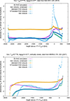Fig. 1. Skewness of vertical velocity Sw in 3D RHD simulations of solar granulation. Top: Open vertical boundary conditions at top and bottom (using the code of Muthsam et al. 2010). Bottom: Closed vertical boundary conditions (using the code of Robinson et al. 2003). Data directly computed from the 3D RHD numerical simulations (purple line with crosses) are compared with the new TOM model and the DGA. For the new TOM model, the green line with x-shaped points shows the no damping case (c6 = 0). The full, new model (c6 = 0.1) is indicated by a dark blue line with circles. The light brown line with asterisks denotes the DGA (d3 = −0.1). The light blue line with squares shows the DGA with ten times larger turbulent diffusivity (d3 = −1).

The closure parameters of the different TOM models were first roughly adjusted according to the simulation of Kupka & Robinson (2007) and then refined from tests with the data of Belkacem et al. (2019). The data from Kupka et al. (2018) were not considered in this process, apart from c₆, for which we chose to perform all the comparisons with a smaller value than that implied by the solar simulations. This was done to avoid an overestimated damping of the skewness in the extended Deardorff countergradient layer, which appears in the lower overshooting region of the DA white dwarf. After this process the values for these parameters were not adjusted any further. The values used for all the results shown in Figs. 1–5 are summarised in the following. For the DGA, the diffusivities had been defined as $D_1=-d_1\ell \overline{w^2}$ and $D_2=-d_2\ell \overline{w^2}$, as well as $D_3=-d_3\ell \overline{w^2}$. Keeping the relevant applications to stellar evolution calculations in mind, ℓ was computed similarly to the approach in Kupka et al. (2022) and Ahlborn et al. (2022), using τ = 2 K/ϵ and ϵ = c_ϵ K^3/2/ℓ with c_ϵ = 0.8 and Λ taken from their model. This was not crucial since, for the cases shown in Figs. 1–5, the alternative choice of Λ = 1.5 H_p was found to yield qualitatively and quantitatively similar results⁷. The values d₁ = −0.01, d₂ = −0.01, and d₃ = −0.1 allow for the positive diffusivities, D₁, D₂, and D₃, to be multiplied with a negative gradient in Eqs. (3), (4), and (5), as required by the model⁸.

As already mentioned, the TSMF model was used as a reference for the computation of $\overline{w^2\theta }$ and $\overline{w{\theta }^2}$ with the new TOM model. It was used in its original form, via Eqs. (6) and (9) or, equivalently, Eqs. (10) and (11) with a₁ = 1, a₂ = 1, D₄ = 0, and D₅′ = 0. It was also used with additional gradient terms (denoted as TSMF closure + DGA term in the following) based on Eqs. (10) and (11), where a₁ = 1, a₂ = 1, while $D_4=-d_4\prime \ell \overline{w^2}$ and $D_5\prime =-d_5\prime \ell \overline{w^2}$ with d₄′= − 0.04 and d₅′= − 0.01. Especially the choice of d₄′ improved model predictions at the solar surface.

For the new TOM model, a value of a₄ = 1.5 was used for the computation of S_θ according to Eq. (16). This is right in the middle of the suggested range discussed in Sect. 3.1. Taking a₂ = 1, the relation a₅ = a₂ a₄ (discussed in Sect. 3.1) would imply a₅ = 1.5. Since Eq. (34) for the computation of $\overline{w{\theta }^2}$ in the new model also has a downgradient contribution, a smaller value of a₅ = 0.5 turned out to yield better results. In comparison with Eq. (4), the downgradient contribution was increased by setting d₅ = −0.06. This accounts for changes introduced by the evaluation of Eq. (34) when $\overline{w^3}$ is computed from Eq. (30), instead of taking it directly from the 3D RHD data (which, on the contrary, must be done for the TSMF model). The coefficients in Eq. (33) for the computation of $\overline{w^2\theta }$ with $\overline{w^3}$ taken from Eq. (30) were set to a₁ = 0.6 and d₄ = −0.06, a similar change to that employed in the case of $\overline{w{\theta }^2}$. The solutions based on the new TOM model were all computed by means of Eq. (30) with $a_6=-\sqrt{2}$ and d₆ = −0.2. The choice of a₆ was motivated by the realizability constraint for the kurtosis of vertical velocity, K_w ≥ 1 + S_w², for skewed flow with a normal distribution, K_w = 3 (see Kupka & Robinson 2007). The extra damping by the harmonic limiter required c₆ = 0.1. Values closer to 0.2 improved the match for the 3D RHD in the solar photosphere but increased the differences in the lower countergradient layer of the DA white dwarf. Equation (31) was used to simplify comparisons with different computations for τ in 3D RHD numerical simulations. If the new TOM model were used in a non-local convection model with an isotropic velocity field, model coefficients might have to be scaled according to Eq. (32).

For Fig. 1, S_w was computed with the new closure with damping (c₆ = 0.1) as well as without (c₆ = 0) damping, then compared to the DGA and also a DGA solution with a diffusivity ten times larger and a direct computation from the 3D RHD simulation, each for the solar granulation simulations presented in Belkacem et al. (2019) and in Kupka & Robinson (2007). Clearly, the DGA completely failed to predict S_w and even if d₃ were boosted from −0.1 to −1, the better match inside the quasi-adiabatic convective zone were traded with a failure in size and sign at the top of the convective zone and in the photosphere. The closed boundary at the bottom of the 3D RHD by Kupka & Robinson (2007) led to somewhat larger discrepancies, but this is uncritical, since the solid plate boundary condition was not considered in the design of the models.

Figure 2 compares S_θ from the new model and predictions for $\overline{w^3}$ from the same set of models as in Fig. 1 with 3D RHD simulation data from Belkacem et al. (2019). For S_θ, Eq. (16) with a₄ = 1 and C_wθ S_w taken from the 3D RHD data was compared with a direct evaluation of the 3D RHD simulation and with a calculation based on the new closure Eq. (29) to compute S_w, assuming a₄ = 1.5 for evaluating Eq. (16). The latter provided an at least qualitatively acceptable approximation which, however, missed the maximum at the top of the convective zone. Differences at the bottom could also have been caused by properties of the boundary conditions. The prediction of $\overline{w^3}$ by the new TOM model was satisfactory also from a quantitative viewpoint; this is in contrast to the DGA, which missed the numerical range of values in the interior of the convective zone by an order of magnitude and it even mispredicted the sign of $\overline{w^3}$ at the top of the convective zone. This problem only worsened when boosting d₃.

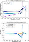Fig. 2. Skewness of temperature, Sθ (top), and TOM, $\overline{w^3}$ (bottom). The group of models displayed is the same as in the top panel of Fig. 1. Data are taken from the 3D RHD simulation with open vertical boundary conditions, as in the top of Fig. 1. The colour scheme is the same as in Fig. 1, except for the product of the cross-correlation of Cw, θ with Sw (shown here in dark blue with filled squares as points).

In Fig. 3, the predictions of the cross-correlations $\overline{w^2\theta }$ and $\overline{w{\theta }^2}$ are compared for the same models as for the case of $\overline{w^3}$ in Fig. 2; the exception is that no boosted DGA solutions are presented because they drastically fail anyway. Instead, the TSMF model with and without DGA term are shown. The data was again taken from the simulation of Belkacem et al. (2019). The DGA achieved acceptable results only for the top of the convective zone and the adjacent overshooting region. Inside the quasi-adiabatic interior of the convection zone, however, it failed to predict $\overline{w^2\theta }$ by an order of magnitude and $\overline{w{\theta }^2}$ by a factor of 3. The new model provided a much better prediction of both $\overline{w^2\theta }$ and $\overline{w{\theta }^2}$, which recovered the sign and the shape of these quantities as a function of depth. For the TSMF model with S_w and S_θ taken from the 3D RHD simulation the variant with a DGA contribution enabled a slightly better prediction of $\overline{w^2\theta }$ than the new model. Without this contribution, the TSMF failed to predict the correct sign of this quantity in the solar photosphere and performed worse than the new model. The DGA contribution to the TSMF model turned out to be much less important for $\overline{w{\theta }^2}$.

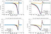Fig. 3. Comparisons for the TOMs $\overline{w^2\theta }$ (top) and $\overline{w{\theta }^2}$ (bottom). The simulation data and models are the same as those studied in Fig. 1 (top) and Fig. 2 (bottom) for Sw and $\overline{w^3}$, respectively: each panel displays results for the solar surface 3D RHD simulation with open vertical boundary conditions. The full vertical range is displayed in the left column of panels. The right column of panels zooms into the upper 40% of the simulation domain. The same colour coding was used as for Fig. 1. In addition, the results obtained for the TSMF closure with DGA (dark red line with asterisks) and without (dark green line with crosses) are shown. For both variants of the TSMF model, the quantity Sw was computed directly from 3D RHD data, as explained in the main text.

The white dwarf simulation of Kupka et al. (2018) provided an alternative test scenario which also included an extended countergradient layer and an overshooting zone underneath the convective zone. Figure 4 compares S_w, S_θ, $\overline{w^3}$, and a zoom into the upper half of the simulation domain for a more detailed analysis of the modelling of $\overline{w^3}$. The DGA, independently of whether d₃ = −0.1 or d₃ = −1, resulted in very poor predictions of S_w and $\overline{w^3}$. On the contrary, the new model recovered $\overline{w^3}$ very well. In the upper photosphere, damping by setting c₆ = 0.1 improved the comparison of the new TOM model with a direct computation of $\overline{w^3}$ over the choice c₆ = 0, whereas in the counter-gradient layer (between −1.3 km and −2 km for the chosen zero point of vertical depth), a weaker or no damping appears to be preferred. The results for S_w indicate that the lengthscale, Λ, used in the computation of the diffusivities of the downgradient contributions to $\overline{w^3}$ should drop more rapidly to allow for S_w → 0 in the wave-dominated region (see also Kupka et al. 2018). Further improvements were also found to be necessary to improve predictions of S_θ in the counter-gradient region. The results on the cross-correlations $\overline{w^2\theta }$ and $\overline{w{\theta }^2}$ shown in Fig. 5 confirmed the conclusions drawn from the solar case (Fig. 3). The DGA was not able to successfully predict their functional shape, magnitude, and sign. The new model achieved this goal to a much greater extent. It would even have been possible to achieve a match comparable with the TSMF model and the 3D RHD simulation by choosing a₁ = 1.2, instead of 0.6, and a₅ = 1.5, instead of 0.5, due to a much more realistic depth dependence of the new TOM model.

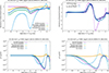Fig. 4. Skewnesses, Sw and Sθ, and the TOM, $\overline{w^3}$, in a 3D RHD simulation of convection in the upper envelope of a DA white dwarf. Top: Comparison of Sw (left) and Sθ (right) for the closure models discussed in Fig. 1 with input data taken from the 3D RHD simulation. The colour coding is the same as for Fig. 1 and 2. Bottom: Test of these closure models for the TOM $\overline{w^3}$ (left) alongside a zoom into the top half of the simulation domain (right). See a detailed discussion in the main text.

5. Discussion

Challenging its widespread use to compute the TOMs $\overline{w^3}$, $\overline{w^2\theta }$, and $\overline{w{\theta }^2}$, the DGA was probed with 3D RHD simulations of solar surface convection and a 3D RHD simulation of convection in the upper envelope of a DA white dwarf. Simulations of this kind had already passed a large variety of tests (see Nordlund et al. 2009, Kupka & Muthsam 2017, Kupka et al. 2018, Belkacem et al. 2019), which made them suitable for challenging closure models. The DGA was found to perform rather poorly in both cases, as it agreed with the 3D RHD simulations only near the boundary of convective regions and in neighbouring overshooting layers. In the interior of the convection zones, the DGA was found to differ by factors of three to ten from the simulation data and it even mispredicted the sign of $\overline{w^3}$ at the stellar surface including a positive flux of kinetic energy, F_kin > 0; whereas from 3D RHD simulations, this quantity was found to remain negative in the stellar photosphere, F_kin < 0, unless forced to do so by a closed upper boundary condition (see Appendix C).

The new TOM model developed in Sect. 3 was found to allow for a quantitative improvement over the DGA by up to an order of magnitude. The model also qualitatively improved the predictions of the TOMs $\overline{w^3}$, $\overline{w^2\theta }$, and $\overline{w{\theta }^2}$ by recovering, in most cases, their correct dependency as functions of depth and their correct sign. The same held for the skewness, S_w, even more so, when considering the large mismatch of the DGA for these quantities. Encouragingly, the same qualitative and quantitative improvements were found for both of the two rather different scenarios, solar surface granulation and shallow envelope convection in a DA white dwarf (Figs. 1–5). Further improvements might be required for the modelling of S_θ, where an additional contribution in the counter-gradient layer (Fig. 4, top-right panel) appears to be missing. Such improvements would also be needed to achieve a more efficient damping of the scale length, Λ, at the bottom of the lower overshooting zone (Fig. 4, top-left panel). The latter would ensure that S_w → 0 in the wave-dominated region. The modelling of $\overline{w{\theta }^2}$ could also benefit from such potential improvements, since for the DA white dwarf simulation, the latter was underestimated in magnitude, where |S_θ| was underestimated as well (see Figs. 4 and 5).

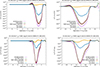Fig. 5. Testing closure models for the TOMs $\overline{w^2\theta }$ and $\overline{w{\theta }^2}$ with data of a 3D RHD simulation of envelope convection in a DA white dwarf. The same models as those given in Figs. 1 and 3 are used here. The case of the TOM $\overline{w^2\theta }$ is shown in the top row for the full vertical range (left) and for the upper half of the domain (right). For the line style and colour coding, see Fig. 3. The bottom row repeats this comparison for $\overline{w{\theta }^2}$. A discussion of the results is given in the main text.

The TSMF model was found to provide an even better approximation to the 3D RHD data, at least when extended with a DGA contribution, as suggested by Zilitinkevich et al. (1999) and Gryanik & Hartmann (2002). This was expected, since the new TOM model is based on approximations to S_w and S_θ, rather than taking their values directly from simulation data. However, for that same reason, the TSMF model cannot be used on its own in second-order closure non-local models of turbulent convection such as those by Kuhfuß (1987) and Kupka et al. (2022). Models using $\overline{w^3}$ to predict S_w for the TSMF model – which are based on the DGA or on more complete models that can be expressed as linear combinations of gradients of second-order moments (Canuto & Dubovikov 1998) or, additionally, TOMs (Gryanik & Hartmann 2002) – end up underestimating S_w because of the similar shape of all the gradients of the second-order moments; this prevents us from matching $\overline{w^3}$ and S_w simultaneously in the deep interior and at the convective zone boundary (see Appendices B and C). This shortcoming of gradient based models for S_w had already been observed in Kupka & Muthsam (2007a) and Kupka (2007) for direct numerical simulations of compressible convection and the conclusions on it do not change if density-weighted Favre averages are used instead of plain Reynolds averages: their small difference in computations of $\overline{w{\theta }^2}$ for solar surface granulation and envelope convection in DA white dwarfs was demonstrated in Kupka & Muthsam 2017 (see their Figs. 8 and 9). Moreover, in solar granulation simulations, the Favre averaged expression for F_kin (see Appendix C) features the same plateau as $\overline{w^3}$ (Fig. 1). Hence, the purely algebraic contributions contained in the new TOM model are a likely explanation for its improved performance, as described in Sect. 4.

It has to be emphasised here that the closure constants of the new TOM model (for lack of a more general theory from which it can be derived) should not be taken as an incentive to ‘fit’ any kind of astrophysical or other data ‘better’ than would otherwise be possible with the values suggested in Sect. 4. The concept proposed here is to calibrate them for a single case (as described in Sect. 4) and consider discrepancies among the observational data as an incentive to make further improvements on the functional form of the model.

It should also be noted that the seemingly ‘better’ performance of the DGA model in the wave-dominated region below the overshooting zone of the DA white dwarf envelope convection zone (Fig. 4, top-left panel) is solely due to the insufficiently damped scale length, Λ, in the gradient diffusivity appearing in both Eqs. (5) and (30) and the numerical values of d₃ and d₆ suggested in Sect. 4. Improving the model for Λ should solve this problem just as the discrepancies left for $\overline{{\theta }^3}$ and $\overline{w{\theta }^2}$ are best addressed by further improving the model for S_θ.

6. Conclusions

The accurate computation of non-local convective transport is one of the greatest challenges in building statistical models of solar and stellar structure and evolution (Kippenhahn et al. 2012). Such models are equally valuable to helio- and asteroseismology (Aerts et al. 2010; Houdek & Dupret 2015). They are also very important in oceanography and meteorology (Canuto 2009; Mironov 2009). The available models for the key quantities describing these processes (i.e. the TOMs of the vertical velocity and temperature or entropy) were usually found to have only a limited region of applicability (see the discussions in Losch 2004; Cheng et al. 2005; Cai 2018). For deep convective envelopes none of the available TOM models that require only second-order moments and mean quantities as input were found to be satisfactory (Chan & Sofia 1996; Kupka & Muthsam 2007a). Extending the ideas underlying the TSMF model (Gryanik & Hartmann 2002) and the entropy rain model (Brandenburg 2016), we propose a new model for the skewnesses, S_w and S_θ, and the TOMs, $\overline{w^3}$, $\overline{w^2\theta }$, and $\overline{w{\theta }^2}$, which is applicable to closing three equation non-local models of convection (Kuhfuß 1987; Kupka et al. 2022) designed for stellar evolution calculations. The new TOM model was found to provide a major qualitative and quantitative improvement over the DGA model currently used for this purpose.

Other plausible scenarios the model could be applied to include: the dry planetary boundary layer of the Earth, convective zones in the envelopes of giant planets, or the atmosphere of terrestrial planets, which can also feature driving by either convective cooling or heating (see Zilitinkevich et al. 1999 and references therein). However, the influence of solid, close boundaries may have to be considered more carefully and possibly the closure constants or at the very least the value of a₆ might have to be recalibrated (see also Sect. 3.2) on the basis of simulation data or measurements for such physical systems. Convection in clouds in turn would require to account for the effects of evaporation and condensation. For stellar astrophysics, the inclusion of effects of rotation on S_w is likely of more interest (as explored by Käplyä 2024).

The next steps in the development of the model include improvements to the modelling of the skewness, S_θ, and the associated third moments, $\overline{{\theta }^3}$ and $\overline{w{\theta }^2}$, as well as the scale length, Λ, to improve its predictive capabilities for S_w and S_θ, as well as to better account for anisotropy in convective flows, as summarised in Sect. 5. This will be followed up with the coupling of the new TOM model into a non-local model of convection for computing stellar envelopes. Finally, the model will be implemented into a stellar evolution code that would also allow us to account for the influence of rotation on non-local transport.

Acknowledgments

The author is thankful for the hospitality provided by the Wolfgang Pauli Institute, Vienna, and acknowledges support by the Faculty of Mathematics at the University of Vienna through offering him a Senior Research Fellow status. The Austrian Science Fund (FWF) has supported this research through grants P 33140-N, P 35485-N, and PAT1338425. Permission by F.J. Robinson to use his 3D simulation data for testing the new models is greatly appreciated.

References

Appendix A: A variant of the new TOM model for the Kuhfuß three-equation model of convection

To implement the TOM model as defined by Eqs. (30), (33), and (34) into the model of Kuhfuß (1987), used in the modification suggested by Kupka et al. (2022) and Ahlborn et al. (2022), Eq. (29) is rewritten in terms of the total turbulent kinetic energy ω ≡ K by means of Eq. (32). Differences due to isotropy assumptions are absorbed into the closure constants such that

$$\begin{array}{ccc}\hfill S_{\omega }& =\hfill & \hfill a_{\omega }(1-\frac{2{\stackrel{\sim }{c}}_6\ell {\omega }^{-1/2}\stackrel{\sim }{N}}{1+2{\stackrel{\sim }{c}}_6\ell {\omega }^{-1/2}\stackrel{\sim }{N}})+d_{\omega }\ell {\omega }^{-1}\frac{\partial \omega }{\partial z}\mathrm{if}N>0,\\ \hfill S_{\omega }& =\hfill & \hfill a_{\omega }+d_{\omega }\ell {\omega }^{-1}\frac{\partial \omega }{\partial z}\mathrm{otherwise}.\end{array}$$(A.1)

Furthermore. a_ω < 0, d_ω < 0, and ${\stackrel{\sim }{c}}_6$ have to be adjusted from the values for a₆, d₆, and c₆ provided in the main text. With $\overline{\rho }$ as the mean density the non-local flux F_ω can be computed from

$$\begin{array}{c}\hfill F_{\omega }=\frac{1}{\overline{\rho }}\mathrm{div}\left(S_{\omega }\overline{\rho }{\omega }^{3/2}\right).\end{array}$$(A.2)

The Kuhfuß (1987) model computes correlations for entropy fluctuations rather than temperature fluctuations. It hence requires to calculate the non-local fluxes of $\mathrm{\Pi }=\overline{ws\prime }$, which is the (radial component of the) flux of entropy fluctuations, closely related to the convective flux, and of $\varphi =\overline{s^{\prime 2}}$, the square of local entropy fluctuations. For a well mixed plasma in the temperature and density region of interest to stellar evolution calculations, the entropy fluctuations correlate very well with the temperature fluctuations of the fluid. Thus, the non-local fluxes of Π and ϕ are suggested to be obtained from Eqs. (33) and (34) by replacing θ with s′, setting v′² = q², and writing their non-local fluxes in terms of ω instead of w as follows:

$$\begin{array}{c}\hfill F_{\mathrm{\Pi }}=\frac{1}{\overline{\rho }}\mathrm{div}\left(\overline{\rho }\overline{v^{\prime 2}s\prime }\right)=\frac{1}{\overline{\rho }}\mathrm{div}\left(\overline{\rho }(a_{\mathrm{\Pi }}\mathrm{\Pi }{\omega }^{1/2}{S}_{\omega }+d_{\mathrm{\Pi }}\ell {\omega }^{1/2}\frac{\partial \mathrm{\Pi }}{\partial z})\right)\end{array}$$(A.3)

and

$$\begin{array}{c}\hfill F_{\varphi }=\frac{1}{\overline{\rho }}\mathrm{div}\left(\overline{\rho }\overline{v\prime s^{\prime 2}}\right)=\frac{1}{\overline{\rho }}\mathrm{div}\left(\overline{\rho }(a_{\varphi }{\mathrm{\Pi }}^2{\omega }^{-1/2}{S}_{\omega }+d_{\varphi }\ell {\omega }^{1/2}\frac{\partial \varphi }{\partial z})\right).\end{array}$$(A.4)

Again the constants a_Π > 0 and d_Π < 0 as well as a_ϕ > 0 and d_ϕ < 0 have to be adjusted from the values for a₁ and d₄ as well as a₅ and d₅ given in the main text.

Appendix B: 3D RHD simulations of solar convection with closed boundary conditions

Third-order and other higher order moments of the fluctuations, w and θ, of the basic variables velocity and temperature around an ensemble averaged mean state are sensitive to boundary conditions assumed for the spatial domain chosen for 3D RHD numerical simulations. To quantify their impact the tests of the new TOM model were also performed for a simulation of solar granulation that assumed a closed vertical boundary in the photosphere and a closed boundary with a small artificial heating zone inside the quasi-adiabatic envelope (Robinson et al. 2003; Kupka & Robinson 2007). A direct comparison with a 3D RHD simulation of solar granulation that allows for in- and outflow through the vertical boundary (Belkacem et al. 2019) was given in Fig. 1. Due to the solid plates of the 3D RHD simulation presented in Kupka & Robinson (2007)S_w did not feature a plateau in the interior of the quasi-adiabatic convective envelope of the Sun. At a distance of almost three local pressure scale heights from the bottom of the simulation domain |S_w| already begins to drop until it finally diverges towards the bottom. The DGA initially appears to follow this behaviour at least if the vertical turbulent momentum diffusivity were boosted by a factor of ten, but it diverges also much farther away from the lower boundary. A compromise could have been achieved by lowering |a₆| and increasing |d₆| in the new TOM model, though neither of the models was developed to account for the “solid plate scenario”. While the latter is of little interest to solar physics, an important lesson can be learned if the new TOM model were applied to the PBL of the Earth: the solid terrestrial surface could influence the vertical velocity field such that a constant skewness component could not be disentangled from a turbulent component. Indeed, in the PBL S_w slightly increases away from the bottom boundary (see Gryanik & Hartmann 2002 and Cheng et al. 2005) with no observable plateau, just as in the DA white dwarf simulation (Kupka et al. 2018) discussed in Fig. 4 in Sect. 4. The upper boundary of the simulation of Kupka & Robinson (2007) is also responsible for $\overline{w^3}$ changing sign near the top.

The top panel of Fig. B.1 demonstrates that these peculiarities caused by the closed boundary conditions can barely be noticed if $\overline{w^3}$ is considered. A very good match could have been achieved by slightly lowering |a₆| and doubling c₆ which would have lowered the contribution of the non-local (algebraic) component. The influence of the vertical boundary conditions is similar, if S_θ is considered instead of S_w (Fig. B.1, bottom panel).

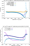Fig. B.1. Further investigation of the models for the TOM $\overline{w^3}$ and the skewness of temperature Sθ. The top panel shows $\overline{w^3}$ and the bottom one shows Sθ. The closure models as well as colour and line style coding are the same as in Fig. 2, but for the case of the 3D RHD simulation of solar surface convection with closed vertical boundary conditions.

Fig. B.2 and Fig. B.3 show that similar to $\overline{w^3}$ illustrated in Fig. B.1, the TOMs $\overline{w^2\theta }$ and $\overline{w{\theta }^2}$ computed from the 3D RHD simulations were reproduced quite well by the new TOM model without any parameter readjustments. The discrepancies between direct computations of S_w and S_θ from the simulation and their evaluation from a model with simulation data for second-order moments and mean quantities as input are similar to the case with open vertical boundary conditions illustrated in Fig. 3. This underlines the central role of a detailed modelling of the skewnesses S_w and S_θ for future improvements of the new TOM model.

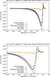Fig. B.2. Probing the TOM $\overline{w^2\theta }$ with 3D RHD solar simulation data for closed vertical boundary conditions. Details on the line style and colour coding are explained in the captions to Figs. 2 and 3. The top panel shows the full vertical depth range and the bottom panel shows a zoom into the upper 40% of that range.

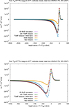Fig. B.3. Probing the TOM $\overline{w{\theta }^2}$ with 3D RHD solar simulation data for closed vertical boundary conditions. Details on the line style and colour coding can be found in the captions to Figs. 2 and 3. The top panel shows the full vertical depth range and the bottom one gives a zoom into the upper 40% of that range.

It is interesting to note that also for this case, each of the gradients of $\overline{w^2}$, $\overline{w\theta }$, and $\overline{{\theta }^2}$ has a similar shape, as it has for the cases discussed in Sect. 4. This shape prevents a proper match of $\overline{w^3}$ and S_w as well as $\overline{w^2\theta }$ and $\overline{w{\theta }^2}$ in the case of open upper boundary conditions. The same was found to hold for the 3D RHD simulation with closed vertical boundary conditions.

Appendix C: The computation of the flux of (turbulent) kinetic energy

An important physical quantity for the modelling of stellar evolution is the flux of turbulent kinetic energy, F_kin, which should enter into the flux balance of the luminosity equation of stellar evolution models (Canuto 1993). As a purely non-local quantity it cannot be computed within the framework of the mixing length theory of convection. In spite of its crucial role to allow for overshooting in first place (Canuto 1993) F_kin is not necessarily accounted for in the luminosity equation of stellar evolution codes. Figure C.1 can also be used to justify that decision: if the TOMs in the non-local convection model are computed from the DGA, |F_kin| barely exceeds 2% of the total energy flux and it might be argued for stability reasons that such a small quantity does not have to be accounted for. In such cases the non-local fluxes in the second-order moment equations still affect the computation of the convective enthalpy flux |F_conv| and thus the temperature gradient (the small amount given by |F_kin| is “absorbed” into F_conv in such models). As can also be seen from Fig. C.1, the assumption of a small |F_kin| no longer holds once this quantity is directly computed from 3D RHD numerical simulations of convection at the stellar surface and the upper part of the stellar envelope. The exact evaluation of F_kin is shown there as a bright red line with filled squares. It stays in the range of −15% to −20% of the total (actually input) flux throughout the quasi-adiabatic part of the convection zone in the solar case (top panel). A solid boundary inside such a zone necessarily forces F_kin back to zero (bottom panel), although even in this case it remains in this range except for the lowermost pressure scale height. For the 3D RHD simulation of the DA white dwarf even a value of −25% is attained and F_kin remains in the range of −20% to −5% throughout the countergradient layer. This is no longer a small contribution and an accurate prediction of the temperature structure in these classes of stars requires to account for its contribution to the energy flux budget.

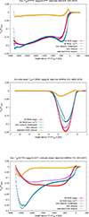Fig. C.1. Predictions of the flux of (turbulent) kinetic energy in three different 3D RHD simulations (top panel: solar case, middle panel: DA white dwarf; bottom panel: solar case with solid plate at the bottom). The same colour and linestyle coding is used as for Fig. 1. For the models and for the computation from only the vertical component of the kinetic energy flux an identical scaling factor of 2/3 was applied (see text in Appendix C). The evaluation of the exact expression for this quantity from the 3D RHD simulations is shown in bright red with data points denoted by filled squares.

When challenging TOM models to predict F_kin, the first problem to be solved is the computation of the triple correlation for the flux of the total kinetic energy, $\overline{q^{2}w}$. For Fig. C.1 this was done by testing whether $F_{\mathrm{kin}}=(1/2)\overline{\rho q^{2}w}$ could be estimated from $F_{\mathrm{kin}}\approx c_{\mathrm{Fkin}}\overline{\rho }\overline{w^3}$. Figure C.1 demonstrates that the latter is sufficiently accurate for all cases considered by simply setting c_Fkin = 2/3 (see also Chan & Sofia 1996). This is likely due to a rather constant anisotropy ratio between the total and the vertical (turbulent) kinetic energy. Deviations from that constancy can be neglected at the stellar surface due to the rapid drop of density which makes the contribution of F_kin to the total flux negligibly small. The same procedure was hence applied to estimate F_kin from the different models for $\overline{w^3}$. Again, the new TOM model performs very well except near the bottom of the “artificially” vertically closed solar surface convection simulation shown in the bottom panel of Fig. C.1. If the new TOM model is used in non-local stellar convection models, F_kin should hence be accounted for in the energy flux budget. It can safely be neglected, if the DGA model is used, since the latter completely underestimates this quantity, as already mentioned further above.

Appendix D: Arguments based on plume models

Plume models as developed in Canuto & Dubovikov (1998), Canuto et al. (2007), Canuto (2009), and also Belkacem et al. (2006) provide additional arguments for chosing the contribution to S_w created by cooling in a narrow boundary layer as a constant, Eq. (19), and scale $\overline{w^3}$ proportional to ${(\overline{w^2})}^{3/2}$ as in Eq. (12). As discussed in Canuto & Dubovikov (1998) Eq. (8) can easily be rewritten into $S_w=(1-2\sigma )/\sqrt{\sigma -{\sigma }^2}$ to yield S_w as a function of (upflow) area σ. For an upflow area fraction of 0.79 (and a downflow area fraction of 0.21) a value of $S_w=-\sqrt{2}\approx a_6$ is obtained (the choice of sign for S_w when solving this quadratic equation is straightforward). From an inspection of 3D RHD of solar granulation it follows (Belkacem et al. 2006) that values of S_w in the range of −1.75 to −1.5 are correlated with values of σ in the range of 0.67 to 0.63, whence Eq. (8) overestimates σ (or underestimates |S_w|). This can be attributed, among others, to the averaging procedure used in the two-delta function plume model (see Belkacem et al. 2006 for details). To account for such effects would require a dynamical equation for S_w and result in a significantly more complex model. Equation (14) for S_θ cannot be as easily motivated from the family of two-delta function plume models since they do not distinguish between S_w and S_θ as required from 3D RHD solar granulation simulations (Belkacem et al. 2006). The TSMF model of Gryanik & Hartmann (2002) does so by construction, which also lends support to the derivation of Eq. (16). The detailed dependencies between up- and downflows with hot and cold flows were simplified in Sect. 3.1, however, because this would have considerably increased the complexity of the model.

All Figures

Fig. 1. Skewness of vertical velocity Sw in 3D RHD simulations of solar granulation. Top: Open vertical boundary conditions at top and bottom (using the code of Muthsam et al. 2010). Bottom: Closed vertical boundary conditions (using the code of Robinson et al. 2003). Data directly computed from the 3D RHD numerical simulations (purple line with crosses) are compared with the new TOM model and the DGA. For the new TOM model, the green line with x-shaped points shows the no damping case (c6 = 0). The full, new model (c6 = 0.1) is indicated by a dark blue line with circles. The light brown line with asterisks denotes the DGA (d3 = −0.1). The light blue line with squares shows the DGA with ten times larger turbulent diffusivity (d3 = −1).

In the text

Fig. 2. Skewness of temperature, Sθ (top), and TOM, $\overline{w^3}$ (bottom). The group of models displayed is the same as in the top panel of Fig. 1. Data are taken from the 3D RHD simulation with open vertical boundary conditions, as in the top of Fig. 1. The colour scheme is the same as in Fig. 1, except for the product of the cross-correlation of Cw, θ with Sw (shown here in dark blue with filled squares as points).

In the text

Fig. 3. Comparisons for the TOMs $\overline{w^2\theta }$ (top) and $\overline{w{\theta }^2}$ (bottom). The simulation data and models are the same as those studied in Fig. 1 (top) and Fig. 2 (bottom) for Sw and $\overline{w^3}$, respectively: each panel displays results for the solar surface 3D RHD simulation with open vertical boundary conditions. The full vertical range is displayed in the left column of panels. The right column of panels zooms into the upper 40% of the simulation domain. The same colour coding was used as for Fig. 1. In addition, the results obtained for the TSMF closure with DGA (dark red line with asterisks) and without (dark green line with crosses) are shown. For both variants of the TSMF model, the quantity Sw was computed directly from 3D RHD data, as explained in the main text.

In the text

Fig. 4. Skewnesses, Sw and Sθ, and the TOM, $\overline{w^3}$, in a 3D RHD simulation of convection in the upper envelope of a DA white dwarf. Top: Comparison of Sw (left) and Sθ (right) for the closure models discussed in Fig. 1 with input data taken from the 3D RHD simulation. The colour coding is the same as for Fig. 1 and 2. Bottom: Test of these closure models for the TOM $\overline{w^3}$ (left) alongside a zoom into the top half of the simulation domain (right). See a detailed discussion in the main text.

In the text

Fig. 5. Testing closure models for the TOMs $\overline{w^2\theta }$ and $\overline{w{\theta }^2}$ with data of a 3D RHD simulation of envelope convection in a DA white dwarf. The same models as those given in Figs. 1 and 3 are used here. The case of the TOM $\overline{w^2\theta }$ is shown in the top row for the full vertical range (left) and for the upper half of the domain (right). For the line style and colour coding, see Fig. 3. The bottom row repeats this comparison for $\overline{w{\theta }^2}$. A discussion of the results is given in the main text.

In the text

	Fig. B.1. Further investigation of the models for the TOM $\overline{w^3}$ and the skewness of temperature Sθ. The top panel shows $\overline{w^3}$ and the bottom one shows Sθ. The closure models as well as colour and line style coding are the same as in Fig. 2, but for the case of the 3D RHD simulation of solar surface convection with closed vertical boundary conditions.
In the text

	Fig. B.2. Probing the TOM $\overline{w^2\theta }$ with 3D RHD solar simulation data for closed vertical boundary conditions. Details on the line style and colour coding are explained in the captions to Figs. 2 and 3. The top panel shows the full vertical depth range and the bottom panel shows a zoom into the upper 40% of that range.
In the text

	Fig. B.3. Probing the TOM $\overline{w{\theta }^2}$ with 3D RHD solar simulation data for closed vertical boundary conditions. Details on the line style and colour coding can be found in the captions to Figs. 2 and 3. The top panel shows the full vertical depth range and the bottom one gives a zoom into the upper 40% of that range.
In the text

Fig. C.1. Predictions of the flux of (turbulent) kinetic energy in three different 3D RHD simulations (top panel: solar case, middle panel: DA white dwarf; bottom panel: solar case with solid plate at the bottom). The same colour and linestyle coding is used as for Fig. 1. For the models and for the computation from only the vertical component of the kinetic energy flux an identical scaling factor of 2/3 was applied (see text in Appendix C). The evaluation of the exact expression for this quantity from the 3D RHD simulations is shown in bright red with data points denoted by filled squares.

In the text

References

- Abdella, K., & McFarlane, N. 1997, J. Atm. Sci., 54, 1850 [Google Scholar]
- Aerts, C., Christensen-Dalsgaard, J., & Kurtz, D. 2010, Asteroseismology, Astron. & Astrophys. Library (Heidelberg: Springer-Verlag) [Google Scholar]
- Ahlborn, F., Kupka, F., Weiss, A., & Flaskamp, M. 2022, A&A, 667, A97 [NASA ADS] [CrossRef] [EDP Sciences] [Google Scholar]
- Arakawa, A. 1969, in Proc. WMO/IUGG Symp. Numerical Weather Prediction, Vol. IV, 8 (Meteorological Agency: Japan), 1 [Google Scholar]
- Arakawa, A., & Schubert, W. H. 1974, J. Atoms. Sci., 31, 674 [Google Scholar]
- Belkacem, K., Kupka, F., Samadi, R., & Grimm-Strele, H. 2019, A&A, 625, A20 [EDP Sciences] [Google Scholar]
- Belkacem, K., Samadi, R., Goupil, M.-J., & Kupka, F. 2006, A&A, 460, 173 [CrossRef] [EDP Sciences] [Google Scholar]
- Biermann, L. 1932, Z. Astrophys., 5, 117 [NASA ADS] [Google Scholar]
- Böhm-Vitense, E. 1958, Z. Astrophys., 46, 108 [Google Scholar]
- Brandenburg, A. 2016, ApJ, 832, 6 [Google Scholar]
- Brun, A., & Browning, M. 2017, Liv. Rev. Sol. Phys., 14, 4 [NASA ADS] [CrossRef] [Google Scholar]
- Cai, T. 2018, ApJ, 868, 12 [Google Scholar]
- Canuto, V. M. 1992, ApJ, 392, 218 [Google Scholar]
- Canuto, V. M. 1993, ApJ, 416, 331 [NASA ADS] [CrossRef] [Google Scholar]
- Canuto, V. M. 1997, ApJ, 482, 827 [Google Scholar]
- Canuto, V. M. 2009, Lecture Notes Phys., 756, 107 [Google Scholar]
- Canuto, V. M. 2011, A&A, 528, A76 [NASA ADS] [CrossRef] [EDP Sciences] [Google Scholar]
- Canuto, V. M., Cheng, Y., & Howard, A. M. 2007, Ocean Mod., 16, 28 [Google Scholar]
- Canuto, V. M., & Dubovikov, M. 1998, ApJ, 493, 834 [NASA ADS] [CrossRef] [Google Scholar]
- Canuto, V. M., Minotti, F., Ronchi, C., Ypma, R. M., & Zeman, O. 1994, J. Atmos. Sci., 51, 1605 [NASA ADS] [CrossRef] [Google Scholar]
- Chan, K. L., & Sofia, S. 1996, ApJ, 466, 372 [NASA ADS] [CrossRef] [Google Scholar]
- Cheng, Y., Canuto, V. M., & Howard, A. M. 2005, J. Atmos. Sci., 62, 2189 [Google Scholar]
- Christensen-Dalsgaard, J. 2002, Rev. Mod. Phys., 74, 1073 [Google Scholar]
- Christensen-Dalsgaard, J. 2021, Liv. Rev. Sol. Phys., 18, 2 [NASA ADS] [CrossRef] [Google Scholar]
- Christensen-Dalsgaard, J., Monteiro, M. J. P. F. G., Rempel, M., & Thompson, M. J. 2011, MNRAS, 414, 1158 [CrossRef] [Google Scholar]
- Claret, A., & Torres, G. 2019, ApJ, 876, 134 [Google Scholar]
- Dethero, M.-G., Pratt, J., Vlaykov, D., et al. 2024, A&A, 692, A46 [NASA ADS] [CrossRef] [EDP Sciences] [Google Scholar]
- Gough, D. O. 1977, ApJ, 214, 196 [NASA ADS] [CrossRef] [Google Scholar]
- Gryanik, V. M., & Hartmann, J. 2002, J. Atmos. Sci., 59, 2729 [Google Scholar]
- Gryanik, V. M., Hartmann, J., Raasch, S., & Schröter, M. 2005, J. Atmos. Sci., 62, 2632 [Google Scholar]
- Hanjalić, K., & Launder, B. E. 1976, J. Fluid Mech., 74, 593 [CrossRef] [Google Scholar]
- Hansen, C. J., Kawaler, S. D., & Trimble, V. 2004, in Stellar Interiors. Physical Principles, Structure, and Evolution, 2nd edn. (Springer) [Google Scholar]
- Hanson, C. S., Das, S. B., Mani, P., Hanasoge, S., & Sreenivasan, K. R. 2024, Nat. Astron., 8, 1088 [Google Scholar]
- Houdek, G., & Dupret, M.-A. 2015, Liv. Rev. Sol. Phys., 12, 8 [Google Scholar]
- Käplyä, P. 2024, A&A, 683, A221 [NASA ADS] [CrossRef] [EDP Sciences] [Google Scholar]
- Käplyä, P. 2025, A&A, 698, L13 [NASA ADS] [CrossRef] [EDP Sciences] [Google Scholar]
- Kippenhahn, R., Weigert, A., & Weiss, A. 2012, Stellar Structure and Evolution, Astronomy and Astrophysics Library (Berlin Heidelberg: Springer-Verlag) [Google Scholar]
- Kuhfuß, R. 1986, A&A, 160, 116 [NASA ADS] [Google Scholar]
- Kuhfuß, R. 1987, Ph.D. Thesis, Max-Planck-Institut für Astrophysik, Technische Universität München [Google Scholar]
- Kupka, F. 1999, ApJ, 526, L45 [NASA ADS] [CrossRef] [Google Scholar]
- Kupka, F. 2007, IAU Symp., 239, 92 [Google Scholar]
- Kupka, F., Ahlborn, F., & Weiss, A. 2022, A&A, 667, A96 [NASA ADS] [CrossRef] [EDP Sciences] [Google Scholar]
- Kupka, F., & Montgomery, M. H. 2002, MNRAS, 330, L6 [NASA ADS] [CrossRef] [Google Scholar]
- Kupka, F., & Muthsam, H. J. 2007a, IAU Symp., 239, 83 [Google Scholar]
- Kupka, F., & Muthsam, H. J. 2007b, IAU Symp., 239, 86 [Google Scholar]
- Kupka, F., & Muthsam, H. J. 2017, Liv. Rev. Comp. Astrophys., 3, 1 [NASA ADS] [CrossRef] [Google Scholar]
- Kupka, F., & Robinson, F. J. 2007, MNRAS, 374, 305 [Google Scholar]
- Kupka, F., Zaussinger, F., & Montgomery, M. H. 2018, MNRAS, 474, 4660 [NASA ADS] [CrossRef] [Google Scholar]
- Lesieur, M. 2008, Turbulence in Fluids, 4th edn. (Dordrecht: Springer) [Google Scholar]
- Li, Y. 2012, ApJ, 756, 37 [NASA ADS] [CrossRef] [Google Scholar]
- Losch, M. 2004, Geophys. Res. Lett., 31, L23301 [Google Scholar]
- Millionshchikov, M. D. 1941, Dokl. Acad. Nauk SSSR, 32, 611 [Google Scholar]
- Mironov, D. V. 2009, Lecture Notes Phys., 756, 161 [Google Scholar]
- Mironov, D. V., Gryanik, V. M., Lykossov, V. N., & Zilitinkevich, S. S. 1999, J. Atmos. Sci., 56, 3478 [Google Scholar]
- Montgomery, M. H., & Kupka, F. 2004, MNRAS, 350, 267 [NASA ADS] [CrossRef] [Google Scholar]
- Mosumgaard, J., Jørgensen, A., Weiss, A., Aguirre, V., & Christensen-Dalsgaard, J. 2020, MNRAS, 491, 1160 [Google Scholar]
- Muthsam, H., Kupka, F., Löw-Baselli, B., et al. 2010, NewA, 15, 460 [Google Scholar]
- Nordlund, Å. 1976, A&A, 50, 23 [NASA ADS] [Google Scholar]
- Nordlund, Å., Stein, R. F., & Asplund, M. 2009, Liv. Rev. Sol. Phys., 6, 2 [Google Scholar]
- Pope, S. B. 2000, Turbulent Flows (Cambridge: Cambridge University Press) [Google Scholar]
- Pratt, J., Baraffe, I., Goffrey, T., et al. 2017, A&A, 604, A125 [NASA ADS] [CrossRef] [EDP Sciences] [Google Scholar]
- Robinson, F. J., Demarque, P., Li, L. H., et al. 2003, MNRAS, 340, 923 [Google Scholar]
- Rosenthal, C. S., Christensen-Dalsgaard, J., Nordlund, Å., Stein, R. F., & Trampedach, R. 1999, ApJ, 351, 689 [Google Scholar]
- Roxburgh, I. W. 1989, A&A, 211, 361 [NASA ADS] [Google Scholar]
- Salaris, M., & Cassisi, S. 2005, Evolution of Stars and Stellar Population (Wiley) [Google Scholar]
- Schwarzschild, K. 1906, Nachr. Koenigl. Gesellsch. Wiss. Goettingen, Math.-Phys. Kl., 195, 41 [Google Scholar]
- Spada, F., Demarque, P., & Kupka, F. 2021, MNRAS, 504, 3128 [NASA ADS] [CrossRef] [Google Scholar]
- Spruit, H. C. 1997, Mem. Soc. Astron. It., 68, 397 [NASA ADS] [Google Scholar]
- Stein, R. F., & Nordlund, Å. 1998, ApJ, 499, 914 [Google Scholar]
- Stellingwerf, R. F. 1982, ApJ, 262, 330 [NASA ADS] [CrossRef] [Google Scholar]
- Tennekes, H., & Lumley, J. L. 1972, in A First Course in Turbulence (M.I.T. Press) [Google Scholar]
- Ulrich, R. K. 1970, Astrophys. Space Sci., 9, 80 [Google Scholar]
- VandenBerg, D. A., Bergbusch, P. A., & Dowler, P. D. 2006, ApJS, 162, 375 [NASA ADS] [CrossRef] [Google Scholar]
- Weiss, A., Hillebrandt, W., Thomas, H.-C., & Ritter, H. 2004, Cox& Giuli’s Principles of Stellar Structure. Extended, 2nd edn. (Cambridge: Cambridge Scientific Publishers) [Google Scholar]
- Xiong, D. R. 1978, Chin. Astron., 2, 118 [NASA ADS] [CrossRef] [Google Scholar]
- Xiong, D. R. 1985, A&A, 150, 133 [NASA ADS] [Google Scholar]
- Xiong, D. R. 1986, A&A, 167, 239 [NASA ADS] [Google Scholar]
- Xiong, D. R., Cheng, Q. L., & Deng, L. 1997, ApJS, 108, 529 [NASA ADS] [CrossRef] [Google Scholar]
- Yokoi, N. 2023, Atmosphere, 14, 1013 [Google Scholar]
- Yokoi, N., Masada, Y., & Takiwaki, T. 2022, MNRAS, 516, 2718 [Google Scholar]
- Zahn, J.-P. 1991, A&A, 252, 179 [NASA ADS] [Google Scholar]
- Zilitinkevich, S., Gryanik, V. M., Lykossov, V. N., & Mironov, D. V. 1999, J. Atmos. Sci., 56, 3463 [Google Scholar]
The QNA of fourth-order moments by Millionshchikov (1941) assumes that all even order moments that are higher than the second order are normally distributed. This allows for the closure of the dynamical equations related to the TOMs (cf. Canuto 1992). To ensure realisability, the TOMs either have to be flux limited or eddy damping has to be applied to the pressure correlations in their dynamical equations (see Lesieur 2008). The advanced non-local model of deep convection by Canuto et al. (2007) also avoids the simple QNA.
Originally, another additive term proportional to the superadiabatic gradient was suggested. Following Mironov et al. (1999) and Gryanik & Hartmann (2002), it was neglected in the present study.
It is interesting to note that for the PBL the non-Gaussian contribution can be accounted for through proper eddy damping (Cheng et al. 2005), an approach which also ends up computing the TOMs from linear combinations of gradients of second-order moments.
Its good agreement found in Canuto et al. (1994) and Cheng et al. (2005) for the PBL could also be related to a much smaller depth d ≲ 0.125Hp and the different boundary conditions (solid bottom plate).
Cheng et al. (2005) found the predictions for  of the model of Gryanik & Hartmann (2002) to deviate from 3D simulation data near the top of the PBL. This agrees with the latter stating that entrainment (overshooting) layers are outside the region of applicability for their fourth-order moment closure model.
Compressibility, non-local radiative cooling, and the sensitivity of Cwθ to boundary conditions could explain that difference. Moreover, the non-radiative fluxes up there are small, with |Fconv|≲10−3 Ftotal.
This is explained by the radius dependence of the model of Kupka et al. (2022) for Λ. The model predicts a strong damping of Λ in the overshooting region of convective cores, but this effect is much weaker near the surface of main sequence stars with a radius R, where Hp ≪ R.
By introducing Di > 0 and di < 0 the DGA model could be written in its standard notation. This simplified the comparison with the new TOM model.