| Issue |
A&A
Volume 708, April 2026
|
|
|---|---|---|
| Article Number | A240 | |
| Number of page(s) | 7 | |
| Section | The Sun and the Heliosphere | |
| DOI | https://doi.org/10.1051/0004-6361/202658943 | |
| Published online | 09 April 2026 | |
Identification of periodic density structures in Solar Orbiter data: Helical structures and flux ropes
1
Department of Physics, National and Kapodistrian University of Athens, Athens, Greece
2
NASA-Goddard Space Flight Center, Greenbelt, MD, USA
3
Physics Department, The Catholic University of America, Washington, DC, USA
4
Department of Physics and Astronomy, University of Delaware, Newark, DE, USA
5
ESA/ESAC, Madrid, Spain
★ Corresponding author: This email address is being protected from spambots. You need JavaScript enabled to view it.
Received:
13
January
2026
Accepted:
17
March
2026
Abstract
Context. Quasi-periodic density structures (PDSs) are quasiperiodic variations in the solar wind density that range from a few minutes to a few hours. They are trains of advected density structures with radial length scales LR ≈ 100 − 10 000 Mm, and they thus belong to the class of so-called mesoscale structures in the solar wind. Although the precise mechanisms that form PDSs are still debated, cumulative evidence from multiple studies using in situ and remote data supports the view that most PDSs have a solar origin and do not form through dynamics during their propagation in interplanetary space. Low-frequency (< 1 mHz) PDSs have been associated with small-scale flux ropes, which further indicates a solar origin.
Aims. We further investigated the origin and properties of PDSs by searching for coherent small-scale helical structures and flux ropes within PDS intervals.
Methods. We used an extensive list of PDSs, compiled from Solar Orbiter measurements, and we applied a wavelet analysis technique to obtain the reduced magnetic helicity, cross helicity, and residual energy.
Results. Our results indicate that small flux ropes are a constituent of PDS events, while the occurrence probability of helical Alfvénic structures is similar within and outside the PDSs.
Conclusions. These results are consistent with the scenario in which PDSs are formed by processes involving magnetic reconnection.
Key words: Sun: magnetic fields / solar wind
© The Authors 2026
 Open Access article, published by EDP Sciences, under the terms of the Creative Commons Attribution License (https://creativecommons.org/licenses/by/4.0), which permits unrestricted use, distribution, and reproduction in any medium, provided the original work is properly cited.
This article is published in open access under the Subscribe to Open model. This email address is being protected from spambots. You need JavaScript enabled to view it. to support open access publication.
1. Introduction
Quasi-periodic density structures (PDSs) are so-called mesoscale structures in the solar wind and are a particular constituent of the ambient solar wind (Viall et al. 2021). Their frequencies span the range of 0.1 to 5 mHz, corresponding to radial length scales of 100−10 000 Mm, with the train of PDSs lasting from several hours to over a day. Although less frequently studied, their azimuthal size scales have been estimated to span the range of ≈1500−2600 Mm and ≈800−1800 Mm for PDSs with frequencies lower and higher than 1 mHz, respectively (Sanchez-Diaz et al. 2017; Di Matteo et al. 2024). These structures can affect global magnetospheric (Borovsky & Denton 2006) and radiation belt dynamics because of the direct changes to the solar wind dynamic pressure that are created by the changing proton number density (Viall et al. 2009; Di Matteo et al. 2022; Kurien et al. 2024). Therefore, it is very important to study their generation mechanisms and their propagation, not only to understand the daily driving of geospace but also to the wider space physics community.
The precise generation mechanism of PDSs is still debated. A generation en route via processes such as turbulence is considered, but also generation in the solar atmosphere (Viall et al. 2021). Several remote-sensing observations of the Sun supported the conclusion that PDSs have a solar origin (Viall & Vourlidas 2015; Ventura et al. 2023; Alzate et al. 2024). Low-frequency (< 1 mHz) PDSs in particular have been observed as outward-propagating density blobs in the solar atmosphere in coronagraph observations down to ≈2.0 solar radii (Viall & Vourlidas 2015; DeForest et al. 2018; Alzate et al. 2024). Magneto-hydrodynamic (MHD) simulations showed that the < 1 mHz PDSs may result from the periodic release of flux ropes from the tip of helmet streamers as a result of the tearing instability (Allred & MacNeice 2015; Réville et al. 2020; Schlenker et al. 2021; Poirier et al. 2023). Furthermore, in situ observations from 0.3 to 1.0 AU have also confirmed solar origin theories involving magnetic reconnection and interchange reconnection in the solar corona (Antiochos et al. 2011; Higginson & Lynch 2018). In- situ observations of small flux ropes associated with PDSs (Kepko et al. 2016; Di Matteo et al. 2019; Lavraud et al. 2020) are a key observable, suggesting reconnection as the most probable source. Katsavrias et al. (2024) recently investigated the thermodynamic signature of < 1 mHz PDS using Wind measurements. The authors found that coherent PDSs (a subset of PDS events with a similar periodic behaviour in proton density and α/p ratio) exhibited a sub-adiabatic polytropic index, similar to that of the magnetic flux rope in interplanetary coronal mass ejections (ICMEs). This result further strengthens the association of < 1 mHz PDSs with reconnection at the tip of the streamer that leads to the formation of small flux ropes.
We apply a wavelet analysis technique (Torrence & Compo 1998) to construct spectra of normalized reduced magnetic helicity, cross helicity, and residual energy based on the magnetic field and plasma measurements of Solar Orbiter. This technique has the advantage that it can identify Alfvénic structures and quasi-static magnetic flux ropes, and was previously applied to observations at 1 AU (Good et al. 2022) and closer to the Sun (Zhao et al. 2020). This method allowed us to investigate the existence of such structures within PDS intervals for the first time and to this extent, and it provides insights into the origin and evolution of PDSs.
2. Data and methods
2.1. Data
We used the total ion distributions and solar wind speed in radial-transverse-normal (RTN) coordinates from the Proton and Alpha particle Sensor (PAS; Owen et al. 2020), as well as magnetic field data from the magnetometer instrument (MAG; Horbury et al. 2020) on board the Solar Orbiter spacecraft, spanning the period of 2021–2024. The resolution of the PAS and MAG data was averaged to a cadence of 20 s.
To identify Alfvénic structures and quasi-static magnetic flux ropes, we exploited the Katsavrias & Di Matteo (2025a) PDS list, which is publicly available1 and includes PDSs identified using three window intervals of 6, 12, and 18 hours each (Katsavrias et al. 2026). We only used the < 1 mHz PDSs, which correspond to 1727, 2185, and 1895 events each for the three window intervals. Finally, for each PDS event, we derived the normalized reduced magnetic helicity (σm), the normalized cross helicity (σc), and the residual energy (σr), following the method reported by Telloni et al. (2012) and Zhao et al. (2020). We note that we used three different time intervals to be able to identify a PDS based on the trade-off between frequency resolution and PDS duration. Empirically, we found that 6 h segments are better for identifying high-frequency PDS (> 1 mHz), while the lower-frequency PDS (< 1 mHz) are best observed at longer window lengths. In this way, robustness was added to the statistical analysis by testing the consistency of the results across the various window lengths.
2.2. Derivation of the normalized reduced magnetic helicity (σm), normalized cross helicity (σc), and residual energy (σr)
The strict definition of the magnetic helicity density is that it is the dot product of the magnetic vector potential and the magnetic field, which depends on the spatial properties of the magnetic field topology and thus cannot be directly evaluated from single spacecraft measurements. However, a reduced form of magnetic helicity can be estimated using measurements from a single spacecraft based on the magnetic field power spectrum (Matthaeus et al. 1982). To derive the power spectrum, we used the continuous wavelet transform (CWT; Torrence & Compo 1998) and the Morlet wavelet (Morlet et al. 1982) as the mother wavelet on each component of the fluctuating magnetic field BR, BT, and BN (see also Katsavrias et al. 2012, 2022 for more details on CWT) as
![Mathematical equation: $$ \begin{aligned} \sigma _m=\frac{2\cdot \mathrm{Im}\left[W^{*}_{T}(f,t)\cdot W_{N}(f,t)\right]}{\left| W_{R}(f,t)\right|^2 + \left| W_{T}(f,t)\right|^2 + \left| W_{N}(f,t)\right|^2} \end{aligned} $$](/articles/aa/full_html/2026/04/aa58943-26/aa58943-26-eq1.gif) (1)
(1)
where f is the frequency, Wi(f, t) are the wavelet transforms of the time series of BR, BT, and BN, and  denotes the conjugate of WT (Telloni et al. 2012). The absolute values of σm are no higher than 1, and a positive value of σm corresponds to right-handed chirality and a negative value to left-handed chirality.
The normalized cross helicity, σc, and the residual energy, σr, were calculated from the Elsässer variables z± = u ± b, with  , where B is the magnetic field vector, np is the proton density, and mp is proton mass. z± represents the forward and backward propagating wave modes with respect to the magnetic field orientation, and their squares represent the energy density in forward- and backward-propagating modes (e.g., Bruno & Carbone 2013). The equations for σc and σr are given as
 (2)
(2)
and
 (3)
(3)
In order to derive the σc and σr spectrograms, we performed the CWT on the three components of the Elsässer variables, zR±, zT±, and zN±. The spectrogram of the normalized cross helicity is then written as
 (4)
(4)
and the spectrogram of the normalized residual energy is written as
![Mathematical equation: $$ \begin{aligned} \sigma _r = \frac{2\cdot \mathrm{Re}\left[W^{*}_{z^+_R}\cdot W_{z^-_R} + W^{*}_{z^+_T}\cdot W_{z^-_T} + W^{*}_{z^+_N}\cdot W_{z^-_N}\right]}{W^{+}+W^{-}} \end{aligned} $$](/articles/aa/full_html/2026/04/aa58943-26/aa58943-26-eq7.gif) (5)
(5)
where W± = |WzR±|2 + |WzT±|2 + |WzN±|2 represent the wavelet power spectrum in z± modes.
Similar to σm, the absolute values of σc and σr are no higher than 1. The magnitude of σc indicates the alignment between the velocity and magnetic field vector. This means that unidirectional Alfvén waves usually have a high value of σc. Furthermore, the sign of σc represents the direction of the propagating wave modes, where plus and minus correspond to more energy residing in forward- and backward-propagating wave modes, respectively. Finally, σr represents the energy difference between the fluctuating kinetic and magnetic energies, with σr > 0 corresponding to the dominating magnetic fluctuating energy and σr < 0 to the dominating kinetic fluctuating energy. Alfvén waves usually have a typical σr < 0 close to zero.
This method was applied to all the available PDS events, where we searched for structures with |σm|≥0.7, henceforth referred to as helical structures (HSs). We further isolated the intervals of HSs for which (a) the central time, tc, was within the PDS time limits, that is, tPDS, start < tc < tPDS, end, and (b) the mean frequency fell within the range of fPDS ± 0.15 mHz. The latter condition accounts for the uncertainty in the PDS frequency estimation using the MTM and wavelet methods (see also Katsavrias et al. 2026 for more details). An example of an HS identification is shown in Fig. 1 during the ≈0.48 mHz PDS event (identified using a window interval of 6 hours) on April 27, 2021. The solar wind speed continuously remained below 450 km/s during the start and end time limits of the PDS, while the magnetic field RTN components exhibited a similar (to density) periodic behavior and clear rotation. Solar Orbiter observed an HS as a left-handed (negative σm) magnetic HS with a high value of |σm|, which was very well confined by the PDS time and frequency limits (0.49 ± 0.15 mHz), as visible in the fourth panel in Fig. 1. This HS also exhibited a very low cross helicity (close to zero) and a very negative residual energy, which are indicative of (small) flux ropes (Zhao et al. 2020). We emphasize that the identification of HSs is limited to the fPDS ± 0.15 mHz frequency range. Nevertheless, as shown in Fig. 1, multiple HS candidates exist at higher frequencies (e.g., a left-handed HS at ≈1 mHz during 01:00−01:30 UT, and a right-handed HS at ≈2 mHz around 02:00 UT). This means that an observed PDS at a specific frequency might also be composed of smaller structures at higher frequencies. However, this additional aspect is not further investigated in this study.
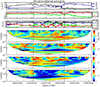 |
Fig. 1. Example of a helical structure (HS) observed by Solar Orbiter on April 27, 2021. From top to bottom: Total ion density and solar wind radial speed (VR) in black and blue, respectively; the transverse and normal component (VT and VN) of the solar wind speed; the Radial-Transverse-Normal (RTN) component of the interplanetary magnetic field along with |B|; the wavelet spectrum of the total ion density; spectrogram of the normalized reduced magnetic helicity, σm; spectrogram of the normalized cross helicity, σc; and spectrogram of the normalized residual energy, σr. The vertical black and the dashed horizontal white lines denote the PDS start and end time and the fPDS ± 0.15 mHz range, respectively. The black contour in the wavelet spectrum corresponds to the wavelet power threshold (see also Katsavrias et al. 2026 for more details). The black contour in the σm, σc, and σr panels corresponds to |σm| = 0.7. |
3. Results and discussion
Based on the analysis described in the previous section, we identified 751, 893, and 763 HS in 592, 738, and 607 PDS events for the window intervals of 6, 12, and 18 hours, respectively (black bars in the left panel of Fig. 2) because some PDS events contained more than one HS. The list is publicly available2. The percentage of PDSs containing an HS is 34.3, 33.8, and 32.1% for the window intervals of 6, 12, and 18 hours, respectively (black bars in the right panel of Fig. 2). In contrast, and as a test sample, the percentage of PDS events having HS ±2 hours outside the start and end time limits is 10, 5.7, and 5.3%. This indicates that HSs are a particular constituent of these < 1 mHz PDSs.
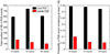 |
Fig. 2. Total number (left panel) and percentage (right panel) of PDS events containing at least one helical structure (HS) within (black bars) and outside (red bars) the PDS start and end time limits for the window intervals of 6, 12, and 18 hours, respectively. |
To obtain a collective view on the HS inside the PDS start and end time limits, we calculated and plotted for each HS the averaged σc and σr. Figure 3 shows the results for the window intervals of 6, 12, and 18 hours, with a further separation of the HSs based on the accompanied solar wind speed value. Most of the data lie in the bottom right quadrant of the unit-radius circle shown as a dashed black curve, as was observed before (e.g., Bavassano et al. 1998). Fast wind tends to be more Alfvénic, with large σc and small |σr|. Moreover, we identified three subcategories of HSs (color-shaded areas in Fig. 3) that we list below.
-
Following Zhao et al. (2020), HSs characterized by |σc|< 0.4 and σr < −0.5 (shaded green area) are candidate small flux ropes. A meaningful value of σc was obtained by first rectifying the magnetic field, so that positive σc was defined as the antisunward flux. As shown, most candidate small flux ropes (≈80% in all three window intervals) were observed during intervals with Vsw < 500 km/s. Nevertheless, the remaining ≈20% are observed in the fast solar wind as well, and this agrees with Chen & Hu (2025). We note that due to our criteria and method, we cannot rule out the possibility that other HS outside the shaded green area may be flux ropes. One example are structures with a low cross helicity and a low but still negative residual energy (|σc|< 0.4 and −0.5 < σr < 0), which may include flux ropes with a much smaller remaining plasma flow (Zhao et al. 2020).
-
Another example are Alfvén waves that coexist within a magnetic flux rope, which our method cannot distinguish from stand-alone Alfvén waves. Therefore, HSs characterized by |σc|> 0.5 and |σr|< 0.1 (shaded yellow areas) are categorized as Alfvénic HSs (Borovsky 2020). These HSs are observed almost equally often (≈50% in all three window intervals) during periods of the fast and slow solar wind, and their vast majority corresponds to forward-propagating Alfvén wave modes.
-
Finally, complex HSs characterized by |σc|> 0.4 and σr < −0.5 (shaded magenta areas). Although this category contains magnetically dominated HSs (σr < −0.5), it also exhibits significant Alfvénic activity. A possible explanation for this category might be that the flux rope remains tethered to the Sun, and the spacecraft crosses one of the flux rope legs instead of the core, as suggested for a magnetic flux rope in ICMEs (see also Fig. 6 in Good et al. 2022). This category might also include small-scale magnetic flux ropes exhibiting field-aligned flows. In particular, using Parker Solar Probe observations, Chen et al. (2021) and Chen & Hu (2022) recently showed that flux ropes can sometimes maintain their shape while also carrying significant plasma flow that is aligned with the local magnetic field. This configuration might be characterized by a high cross helicity and a wide range of residual energy, including magnetically dominated cases. On the other hand, and even though our dataset was filtered at f < 1 mHz, which corresponds to structures with scales larger than 5.5 minutes, we cannot exclude the possibility that larger-scale switchbacks are detected. These might correspond to the population in the area of σc ≈ 1 and negative σr (Bourouaine et al. 2020; Agapitov et al. 2022).
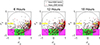 |
Fig. 3. Normalized residual energy (σr) vs. normalized cross helicity (σc) for all HSs with |σm|≥0.7 within the < 1 mHz PDS events in out list. The HSs are color-coded based on the average solar wind speed, with black and red circles corresponding to Vsw < 500 km/s and Vsw ≥ 500 km/s, respectively. The shaded green, yellow, and magenta areas represent the regions that likely contain flux ropes, Alfvénic HSs, and complex HSs, respectively. |
Moreover, we provided the observational locations in terms of solar ecliptic longitude versus heliocentric distance to facilitate comparisons with other inner heliosphere observations. As shown in the left panel of Fig. A.1, the PDS events and the embedded helical structures were identified across all Solar Orbiter locations, spanning a range of ≈0.3 to 1 AU.
In order to investigate the relative occurrence of each HS type in our sample, we calculated the probability of occurrence, with respect to the total HS number, for the various HS types detected within the PDS start and end time limits (left panel in Fig. 4). Similar to Fig. 2, we also showed the occurrence probability for the various HS types detected outside the PDS start and end time limits (right panel in Fig. 4). As shown, ≈30% of the HSs within the PDS start and end time limits (regardless of the window interval) have flux ropes properties (green bars). This means that at least 10% (≈30% of the flux ropes of ≈30% of the HS) of the < 1 mHz PDSs contain flux ropes (see also Fig. A.2). In contrast, flux ropes detected outside the PDS start and end time limits have an occurrence probability lower than 2%. Alfvénic HSs, on the other hand, exhibit a very different occurrence. The percentage of Alfvénic HSs observed within the PDS start and end time limits (yellow bars) is ≈10% of all HSs, which corresponds to ≈2−3% of the PDS events. Moreover, we identified ≈25−30% Alfvénic HSs outside the PDS start and end time limits, which also corresponds to ≈2−3% of the PDS events.
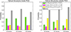 |
Fig. 4. Occurrence probability with respect to the total HS number for the various HS types detected inside (left panel) and outside (right panel) of the PDS start and end time limits. The HS are colored similarly to the shaded areas in Fig. 3, with green, magenta and yellow bars corresponding to flux ropes, complex events, and Alfvénic HSs, respectively. |
These results indicate that small flux ropes can be considered as constituents of PDSs, in contrast to Alfvénic HSs, which have the same occurrence probability within and outside of PDSs. The increase in the number of flux ropes observed inside PDSs indicates that PDS events are associated with reconnection. This result agrees with several previous theoretical (Endeve et al. 2005; Lynch et al. 2014; Réville et al. 2020; Peterson et al. 2021) and observational studies (Viall & Vourlidas 2015; Lavraud et al. 2020; Gershkovich et al. 2022) that associated f < 1 mHz PDSs with the reconnection processes. Especially observational studies have provided multiple lines of in situ evidence, including composition changes, temperature changes, and magnetic connectivity (strahl), that are consistent with magnetic reconnection as a source of PDSs. We provided observations of the embedded flux ropes themselves using a large statistical sample for the first time, to our knowledge.
We emphasize that the occurrence probability of flux ropes in PDSs (≈10%), although small in magnitude, is statistically important. As discussed before, our criteria and method impose limitations in that some of the HSs in other categories (e.g., Alfvénic HSs or complex HSs) might also be flux ropes; nevertheless, we have no way to distinguish between them. Furthermore, we focused on flux ropes with |σm|> 0.7 and |σc|< 0.4, which can be thought of as force-free structures. Nevertheless, flux ropes with a high cross helicity and |σm|< 0.7 have also been identified in the literature and can be thought of as the result of the combined attraction by a force-free solution (where the magnetic helicity is maximized and the cross helicity is zero) and an Alfvénic solution (Telloni et al. 2016). Furthermore, Higginson & Lynch (2018) used MHD simulation to show that reconnection-generated flux ropes were embedded between small density blobs (streamer blobs). Nevertheless, they argued that not each reconnection event that produces magnetic and density structures might result in a proper flux rope, which is also consistent with observational studies (Kepko et al. 2016; Di Matteo et al. 2019). Recently, Choi et al. (2024) also exploited the corotation of the Parker Solar Probe with the Sun near perihelion to identify a series of small flux ropes. The authors indicated that these series were consistent with the picture that flux ropes are embedded in between blobs, but not all of them were successfully fit to the force-free model.
The 139, 165, and 162 small flux ropes identified within the start and end time limits of PDS events using intervals of 6, 12, and 18 hours, respectively, are publicly available (Katsavrias & Di Matteo 2025b). The list is in excel format with different excel sheets for each analysis interval. For each flux rope, we provide the start and end time as determined by the wavelet analysis, together with the mean values of σm, σc, and σr. Supplementary information is also given as follows: the location of the spacecraft (radial distance in AU, and the longitude and latitude in solar ecliptic coordinates), the corresponding PDS frequency, the average solar wind speed, and the spacecraft speed.
Limitations also exist due to the dataset we used. Our dataset is limited to measurements close to the ecliptic plane during the rising phase and maximum of solar cycle 25. Since the solar activity can affect the properties of PDSs (Kepko et al. 2020), our results are valid only within the solar cycle phase we analyzed. Moreover, Cartwright & Moldwin (2010) argued that flux ropes that are indeed remnants of the streamer belt blobs would exhibit a reduced occurrence during solar maximum because the helmet streamers are less confined to the solar equator. Finally, and most importantly, we have no information about the proton and α particle density, since they were not publicly available at the time of this investigation. The contribution of protons is usually dominant in the total ion density, and we therefore expect no significant changes in our list of events (Di Matteo et al. 2024). However, the α/p ratio is a crucial parameter of PDSs when a solar origin is to be identified (Kepko et al. 2024). Coherent PDSs (a common periodic behavior in the proton density and α/p ratio) have been shown to exhibit properties that are very different from those of incoherent events. Katsavrias et al. (2024) studied an extensive list of f < 1 mHz PDS and found that only 28% of more than 1000 events exhibited high coherence and thermodynamic signatures of the flux ropes. Therefore, information on the PDS coherence could drastically increase the occurrence probability of flux ropes.
Finally, we performed a basic statistical investigation of the radial distribution of the observed HS. Figure 5 shows the occurrence probability with respect to the total HS number versus the heliocentric distance of the flux ropes and Alfvénic HSs detected within the PDS start and end time limits. As shown, the flux rope occurrence rate appears to increase with increasing radial distance, while Alfvénic HSs decrease. This agrees with the results shown in the right panel of Fig. A.1. This trend might support the hypothesis that some of these flux ropes, or similar signatures, are created in situ (Farooki et al. 2024), for example, by magnetic reconnection across the heliospheric current sheet (Moldwin et al. 2000) or by turbulence (Viall et al. 2021). The latter is also supported by the increase in flux ropes at the expense of Alfvénicity. These in situ created flux ropes might explain the origin of PDSs without a coronal composition signature, that is, without a common periodic behavior in proton density and α/p ratio. Even though this result is intriguing, further analysis is required. For example, we already discussed the limited extent of our dataset in time, covering only solar maximum, and in space, with 50% of the time spent above 0.86 AU. Additionally, our strict criteria might favor the identification of a flux rope/HS near L1 over those closer to the Sun. For example, small-scale flux ropes might not be fully evolved or be in pressure balance with their surroundings (compared to near L1). Several studies also suggested that flux ropes first form at small spatial scales and can then evolve into larger ones by merging as they propagate in the interplanetary medium (Choi et al. 2024). Moreover, they might present more complex properties during solar maximum than during solar minimum. A more extended dataset along with further information on the α/p ratio would help us to reduce these hurdles, and we plan to address this in the future when more data are available.
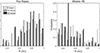 |
Fig. 5. Occurrence probability normalized with respect to the total HS number in each bin vs. the heliocentric distance of the flux ropes (left panel) and Alfvénic HSs (right panel) detected within the PDS start and end time limits. |
4. Summary and conclusions
Using 3.5 years of Solar Orbiter measurements that span the rising phase and maximum of solar cycle 25 (2021–2024), we have investigated the existence of embedded helical structures (|σm|> 0.7) in low-frequency (< 1 mHz) PDS events, identified at radial distances between 0.3 and 1 AU. We identified 751, 893, and 763 helical structures (HS) in 592, 738, and 607 PDS events for the window intervals of 6, 12, and 18 hours, respectively, which translates into 34.3, 33.8, and 32.1%. In contrast, the percentage of HSs detected in the vicinity of PDS was lower than 10% (for the three window intervals), indicating that HSs are a particular constituent of low-frequency PDS.
By further exploiting the normalized cross helicity and residual energy of the identified HSs, we classified them as small flux ropes (|σc|< 0.4 and σr < −0.5) or Alfvénic structures (|σc|> 0.5 and |σr|< 0.1). Our results indicate that small flux ropes are a particular constituent of PDS events, since the percentage of low frequency PDS that have embedded flux ropes was 10% at least (for the three window intervals), while flux ropes detected in the vicinity of the PDS (outside the PDS start and end time limits) exhibited an occurrence probability lower than 2%. In contrast, Alfvénic HSs exhibited a similar occurrence probability (2−3%) within and outside the PDS. This is an important addition to the scenario in which PDSs are formed by processes involving magnetic reconnection in either the solar corona or en route.
However, these statistical results include limitations due to the dataset we used. A more detailed analysis, including α/p ratio information (not currently available), can provide a more reliable picture of the percentage of flux ropes that are embedded in PDSs of pure solar origin. Furthermore, the combined use of Solar Orbiter and Parker Solar Probe (or similar missions) can provide a more extensive spatio-temporal coverage, also including various solar cycle phases, which might affect the detection of these small flux ropes.
Acknowledgments
This material is based upon work supported by the National Aeronautics and Space Administration through the completed Heliophysics Internal Scientist Funding Model Program. The authors thank the Solar Orbiter team for the use permission of the data and the ESA Solar Orbiter archive for making these data available (https://soar.esac.esa.int/soar/). CK received support from the ESA Archival Research Visitor Programme. S.D. was also supported by NASA Grant 80NSSC21K0459. The PDS list is publicly available at https://zenodo.org/records/16038091 and the flux rope list at https://zenodo.org/records/16992925.
References
- Agapitov, O. V., Drake, J. F., Swisdak, M., et al. 2022, ApJ, 925, 213 [NASA ADS] [CrossRef] [Google Scholar]
- Allred, J. C., & MacNeice, P. J. 2015, Comput. Sci. Discov., 8, 015002 [Google Scholar]
- Alzate, N., Di Matteo, S., Morgan, H., Viall, N., & Vourlidas, A. 2024, ApJ, 973, 130 [Google Scholar]
- Antiochos, S. K., Mikić, Z., Titov, V. S., Lionello, R., & Linker, J. A. 2011, ApJ, 731, 112 [Google Scholar]
- Bavassano, B., Pietropaolo, E., & Bruno, R. 1998, J. Geophys. Res., 103, 6521 [NASA ADS] [CrossRef] [Google Scholar]
- Borovsky, J. E. 2020, J. Geophys. Res., 125, e27377 [Google Scholar]
- Borovsky, J. E., & Denton, M. H. 2006, J. Geophys. Res.: Space Phys., 111, A07S08 [Google Scholar]
- Bourouaine, S., Perez, J. C., Klein, K. G., et al. 2020, ApJ, 904, L30 [Google Scholar]
- Bruno, R., & Carbone, V. 2013, Liv. Rev. Sol. Phys., 10, 2 [Google Scholar]
- Cartwright, M. L., & Moldwin, M. B. 2010, J. Geophys. Res., 115, A08102 [Google Scholar]
- Chen, Y., & Hu, Q. 2022, ApJ, 924, 43 [NASA ADS] [CrossRef] [Google Scholar]
- Chen, Y., & Hu, Q. 2025, J. Geophys. Res., 130, 2024JA033130 [Google Scholar]
- Chen, Y., Hu, Q., Zhao, L., Kasper, J. C., & Huang, J. 2021, ApJ, 914, 108 [NASA ADS] [CrossRef] [Google Scholar]
- Choi, K.-E., Lee, D.-Y., Noh, S.-J., & Agapitov, O. 2024, ApJ, 961, 3 [Google Scholar]
- DeForest, C. E., Howard, R. A., Velli, M., Viall, N., & Vourlidas, A. 2018, ApJ, 862, 18 [Google Scholar]
- Di Matteo, S., Viall, N. M., Kepko, L., et al. 2019, J. Geophys. Res., 124, 837 [NASA ADS] [CrossRef] [Google Scholar]
- Di Matteo, S., Villante, U., Viall, N., Kepko, L., & Wallace, S. 2022, J. Geophys. Res., 127, e2021JA030144 [Google Scholar]
- Di Matteo, S., Katsavrias, C., Kepko, L., & Viall, N. M. 2024, ApJ, 969, 67 [Google Scholar]
- Endeve, E., Lie-Svendsen, O., Hansteen, V. H., & Leer, E. 2005, ApJ, 624, 402 [NASA ADS] [CrossRef] [Google Scholar]
- Farooki, H., Noh, S. J., Lee, J., et al. 2024, ApJS, 271, 42 [Google Scholar]
- Gershkovich, I., Lepri, S. T., Viall, N. M., Di Matteo, S., & Kepko, L. 2022, ApJ, 933, 198 [NASA ADS] [CrossRef] [Google Scholar]
- Good, S. W., Hatakka, L. M., Ala-Lahti, M., et al. 2022, MNRAS, 514, 2425 [NASA ADS] [CrossRef] [Google Scholar]
- Higginson, A. K., & Lynch, B. J. 2018, ApJ, 859, 6 [Google Scholar]
- Horbury, T. S., O’Brien, H., Carrasco Blazquez, I., et al. 2020, A&A, 642, A9 [NASA ADS] [CrossRef] [EDP Sciences] [Google Scholar]
- Katsavrias, C., & Di Matteo, S. 2025a, https://doi.org/10.5281/zenodo.16038091 [Google Scholar]
- Katsavrias, C., & Di Matteo, S. 2025b, https://doi.org/10.5281/zenodo.16992925 [Google Scholar]
- Katsavrias, C., Preka-Papadema, P., & Moussas, X. 2012, Sol. Phys., 280, 623 [CrossRef] [Google Scholar]
- Katsavrias, C., Papadimitriou, C., Hillaris, A., & Balasis, G. 2022, Atmosphere, 13, 499 [NASA ADS] [CrossRef] [Google Scholar]
- Katsavrias, C., Nicolaou, G., Di Matteo, S., et al. 2024, A&A, 686, L10 [NASA ADS] [CrossRef] [EDP Sciences] [Google Scholar]
- Katsavrias, C., Di Matteo, S., Kepko, L., Viall, N., & Walsh, A. 2026, Sol. Phys., 301 [Google Scholar]
- Kepko, L., Viall, N. M., Antiochos, S. K., et al. 2016, Geophys. Res. Lett., 43, 4089 [NASA ADS] [CrossRef] [Google Scholar]
- Kepko, L., Viall, N. M., & Wolfinger, K. 2020, J. Geophys. Res., 125, e28037 [NASA ADS] [CrossRef] [Google Scholar]
- Kepko, L., Viall, N. M., & DiMatteo, S. 2024, J. Geophys. Res.: Space Phys., 129, e2023JA031403 [Google Scholar]
- Kurien, L. V., Kanekal, S. G., Di Matteo, S., et al. 2024, J. Geophys. Res.: Space Phys., 129, e2024JA032614 [Google Scholar]
- Lavraud, B., Fargette, N., Réville, V., et al. 2020, ApJ, 894, L19 [Google Scholar]
- Lynch, B. J., Edmondson, J. K., & Li, Y. 2014, Sol. Phys., 289, 3043 [Google Scholar]
- Matthaeus, W. H., Goldstein, M. L., & Smith, C. 1982, Phys. Rev. Lett., 48, 1256 [Google Scholar]
- Moldwin, M. B., Ford, S., Lepping, R., Slavin, J., & Szabo, A. 2000, Geophys. Res. Lett., 27, 57 [NASA ADS] [CrossRef] [Google Scholar]
- Morlet, J., Arens, G., Fourgeau, E., & Giard, D. 1982, Geophysics, 47, 222 [NASA ADS] [CrossRef] [Google Scholar]
- Owen, C. J., Bruno, R., Livi, S., et al. 2020, A&A, 642, A16 [EDP Sciences] [Google Scholar]
- Peterson, E. E., Endrizzi, D. A., Clark, M., et al. 2021, J. Plasma Phys., 87, 905870410 [NASA ADS] [CrossRef] [Google Scholar]
- Poirier, N., Réville, V., Rouillard, A. P., Kouloumvakos, A., & Valette, E. 2023, A&A, 677, A108 [NASA ADS] [CrossRef] [EDP Sciences] [Google Scholar]
- Réville, V., Velli, M., Rouillard, A. P., et al. 2020, ApJ, 895, L20 [Google Scholar]
- Sanchez-Diaz, E., Rouillard, A. P., Davies, J. A., et al. 2017, ApJ, 851, 32 [Google Scholar]
- Schlenker, M. J., Antiochos, S. K., MacNeice, P. J., & Mason, E. I. 2021, ApJ, 916, 115 [Google Scholar]
- Telloni, D., Bruno, R., D’Amicis, R., Pietropaolo, E., & Carbone, V. 2012, ApJ, 751, 19 [Google Scholar]
- Telloni, D., Carbone, V., Perri, S., et al. 2016, ApJ, 826, 205 [Google Scholar]
- Torrence, C., & Compo, G. P. 1998, Bull. Am. Meteorol. Soc., 79, 61 [Google Scholar]
- Ventura, R., Antonucci, E., Downs, C., et al. 2023, A&A, 675, A170 [NASA ADS] [CrossRef] [EDP Sciences] [Google Scholar]
- Viall, N. M., & Vourlidas, A. 2015, ApJ, 807, 176 [Google Scholar]
- Viall, N. M., Kepko, L., & Spence, H. E. 2009, J. Geophys. Res., 114, A01201 [Google Scholar]
- Viall, N. M., DeForest, C. E., & Kepko, L. 2021, Front. Astron. Space Sci., 8, 139 [NASA ADS] [CrossRef] [Google Scholar]
- Zhao, L.-L., Zank, G. P., Adhikari, L., et al. 2020, ApJS, 246, 26 [Google Scholar]
Appendix A: Supplementary figures
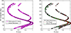 |
Fig. A.1. Observational locations of the PDS events and the embedded helical structures (HS), flux ropes and Alfvénic HS identified in Solar Orbiter data. Left panel: Observational locations of < 1 mHz PDS and helical structures (|σm|> 0.7) with magenta stars and black dots, respectively. Right panel: Observational locations of helical structures (|σm|> 0.7), flux ropes and Alfvénic HS with black stars, red and green dots, respectively. |
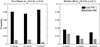 |
Fig. A.2. Probability of occurrence, with respect to the total PDS number, for the flux ropes (left panel) and Alfvénic helical structures (right panel), respectively. Helical structure (HS) types detected inside and outside of the PDS start and end time limits are shown with black and grey bars, respectively. |
All Figures
|
Fig. 1. Example of a helical structure (HS) observed by Solar Orbiter on April 27, 2021. From top to bottom: Total ion density and solar wind radial speed (VR) in black and blue, respectively; the transverse and normal component (VT and VN) of the solar wind speed; the Radial-Transverse-Normal (RTN) component of the interplanetary magnetic field along with |B|; the wavelet spectrum of the total ion density; spectrogram of the normalized reduced magnetic helicity, σm; spectrogram of the normalized cross helicity, σc; and spectrogram of the normalized residual energy, σr. The vertical black and the dashed horizontal white lines denote the PDS start and end time and the fPDS ± 0.15 mHz range, respectively. The black contour in the wavelet spectrum corresponds to the wavelet power threshold (see also Katsavrias et al. 2026 for more details). The black contour in the σm, σc, and σr panels corresponds to |σm| = 0.7. |
| In the text | |
|
Fig. 2. Total number (left panel) and percentage (right panel) of PDS events containing at least one helical structure (HS) within (black bars) and outside (red bars) the PDS start and end time limits for the window intervals of 6, 12, and 18 hours, respectively. |
| In the text | |
|
Fig. 3. Normalized residual energy (σr) vs. normalized cross helicity (σc) for all HSs with |σm|≥0.7 within the < 1 mHz PDS events in out list. The HSs are color-coded based on the average solar wind speed, with black and red circles corresponding to Vsw < 500 km/s and Vsw ≥ 500 km/s, respectively. The shaded green, yellow, and magenta areas represent the regions that likely contain flux ropes, Alfvénic HSs, and complex HSs, respectively. |
| In the text | |
|
Fig. 4. Occurrence probability with respect to the total HS number for the various HS types detected inside (left panel) and outside (right panel) of the PDS start and end time limits. The HS are colored similarly to the shaded areas in Fig. 3, with green, magenta and yellow bars corresponding to flux ropes, complex events, and Alfvénic HSs, respectively. |
| In the text | |
|
Fig. 5. Occurrence probability normalized with respect to the total HS number in each bin vs. the heliocentric distance of the flux ropes (left panel) and Alfvénic HSs (right panel) detected within the PDS start and end time limits. |
| In the text | |
|
Fig. A.1. Observational locations of the PDS events and the embedded helical structures (HS), flux ropes and Alfvénic HS identified in Solar Orbiter data. Left panel: Observational locations of < 1 mHz PDS and helical structures (|σm|> 0.7) with magenta stars and black dots, respectively. Right panel: Observational locations of helical structures (|σm|> 0.7), flux ropes and Alfvénic HS with black stars, red and green dots, respectively. |
| In the text | |
|
Fig. A.2. Probability of occurrence, with respect to the total PDS number, for the flux ropes (left panel) and Alfvénic helical structures (right panel), respectively. Helical structure (HS) types detected inside and outside of the PDS start and end time limits are shown with black and grey bars, respectively. |
| In the text | |
Current usage metrics show cumulative count of Article Views (full-text article views including HTML views, PDF and ePub downloads, according to the available data) and Abstracts Views on Vision4Press platform.
Data correspond to usage on the plateform after 2015. The current usage metrics is available 48-96 hours after online publication and is updated daily on week days.
Initial download of the metrics may take a while.