| Issue |
A&A
Volume 709, May 2026
|
|
|---|---|---|
| Article Number | A89 | |
| Number of page(s) | 16 | |
| Section | Extragalactic astronomy | |
| DOI | https://doi.org/10.1051/0004-6361/202557764 | |
| Published online | 05 May 2026 | |
The twin-jet system in the Fanaroff-Riley II radio galaxy 3C 452
A sub-parsec-scale VLBI study
1
Max-Planck-Institut für Radioastronomie, Auf dem Hügel 69, D-53121 Bonn, Germany
2
Leiden Observatory, Leiden University, PO Box 9513, 2300 RA, Leiden, The Netherlands
3
Julius-Maximilians-Universität Würzburg, Fakultät für Physik und Astronomie, Institut für Theoretische Physik und Astrophysik, Lehrstuhl für Astronomie, Emil-Fischer-Str. 31, D-97074 Würzburg, Germany
4
INAF – Osservatorio di Astrofisica e Scienza dello Spazio di Bologna, Via Gobetti 101, 40129 Bologna, Italy
5
INAF–Istituto di Radioastronomia, Bologna, Via Gobetti 101, 40129 Bologna, Italy
6
Dipartimento di Fisica e Astronomia, Università degli Studi di Bologna, Via Gobetti 93/2, 40129 Bologna, Italy
★ Corresponding author: This email address is being protected from spambots. You need JavaScript enabled to view it.
Received:
20
October
2025
Accepted:
25
February
2026
Abstract
Aims. We present a comprehensive multifrequency VLBI analysis of the Fanaroff-Riley II (FRII) high-excitation radio galaxy 3C 452. Our aim is to resolve and analyze, for the first time, its twin-jet structure on sub-parsec scales.
Methods. Our dataset comprises high-sensitivity array (HSA) observations at 4.9, 8.4, 15.4, 23.6, and 43.2 GHz. Through fitting methods performed in both the visibility and the image plane, we were able to trace the jet expansion from scales of a few thousand to nearly 105 Schwarzschild radii (RS) for both the approaching and receding jets. Additionally, we derived the core brightness temperatures and Doppler factors to constrain the orientation and intrinsic speed of the jet.
Results. Our study provides the first detailed description of the twin-jet system in 3C 452 on VLBI scales, confirming it as a rare FRII source with jets detected down to millimeter wavelengths. We resolved both the jet and counter-jet down to scales of a few thousand RS, revealing a symmetric parabolically expanding structure with power-law indices of k ≈ 0.66 (jet) and k ≈ 0.47 (counter-jet). Jet-to-counter-jet intensity ratios remain nearly constant on larger scales but rise sharply within the inner 1−1.5 mas, as revealed by the higher-frequency data, consistent with increasing jet speed. We observed low core brightness temperatures, which are indicative of Doppler de-boosting (δ ∼ 0.03 − 0.83) due to the large viewing angle (θ ≈ 70°) and/or a magnetically dominated jet base. A spectral index analysis revealed a strongly inverted core spectrum (α > 2) with additional absorption at the highest frequencies, followed by a sharp steepening (α ∼ −2.5) to optically thin values in the innermost jet. Finally, a comparison between broad- and narrow-line high-excitation radio galaxies showed that jets in narrow-line sources, such as 3C 452 and Cygnus A, complete collimation at ≲105 RS, whereas broad-line sources exhibit shape transitions at 106 − 107 RS, suggesting that orientation plays an important role in the observed collimation scales.
Key words: instrumentation: high angular resolution / galaxies: active / galaxies: individual: 3C 452 / galaxies: jets
© The Authors 2026
 Open Access article, published by EDP Sciences, under the terms of the Creative Commons Attribution License (https://creativecommons.org/licenses/by/4.0), which permits unrestricted use, distribution, and reproduction in any medium, provided the original work is properly cited.
This article is published in open access under the Subscribe to Open model.
Open access funding provided by Max Planck Society.
1. Introduction
Extragalactic jets are collimated outflows of relativistic plasma powered by the accretion of material onto a supermassive black hole at the center of active galactic nuclei (AGNs) (see, e.g., Blandford et al. 2019). High-frequency very long-baseline interferometry (VLBI) observations represent a unique tool to unveil the fundamental processes that drive their formation (see Boccardi et al. 2017, and references therein). Most VLBI studies of AGN jets have focused on blazars, while radio galaxies offer a unique advantage in such studies because projection effects and Doppler boosting play a minor role compared to blazars. In particular, studies of nearby radio galaxies with jets oriented at a large viewing angle can be highly informative because they allow us to probe the intrinsic jet properties in the immediate vicinity of the black hole.
Radio galaxies known to be bright enough to probe the jet sub-parsec scales down to millimeter wavelengths are rare, especially among the class of powerful high-excitation galaxies (HEGs) (Boccardi et al. 2025). These sources are thought to be powered by radiatively efficient cold accretion disks fed by cold gas (Heckman & Best 2014), and they typically produce powerful jets that develop Fanaroff-Riley II (FRII) morphologies (Fanaroff & Riley 1974) on kiloparsec scales. Even rarer are HEGs showing sufficiently bright two-sided jets on such small scales, a property that enables important tests of the jet symmetry to be performed. The two-sided FRII jet in Cygnus A is currently the only case in which such millimeter-VLBI studies could be carried out (Boccardi et al. 2016). With the aim of identifying new targets for jet formation studies, including HEGs, Boccardi et al. (2025) carried out a VLBI experiment using the High Sensitivity Array (HSA) at 22 GHz (1 cm) and 43 GHz (7 mm) and considering 16 radio galaxies poorly explored on VLBI scales. These sources were selected among those characterized by a high spatial resolution in units of Schwarzschild radii, which results from their proximity (z < 0.1) and large black hole mass (log MBH > 8.5).
Among the HEGs in this sample, the radio galaxy 3C 452 emerged as the most interesting target. This source is located at redshift z = 0.081 and hosts a black hole with mass MBH = ∼8 × 10⁸ M⊙ (Koss et al. 2022). The existence of a radiatively efficient accretion disk at the center of this object has been indicated by optical spectroscopic studies (e.g., Buttiglione et al. 2010), which also classify 3C 452 as an HEG based on the excitation index parameter1. The lack of broad emission lines, that is, the source classification as a narrow-line radio galaxy (e.g., Véron-Cetty & Véron 2006), implies obscuration of the nuclear regions due to the presence of a compact absorber, as confirmed by X-ray observations (Fioretti et al. 2013). In large-scale radio observations performed with the Very Large Array (VLA), 3C 452 exhibits a symmetric double morphology (e.g., Black et al. 1992). Its largest angular size of ∼5 arcmin in 1.4 GHz maps corresponds to a projected linear size of ∼450 kpc at the source redshift of z = 0.081 (e.g., Shelton et al. 2011). In addition, low-frequency observations have revealed the presence of megaparsec-scale relic radio lobes associated with this source (Sirothia et al. 2013). The source was previously almost unexplored on VLBI scales. A single image at 5 GHz was presented by Giovannini et al. (2001). This revealed a highly symmetric two-sided structure with a total flux density of ∼130 mJy. Taking into account the core dominance and jet symmetry, the authors constrained the jet to be oriented at an angle of θ ≥ 60° with respect to the line of sight. The 22 GHz and 43 GHz observations by Boccardi et al. (2025) detected a twin-jet structure down to the sub-parsec scales. At these high frequencies, 3C 452 was shown to be still relatively bright, with a total flux density of ∼68 mJy at 22 GHz and ∼53 mJy at 43 GHz. Therefore, follow-up VLBI observations were requested with the aim of addressing several open questions concerning the jet launching regions in powerful sources.
In this article, we present VLBI observations of 3C 452 at frequencies between 5 GHz and 43 GHz. The aim of this work is to obtain a first description of the fundamental parameters of this jet on sub-parsec scales (i.e., orientation and Doppler factor) and to investigate whether the physical processes of jet acceleration and collimation are still taking place on the examined scales. At the source redshift (z = 0.0811) and assuming a Λ cold dark matter cosmology (ΛCDM) with H0 = 71 km s−1 Mpc−1, ΩM = 0.27, and ΩΛ = 0.73, an angular scale of 1 mas corresponds to ≈1.508 pc. Given a black hole mass of 8 × 10⁸ M⊙, this translates to ≈19 738 Schwarzschild radii (RS) per mas. Thus, these observations provide an angular resolution down to a few thousand RS, which is sufficient to resolve the jet base at a close distance from the central engine.
The paper is structured as follows. In Sect. 2, we present the multifrequency VLBI observations, describe the data reduction process, and outline the analysis methods, including model fitting, image alignment across frequencies, and the construction of stacked maps. The results and their interpretation are presented in Sect. 3, covering the flux density and jet-to-counter-jet profiles, the core brightness temperatures, the jet collimation properties, and the spectral index distribution along the ridge line. A comparison with Cygnus A and other HEGs is presented in Sect. 4. We summarize our conclusions in Sect. 5.
2. Dataset and analysis
On 2 January 2022, we conducted HSA observations using the Very Long Baseline Array (VLBA) and the Effelsberg 100-m radio telescope (Project code: BM516A). The inclusion of Effelsberg improved the angular resolution and sensitivity, necessary for a detailed imaging of the sub-parsec-scale structures in our faint target. The observations spanned a 12-hour block for optimal (u, v)-coverage. Data were collected at five frequencies: 4.9 GHz, 8.4 GHz, 15.4 GHz, 23.6 GHz, and 43.2 GHz. A 4 Gbit/s recording mode was used in the experiment. The observations employed ten VLBA antennas, recording in both polarizations with 256 spectral channels per baseband and a total bandwidth of 128 MHz. The data were correlated using the DiFX software correlator in Socorro with an integration time of 2 seconds. The total on-source times for 3C 452 were 0.800 hours at 4.9 GHz, 1.000 hours at 8.3 GHz, 1.600 hours at 15.3 GHz, 2.092 hours at 23.6 GHz, and 3.867 hours at 43.2 GHz. However, at 43.2 GHz, the experiment was affected by severe problems. An error in the correction of azimuth and elevation offsets affected the 7 mm performance of the VLBA antennas, resulting in a ∼40% sensitivity loss and a change in the flux density scale. Effelsberg also malfunctioned at 7 mm. This prevented us from imaging the source at the highest frequency. Consequently, we requested and obtained time to repeat the experiment at all five frequencies (Project code: BM516B). In these observations, which were carried out on 6 August 2022, the Kitt Peak antenna did not participate due to ongoing power issues after a wildfire. Nevertheless, in this epoch we were able to image the source at all bands. These data were calibrated using the Astronomical Image Processing System (AIPS, Greisen 1990) following standard procedures, including an opacity correction at frequencies ≥15 GHz. The imaging and self-calibration of the amplitude and phase were performed in DIFMAP (Difference Mapping, Shepherd 1997). The log of observations and the characteristics of the clean images for both epochs are presented in Table 1. The images are presented in Appendix A. An overview of the structure of the source from the kiloparsec scale to the sub-parsec scale is shown in Fig. 1, including the VLA 1.4 GHz from the 3CRR Atlas (Leahy et al. 1996) and our natural weighted VLBI images from the project code BM516B at 4.9−43.2 GHz. In Fig. 1, we note a misalignment between the sub-parsec and kiloparsec jet position angles.
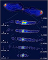 |
Fig. 1. Twin-jet structure of 3C 452 from kiloparsec to sub-parsec scales. The top image was obtained from VLA data at 1.4 GHz (Leahy et al. 1996). The following maps show the VLBI structure at different frequencies (4.9 GHz, 8.4 GHz, 15.4 GHz, 23.6 GHz, 43.2 GHz) based on the analyzed data of our project code BM516B presented in Sect. 2. Images were produced using natural weighting. The maps have been aligned to the central brightest feature. The complete series of images considered in the article is presented in the Appendix A. |
Log of observations and characteristics of the clean maps forming the multifrequency dataset.
Such misalignments are common in AGNs and may arise from a combination of intrinsic and environmental effects. Jet reorientation can occur when the accretion disk is misaligned with the black hole spin axis, inducing relativistic frame-dragging effects such as Lense–Thirring precession and the associated Bardeen–Petterson warp. These processes can lead to episodic changes in the jet launching direction, particularly if the fueling geometry varies with time. In close binary black hole systems, orbital motion and geodetic precession provide an alternative mechanism that can produce megayear-scale changes in jet orientation, comparable to those inferred from parsec-to-kiloparsec misalignments (e.g., Krause et al. 2019). Environmental interactions with the interstellar medium or the intragalactic medium, as well as jet backflow, may also contribute to the observed jet morphology, especially in radio galaxies, whereas parsec-scale misalignments have been discussed primarily in the context of quasars and BL Lacertae objects (e.g., Kharb et al. 2010).
2.1. Model fitting
With the aim of reconstructing the two-sided jet expansion profile and estimating the core brightness temperature, Tb, at all frequencies, we modeled the data using the MODELFIT subroutine in DIFMAP by fitting circular Gaussian components to the visibilities, which allowed us to determine, for each feature, the integrated flux density (S), the radial distance (r), the position angle (pa), and the size (d), corresponding to the full width at half maximum (FWHM) of the Gaussian.
The derived MODELFIT component parameters are reported for both projects, BM516A and BM516B, in Tables A.1 and A.2 in Appendix A. The radial distance of each feature, reported in column 3 of these tables, is relative to the position of the most compact component at the jet base, which was set as the origin in each map. The uncertainties for these parameters were estimated following the approach of Lee et al. (2008) based on the signal-to-noise ratio (S/N) of each emission feature. The S/N also defines the resolution limit of each component, which we considered when estimating the brightness temperature of the VLBI cores (Table A.3).
2.2. Alignment of maps at different frequencies
To meaningfully combine the data across all frequencies, it was essential to refer the measured radial distances of all jet components to a common origin, ideally corresponding to the central supermassive black hole. In each individual VLBI map, the origin coincides with the position of the peak emission, which is frequency dependent due to synchrotron opacity effects at the jet base (Blandford & Königl 1979; Lobanov 1998). To correct for this frequency-dependent shift, we performed a 2D cross-correlation analysis using optically thin regions of the jet in each frequency pair (see also Paraschos et al. 2021). We performed the cross-correlation using images produced with natural weighting to increase the sensitivity for the optically thin regions in the extended jet. For each pair of frequencies, the images were restored with a circular beam whose size corresponds to the arithmetic mean of the equivalent circular beams at the two frequencies. The pixel size was chosen to be one-tenth of the beam’s FWHM. In 3C 452, we found the spectral index distribution in the nuclear region, especially at the highest frequencies, to be very sensitive to the precision of the alignment. Therefore, we adopted a smaller pixel size and the mean beam in order to preserve sufficient resolution in the cross-correlation. Each map was first slightly shifted so that the pixel with the peak flux density was centered at the origin, introducing an inherent uncertainty corresponding to one pixel in both axes. After cross-correlation, we estimated the error in the derived shifts as the quadrature sum of the uncertainty of one pixel from the initial alignment and the one-pixel uncertainty of the correlation itself, following the method by Boccardi et al. (2021). The results of the cross-correlation, including the correlation coefficients and uncertainties, are presented in Table 2.
Results of the 2D cross-correlation for core shift determination.
After applying the derived core shifts, we recalculated the radial distances of all MODELFIT components using as the reference origin the most compact region of the two-sided jet base observed at 43 GHz, identified as the midpoint between the jet and counter-jet cores at that frequency. All images were then shifted to this common reference frame.
The selection of the reference position is further supported by the spectral index distribution along the jet ridge line (Fig. 8), which shows a maximum of α ≈ +3.2 near the same location, with S(ν)∝να. This is consistent with the expectation for a synchrotron self-absorbed core region, likely marking the position of the supermassive black hole. We restrict our discussion here to this validation aspect of the spectral index profile. A more detailed analysis of its spatial variation is presented in Sect. 3.5.
2.3. Stacked images analysis
The stacked images at 4.9 GHz, 8.4 GHz, 15.4 GHz, 23.6 GHz, and 43.2 GHz were restored with circular beams of 1.48 mas, 0.8 mas, 0.45 mas, 0.34 mas, and 0.18 mas, respectively. These beam sizes correspond to the average equivalent beams across the observing epochs. The stacked images at 22 GHz and 43 GHz were produced by combining data from our BM516A and BM516B observations with the 2018 observations from project BB393 (Boccardi et al. 2025). Alignment of the images was performed based on the position of the peak intensity in each epoch. The pixel size for each stacked image was set to one-fifth of the beam size. We used uniform weighting images for stacking to better define the transverse structure of the jet and allow for precise measurements of width and opening angle. The stacked images are shown in Fig. 2.
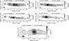 |
Fig. 2. Stacked VLBI images of 3C 452 at 4.9 (upper left), 8.4 (upper right), 15.4 (middle left), 23.6 (middle right), and 43.2 (bottom) GHz. The images were restored with circular beams of 1.48, 0.8, 0.45, 0.34, and 0.18 mas, respectively. The respective peak flux density and rms values are displayed at the top of each panel. The maps were produced using uniform weighting. |
We performed a pixel-based analysis of the stacked maps using the Python script presented by Ricci et al. (2022). The script requires input maps that are aligned along the y-axis and restored with a circular beam. The analysis divides the jet and counter-jet into one-pixel-wide slices oriented perpendicular to the jet’s direction. The flux density profile within each slice is then fit with a single 1D Gaussian function using the Levenberg-Marquardt algorithm (LevMarLSQFitter from the Astropy library). To minimize background noise contamination at the edges of the jet, pixels with values below 3σrms were excluded. The fitting process ends when the brightest pixel in the slice has an intensity lower than 5σrms.
The flux density in each slice was calculated by integrating the fitted Gaussian profile. The integrated flux and the FWHM of the Gaussian profiles were recorded and utilized to compute the flux density profiles, the jet opening angle as functions of the distance from the core, and the collimation profiles.
3. Results
3.1. Flux density profiles
The flux density profiles of the approaching jet and receding counter-jet in 3C 452, derived from the pixel-based analysis of the stacked VLBI images at all observed frequencies, are presented in Fig. 3. Both sides show a complex behavior with no clear symmetry in flux density between the jet and counter-jet.
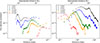 |
Fig. 3. Flux density profiles of the receding counter-jet (left panel) and approaching jet (right panel) and as a function of distance from the common reference frame, measured from the stacked images at each frequency. The profiles were derived using pixel-based Gaussian fitting across transverse jet slices, as described in Sect. 2.3. |
The approaching jet generally displays a decline in flux density with increasing distance from the core, consistent with synchrotron cooling and adiabatic expansion of the relativistic plasma. The decline is more pronounced in the inner few milliarcseconds, particularly at higher frequencies, and becomes less steep further downstream.
In contrast, the counter-jet profiles exhibit a more gradual evolution, with a slower decline compared to the approaching jet. This trend is especially evident at lower frequencies. The systematically lower brightness of the counter-jet across all bands may be primarily due to mild relativistic de-boosting, as expected given the inferred large viewing angle (Sect. 3.3). However, absorption effects could also play a role, particularly in the innermost regions. Given the source’s classification as a narrow-line radio galaxy and the presence of nuclear obscuration inferred from X-ray observations (Fioretti et al. 2013), both free-free absorption by a circumnuclear torus or dense ionized gas and synchrotron self-absorption in the counter-jet may contribute to the observed brightness asymmetry. In general, while both the jet and counter-jet show flux density gradients, the profiles are not symmetric, differing in both morphology and slope.
3.2. Jet-to-counter-jet intensity ratio
The jet-to-counter-jet intensity ratios (Rj/cj) were computed after applying the frequency-dependent core shifts listed in Table 2 and aligning all images to the most compact region in the 43.2 GHz map, as discussed in Sect. 2.2. Fig. 4 displays the frequency dependence of Rj/cj for three observing epochs. Here, Rj/cj was derived by summing the integrate flux densities of the MODELFIT components on each side after shifting the jet and counter-jet components to a common reference frame. The total jet flux density was then divided by the total counter-jet flux density at each frequency. Across most epochs and frequencies, the ratio remains relatively stable at ∼6.5. We observed an exception at 43.2 GHz in the BM516B epoch, where Rj/cj increases significantly. To further assess this deviation, we note that the 43.2 GHz core component reported by Boccardi et al. (2025) has a flux density of 28.50 ± 2.27 mJy when the source was likely in a quiescent state, whereas in our BM516B epoch, it is 42.25 ± 2.97 mJy, indicating a real increase in core emission. This increase in core flux density explains the elevated jet-to-counter-jet ratio at this frequency. This outlier is likely related to a transient flaring event in the approaching jet, where newly ejected material temporarily increases the observed ratio. Such events are expected to produce time-dependent brightness asymmetries, as the radiation from the counter-jet side travels a longer path to reach the observer and may not yet reflect the same ejection.
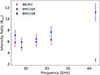 |
Fig. 4. Jet-to-counter-jet intensity ratio as a function of frequency. Ratios are derived for three datasets: BB393, BM516A, and BM516B. All images were aligned to the common reference frame, identified as the midpoint between the jet and counter-jet cores in the 43 GHz map (Sect. 2.2). The BB393 observations were published in Boccardi et al. (2025). |
Furthermore, the stability of Rj/cj at lower frequencies suggests that on larger scales, the emission is less affected by nuclear variability and opacity effects, which dominate closer to the core. This allows the jet and counter-jet to appear more comparable in brightness, even though their detailed flux density profiles remain distinct.
To further examine the spatial variation of the intensity, Fig. 5 plots the jet-to-counter-jet intensity ratio (Rj/cj) as a function of the projected distance along the jet, up to 5 mas (< 1.05 × 10⁵ RS). We focused on this scale because it is where the jet acceleration and collimation are expected (Boccardi et al. 2021). A clear trend emerged in the inner 1−1.5 mas (< 3 × 10⁴ RS), where the ratio exhibits a sharp rise, particularly at higher frequencies (22−43 GHz), reaching values up to ∼11. This sharp increase likely reflects an increasing jet speed. Beyond 1.5−2 mas, the ratio fluctuates moderately in the range of 5−8 at lower frequencies (5−15 GHz). This suggests that the jet is moving at a roughly constant speed in this region.
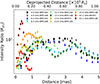 |
Fig. 5. Jet-to-counter-jet intensity ratio as a function of distance from the common reference frame, shown for all observing frequencies. The analysis includes data from projects BB393, BM516A, and BM516B. |
3.3. Core brightness temperature and jet orientation
For a nonthermal source, the apparent brightness temperature can be calculated using the following expression (e.g., Kadler et al. 2004):
 (1)
(1)
where Sν represents the flux density, ν is the frequency, and d denotes the diameter of the emitting region. From the MODELFIT analysis of our multifrequency data, we derived the brightness temperature of the core component. The uncertainties in the apparent brightness temperature were calculated by propagating the errors associated with the different parameters described in Sect. 2.1. All core component properties and resolution limits used for the TB estimates are reported in Table A.3 in the Appendix A. At 23.6 GHz, in the BM516A dataset, the core size was found to be smaller than the resolution limit. Therefore, we estimated only a lower limit for the brightness temperature by assuming a core size equal to the resolution limit.
In order to estimate the jet Doppler factor, we made an assumption on the intrinsic brightness temperature value, adopting

This corresponds to the theoretical value for equipartition between the particle and the magnetic energy densities (Readhead 1994), and it is consistent with typical estimates for blazar cores in their quiescent states after correcting for Doppler boosting (Homan et al. 2021).
Under this assumption, we computed the Doppler factor from the relation

where Tobs is the observed brightness temperature. The results of this analysis are summarized in Table 3.
Core brightness temperature of the core component and Doppler factors.
The low values of the Doppler factor (δ ∼ 0.03 − 0.83) indicate a significant de-boosting. Alternatively, the low observed brightness temperature may indicate a deviation from equipartition, with Tint < Teq. In this scenario, we can model the intrinsic temperature as Tint = η1/8.5Teq, where η = up/uB represents the ratio of the particle energy density to the magnetic energy density. This relationship suggests that the energy density of the magnetic field exceeds the energy density of the particles (uB > up), indicating that the magnetic energy dominates in the center of this source.
To better constrain the jet orientation, we assumed that the intrinsic brightness temperature equals the equipartition value, which implies that the low observed core brightness temperatures are due to Doppler de-boosting. Under this assumption, we combined the jet-to-counter-jet ratio (Rj/cj) and the Doppler factor to solve for the viewing angle (θ) and the intrinsic speed (β). The Rj/cj is defined as
 (2)
(2)
where β is the intrinsic jet speed in units of c, θ is the viewing angle, and α is the spectral index. We computed the ratio Rj/cj as described in Sect. 3.2, assuming a spectral index α = −0.7 with Sν ∝ να. Together with the Doppler factor, namely,
 (3)
(3)
these two relations yielded estimates of the viewing angle (θ) and the intrinsic jet speed (β), which we report in Table 3. We obtained an average intrinsic jet speed of β ≈ 0.994c and an average viewing angle of θ ≈ 70°, corresponding to a Lorentz factor of
under the assumption that the low observed brightness temperatures are primarily caused by Doppler de-boosting. A lower limit of θ ≥ 60° was inferred by Giovannini et al. (2001). Boccardi et al. (2025) have determined an upper limit of θmax = 78.7° ±1.0° based on the observed jet-to-counter-jet ratio, and, assuming an intrinsic speed of β = 0.7c, they derived θ(β = 0.7) = 74°. Although their assumed speed is lower than the values we infer from combining the Doppler factor and jet-to-counter-jet ratio and the jet-to-counter-jet ratio they measure is lower, their derived angle lies near our highest values of θ = 73.3° ±0.51° (Table 3), indicating general agreement on a large viewing angle.
3.4. Jet shape and opening angle
The expansion profiles of both the approaching jet and the receding counter-jet were examined, and in Fig. 6 we present the two-sided jet width profile of 3C 452 derived from our pixel-by-pixel analysis (Sect. 2.3). In this analysis, we discarded data points located within one beam size from the core at each frequency, for both the jet and counter-jet, to minimize contamination from unresolved core emission.
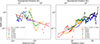 |
Fig. 6. Jet collimation profile of the receding counter-jet (left) and approaching jet (right) derived from stacked images at all frequencies using pixel-by-pixel analysis. The jet width is plotted as a function of distance from the common reference frame. Power-law fits (solid red lines) indicate a parabolic expansion for both sides, with indices k = 0.47 ± 0.01 (counter-jet) and k = 0.66 ± 0.01 (jet), consistent with magnetically collimated flows. |
By fitting a power-law model to describe the jet width d as a function of distance r, we found the best-fit power-law indices of k = 0.66 ± 0.01 for the jet and k = 0.47 ± 0.01 for the counter-jet, indicating a nearly parabolic shape on both sides. This result is further supported by an additional analysis we performed using all MODELFIT components from both epochs (see Appendix A Fig. A.3), which yielded best-fit power-law indices of k = 0.554 ± 0.01 for the jet and k = 0.604 ± 0.01 for the counter-jet. For this analysis, we excluded components with FWHM values smaller than half of the beam minor axis to avoid unresolved features that could bias the fit. The consistency between these findings and the pixel-by-pixel analysis of the stacked image reinforces the conclusion of a parabolic jet shape.
To investigate any potential changes in jet geometry, we tested for a transition in the jet shape by fitting a broken power law. The half opening angle profile (Fig. 7) does indicate the existence of a transition, showing an initial steep decrease and then a flattening with a roughly constant half opening angle beyond 5 mas from the core (corresponding to a de-projected distance of 1.05 × 10⁵ RS, expressed in Schwarzschild radii). In this region, the half–opening angle is estimated to be approximately 4.5° (with a full opening angle of 9°). In our analysis, the apparent half opening angle θhalf(r) is derived from the measured jet width W(r) via the relation θhalf(r) = arctan[0.5 W(r)/r], where r is the projected distance from the core. The observed flattening of the profile beyond 5 mas suggests a possible transition from parabolic to conical geometry in the jet. Parabolic or semi-parabolic shapes are commonly observed in the innermost jet regions (within a few parsecs), with a transition to conical geometry occurring when the collimation ends (Kovalev et al. 2020; Boccardi et al. 2021).
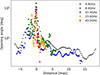 |
Fig. 7. Opening angle profiles of the counter-jet and jet as a function of projected distance from the common reference frame derived from pixel-by-pixel Gaussian width fits applied to the stacked VLBI images at all frequencies. |
We modeled the collimation profile using a broken power-law function of the form
![Mathematical equation: $$ \begin{aligned} d(r) = d_{\rm t} \cdot 2^{(u-w)/h} \cdot \left(\frac{r}{r_{\rm t}}\right)^{u} \cdot \left[1 + \left(\frac{r}{r_{\rm t}}\right)^{h}\right]^{(w-u)/h}, \end{aligned} $$](/articles/aa/full_html/2026/05/aa57764-25/aa57764-25-eq8.gif) (4)
(4)
where u and w are the power-law indices before and after the transition, dt is the jet width at the transition point, rt marks the transition distance, and h controls the sharpness of the break. However, the fit did not yield a statistically significant improvement over the single power-law description: The break location was poorly constrained, and the residuals near the transition region remained large. Further analysis with a richer dataset providing better sampling of the outer jet regions is required for a more robust test, as additional epochs of high-sensitivity multifrequency observations would increase the signal-to-noise ratio and better recover the faint extended emission in the outer jet and allow for more precise measurements of the jet width on VLBI scales. In addition, complementary lower-frequency and lower-resolution observations would help sample larger spatial scales and provide a more solid description of the jet’s conical region. These complementary data would support a more robust broken power-law fit with tighter constraints on the break point and the power-law indices. Nevertheless, the opening angle profile suggests that a transition is occurring around 105 RS. Interestingly, we observed a significant enhancement in the flux density both in the jet side and in the counter-jet side at this distance (Fig. 3). This enhancement is best seen visually in the 5 GHz images (e.g., top-left panel in Fig. 2) at 3.5 mas and 7 mas in the jet and counter-jet sides, respectively (see also Table A.1). When applying the proper shifts, these features were found to be equidistant from the BH location and to coincide with the proposed occurrence of the jet shape transition at 5 mas, or 105 RS. Such bright recollimation features, which are typically stationary, have been observed in other sources at the end of the acceleration and collimation zone (e.g., Boccardi et al. 2016; Hada et al. 2018), marking the region where the jet stops being magnetically driven or, alternatively, signaling a change in the external pressure profile (see also Asada & Nakamura 2012). In this context, a comparison with the acceleration estimates derived from the jet-to-counter-jet ratio (Sect. 3.2) suggests that the bulk of the acceleration occurs within ≲3 × 10⁴ RS, that is, on smaller scales with respect to the putative collimation break near ∼105 RS.
3.5. Spectral index distribution
To investigate the spectral properties along the jet, we employed a pixel-based analysis analogous to that used for our stacked-image analysis (Sect. 2.3). All natural weighted maps were first aligned in the common reference frame as described in Sect. 2.2. For each frequency pair, we convolved both maps to a common circular beam with a diameter equal to the average of the two beams and used a pixel size equal to one-fifth of this average beam. We divided the jet and counter-jet into one-pixel-wide slices across the jet ridge line. We then extracted the flux density in each slice across the jet ridge line by integrating the fit Gaussian profile. Slices were retained only in regions where the signal in both images exceeded five times the value of the RMS to ensure reliable measurements.
The spectral index (α) was calculated for each slice as
where Sν is the flux density at frequency ν, S0 is the reference flux at frequency ν0, and α is the spectral index. We included uncertainties by propagating thermal noise (pixel RMS) and calibration errors assumed to be 5% for the 4.9−8.4 GHz pairs and 10% for the higher-frequency pairs.
Figure 8 shows α as a function of the projected distance from the common reference frame for four frequency pairs. The core region (within ∼2 mas) exhibits an inverted spectrum (α > 2), indicative of optically thick synchrotron self-absorbed emission. At the highest frequencies (> 15 GHz), the spectral index exceeds the value of +2.5, which is the theoretical limit for a purely synchrotron self-absorbed emission region. This could indicate that free-free absorption is also taking place, but only in a very compact region at the jet base, which becomes resolved at the highest frequencies. This aspect will be investigated in more detail in a follow-up paper. Further downstream, α becomes steep, reflecting optically thin emission. In the innermost counter-jet and jet regions, the spectral index reaches very steep values (α ∼ −2.5) at higher frequencies, increasing to more typical optically thin values (α ∼ −1) at larger distances. Similar steep spectral index behavior has been reported in other sources, such as NGC 315 and M 87 (Ricci et al. 2025; Ro et al. 2023). In particular, Ricci et al. (2025) suggest that such steep values may result from particles being accelerated via diffusive shock acceleration in strongly magnetized plasma and subsequently undergoing significant synchrotron cooling losses. The recurrence of this behavior across different sources indicates that steep spectral indices may be a common feature of jets in their parabolic collimation region.
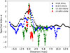 |
Fig. 8. Spectral index profile (α) along the jet ridge line of 3C 452 measured from four frequency pairs 4.9/8.4 GHz (black triangles), 8.4/15.4 GHz (blue squares), 15.4/23.6 GHz (green diamonds), and 23.6/43.2 GHz (red circles). The horizontal axis shows the projected distance in milliarcseconds from the common reference frame, and the vertical axis shows the spectral index computed via Sν ∝ να. The central region (within ∼2 mas) displays strongly inverted spectra (α > 2), which are indicative of synchrotron self-absorption, while downstream values turn negative, consistent with optically thin synchrotron emission. The peak in the spectral index near 0 mas supports the adopted reference position of the black hole. |
4. Comparison with Cygnus A and other HEGs
The twin-jet systems in 3C 452 and Cygnus A offer a unique opportunity to investigate jet collimation and acceleration processes in narrow-line FRII radio galaxies on sub-parsec scales. While Cygnus A has long served as a benchmark for studies of collimated jet formation in powerful sources, the new multifrequency VLBI observations of 3C 452 provide a valuable opportunity to test similar physical processes in a different environment. Both sources exhibit two-sided jets observed at large viewing angles and are still sufficiently bright on sub-parsec scales at millimeter wavelengths.
The jet expansion profiles in the two objects indicate a parabolic jet shape well described by power-law fits. In 3C 452, the jet and counter-jet follow r ∝ z0.66 and r ∝ z0.47, respectively, with the parabolic geometry persisting to approximately 105 RS. In Cygnus A, the jet shows a similar parabolic profile with r ∝ z0.55 up to ∼104 RS, beyond which it briefly becomes cylindrical before transitioning to a conical profile (Boccardi et al. 2016). Therefore, while the jet expansion rates are similar, the extent of the parabolic region is larger in 3C 452 than in Cygnus A by an order of magnitude. Additionally, 3C 452 has an Eddington ratio of L/LEdd ≈ 0.03 (log(L/LEdd)≈ − 1.46, with MBH = ∼8 × 10⁸ M⊙) based on the uniform hard X-ray selected AGN measurements in the Swift BAT AGN Spectroscopic Survey (BASS) Data Release 2 (DR2) catalog (Koss et al. 2022). Similarly, Cygnus A has L/LEdd ≈ 0.02 (log(L/LEdd)≈ − 1.74, with MBH = ∼2.7 × 10⁹ M⊙) from the same catalog. Although Cygnus A hosts a more massive black hole, the similarity in their low Eddington ratios suggests that the order-of-magnitude difference in the extent of their parabolic jet regions is not driven by gross differences in accretion rate but instead reflects intrinsic differences in jet collimation and interaction with the surrounding medium.
It has been proposed that jet collimation transitions may occur near the Bondi radius in some AGNs, which is the radius at which the black hole’s gravity dominates the thermal motion of the hot gas. In some sources, such as M 87 and NGC 6251, the parabolic–to–conical jet transition occurs near the Bondi radius, suggesting a possible connection between the external pressure profile and jet collimation (e.g., Asada & Nakamura 2012; Tseng et al. 2016). In other objects (e.g., NGC 315, NGC 4261), the transition occurs well inside the Bondi scale (e.g., Boccardi et al. 2021; Balmaverde et al. 2008; Kovalev et al. 2020). The powerful FR II Cygnus A maintains a parabolic profile out to ∼104 RS (Boccardi et al. 2016), well inside the estimated Bondi radius of ∼3 × 10⁵ RS (Nakahara et al. 2019). Detailed analysis of the jet width profile in Cygnus A has also shown a discontinuity in the jet width profile at distances on the order of 2.3 × 10⁵ − 6.8 × 10⁵ RS, where the downstream jet appears to widen relative to the upstream trend, roughly at distances near the Bondi radius (Nakahara et al. 2019). For 3C 452, we cannot make a similar comparison since existing X-ray observations do not provide measurements of the hot gas temperature on scales close to the black hole that are required to estimate the Bondi radius, precluding a meaningful estimate for this source.
It is also instructive to compare the terminal jet opening angles among these two powerful radio galaxies. Boccardi et al. (2016) reported an intrinsic full opening angle of approximately ∼10° for Cygnus A. In 3C 452, the apparent full opening angle flattens near ∼9° (Fig. 7), which, considering a viewing angle of ∼70°, corresponds to an intrinsic full opening angle of ∼8.4°, in close agreement with the case of Cygnus A. Such opening angles are large compared to the intrinsic values typically derived for blazars (∼1°, e.g., Pushkarev et al. 2017), and they are indicative of mildly relativistic Lorentz factors (Γ ∼ 1 − 2). Assuming a transversely stratified jet, the Lorentz factor Γ ∼ 9 derived in Sect. 3.3 possibly reflects the bulk speed of the de-boosted filaments of the flow, while the geometrical properties of the radio emission are dominated by a slower component that is the brightest at large viewing angles. At such angles, relativistic Doppler de-boosting suppresses emission from the fast spine, making the slower sheath more prominent and leading to a lower apparent speed. In this case, the high Lorentz factor is obtained by assuming that the low observed brightness temperatures are mainly due to Doppler de-boosting. However, if the low brightness temperatures instead arise from intrinsic jet properties, such as intrinsic high magnetization in an accelerating and magnetically dominated flow, strong Doppler de-boosting would not be required. In that case, similar viewing angles could be obtained with Doppler factors closer to unity, implying lower intrinsic jet speeds and Lorentz factors, consistent with previous studies. Therefore, the derived Lorentz factor depends on the assumed origin of the observed brightness temperatures and does not uniquely determine the intrinsic bulk flow speed.
A notable distinction is that Cygnus A clearly exhibits limb-brightened emission and transversely stratified velocity fields, which are suggestive of a spine-sheath configuration with a fast central spine surrounded by a slower layer. Limb-brightening is not observed in 3C 452. This may indicate that such a transverse structure is intrinsically not present or, alternatively, that it remains unresolved. Owing to the higher redshift of 3C 452, the transverse spatial resolution achieved by our 43 GHz VLBI observations corresponds to physical scales on the order of ≳103 RS, thus significantly larger than the ∼400 RS scales resolved in Cygnus A at the same observing frequency (Boccardi et al. 2016). Therefore, achieving comparable transverse spatial resolution in 3C 452 would require higher-frequency VLBI observations at 86 GHz, which would probe spatial scales on the order of ≲103 RS.
It is also interesting to compare the findings for 3C 452 and Cygnus A with those obtained in the literature for other HEGs. Indeed, jet collimation studies have considered several other objects belonging to this class but characterized by a smaller viewing angle of the jet. Analysis of the jet expansion profiles in powerful broad-line AGN have revealed very extended collimation zones, with transitions typically observed beyond 106 RS (e.g., Boccardi et al. 2021). In fact, Cygnus A was the only HEG in the sample of Boccardi et al. (2021) with a transition distance consistent with the shorter scales commonly seen in LEGs. Our new results place 3C 452 firmly alongside Cygnus A, making it a second example of a FRII HEG with a comparatively compact collimation region.
Figure 9 presents the distribution of the transition distances for 15 HEGs reported in the literature (Boccardi et al. 2021; Algaba et al. 2019; Traianou et al. 2020; Okino et al. 2022; Burd et al. 2022; Yi et al. 2024; Shang et al. 2025) together with 3C 452. We divided the sample into two groups: narrow-line HEGs viewed at large angles (Cygnus A and 3C 452) and broad-line HEGs (including several flat-spectrum radio quasars (FSRQs), such as CTA 26, PKS 0528+134, 4C +71.07, 4C +29.45, and 3C 279) viewed at smaller angles. All broad-line HEGs exhibit jet shape transitions at 106 − 107 RS. In contrast, Cygnus A and 3C 452 lie one to two orders of magnitude below this range. Since we expect all of these sources to have intrinsically similar properties, this comparison might indicate that the determination of the jet transition distance has a dependence on the jet orientation. For instance, if the jet does have a spine-sheath transverse structure, it is possible that these two components collimate on different scales.
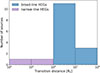 |
Fig. 9. Distribution of the de-projected transition distances in HEGs, expressed in units of Schwarzschild radii (RS). Data were compiled from Boccardi et al. (2021), Algaba et al. (2019), Traianou et al. (2020), Okino et al. (2022), Burd et al. (2022), Yi et al. (2024), Shang et al. (2025) and also include 3C 452. Narrow-line HEGs (Cygnus A and 3C 452) are plotted in purple, while broad-line HEGs are shown in blue. |
In sources seen close to the line of sight, such as FSRQs, the spine dominates and appears to collimate out to very large distances, whereas in narrow-line radio galaxies, such as 3C 452 and Cygnus A, the sheath may define the observed break scale. The number statistics for narrow-line HEGs are clearly still very limited, which highlights the importance of studies considering fainter sources such as 3C 452 for understanding jet formation in powerful sources.
5. Conclusions
We have presented a detailed multifrequency VLBI study of the twin-jet system in the FRII radio galaxy 3C 452 based on high-resolution observations at 5−43 GHz. The availability of both the jet and counter-jet across all frequencies enabled us to probe the jet structure symmetrically on sub-parsec scales, offering rare insights into the collimation and physical conditions at the jet base of an FRII system viewed at a large inclination. Moreover, we note that the double-double morphology of this source, with faint large-scale relic lobes beyond the classical FRII lobes (Sirothia et al. 2013), suggests restarted activity, while the misalignment between sub-parsec and kiloparsec jet position angles (Fig. 1) may indicate variations in nuclear properties over time. Our main results can be summarized as follows:
-
We find that the jet-to-counter-jet intensity ratio (Rj/cj) remains nearly constant at lower frequencies, implying that the emission is dominated by intrinsic jet properties and is less affected by nuclear variability or opacity effects. In contrast, at higher frequencies and within the inner ∼1−1.5 mas, Rj/cj increases sharply, consistent with an increasing jet speed near the jet base. Beyond ∼2 mas, the ratio levels off, indicating that the jet speed is approximately constant on larger scales.
-
Combined constraints from Rj/cj and brightness temperatures yield a viewing angle of θ ≈ 70° and an intrinsic speed of β ≈ 0.99c, consistent with the source’s classification as a lobe-dominated FRII galaxy. The low Doppler factors (δ ∼ 0.03 − 0.83) further support minimal beaming effects. Our orientation constraints are in good agreement with previous estimates, including the lower limit of θ ≥ 60° from Giovannini et al. (2001) and the upper limit of θmax = 78.7° ±1.0° from Boccardi et al. (2025).
-
Our analysis revealed a remarkable symmetry between the two jets in the collimation properties. The jet and counter-jet follow a near-parabolic expansion, with power-law indices of k = 0.66 ± 0.01 and k = 0.47 ± 0.01, respectively. The opening angle profile flattens at ∼105 RS, indicating a possible transition in the jet shape. At the same distance, bright symmetric features are observed on both sides, consistent with stationary recollimation structures that may mark the end of the collimation region. A comparison of the profile of Rj/cj with distance indicates that most of the acceleration occurs upstream of this distance.
-
Our pixel-based spectral index analysis revealed a strongly inverted core spectrum (α > +2 within ∼2 mas). At the highest frequencies, the core spectrum exceeds the synchrotron self-absorption limit (+2.5), pointing to the presence of additional absorption processes in a very compact region at the jet base. Further out, the spectrum steepens to optically thin values, with very steep indices (α ∼ −2.5) in the inner jet regions, a behavior also observed in other nearby radio galaxies such as NGC 315 and M 87.
-
The distribution of the transition distances in a sample of HEGs shows that broad-line sources exhibit jet-shape transitions at 106 − 107 RS, whereas the narrow-line objects 3C 452 and Cygnus A fall one to two orders of magnitude below this range. This suggests that orientation plays an important role in the observed collimation scale.
Taken together, these results show that 3C 452 emerges as a rare and valuable analog to Cygnus A, allowing us to probe jet collimation and symmetry in a second narrow-line FRII galaxy. This outcome also highlights the importance of orientation in shaping the observed properties of powerful jets in HEGs.
Data availability
The VLBI images associated with this article are available at the CDS via https://cdsarc.cds.unistra.fr/viz-bin/cat/J/A+A/709/A89
Acknowledgments
The authors thank the anonymous referee for their valuable feedback. E.M., B.B., and L.R. acknowledge financial support from an Otto Hahn Research Group funded by the Max Planck Society. E.M. is a member of the International Max Planck Research School (IMPRS) for Astronomy and Astrophysics at the Universities of Bonn and Cologne. This work is based on observations obtained with the Very Long Baseline Array (VLBA) and the Effelsberg 100-m radio telescope. The VLBA is a facility of the National Science Foundation operated under cooperative agreement by Associated Universities, Inc. The European VLBI Network is a joint facility of European, Chinese, South African, and other radio astronomy institutes funded by their national research councils.
References
- Algaba, J. C., Rani, B., Lee, S. S., et al. 2019, ApJ, 886, 85 [NASA ADS] [CrossRef] [Google Scholar]
- Asada, K., & Nakamura, M. 2012, ApJ, 745, L28 [NASA ADS] [CrossRef] [Google Scholar]
- Balmaverde, B., Baldi, R. D., & Capetti, A. 2008, A&A, 486, 119 [NASA ADS] [CrossRef] [EDP Sciences] [Google Scholar]
- Black, A. R. S., Baum, S. A., Leahy, J. P., et al. 1992, MNRAS, 256, 186 [NASA ADS] [Google Scholar]
- Blandford, R. D., & Königl, A. 1979, ApJ, 232, 34 [Google Scholar]
- Blandford, R., Meier, D., & Readhead, A. 2019, ARA&A, 57, 467 [NASA ADS] [CrossRef] [Google Scholar]
- Boccardi, B., Krichbaum, T. P., Bach, U., et al. 2016, A&A, 585, A33 [NASA ADS] [CrossRef] [EDP Sciences] [Google Scholar]
- Boccardi, B., Krichbaum, T. P., Ros, E., & Zensus, J. A. 2017, A&ARv, 25, 4 [NASA ADS] [CrossRef] [Google Scholar]
- Boccardi, B., Perucho, M., Casadio, C., et al. 2021, A&A, 647, A67 [NASA ADS] [CrossRef] [EDP Sciences] [Google Scholar]
- Boccardi, B., Ricci, L., Madika, E., et al. 2025, A&A, 695, A118 [NASA ADS] [CrossRef] [EDP Sciences] [Google Scholar]
- Burd, P. R., Kadler, M., Mannheim, K., et al. 2022, A&A, 660, A1 [NASA ADS] [CrossRef] [EDP Sciences] [Google Scholar]
- Buttiglione, S., Capetti, A., Celotti, A., et al. 2010, A&A, 509, A6 [NASA ADS] [CrossRef] [EDP Sciences] [Google Scholar]
- Fanaroff, B. L., & Riley, J. M. 1974, MNRAS, 167, 31P [Google Scholar]
- Fioretti, V., Angelini, L., Mushotzky, R. F., Koss, M., & Malaguti, G. 2013, A&A, 555, A44 [NASA ADS] [CrossRef] [EDP Sciences] [Google Scholar]
- Giovannini, G., Cotton, W. D., Feretti, L., Lara, L., & Venturi, T. 2001, ApJ, 552, 508 [NASA ADS] [CrossRef] [Google Scholar]
- Greisen, E. W. 1990, in Acquisition, Processing and Archiving of Astronomical Images, eds. G. Longo, & G. Sedmak, 125 [Google Scholar]
- Hada, K., Doi, A., Wajima, K., et al. 2018, ApJ, 860, 141 [NASA ADS] [CrossRef] [Google Scholar]
- Heckman, T. M., & Best, P. N. 2014, ARA&A, 52, 589 [Google Scholar]
- Homan, D. C., Cohen, M. H., Hovatta, T., et al. 2021, ApJ, 923, 67 [NASA ADS] [CrossRef] [Google Scholar]
- Kadler, M., Ros, E., Lobanov, A. P., Falcke, H., & Zensus, J. A. 2004, A&A, 426, 481 [NASA ADS] [CrossRef] [EDP Sciences] [Google Scholar]
- Kharb, P., Lister, M. L., & Cooper, N. J. 2010, ApJ, 710, 764 [NASA ADS] [CrossRef] [Google Scholar]
- Koss, M. J., Ricci, C., Trakhtenbrot, B., et al. 2022, ApJS, 261, 2 [NASA ADS] [CrossRef] [Google Scholar]
- Kovalev, Y. Y., Pushkarev, A. B., Nokhrina, E. E., et al. 2020, MNRAS, 495, 3576 [NASA ADS] [CrossRef] [Google Scholar]
- Krause, M. G. H., Shabala, S. S., Hardcastle, M. J., et al. 2019, MNRAS, 482, 240 [CrossRef] [Google Scholar]
- Leahy, J. P., Bridle, A. H., & Strom, R. G. 1996, An Atlas of DRAGNs (3CRR Atlas), http://www.jb.man.ac.uk/atlas/, online archive of radio images for 3CRR sources, accessed via NASA NED [Google Scholar]
- Lee, S.-S., Lobanov, A. P., Krichbaum, T. P., et al. 2008, AJ, 136, 159 [Google Scholar]
- Lobanov, A. P. 1998, A&A, 330, 79 [NASA ADS] [Google Scholar]
- Nakahara, S., Doi, A., Murata, Y., et al. 2019, ApJ, 878, 61 [NASA ADS] [CrossRef] [Google Scholar]
- Okino, H., Akiyama, K., Asada, K., et al. 2022, ApJ, 940, 65 [NASA ADS] [CrossRef] [Google Scholar]
- Paraschos, G. F., Kim, J. Y., Krichbaum, T. P., & Zensus, J. A. 2021, A&A, 650, L18 [NASA ADS] [CrossRef] [EDP Sciences] [Google Scholar]
- Pushkarev, A. B., Kovalev, Y. Y., Lister, M. L., & Savolainen, T. 2017, MNRAS, 468, 4992 [Google Scholar]
- Readhead, A. C. S. 1994, ApJ, 426, 51 [Google Scholar]
- Ricci, L., Boccardi, B., Nokhrina, E., et al. 2022, A&A, 664, A166 [NASA ADS] [CrossRef] [EDP Sciences] [Google Scholar]
- Ricci, L., Boccardi, B., Röder, J., et al. 2025, A&A, 693, A172 [NASA ADS] [CrossRef] [EDP Sciences] [Google Scholar]
- Ro, H., Kino, M., Sohn, B. W., et al. 2023, A&A, 673, A159 [NASA ADS] [CrossRef] [EDP Sciences] [Google Scholar]
- Shang, H., Zhao, W., Hong, X., & Hu, X.-Z. 2025, ApJ, 986, 198 [Google Scholar]
- Shelton, D. L., Hardcastle, M. J., & Croston, J. H. 2011, MNRAS, 418, 811 [Google Scholar]
- Shepherd, M. C. 1997, ASP Conf. Ser., 125, 77 [Google Scholar]
- Sirothia, S. K., Gopal-Krishna, & Wiita, P. J. 2013, ApJ, 765, L11 [Google Scholar]
- Traianou, E., Krichbaum, T. P., Boccardi, B., et al. 2020, A&A, 634, A112 [NASA ADS] [CrossRef] [EDP Sciences] [Google Scholar]
- Tseng, C.-Y., Asada, K., Nakamura, M., et al. 2016, ApJ, 833, 288 [NASA ADS] [CrossRef] [Google Scholar]
- Véron-Cetty, M. P., & Véron, P. 2006, A&A, 455, 773 [Google Scholar]
- Yi, K., Park, J., Nakamura, M., Hada, K., & Trippe, S. 2024, A&A, 688, A94 [NASA ADS] [CrossRef] [EDP Sciences] [Google Scholar]
The excitation index is defined as EI = log[O III]/Hβ − 1/3(log[N II]/Hα+log[S II]/Hα+log[O I]/Hα) (Buttiglione et al. 2010).
Appendix A: Images and MODELFIT parameters
 |
Fig. A.1. VLBI images of 3C 452 from project BM516A. From top to bottom: 4.9 GHz, 8.4 GHz, 15.4 GHz, and 23.6 GHz. Left panels: images with uniform weighting. Right panels: images with natural weighting. |
 |
Fig. A.2. VLBI images of 3C 452 from project BM516B. From top to bottom: 4.9 GHz, 8.4 GHz, 15.4 GHz, 23.6 GHz, and 43.2 GHz. Left panels: images with uniform weighting. Right panels: images with natural weighting. |
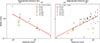 |
Fig. A.3. Collimation profile of the receding counter-jet (left) and approaching jet (right) derived from MODELFIT components at all frequencies and epochs. Only fully resolved components located at distances larger than one beam from the core and with FWHM larger than half the beam minor axis are included. The fit power-law indices are consistent with those obtained from the pixel-based analysis (see Fig. 6), confirming the parabolic expansion of both jets. The shaded Fit Error band is included in the legend but is very small compared to the data scatter and thus not easily visible in the plot. |
Properties of the MODELFIT Gaussian components for the multifrequency VLBI observations of 3C 452, from project code BM516A.
Properties of the MODELFIT Gaussian components for the multifrequency VLBI observations of 3C 452, from project code BM516B.
MODELFIT core component and map parameters used to derive the core resolution limit and brightness temperature at all frequencies for BM516A and BM516B.
All Tables
Log of observations and characteristics of the clean maps forming the multifrequency dataset.
Properties of the MODELFIT Gaussian components for the multifrequency VLBI observations of 3C 452, from project code BM516A.
Properties of the MODELFIT Gaussian components for the multifrequency VLBI observations of 3C 452, from project code BM516B.
MODELFIT core component and map parameters used to derive the core resolution limit and brightness temperature at all frequencies for BM516A and BM516B.
All Figures
|
Fig. 1. Twin-jet structure of 3C 452 from kiloparsec to sub-parsec scales. The top image was obtained from VLA data at 1.4 GHz (Leahy et al. 1996). The following maps show the VLBI structure at different frequencies (4.9 GHz, 8.4 GHz, 15.4 GHz, 23.6 GHz, 43.2 GHz) based on the analyzed data of our project code BM516B presented in Sect. 2. Images were produced using natural weighting. The maps have been aligned to the central brightest feature. The complete series of images considered in the article is presented in the Appendix A. |
| In the text | |
|
Fig. 2. Stacked VLBI images of 3C 452 at 4.9 (upper left), 8.4 (upper right), 15.4 (middle left), 23.6 (middle right), and 43.2 (bottom) GHz. The images were restored with circular beams of 1.48, 0.8, 0.45, 0.34, and 0.18 mas, respectively. The respective peak flux density and rms values are displayed at the top of each panel. The maps were produced using uniform weighting. |
| In the text | |
|
Fig. 3. Flux density profiles of the receding counter-jet (left panel) and approaching jet (right panel) and as a function of distance from the common reference frame, measured from the stacked images at each frequency. The profiles were derived using pixel-based Gaussian fitting across transverse jet slices, as described in Sect. 2.3. |
| In the text | |
|
Fig. 4. Jet-to-counter-jet intensity ratio as a function of frequency. Ratios are derived for three datasets: BB393, BM516A, and BM516B. All images were aligned to the common reference frame, identified as the midpoint between the jet and counter-jet cores in the 43 GHz map (Sect. 2.2). The BB393 observations were published in Boccardi et al. (2025). |
| In the text | |
|
Fig. 5. Jet-to-counter-jet intensity ratio as a function of distance from the common reference frame, shown for all observing frequencies. The analysis includes data from projects BB393, BM516A, and BM516B. |
| In the text | |
|
Fig. 6. Jet collimation profile of the receding counter-jet (left) and approaching jet (right) derived from stacked images at all frequencies using pixel-by-pixel analysis. The jet width is plotted as a function of distance from the common reference frame. Power-law fits (solid red lines) indicate a parabolic expansion for both sides, with indices k = 0.47 ± 0.01 (counter-jet) and k = 0.66 ± 0.01 (jet), consistent with magnetically collimated flows. |
| In the text | |
|
Fig. 7. Opening angle profiles of the counter-jet and jet as a function of projected distance from the common reference frame derived from pixel-by-pixel Gaussian width fits applied to the stacked VLBI images at all frequencies. |
| In the text | |
|
Fig. 8. Spectral index profile (α) along the jet ridge line of 3C 452 measured from four frequency pairs 4.9/8.4 GHz (black triangles), 8.4/15.4 GHz (blue squares), 15.4/23.6 GHz (green diamonds), and 23.6/43.2 GHz (red circles). The horizontal axis shows the projected distance in milliarcseconds from the common reference frame, and the vertical axis shows the spectral index computed via Sν ∝ να. The central region (within ∼2 mas) displays strongly inverted spectra (α > 2), which are indicative of synchrotron self-absorption, while downstream values turn negative, consistent with optically thin synchrotron emission. The peak in the spectral index near 0 mas supports the adopted reference position of the black hole. |
| In the text | |
|
Fig. 9. Distribution of the de-projected transition distances in HEGs, expressed in units of Schwarzschild radii (RS). Data were compiled from Boccardi et al. (2021), Algaba et al. (2019), Traianou et al. (2020), Okino et al. (2022), Burd et al. (2022), Yi et al. (2024), Shang et al. (2025) and also include 3C 452. Narrow-line HEGs (Cygnus A and 3C 452) are plotted in purple, while broad-line HEGs are shown in blue. |
| In the text | |
|
Fig. A.1. VLBI images of 3C 452 from project BM516A. From top to bottom: 4.9 GHz, 8.4 GHz, 15.4 GHz, and 23.6 GHz. Left panels: images with uniform weighting. Right panels: images with natural weighting. |
| In the text | |
|
Fig. A.2. VLBI images of 3C 452 from project BM516B. From top to bottom: 4.9 GHz, 8.4 GHz, 15.4 GHz, 23.6 GHz, and 43.2 GHz. Left panels: images with uniform weighting. Right panels: images with natural weighting. |
| In the text | |
|
Fig. A.3. Collimation profile of the receding counter-jet (left) and approaching jet (right) derived from MODELFIT components at all frequencies and epochs. Only fully resolved components located at distances larger than one beam from the core and with FWHM larger than half the beam minor axis are included. The fit power-law indices are consistent with those obtained from the pixel-based analysis (see Fig. 6), confirming the parabolic expansion of both jets. The shaded Fit Error band is included in the legend but is very small compared to the data scatter and thus not easily visible in the plot. |
| In the text | |
Current usage metrics show cumulative count of Article Views (full-text article views including HTML views, PDF and ePub downloads, according to the available data) and Abstracts Views on Vision4Press platform.
Data correspond to usage on the plateform after 2015. The current usage metrics is available 48-96 hours after online publication and is updated daily on week days.
Initial download of the metrics may take a while.