| Issue |
A&A
Volume 709, May 2026
|
|
|---|---|---|
| Article Number | A242 | |
| Number of page(s) | 20 | |
| Section | Extragalactic astronomy | |
| DOI | https://doi.org/10.1051/0004-6361/202558663 | |
| Published online | 25 May 2026 | |
Higher-resolution optical spectra of M*< 1010 M⊙ galaxies reveal outflow signatures unresolved by the SDSS
1
Institute of Theoretical Astrophysics, University of Oslo, P.O. Box 1029 Blindern 0315, Oslo, Norway
2
Dipartimento di Fisica e Astronomia Augusto Righi, Università degli Studi di Bologna, Via Gobetti 93/2, 40129 Bologna, Italy
3
INAF – Osservatorio di Astrofisica e Scienza dello Spazio di Bologna, Via Gobetti 101, 40129 Bologna, Italy
4
INAF – Osservatorio Astronomico di Brera, Via Brera 28, 20121 Milano, Italy
5
INAF – Fundación Galileo Galilei, Rambla José Ana Fernandez Pérez 7, 38712 Breña Baja, TF, Spain
6
Armagh Observatory and Planetarium, College Hill, Armagh BT61 9DG, UK
7
Max-Planck-Institut für Radioastronomie, Auf dem Hügel 69, 53121 Bonn, Germany
8
Department of Physics and Astronomy, University College London, London WC1E 6BT, UK
9
INAF – Osservatorio Astronomico di Padova, Vicolo dell’Osservatorio 5, 35122 Padova, Italy
★ Corresponding author: This email address is being protected from spambots. You need JavaScript enabled to view it.
Received:
18
December
2025
Accepted:
1
April
2026
Abstract
Galactic outflows are predicted to be ubiquitous in low-mass galaxies, but observational evidence is lacking. Both a low signal-to-noise ratio and a low spectral resolution can severely hamper the detection of galactic outflows, especially in small galaxies that have intrinsically narrow spectral lines. In an effort to overcome these issues, we obtained new, medium-high resolution (FWHMinst ∼ 50 − 110 km/s) optical spectra of 52 local star-forming galaxies (0.01 < z < 0.03) with stellar masses 108.5 < M*/[M⊙]< 1010, using the TNG/DOLORES and NTT/EFOSC2 instruments. Our parent sample consists of galaxies from the Sloan Digital Sky Survey (SDSS) with available heterodyne single-dish molecular (i.e., CO) line data. The targets of this study are selected among those that, based on the comparison between CO line widths, SDSS spectral resolution, and corresponding SDSS-based Hα line widths, have a high chance of being unresolved by SDSS spectroscopy. Our new, medium-high resolution spectra reveal overall narrower Hα and [OIII]λ5007 lines, with signs of asymmetries and broad wings that are absent in the SDSS spectra of the same galaxies. This confirms our hypothesis that SDSS spectroscopy does not resolve the narrow emission lines of low-M* galaxies, which hinders the detection of outflows. We identify outflow signatures in ∼30% of our targets based on the Hα line spectra. Assuming a typical bi-conical outflow geometry, this detection rate is consistent with theoretical predictions of ubiquitous outflows in the low-mass regime. The outflow incidence is enhanced (∼60%) for galaxies with above average star-formation rates (SFR) for the sample (SFR > 10−0.74 M⊙/yr). We estimate ionized gas mass outflow rates ranging from ∼0.1 − 50 × 10−3 M⊙/yr (mean ∼20 × 10−3 M⊙/yr) and corresponding mass loading factors between 0.03 and 0.14 (mean ∼0.07) for the sample.
Key words: galaxies: evolution / galaxies: general / galaxies: ISM / galaxies: kinematics and dynamics
© The Authors 2026
 Open Access article, published by EDP Sciences, under the terms of the Creative Commons Attribution License (https://creativecommons.org/licenses/by/4.0), which permits unrestricted use, distribution, and reproduction in any medium, provided the original work is properly cited.
This article is published in open access under the Subscribe to Open model. This email address is being protected from spambots. You need JavaScript enabled to view it. to support open access publication.
1. Introduction
In the Λ cold dark matter (ΛCDM) cosmological model, galaxies grow within a network of dark matter filaments, through a finely tuned exchange of material between their interstellar medium (ISM), the surrounding circum-galactic medium (CGM), and the external environment. Galactic outflows are thought to be key actors in this “baryon cycle” as they can transport gas and dust away from galaxy nuclei and disks, possibly carrying some beyond the virial radius, hence depleting the ISM and regulating star formation. This is likely instrumental in “quenching”, i.e., the transition of galaxies from star-forming to quiescent (Veilleux et al. 2005, 2020). The exact physical mechanisms behind quenching remains one of the central unsolved questions in the theory of galaxy evolution.
Outflows are generally multiphase (e.g., Cicone et al. 2018), requiring multiwavelength observations to fully characterize. Observations of a single phase, such as those of the warm ionized phase we present here, cannot be used to fully constrain mass outflow rates, for instance, particularly since the colder, denser phases frequently dominate the outflow mass (e.g., Carniani et al. 2015; Fluetsch et al. 2021; Hagedorn et al. 2026). Nonetheless, they are useful for determining the incidence of outflows and informing follow-up observations at complementary wavelengths.
Theoretical models predict that quenching due to outflows driven by star formation is most effective in low-mass galaxies, since gas is more easily ejected from their shallow gravitational potentials (Dekel & Silk 1986; Mac Low & Ferrara 1999; Ferrara & Tolstoy 2000; Veilleux et al. 2005; Davé et al. 2011). This has been suggested as an explanation for the decreasing stellar mass to halo mass relation in the low-mass regime (Behroozi et al. 2010). In addition, outflows are predicted to effectively remove metals from the ISM of low-mass galaxies (Christensen et al. 2018), offering one possible explanation for the low observed fractions of metals retained in these objects (McQuinn et al. 2015) and the resulting mass-metallicity relation (Brooks et al. 2007). Outflows have also been invoked as an explanation for the “core” dark matter halos of dwarf galaxies (Navarro et al. 1996; Governato et al. 2010, 2012; Teyssier et al. 2013).
All this suggests that outflows should be near-ubiquitous in the low-mass regime. Such outflows have, indeed, been observed in ionized gas tracers (e.g., Manzano-King et al. 2019; McQuinn et al. 2019; Xu et al. 2022; Marasco et al. 2023). However, some studies covering wide ranges of stellar mass report that outflow incidence declines with stellar mass (e.g., Cicone et al. 2016; Concas et al. 2017; Avery et al. 2021). This may be due to the fact that detecting outflow signatures requires high-quality data, and spectroscopic galaxy surveys at optical wavelengths are generally not optimized for outflow identification. Commonly used techniques for identifying outflows rely on analysis of the kinematics of the gas through observations of spectral lines in emission or absorption (e.g., Rupke & Veilleux 2011; Cicone et al. 2014). Outflows produce signatures in the profiles of spectral lines in the form of faint, possibly asymmetric, high-velocity features, distinct from those produced by ISM components in gravitationally dominated motion. Detecting faint features naturally requires high signal-to-noise (S/N) spectra, while deviations from line profiles produced by rotating disks can only be seen in spectra with sufficient spectral resolution to resolve such details of the line profile. The former issue can be overcome to some extent by spectral stacking (e.g., Cicone et al. 2016; Concas et al. 2017), but the latter requires the use of appropriate instruments, especially in the case of low-mass galaxies, which have overall narrower line profiles, which may not be resolved in optical spectra from galaxy surveys such as the Sloan Digital Sky Survey (SDSS). It is therefore somewhat unclear whether the low incidence of outflows in the low-mass regime is in contrast to theoretical predictions or whether it is due to the lack of quality data in this regime.
In this work, we present medium-high resolution optical spectroscopy of 52 local galaxies (0.01 < z < 0.03) with stellar masses (M*) between 108.5 M⊙ and 1010 M⊙, and with emission lines unresolved by SDSS spectroscopy (hereafter we refer to the new data simply as high-resolution). This sample is selected from galaxies observed in carbon monoxide (CO(1−0) or CO(2−1)) emission with single-dish heterodyne instruments on the APEX and IRAM telescopes as part of the ALLSMOG and xCOLDGASS surveys. The very high spectral resolution of the molecular line observations allows us to identify candidates that are potentially unresolved in optical SDSS spectra (see Section 2 for details on the selection process).
The paper is structured as follows. In Section 2, we outline the sample selection. In Section 3, we describe the observations and data reduction process. Section 4 describes the methods used in fitting the emission line profile and identifying the outflows. In Section 5, we show the effect of the improved spectral resolution and and derive the outflow incidence for the sample. In Section 6, we discuss the implications of our results with respect to previous observations and theoretical predictions. In Section 7, we offer a brief summary and conclude with the main findings of this work. Throughout this paper, we assume a flat ΛCDM cosmology with parameters from the Planck Collaboration VI (2020) (H0 = 67.7 km s−1 Mpc−1, Ωm = 0.31, ΩΛ = 0.69) for cosmological distance calculations.
2. Target selection
Our targets are drawn from a parent sample sample of galaxies with available molecular line coverage, specifically from the single-dish ALLSMOG (Bothwell et al. 2014; Cicone et al. 2017; Hagedorn et al. 2024) and xCOLDGASS (Saintonge et al. 2017) surveys, and photometry and spectroscopy from SDSS DR8 (Aihara et al. 2011). We explain our sample selection below, which relies on a comparison between CO and Hα line widths.
Figure 1 shows the Hα emission line widths obtained from the SDSS spectra (using a single-Gaussian fit accounting for instrumental resolution, see Section 4.1) as a function of the CO line widths adopted from ALLSMOG and xCOLDGASS for all CO detections in the respective samples. For galaxies with line widths larger than the SDSS spectral resolution (i.e., to the right of the vertical dashed red line in Fig. 1) there is a correlation between Hα and CO line widths. We also note that in this regime, CO appears systematically broader than Hα. This is likely due to the 3″ SDSS fiber probing only the center of these galaxies, while the CO observations cover a much larger part of the disk (see further discussion in Section 5.1). To the left of the vertical dashed red line (i.e., below the SDSS spectral resolution), the Hα line widths inferred from SDSS spectroscopy scatter around a value of ∼100 km/s regardless of the associated CO line widths, and the correlation between Hα and CO line widths breaks down. This is further illustrated by the deviation between the binned median line width (black line) and the extrapolation to lower FWHM values of the linear fit performed on the spectrally resolved (higher-FWHM) data (dashed blue line in Fig. 1). This is clearly a resolution effect, and it strongly indicates that some of the M* ≲ 1010 M⊙ galaxies are unresolved by SDSS spectroscopy, and so their Hα line width measurements are dominated by instrumental dispersion and associated uncertainties. We confirm this in Appendix A, where we compare the line widths obtained from SDSS spectra directly to those obtained from higher-resolution spectra.
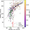 |
Fig. 1. Full width at half maximum (FWHM) of the Hα line from SDSS DR8 vs. FWHM of CO from ALLSMOG and xCOLDGASS. The dotted red line shows the velocity resolution equivalent of R = 2000 (FWHM ∼ 150 km/s), which is typical for SDSS DR8 at this redshift. The dashed gray line shows the one-to-one relation. Galaxies targeted with high-resolution spectroscopy are marked with green diamonds. Targets without detections in CO are marked with vertical line markers on the x-axis at the position corresponding to their SDSS-inferred Hα line widths. The dashed black and white line shows the running median in logarithmic bins of 0.2 dex width. The solid blue line shows a linear fit to the data with resolved Hα lines (i.e., to the right of the R = 2000 line), which is extrapolated into the unresolved regime as a dashed line. The color scaling corresponds to the stellar mass of the galaxies. |
The goal of this study is to test whether the low SDSS resolution could hide ionized outflow signatures in low M* galaxies. The targets of our TNG/DOLORES and NTT/EFOSC2 follow-up that are detected in CO are marked in Fig. 1 using green diamonds. To avoid biases towards especially gas-rich galaxies, our sample also includes galaxies without CO detections that span the same range of SDSS-based inferred Hα line widths. The targets were selected to have M* < 1010 M⊙, z < 0.05 and SDSS-based Hα line widths below the SDSS resolution. For observations with TNG/DOLORES, we further restricted the targets to magR < 17.5 and magV < 17. For observations with NTT/EFOSC2 magnitudes were restricted to magR < 18.5 and magV < 18.5. Magnitudes were calculated on the basis of the magnitudes in the r- and g-bands measured in the SDSS fiber. We adopted stellar masses from the MPA-JHU value-added catalog1 for SDSS DR8 and redshifts from ALLSMOG and xCOLDGASS. Based on these criteria, targets were selected to efficiently fill the allocated observing nights and minimize air mass during observations. Due to weather-induced changes in the schedule for the NTT/EFOSC2 observations, we observed some additional targets not in the originally selected sample, some of which had magnitudes in the R- and V-band between 18.5 and 19 (2MASSJ00114318+1428010, LEDA1397680, and UGC11992). The full target list of 52 galaxies is reported in Table B.1 in Appendix B.
Our sample ranges in stellar mass from ∼108.5 M⊙ and ∼1010 M⊙ and in star-formation rates (SFR) from ∼10−2.5 M⊙/yr and ∼1 M⊙/yr. The majority of galaxies in the sample are star-forming based on the criterion defined in Hagedorn et al. (2024) using the offset from the main sequence of star-forming galaxies as defined by Saintonge & Catinella (2022). Four targets (SDSSJ011437.36+011053.4, SDSSJ120108.03+152353.6, UGC11992, and LEDA213877) lie far enough below the main sequence to be defined as quiescent using this definition. Using emission line diagnostics (Baldwin et al. 1981; Kewley et al. 2001; Kauffmann et al. 2003), one galaxy in the sample (SDSSJ120108.03+152353.6) shows active galactic nucleus (AGN)-like ionization, and one (NGC2607) is classified as low-ionization nuclear emission-line region (LINER)-like. The remaining galaxies show star-formation-like ionization, except for LEDA213877, which could not be classified due to its lack of detected emission lines in both SDSS and TNG spectra.
3. Data
We obtained high-resolution spectroscopy of 52 local galaxies. The targets are listed in Table B.1 and the emission line spectra used in this work are shown in Appendices C and D.
3.1. TNG/DOLORES observations
Of our sample, 14 targets were observed with TNG/DOLORES between 3 March and 5 March 2024 (Program ID: A48TAC_16, PI: C. Vignali). We obtained long-slit spectroscopy using the V510 and V656 grisms covering wavelength ranges of 4875 − 5325 Å and 6232 − 6888 Å respectively. For the redshift range of our sample, this coverage includes, respectively, the [OIII]λ5007 (hereafter simply [OIII]) and Hα emission lines. With a 1.0″ slit and a 1 × 1 binning, this resulted in a nominal spectral resolution of R ∼ 5950 for the V510 setup and R ∼ 5248 for the V656 setup. With each grism, we took a single exposure of between 800 s and 3200 s for each target, based on its SDSS fiber magnitudes in the r- and g-bands. The slit was positioned on the peak of the galaxy’s brightness profile in the acquisition image, and its orientation was chosen to minimize atmospheric effects during the long exposures, and its alignment relative to the galaxy’s geometry is therefore essentially random. Examples of spectra with clearly detected emission lines are shown in Fig. 2. Weather conditions were mixed, with seeing varying between 0.5″ and 2.0″.
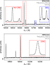 |
Fig. 2. Example spectra obtained with TNG/DOLORES spectroscopy using the V656 and V510 grisms with a 1.0″ slit. We note that these spectra do not have their absolute flux calibrated, so units on the y-axis are arbitrary. The dashed gray line shows the zero flux level. Insets show a more detailed view of select emission lines, with the size of the zoomed-in region shown by the dashed colored boxes. |
3.2. NTT/EFOSC2 observations
The remaining 38 galaxies were observed with NTT/EFOSC2 (Program IDs: 113.269W, PI: B. Hagedorn). For 25 we have coverage of both [OIII] using grism#19 (gr19, covering 4441−5114 Å) and Hα using grism#20 (gr20, 6047−7147 Å), while eight were observed only in [OIII] and five only in Hα. With both grisms, a 0.5″ slit and a 1 × 1 binning were used, leading to nominal spectral resolutions of R ∼ 3338 for gr19 and R ∼ 3281 for gr20. Again, the slit was centered on the brightest part of the galaxy and its alignment was not matched to the galaxy’s geometry. With each grism, we took a single exposure of between 800 s and 2810 s for each target, based on its SDSS fiber magnitudes in the r- and g-bands. For the additional fainter targets mentioned in Section 2, we took two exposures of 2810 s each. Examples of spectra with clearly detected emission lines are shown in Fig. 3. Weather conditions were mixed, with seeing varying between 1.0″ and 2.0″.
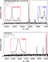 |
Fig. 3. Example spectra obtained with NTT/EFOSC2 spectroscopy using grisms 20 and 19 with a 0.5″ slit. We note that these spectra do not have their absolute flux calibrated, so units on the y-axis are arbitrary. The dashed gray line shows the zero flux level. Insets show a more detailed view of select emission lines, with the size of the zoomed-in region shown by the dashed colored boxes. |
3.3. CO(1–0) and CO(2–1) data
From the ALLSMOG and xCOLDGASS surveys, we obtained spectra of the CO(1−0) and CO(2−1) emission lines where available. We used the FWHM reported in Cicone et al. (2017) and Saintonge et al. (2017) in our analysis. The native spectral resolution of the heterodyne instruments used for these observations is extremely high (R ∼ 105 − 106, although most spectra are rebinned to increase S/N), hence CO line width measurements are not limited by spectral resolution.
Of 52 galaxies in our sample, 35 are detected in CO emission at the 3σ level and 17 are non-detections. The CO emission line spectra used in this work are shown alongside the optical emission line spectra in Appendices C and D.
3.4. Data reduction
We used version 1.17.4 of PypeIt2 (Prochaska et al. 2020b,a), a Python package for semi-automated reduction of astronomical slit-based spectroscopy, to reduce both TNG/DOLORES and NTT/EFOSC2 spectroscopy. PypeIt has specific default parameter configurations for both EFOSC2 and DOLORES, which we adopted for the reduction process.
Since our analysis focuses on emission lines rather than continuum emission, we used a boxcar extraction profile with a radius of 1.5″ for the extraction of 1D spectra to ensure we did not exclude emission line flux in cases where its spatial distribution deviates from that of the continuum. For observations with EFOSC2’s gr19, no strong sky lines fall into the observed wavelength range, so we did not perform a correction for flexure in the spectral direction.
For wavelength calibration and to determine the spectral resolution, we used the 1D spectra of the arc lamp calibration exposures taken at the beginning of each night. We find a median spectral resolution (FWHM) of 78 km/s (52 km/s) for Hα with EFOSC2/gr20 (DOLORES/V656) and 114 km/s (48 km/s) for [OIII] with EFOSC2/gr19 (DOLORES/V510). The spectral resolution for [OIII] with EFOSC2/gr19 is comparatively poor because the line is close to the limit of the spectral range.
4. Analysis
4.1. Emission line fitting
For a first assessment of the S/N (which we define as the amplitude of the emission line divided by the rms of the spectrum estimated from line-free regions) of the targeted emission lines and to estimate their width, we performed an initial fit to the spectra in regions around the Hα (6535−6600 Å) and [OIII] (4985−5025 Å) emission lines. We subtracted a constant pseudo-continuum3 from the 1D spectra extracted from NTT/EFOSC2 and TNG/DOLORES spectroscopy around the Hα and [OIII] emission lines and used the standard deviation of the flux density in the line-free parts of the spectra to estimate the noise level.
We used the lmfit python package (Newville et al. 2014) to fit both the Hα and [OIII] lines with a single Gaussian function, in a range corresponding to a Doppler shift of ±350 km/s from the expected line center based on the redshift retrieved from the SDSS data. In the case of the Hα line, the [NII] doublet is also modeled with a set of two Gaussian functions with shared kinematics (central velocity and velocity dispersion) and with relative amplitudes fixed at a ratio of 0.34. The Gaussian emission line templates are convolved with the instrumental resolution of EFOSC2 or DOLORES, as applicable, before fitting. Based on this initial fit, we consider an emission line detected if it has S/N > 3. Of 43 galaxies observed in Hα, 39 are detected, and for [OIII] we detected 26 out of 46 observed galaxies. The line widths obtained from the initial fit are listed in Table B.2 of Appendix B.
4.2. Fitting of line wings
To account for the presence of potential outflow signatures in the high-resolution spectroscopy, we iteratively fitted the Hα and [OIII] emission lines with a more flexible model once the line center and overall dispersion were determined. This model uses up to three independent Gaussian components that are fitted simultaneously to the continuum-subtracted line spectrum. This enables us to model both blue- and redshifted wings, which may not be symmetric in the presence of dust extinction from the disk or from the outflow itself (see, e.g., Hagedorn et al. 2026). For each Gaussian component velocity dispersion σ, is constrained to be greater than the instrumental resolution at the wavelength of observation. Other parameters are left free to vary within the spectral range of the fit (±350 km/s). This range was chosen after a visual inspection of the spectra to be broad enough to include any high-velocity features but narrow enough to exclude neighboring lines, such as the [NII] doublet around Hα. We fitted in a three-step iterative process (with one, two, and three Gaussian components, respectively) using the PySpecKit package (Ginsburg et al. 2022; Ginsburg & Mirocha 2011) with initial parameters informed by the residuals of the fit in the previous iteration. Due to the high resolution of the spectra and the narrow emission lines in the target galaxies, there is no blending between the Hα line and the nearby [NII] doublet (see examples in Figures 2 and 3), which allowed us to fit the Hα line in isolation in this step.
The best-fit model is chosen from among the three iterations based on the Akaike information criterion (AIC, Akaike 1974). Each Gaussian component contributes three free parameters to the model, and the maximum likelihood is estimated from the residual sum of squares of the range of the fit, which we used to determine the number of independent data points.
We do not immediately assume that a best-fit model with more than one component implies the presence of outflows, since these components may trace other mechanisms, such as tidal structures, unresolved merging companions, or inflows. Instead, we use the distribution of central velocities and velocity dispersions to identify likely outflow signatures as described in Section 5.4.
5. Results
5.1. Comparison between high-resolution Hα and CO line widths
We used Hα line widths inferred from the initial single-Gaussian fit to the new high-resolution spectra to test the effects of an improved Hα spectral resolution on the relation between Hα and the CO line widths previously shown in Fig. 1. The results are shown in Fig. 4, which includes the original SDSS data points for comparison (gray dots). The Hα FWHM values measured with the higher-resolution data are, as expected, smaller than the SDSS values measured previously. As a result, the correlation between CO and Hα line widths holds down to the lowest FWHM values. The downturn that was visible in Fig. 1 has disappeared, confirming that it was due to the insufficient SDSS resolution that made an accurate determination of Hα line widths impossible in this regime.
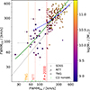 |
Fig. 4. Same as Fig. 1, but with line widths inferred from high-resolution spectroscopy replacing data unresolved by SDSS (the unresolved data are still shown as gray dots). The solid green line shows a linear fit to the combined SDSS resolved and high-resolution data. The solid blue line shows the same linear fit to the resolved SDSS data as in Fig. 1, extrapolated to the SDSS-unresolved regime as a dashed line. Targets without detections in CO are marked with vertical line markers on the x-axis at the position corresponding to their Hα line widths inferred from their NTT or TNG spectra. Dotted vertical lines show the approximate SDSS resolution R = 2000 (FWHM ∼ 150 km/s), and the median resolution for the sample achieved with TNG (FWHM ∼ 52 km/s) and NTT (FWHM ∼ 78 km/s) for the Hα line. |
Moreover, thanks to the new higher-resolution data, we can confirm the trend of broader CO than Hα lines even in the low M* regime. Differences in aperture size and placement between optical observations and SDSS (3″ fiber), TNG (1″), NTT (0.5″), and the CO observations with APEX (27″ at 1.3 mm) and IRAM (22″ at 3 mm) are likely a major factor in this systematic difference. In Appendix A, where we compare Hα line widths inferred from SDSS with the new values computed from the higher-resolution spectra, we show that such aperture effects are unlikely to play a significant role in the observed differences in optical line widths between SDSS on the one hand and TNG and NTT on the other, however.
5.2. Hα line wings and asymmetries
For galaxies in which the Hα emission line is detected at sufficiently high S/N, we searched for the presence of high-velocity wings or asymmetries. Such features can indicate galaxy-scale outflows that may have remained undetected in the unresolved SDSS spectra.
We compute the excess kurtosis (hereafter simply kurtosis) of the Hα line profile in the sample to assess the presence of high-velocity wings. The kurtosis of a distribution, or fourth standardized moment, measures its “tailed-ness”, so for emission lines with broad wings due to outflows we expect an excess kurtosis relative to a Gaussian line profile. Measures of kurtosis of the emission line profile have previously been used to identify galactic outflows in integrated spectroscopy (Yu et al. 2022). To ensure that the kurtosis measurement is not dominated by noise, we calculate the kurtosis using the spectral range where the emission line exceeds three times the rms noise level of the spectrum. We calculate the kurtosis in this way for galaxies that are detected at S/N > 10 in Hα, to exclude galaxies for which this cut would remove significant amounts of flux, possibly distorting the line profile. This leaves us with a subsample of 33 galaxies.
Fig. 5 shows the Hα line profile kurtosis for each galaxy calculated from SDSS spectroscopy versus that calculated from the high-resolution NTT or TNG data. The SDSS spectroscopy produces line profiles with kurtosis values between ±0.5, whereas the values for the high-resolution spectra are scattered more broadly, with a few notable examples exhibiting kurtosis values > 1. This is because the lines are unresolved in the SDSS spectroscopy, resulting in line shapes close to the approximately Gaussian instrumental profile and the corresponding expected kurtosis of zero. Galaxies with above average SFR (median SFR = 10−1 M⊙/yr for galaxies in the sample with kurtosis measurements) tend to also exhibit leptokurtic line profiles (i.e., kurtosis > 0), as expected if the excess kurtosis is due to wing emission from high-velocity gas in star-formation-driven outflows.
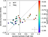 |
Fig. 5. Comparison between line profile kurtosis of SDSS spectra and corresponding high-resolution observations. The color scale corresponds to the SFR of each galaxy measured in the SDSS fiber. The error bars in the bottom right show the typical statistical uncertainty on the calculated values. |
We perform a similar test using non-parametric percentile velocities v02, v50, and v98, which correspond to the range Doppler velocities in which 2.3%, 50%, and 97.7% of the total emission line flux are contained. We used the difference between the absolute values of v02 and v98 to assess asymmetries in the spectra. Blueshifted asymmetries (i.e., |v02|−|v98|> 0) are usually interpreted as signatures of outflows (e.g., Cicone et al. 2016), where emission from redshifted outflowing gas is attenuated by dust in the galaxy disk. We adjusted both velocities by the central velocity of the line v50, to account for possible differences in line centroids, which may be due to either aperture (i.e., SDSS fiber vs. slit of the NTT/TNG spectra) or to slit positioning effects, especially for targets that are very extended. On average, we find a difference of ∼15 km/s in v50 between SDSS and higher-resolution spectra. An extreme example of this is the spectrum of UGC7017, for which there is a significant velocity shift in the lines observed with SDSS spectroscopy versus those in the high-resolution spectra (see Fig. D.2). UGC7017 is much more extended than the 3″ SDSS fiber, making it susceptible to aperture and targeting effects.
After this adjustment, the difference |v02 − v50|−|v98 − v50| should primarily capture asymmetries in the line profile, with positive values corresponding to excess flux on the blueshifted side of the profile, and negative values to excess flux on the redshifted side. From Fig. 6 it is evident that the high-resolution data cover a wider range of values in this parameter, with a few notable examples exceeding 20 km/s. Most galaxies exhibiting strong blueshifted asymmetries in Hα also have leptokurtic line profiles (see magenta circles in Fig. 6). We thus confirm the presence, in several targets, of line asymmetries compatible with galactic outflows, which remain undetected in the lower-resolution SDSS spectra.
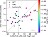 |
Fig. 6. Comparison between absolute percentile velocity differences. The color scale corresponds to the SFR of each galaxy measured in the SDSS fiber. Magenta circles mark galaxies with leptokurtic Hα line profiles (i.e., kurtosis > 0). The error bars in the bottom right show the typical statistical uncertainty on the calculated values. |
5.3. Comparison of [OIII]5007 and Hα line profiles
In the previous sections, we focused on the Hα emission line as a tracer of ionized gas kinematics, since we have more and higher S/N detections of this line in our sample than of the [OIII] line. In the following, we will compare the Hα and [OIII] lines in galaxies in our high-resolution sample where they are both detected, before moving on to the identification and characterization of outflows in the data.
The observed [OIII] lines are generally broader than the Hα lines in these galaxies, as can be seen in the top panel of Fig. 7. However, this trend appears to be driven mainly by observations with NTT/EFOSC2. In these, the [OIII] line falls close to the end of the wavelength range covered by the grism used (gr19), which results in a relatively poor spectral resolution (∼100 km/s). After subtracting the instrumental dispersion in quadrature for both lines (bottom panel in Fig. 7), the data are scattered around the one-to-one relation between the two lines. We caution that line widths derived from single-component Gaussian fits may not accurately characterize a well-resolved line profile, especially if there are asymmetries or broad wings present. In Section 5.4, we compare the two lines in greater detail with a fit function that is better suited to model any additional components detected in the line profiles.
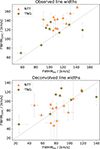 |
Fig. 7. Comparison between Hα and [OIII]5007 line widths observed with high-resolution spectroscopy (top) and deconvolved from instrumental resolution (bottom). |
5.4. Outflow characterization
To account for the asymmetries and non-Gaussianity of line profiles observed in the new high-resolution spectra, we perform a fit with the multi-component model described in Section 4.2. The plots with the best-fit models are shown in Appendices C and D and the results are shown in Tables B.2 and 1. The best-fit model requires a single Gaussian component for 24, two components for 12, and three components for three of 39 galaxies with Hα detections. For the 26 [OIII] detected galaxies, these numbers are 23, two, and one, respectively. Using the same fitting routine for the SDSS data shows that all line profiles are best described with a single Gaussian.
Outflow properties.
Fig. 8 shows the central velocity v and dispersion σ of the components from the best-fit models across all 15 (3) galaxies in which the Hα ([OIII]) line is detected and required more than one component to fit. We divide between narrow components (σ < 60 km/s) with small velocity offsets (|v|< 30 km/s) and broad or blueshifted components, which exceed either of the criteria. We classify the former as tracing quiescent ISM, while the latter trace potential outflow signatures. The limits for this classification scheme are chosen so that line components that account for a majority of the total flux of the emission line (Fcomp/Ftot > 0.5) all lie within the bounds we adopt for quiescent components, as shown by the color scale in Fig. 8, and components that lie outside of the chosen boundaries are all broad or blueshifted but not redshifted, which is consistent with the expected signatures of outflowing high-velocity gas. In cases where both blueshifted and redshifted outflowing high-velocity gas is observed, this leads to relatively symmetric broad wings in the emission line profile, corresponding to the components in the upper half of the plots in Fig. 8. Where the redshifted side of the outflow is attenuated by extinction from dust in the galaxy disk and only the blueshifted part of the outflow is observed, the line profiles show a blue asymmetry, corresponding to components on the left in Fig. 8.
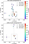 |
Fig. 8. Central velocity v and velocity dispersion σ of all components in the best-fit multi-Gaussian model across all galaxies in which the relevant line is detected and required multiple components to fit. The top panel shows the results of the fit to the Hα emission line and the bottom panel the [OIII] emission line. The color scale shows the flux of the component relative to the total flux summed over all components in the best-fit model. The dashed gray rectangle corresponds to ±30 km/s in v and 60 km/s in σ, and marks the separation between components tracing potential outflow signatures and those tracing rotating gas. Numbering of the components only reflects the order in which they are added during the iterative fitting procedure. |
In the absence of additional constraints on the kinematics of the quiescent ISM (e.g., from stellar kinematics), the accuracy of this classification scheme is uncertain. However, we find good agreement of the scheme with the non-parametric measures described in Section 5.2. Components outside the adopted bounds are all associated with lines that have relatively high kurtosis (> 0.35) or blue excess (|v02 − v50|−|v98 − v50|> 20 km/s).
Of 39 galaxies with a detection of Hα in our sample, ten show potential outflow signatures (26%), when applying the above criteria. For [OIII] this is true for only three out of 26 (12%). However, if we consider only galaxies with emission line detections at S/N > 10, we observe potential outflow signatures in 10 of 33 (30%) of galaxies in Hα and 3 of 12 (26%) in [OIII].
Two effects may play a role in this. On the one hand, typically faint outflow-like components are more likely to go undetected in low S/N spectra, and on the other hand, stronger emission lines correlate with higher SFR, which is linked to outflow incidence.
Galaxies with a high S/N > 10 detection of at least one of the Hα and [OIII] lines, and in which an outflow is detected in at least one of these two tracers, have a median star-formation rate of log(SFR/[M⊙ yr−1]) = − 0.72 and a median stellar mass of log(M*/[M⊙]) = 9.38 compared to log(SFR/[M⊙ yr−1]) = − 1.41 and log(M*/[M⊙]) = 9.31 for galaxies with S/N > 10 in at least one tracer but no outflow detection in either. So, even when correcting for S/N effects, the incidence of outflows is higher for higher SFRs, as is to be expected if feedback from star formation is the primary driver for these outflows.
6. Discussion
In this section, we estimate the physical properties of the observed outflows and use them to infer the mass outflow rates and the mass loading factors. We also discuss the results of our outflow analysis in the context of previous observations and theoretical predictions of the incidence of outflow in the low-M* regime. Before we do so, it is important to point out the limitations of integrated spectroscopy for the purpose of outflow identification. Although the broad and asymmetric components we identify in the observed emission line profiles are consistent with signatures expected from outflowing gas, they could, in principle, also be attributed to inflowing gas, merging companions, components of tidal origin, or even rotation. Without knowledge of where the emitting gas is located relative to the galaxy and the observer, it is not possible to conclusively break this degeneracy.
However, it is reassuring that the potential outflow signatures we identify are all blueshifted relative to their quiescent counterparts (see Fig. 8). This is consistent with extinction from the ISM affecting signatures of redshifted outflow components, which must be on the far side of the galaxy disk from the observer. For inflows, the effect of extinction, if present, would be reversed, and we would expect to see more redshifted high-velocity components if there were a significant contribution from inflowing gas in our sample. Nonetheless, it is possible that our analysis overestimates the real outflow incidence rate by including galaxies in which inflows, mergers, or similar events produce kinematic signatures indistinguishable from outflows using integrated spectroscopy.
We also note that our sample is not representative of the low-mass galaxy population in general, due to selection and sensitivity effects. The outflow incidence we find in the sample, therefore, is not a measure of the incidence in the overall population of low-mass galaxies.
6.1. Observed outflow incidence in the local universe
Previous studies of the local galaxy population generally report that outflows are common in star-forming main-sequence galaxies with M* ≳ 1010 M⊙ (e.g., Chen et al. 2010; Cicone et al. 2016; Avery et al. 2021). Chen et al. (2010) use nebular sodium doublet (NaI D) absorption to identify outflows and find incidence fractions of around 30% at the high-mass end of their sample. Similarly, Roberts-Borsani & Saintonge (2019), report a prevalence of neutral atomic outflows in star-forming galaxies with M* ≳ 1010 M⊙ based on their stacking analysis of nebular sodium absorption in SDSS DR7 galaxies. Based on MaNGA integral field spectroscopy, Avery et al. (2021) identify outflows in 12% of their sample, the vast majority in galaxies with M* ≳ 1010 M⊙, where the incidence fraction is > 20%. Both of these studies report a sharp drop in the outflow incidence below M* ∼ 1010 M⊙, with incidence fractions of only a few percent in the lower masses. Similarly, Concas et al. (2017) find no evidence of outflows in galaxies with M* < 1010 M⊙ in their analysis of the [OIII] line in stacked SDSS spectra.
Our results show that the outflow incidence in our sample of low-mass galaxies is strikingly similar to that at higher masses, when measured based on high-resolution spectroscopy, indicating that the drop-off observed in previous studies based on optical emission lines may be largely due to insufficient spectral resolution to resolve outflows in the lower-mass regime. Indeed, quite strikingly, we have demonstrated that SDSS spectroscopy already at M* ∼ 1010 M⊙ does not fully resolve optical emission line profiles, indicating that any outflow studies (or line profile studies) in this mass regime are hampered by resolution effects. For studies using sodium absorption to trace the neutral atomic phase, the difference in outflow incidence at low and high masses could be due to other effects, such as the absence of dust that makes NaI D ineffective as a tracer (Roberts-Borsani & Saintonge 2019).
Outflows in low-mass galaxies have been successfully detected with high-resolution spectroscopy in small samples of local galaxies (Manzano-King et al. 2019; Xu et al. 2022; Marasco et al. 2023). The low-velocity nature of the outflows described in Xu et al. (2022) and Marasco et al. (2023) also supports the explanation that their kinematic signatures would not be detectable with lower resolution spectroscopy, leading to the trend with stellar mass observed in other studies (Chen et al. 2010; Concas et al. 2017; Avery et al. 2021). Manzano-King et al. (2019) find outflow signatures in 13 of 50 (26%) galaxies in their mixed sample of objects with and without indicators of AGN ionization and masses between 108 M⊙ and 1010 M⊙ observed with Keck/LRIS with a spectral resolution of σ ∼ 80 km/s. This is similar to the incidence we find here, although most of the outflow candidates in their sample are associated with AGN activity, whereas none of the outflow candidates in our sample show clear signs of AGN activity.
6.2. Comparison to theoretical predictions for low-mass galaxies
In this section we discuss the outflow incidence in our sample in light of the ubiquity of galactic winds invoked to explain a number of phenomena such as the observed stellar mass to halo mass relation (Behroozi et al. 2010), low metal fraction of dwarf galaxies (McQuinn et al. 2015), and properties of their dark matter halos (Navarro et al. 1996; Governato et al. 2010, 2012; Teyssier et al. 2013). An incidence fraction of ∼30% may seem low in light of these predictions, but it is important to keep in mind the limitations of observational techniques for the identification of outflows. Spectroscopic identification of outflows depends on the presence of gas with line-of-sight velocities distinct from those of quiescent gas in the ISM.
If a typical outflow has a bi-conical morphology with an opening angle of θ = 45°, which is consistent with detailed observations in the local universe (Venturi et al. 2018; López-Cobá et al. 2020), it subtends a solid angle of Ωout = 4π(1 − cos θ)≈3.7. The probability of observing outflowing gas in the line of sight can then be approximated as Ωout/(4π)≈0.3. An observed outflow incidence fraction of ∼30% would, with these assumptions, be consistent with near-ubiquitous outflows in the sample. This interpretation is in line with the argument made by Carniani et al. (2024), who applied the same considerations to a sample of low-mass galaxies at higher redshift and reported an outflow incidence of 25%–40%.
The timescales of star formation and outflow lifetimes may also have an effect on the observed incidence. Even if all galaxies are affected by outflows over the course of their evolution, these events could be relatively short-lived in galaxies where star formation happens in short bursts.
6.3. Mass loading
In this section, we estimate the mass loading factor η = Ṁout/SFR of the outflows observed in our sample. As we do not have information on the extent of the outflows, we need to assume one. The results should therefore be treated as order-of-magnitude estimates.
Since our higher-resolution spectra are not calibrated in terms of absolute flux, we combine them with integrated line fluxes derived from SDSS spectra to estimate outflow masses. To this end, we multiply the fraction of the flux contained in the outflow component(s) (see Section 5.4 and Table B.2) by the integrated line flux of the Hα line measured in the SDSS fiber. We adopt Hα fluxes from Hagedorn et al. (2024), where they are derived from a full-spectrum fit to the SDSS spectra using the GandALF code (Sarzi et al. 2006), which takes into account Hα absorption in the stellar continuum and dust extinction. After converting the resulting integrated outflow fluxes to luminosities, we obtain outflow masses following Fluetsch et al. (2021).
As an estimate for the outflow velocity, we use |v02| (see Section 5.2). Finally, we estimate the physical extent of the outflow to be comparable to the size of the galaxy, adopting r50, the radius containing 50% of the Petrosian r-band flux, obtained from SDSS DR8 (Aihara et al. 2011), as the outflow extent. We then calculate the outflow mass rates as
This results in a median outflow mass rate of Ṁout = 10−2 Ṁ/yr and a mean mass loading factor of ∼0.07. Table 1 lists the outflow properties for the individual galaxies in the sample.
This is about an order of magnitude lower than what is reported in McQuinn et al. (2019), but consistent with observations by Marasco et al. (2023), both of which use Hα to trace the warm ionized outflows. The latter point out that these discrepancies are within what is expected from differences in methods used to measure outflows.
Comparing the mass loading factors derived here with theoretical predictions is not trivial. Our observations measure only the warm ionized phase of the gas, whereas cosmological simulations generally do not distinguish different gas phases and are therefore likely to report higher-mass outflow rates than observations of a single tracer. Based on the EAGLE simulations, Mitchell et al. (2020) predict mass loading factors of ∼1 − 3 in the mass range of our sample, exceeding our results by at least an order of magnitude. Similarly, Nelson et al. (2019) predict η ∼ 3 − 10, based on the TNG50 simulations, about two orders of magnitude higher than what we find here. This implies either that the warm ionized phase of the outflow accounts for only about 1% of the mass outflow rate in these galaxies, that theoretical feedback recipes lead to more extreme outflows than observed, or a combination thereof.
Observations of outflows in ultra-luminous infrared galaxies (ULIRGs) using multiple tracers show mass rate contributions < 1% in these objects (Fluetsch et al. 2021). The well-studied outflow in the local starburst M82 shows a similar partition, with the warm ionized phase contributing only a small fraction of the mass outflow rate (Shopbell & Bland-Hawthorn 1998) compared to the neutral atomic (Contursi et al. 2013) and cold molecular (Leroy et al. 2015) phases, consistent with the contribution of ∼1% our results imply. Romano et al. (2023) report mass loading factors of the order of unity in the neutral atomic phase of outflows in a sample of low-mass galaxies, which would be consistent with a small contribution from the ionized phase in combination with our estimates. Due to the generally low S/N of the available CO observations, we were unable to investigate the presence of cold gas counterparts to the ionized outflows in our sample directly.
We tested the dependence of the outflow properties in the sample on the SFR, M*, and the molecular gas fraction fmol = Mmol/M* by splitting the sample into two bins for each of these quantities. To demarcate the bins, we used the median of the outflowing sample in each case (SFR, M*, and fmol). We adopted the molecular gas fractions for the eight galaxies with CO detections from Hagedorn et al. (2024). The results are listed in Table 1. The outflow velocities are consistent across the bins, given the associated statistical uncertainties. Uncertainties on the derived outflow properties, mass rate, and mass loading, are generally high, so that no significant differences can be determined between bins. The most pronounced difference is in the mass outflow rate of galaxies with fmol > 0.16 versus those with fmol < 0.16, the former showing a higher-mass outflow rate, if only at ∼1σ significance.
Table 1 also shows outflow incidence fractions (compared to all galaxies with Hα S/N > 10 falling into the relevant bin) for the different bins described above. Incidence is enhanced in the high SFR, whereas differences are negligible in the M* and fmol bins, given the size of the sample. The behavior with SFR is not surprising for a regime in which we expect primarily star-formation-driven outflows. Following the arguments made in Section 6.2, the enhanced incidence for high-SFR galaxies may also imply larger average outflow opening angles in this regime.
7. Summary and conclusion
We present high-resolution TNG and NTT spectroscopy for 52 local galaxies with stellar masses below 1010 M⊙. Comparing gas velocity dispersions inferred from the Hα and [OIII] line profiles in the high-resolution data to those inferred from SDSS data shows that SDSS spectroscopy does not resolve emission line profiles in these objects. As a result, asymmetries and broad wings evident in the high-resolution spectra, quantified by excess kurtosis and non-parametric velocity measures, are largely absent in the low-resolution SDSS spectroscopy, where line profiles are dominated by the instrumental dispersion profile.
We investigate whether these features correspond to potential galactic outflows and find that ∼30% of galaxies in our sample with Hα or [OIII] emission lines detected at S/N > 10 show signatures of potential outflows, which account for between 10% and 40% of the total integrated line flux. The lack of outflow detections at stellar masses below 1010 M⊙ in local galaxies reported in some studies based on optical emission lines (e.g. Cicone et al. 2016; Concas et al. 2017; Avery et al. 2021) is therefore likely due to the use of low-spectral resolution data, in which the narrow emission lines of low-mass galaxies are not sufficiently resolved to identify outflow signatures. Based on the fraction of line flux attributed to the outflows, we estimate the median mass loading factor in the outflow sample to be ∼0.07. This is consistent with predictions from numerical simulations (Nelson et al. 2019; Mitchell et al. 2020) if the warm ionized phase of the outflow contributes about 1% of the total mass loading, which is supported by multi-phase observations (Fluetsch et al. 2021; Heckman & Thompson 2017).
Assuming that outflows in the low-mass regime present predominantly as bi-conical structures with opening angles of 45°, the incidence of outflows of ∼30% we find in our sample suggests that outflows are near-ubiquitous in the low-mass regime. This is consistent with predictions from theoretical works, which invoke such outflows to regulate star formation (Dekel & Silk 1986; Mac Low & Ferrara 1999; Ferrara & Tolstoy 2000; Behroozi et al. 2010; Davé et al. 2011), eject metals from the ISM (McQuinn et al. 2015; Brooks et al. 2007), and shape the dark matter halos (Navarro et al. 1996; Governato et al. 2010, 2012; Teyssier et al. 2013) in low-mass galaxies. We observe enhanced incidence fractions for galaxies with above-average SFR and Hα S/N in the sample, as expected for star-formation-driven outflows.
Acknowledgments
We thank the anonymous referee for their insightful comments. This work makes use of data from the Sloan Digital Sky Survey (SDSS). Funding for SDSS-III has been provided by the Alfred P. Sloan Foundation, the Participating Institutions, the National Science Foundation, and the U.S. Department of Energy Office of Science. The SDSS-III website is http://www.sdss3.org/. SDSS-III is managed by the Astrophysical Research Consortium for the Participating Institutions of the SDSS-III Collaboration including the University of Arizona, the Brazilian Participation Group, Brookhaven National Laboratory, Carnegie Mellon University, University of Florida, the French Participation Group, the German Participation Group, Harvard University, the Instituto de Astrofisica de Canarias, the Michigan State/Notre Dame/JINA Participation Group, Johns Hopkins University, Lawrence Berkeley National Laboratory, Max Planck Institute for Astrophysics, Max Planck Institute for Extraterrestrial Physics, New Mexico State University, New York University, Ohio State University, Pennsylvania State University, University of Portsmouth, Princeton University, the Spanish Participation Group, University of Tokyo, University of Utah, Vanderbilt University, University of Virginia, University of Washington, and Yale University. CC acknowledges funding from the European Union’s Horizon Europe research and innovation programme under grant agreement No. 101188037 (AtLAST2). CC, CV, PS acknowledge financial support from the INAF Bando Ricerca Fondamentale INAF 2022 Large Grant: “Dual and binary supermassive black holes in the multi-messenger era: from galaxy mergers to gravitational waves” and from the INAF Bando Ricerca Fondamentale INAF 2024 Large Grant: “The Quest for dual and binary massive black holes in the gravitational wave era”.
References
- Aihara, H., Allende Prieto, C., An, D., et al. 2011, ApJS, 193, 29 [NASA ADS] [CrossRef] [Google Scholar]
- Akaike, H. 1974, IEEE Trans. Autom. Control, 19, 716 [Google Scholar]
- Avery, C. R., Wuyts, S., Förster Schreiber, N. M., et al. 2021, MNRAS, 503, 5134 [NASA ADS] [CrossRef] [Google Scholar]
- Baldwin, J. A., Phillips, M. M., & Terlevich, R. 1981, PASP, 93, 5 [Google Scholar]
- Behroozi, P. S., Conroy, C., & Wechsler, R. H. 2010, ApJ, 717, 379 [Google Scholar]
- Bothwell, M. S., Wagg, J., Cicone, C., et al. 2014, MNRAS, 445, 2599 [NASA ADS] [CrossRef] [Google Scholar]
- Brooks, A. M., Governato, F., Booth, C. M., et al. 2007, ApJ, 655, L17 [NASA ADS] [CrossRef] [Google Scholar]
- Carniani, S., Marconi, A., Maiolino, R., et al. 2015, A&A, 580, A102 [NASA ADS] [CrossRef] [EDP Sciences] [Google Scholar]
- Carniani, S., Venturi, G., Parlanti, E., et al. 2024, A&A, 685, A99 [NASA ADS] [CrossRef] [EDP Sciences] [Google Scholar]
- Chen, Y.-M., Tremonti, C. A., Heckman, T. M., et al. 2010, AJ, 140, 445 [Google Scholar]
- Christensen, C. R., Davé, R., Brooks, A., Quinn, T., & Shen, S. 2018, ApJ, 867, 142 [CrossRef] [Google Scholar]
- Cicone, C., Maiolino, R., Sturm, E., et al. 2014, A&A, 562, A21 [NASA ADS] [CrossRef] [EDP Sciences] [Google Scholar]
- Cicone, C., Maiolino, R., & Marconi, A. 2016, A&A, 588, A41 [NASA ADS] [CrossRef] [EDP Sciences] [Google Scholar]
- Cicone, C., Bothwell, M., Wagg, J., et al. 2017, A&A, 604, A53 [NASA ADS] [CrossRef] [EDP Sciences] [Google Scholar]
- Cicone, C., Brusa, M., Ramos Almeida, C., et al. 2018, Nat. Astron., 2, 176 [Google Scholar]
- Concas, A., Popesso, P., Brusa, M., et al. 2017, A&A, 606, A36 [NASA ADS] [CrossRef] [EDP Sciences] [Google Scholar]
- Contursi, A., Poglitsch, A., Grácia Carpio, J., et al. 2013, A&A, 549, A118 [NASA ADS] [CrossRef] [EDP Sciences] [Google Scholar]
- Davé, R., Finlator, K., & Oppenheimer, B. D. 2011, MNRAS, 416, 1354 [CrossRef] [Google Scholar]
- Dekel, A., & Silk, J. 1986, ApJ, 303, 39 [Google Scholar]
- Ferrara, A., & Tolstoy, E. 2000, MNRAS, 313, 291 [NASA ADS] [CrossRef] [Google Scholar]
- Fluetsch, A., Maiolino, R., Carniani, S., et al. 2021, MNRAS, 505, 5753 [NASA ADS] [CrossRef] [Google Scholar]
- Ginsburg, A., & Mirocha, J. 2011, Astrophysics Source Code Library [record ascl:1109.001] [Google Scholar]
- Ginsburg, A., Sokolov, V., De Val-Borro, M., et al. 2022, AJ, 163, 291 [NASA ADS] [CrossRef] [Google Scholar]
- Governato, F., Brook, C., Mayer, L., et al. 2010, Nature, 463, 203 [NASA ADS] [CrossRef] [Google Scholar]
- Governato, F., Zolotov, A., Pontzen, A., et al. 2012, MNRAS, 422, 1231 [Google Scholar]
- Hagedorn, B., Cicone, C., Sarzi, M., et al. 2024, A&A, 687, A244 [NASA ADS] [CrossRef] [EDP Sciences] [Google Scholar]
- Hagedorn, B., Cicone, C., Sarzi, M., Severgnini, P., & Vignali, C. 2026, A&A, 707, A77 [NASA ADS] [CrossRef] [EDP Sciences] [Google Scholar]
- Heckman, T. M., & Thompson, T. A. 2017, Handbook of Supernovae (Cham: Springer), 2431 [Google Scholar]
- Kauffmann, G., Heckman, T. M., Tremonti, C., et al. 2003, MNRAS, 346, 1055 [Google Scholar]
- Kewley, L. J., Dopita, M. A., Sutherland, R. S., Heisler, C. A., & Trevena, J. 2001, ApJ, 556, 121 [Google Scholar]
- Leroy, A. K., Walter, F., Martini, P., et al. 2015, ApJ, 814, 83 [Google Scholar]
- López-Cobá, C., Sánchez, S. F., Anderson, J. P., et al. 2020, AJ, 159, 167 [Google Scholar]
- Mac Low, M.-M., & Ferrara, A. 1999, ApJ, 513, 142 [NASA ADS] [CrossRef] [Google Scholar]
- Manzano-King, C. M., Canalizo, G., & Sales, L. V. 2019, ApJ, 884, 54 [NASA ADS] [CrossRef] [Google Scholar]
- Marasco, A., Belfiore, F., Cresci, G., et al. 2023, A&A, 670, A92 [NASA ADS] [CrossRef] [EDP Sciences] [Google Scholar]
- McQuinn, K. B. W., Skillman, E. D., Dolphin, A., et al. 2015, ApJ, 815, L17 [Google Scholar]
- McQuinn, K. B. W., van Zee, L., & Skillman, E. D. 2019, ApJ, 886, 74 [NASA ADS] [CrossRef] [Google Scholar]
- Mitchell, P. D., Schaye, J., Bower, R. G., & Crain, R. A. 2020, MNRAS, 494, 3971 [Google Scholar]
- Navarro, J. F., Eke, V. R., & Frenk, C. S. 1996, MNRAS, 283, L72 [NASA ADS] [Google Scholar]
- Nelson, D., Pillepich, A., Springel, V., et al. 2019, MNRAS, 490, 3234 [Google Scholar]
- Newville, M., Stensitzki, T., Allen, D. B., & Ingargiola, A. 2014, https://doi.org/10.5281/zenodo.11813 [Google Scholar]
- Planck Collaboration VI. 2020, A&A, 641, A6 [NASA ADS] [CrossRef] [EDP Sciences] [Google Scholar]
- Prochaska, J. X., Hennawi, J., Cooke, R., et al. 2020a, https://doi.org/10.5281/zenodo.3743493 [Google Scholar]
- Prochaska, J. X., Hennawi, J. F., Westfall, K. B., et al. 2020b, JOSS, 5, 2308 [NASA ADS] [CrossRef] [Google Scholar]
- Roberts-Borsani, G. W., & Saintonge, A. 2019, MNRAS, 482, 4111 [NASA ADS] [Google Scholar]
- Romano, M., Nanni, A., Donevski, D., et al. 2023, A&A, 677, A44 [NASA ADS] [CrossRef] [EDP Sciences] [Google Scholar]
- Rupke, D. S. N., & Veilleux, S. 2011, ApJ, 729, L27 [NASA ADS] [CrossRef] [Google Scholar]
- Saintonge, A., & Catinella, B. 2022, ARA&A, 60, 319 [NASA ADS] [CrossRef] [Google Scholar]
- Saintonge, A., Catinella, B., Tacconi, L. J., et al. 2017, ApJS, 233, 22 [Google Scholar]
- Sarzi, M., Falcon-Barroso, J., Davies, R. L., et al. 2006, MNRAS, 366, 1151 [NASA ADS] [CrossRef] [Google Scholar]
- Shopbell, P. L., & Bland-Hawthorn, J. 1998, ApJ, 493, 129 [NASA ADS] [CrossRef] [Google Scholar]
- Teyssier, R., Pontzen, A., Dubois, Y., & Read, J. I. 2013, MNRAS, 429, 3068 [NASA ADS] [CrossRef] [Google Scholar]
- Veilleux, S., Cecil, G., & Bland-Hawthorn, J. 2005, ARA&A, 43, 769 [NASA ADS] [CrossRef] [Google Scholar]
- Veilleux, S., Maiolino, R., Bolatto, A. D., & Aalto, S. 2020, ARA&A, 28, 2 [Google Scholar]
- Venturi, G., Nardini, E., Marconi, A., et al. 2018, A&A, 619, A74 [NASA ADS] [CrossRef] [EDP Sciences] [Google Scholar]
- Xu, Y., Ouchi, M., Rauch, M., et al. 2022, ApJ, 929, 134 [NASA ADS] [CrossRef] [Google Scholar]
- Yu, B. P. B., Angthopo, J., Ferreras, I., & Wu, K. 2022, PASA, 39, e054 [NASA ADS] [CrossRef] [Google Scholar]
We do not fit a more complex continuum model in this step, due to the absence of strong absorption line features in the data necessary to adequately constrain such a fit. While the overlap between the stellar Hα absorption and nebular Hα emission line features could potentially affect the resulting measured line profiles, the absence of strong absorption line features and the strength of the emission lines in most of our spectra mean this is unlikely to play an important role here.
Appendix A: SDSS versus NTT/TNG line widths
Here, we compare the line widths of Hα obtained from a single-component Gaussian template fit, as described in Section 4.1, to the SDSS and higher-resolution spectra. Fig. A.1 shows Hα line widths based SDSS data versus those inferred from high-resolution spectroscopy for the sample. When not accounting for instrumental resolution, the line widths inferred from the high-resolution spectroscopy are noticeably lower than for the same lines observed with SDSS, as expected from the differences in instrumental resolution. After deconvolving the line profiles from the instrumental resolution measured for each dataset, this difference shrinks, as expected, but does not disappear completely. The SDSS inferred line widths remain systematically higher than those inferred from high-resolution spectroscopy. This could be due to an inaccurate estimate of the instrumental resolution based on arc-lamp spectra, or due to the different apertures between the SDSS and high-resolution observations. To investigate the second possibility, we selected galaxies in our sample that are particularly compact based on their SDSS r-band imaging. We considered a galaxy compact relative to the 3” SDSS fiber size, if the fiber aperture contained more than 30% of the r-band flux contained in a synthetic 10” aperture. The 12 galaxies fulfilling this criterion are marked in Fig. A.1 by magenta circles, and they show the same trends as the parent sample, leading us to conclude that aperture effects are not dominant in this case. This suggests that the deconvolution method does not produce accurate line widths, even for marginally resolved SDSS spectra.
 |
Fig. A.1. Comparison between Hα line widths measured using SDSS and TNG/NTT. The top panel shows the observed values, while the bottom panel shows the values obtained after subtracting in quadrature the instrumental resolution. The average resolution for the three instruments is shown by colored dotted lines for reference. Magenta circles mark 12 particularly compact galaxies, for which over 30 percent of r-band flux from a 10” aperture is contained within the 3” SDSS fiber. The gray dashed line shows the one-to-one relation. We show only galaxies in which Hα is detected with an S/N greater than 3 and for which the uncertainty on the best-fit line width does not exceed the line widths itself. We chose these thresholds to exclude galaxies in which the line width cannot be determined accurately. |
Appendix B: Target properties
Target properties.
Results from the analysis of high-resolution spectroscopy of the sample.
Appendix C: NTT/EFOSC2 line spectra
 |
Fig. C.1. Targets observed with NTT/EFOSC2. The image on the top left in each panel shows the SDSS r-band image of the target, with the size and position of the 3” SDSS fiber shown as a black and white dashed circle. The white bar in each image shows the size of the slit used in the NTT/EFOSC2 spectroscopy. On the top right in each panel we show the SDSS (on top in blue) and higher resolution NTT/EFOSC2 (below in black) spectra around the Hα emission line at 6562.8 Å. On the bottom right in each panel is the same plot for the [OIII] emission line at 5006.77 Å. For emission lines detected with S/N> 3 we also show the best fit model in red. If the model has multiple components, individual components are shown as dashed curves in green (non-outflow components) and orange (outflow components). On the bottom left is the region around the CO(1-0) or CO(2-1) emission line, whichever was used in the analysis, from the ALLSMOG and xCOLDGASS surveys. This figure is continued below in Figs. C.2, C.3, C.4, and C.5. |
Appendix D: TNG/DOLORES line spectra
 |
Fig. D.1. Targets observed with TNG/DOLORES. The image on the top left in each panel shows the SDSS r-band image of the target, with the size and position of the 3” SDSS fiber shown as a black and white dashed circle. The white bar in each image shows the size of the slit used in the TNG/DOLORES spectroscopy. On the top right in each panel we show the SDSS (on top in blue) and higher resolution TNG/DOLORES (below in black) spectra around the Hα emission line at 6562.8 Å, both converted to the same rest-frame velocity units. On the bottom right in each panel is the same plot for the [OIII] emission line at 5006.77 Å. For emission lines detected with S/N> 3 we also show the best fit model in red. If the model has multiple components, individual components are shown as dashed curves in green (non-outflow components) and orange (outflow components). On the bottom left is the region around the CO(1-0) or CO(2-1) emission line, whichever was used in the analysis, from the ALLSMOG and xCOLDGASS surveys. This figure is continued below in Fig. D.2. |
All Tables
All Figures
|
Fig. 1. Full width at half maximum (FWHM) of the Hα line from SDSS DR8 vs. FWHM of CO from ALLSMOG and xCOLDGASS. The dotted red line shows the velocity resolution equivalent of R = 2000 (FWHM ∼ 150 km/s), which is typical for SDSS DR8 at this redshift. The dashed gray line shows the one-to-one relation. Galaxies targeted with high-resolution spectroscopy are marked with green diamonds. Targets without detections in CO are marked with vertical line markers on the x-axis at the position corresponding to their SDSS-inferred Hα line widths. The dashed black and white line shows the running median in logarithmic bins of 0.2 dex width. The solid blue line shows a linear fit to the data with resolved Hα lines (i.e., to the right of the R = 2000 line), which is extrapolated into the unresolved regime as a dashed line. The color scaling corresponds to the stellar mass of the galaxies. |
| In the text | |
|
Fig. 2. Example spectra obtained with TNG/DOLORES spectroscopy using the V656 and V510 grisms with a 1.0″ slit. We note that these spectra do not have their absolute flux calibrated, so units on the y-axis are arbitrary. The dashed gray line shows the zero flux level. Insets show a more detailed view of select emission lines, with the size of the zoomed-in region shown by the dashed colored boxes. |
| In the text | |
|
Fig. 3. Example spectra obtained with NTT/EFOSC2 spectroscopy using grisms 20 and 19 with a 0.5″ slit. We note that these spectra do not have their absolute flux calibrated, so units on the y-axis are arbitrary. The dashed gray line shows the zero flux level. Insets show a more detailed view of select emission lines, with the size of the zoomed-in region shown by the dashed colored boxes. |
| In the text | |
|
Fig. 4. Same as Fig. 1, but with line widths inferred from high-resolution spectroscopy replacing data unresolved by SDSS (the unresolved data are still shown as gray dots). The solid green line shows a linear fit to the combined SDSS resolved and high-resolution data. The solid blue line shows the same linear fit to the resolved SDSS data as in Fig. 1, extrapolated to the SDSS-unresolved regime as a dashed line. Targets without detections in CO are marked with vertical line markers on the x-axis at the position corresponding to their Hα line widths inferred from their NTT or TNG spectra. Dotted vertical lines show the approximate SDSS resolution R = 2000 (FWHM ∼ 150 km/s), and the median resolution for the sample achieved with TNG (FWHM ∼ 52 km/s) and NTT (FWHM ∼ 78 km/s) for the Hα line. |
| In the text | |
|
Fig. 5. Comparison between line profile kurtosis of SDSS spectra and corresponding high-resolution observations. The color scale corresponds to the SFR of each galaxy measured in the SDSS fiber. The error bars in the bottom right show the typical statistical uncertainty on the calculated values. |
| In the text | |
|
Fig. 6. Comparison between absolute percentile velocity differences. The color scale corresponds to the SFR of each galaxy measured in the SDSS fiber. Magenta circles mark galaxies with leptokurtic Hα line profiles (i.e., kurtosis > 0). The error bars in the bottom right show the typical statistical uncertainty on the calculated values. |
| In the text | |
|
Fig. 7. Comparison between Hα and [OIII]5007 line widths observed with high-resolution spectroscopy (top) and deconvolved from instrumental resolution (bottom). |
| In the text | |
|
Fig. 8. Central velocity v and velocity dispersion σ of all components in the best-fit multi-Gaussian model across all galaxies in which the relevant line is detected and required multiple components to fit. The top panel shows the results of the fit to the Hα emission line and the bottom panel the [OIII] emission line. The color scale shows the flux of the component relative to the total flux summed over all components in the best-fit model. The dashed gray rectangle corresponds to ±30 km/s in v and 60 km/s in σ, and marks the separation between components tracing potential outflow signatures and those tracing rotating gas. Numbering of the components only reflects the order in which they are added during the iterative fitting procedure. |
| In the text | |
|
Fig. A.1. Comparison between Hα line widths measured using SDSS and TNG/NTT. The top panel shows the observed values, while the bottom panel shows the values obtained after subtracting in quadrature the instrumental resolution. The average resolution for the three instruments is shown by colored dotted lines for reference. Magenta circles mark 12 particularly compact galaxies, for which over 30 percent of r-band flux from a 10” aperture is contained within the 3” SDSS fiber. The gray dashed line shows the one-to-one relation. We show only galaxies in which Hα is detected with an S/N greater than 3 and for which the uncertainty on the best-fit line width does not exceed the line widths itself. We chose these thresholds to exclude galaxies in which the line width cannot be determined accurately. |
| In the text | |
|
Fig. C.1. Targets observed with NTT/EFOSC2. The image on the top left in each panel shows the SDSS r-band image of the target, with the size and position of the 3” SDSS fiber shown as a black and white dashed circle. The white bar in each image shows the size of the slit used in the NTT/EFOSC2 spectroscopy. On the top right in each panel we show the SDSS (on top in blue) and higher resolution NTT/EFOSC2 (below in black) spectra around the Hα emission line at 6562.8 Å. On the bottom right in each panel is the same plot for the [OIII] emission line at 5006.77 Å. For emission lines detected with S/N> 3 we also show the best fit model in red. If the model has multiple components, individual components are shown as dashed curves in green (non-outflow components) and orange (outflow components). On the bottom left is the region around the CO(1-0) or CO(2-1) emission line, whichever was used in the analysis, from the ALLSMOG and xCOLDGASS surveys. This figure is continued below in Figs. C.2, C.3, C.4, and C.5. |
| In the text | |
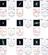 |
Fig. C.2. Fig. C.1 cont. |
| In the text | |
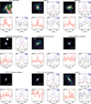 |
Fig. C.3. Fig. C.1 cont. |
| In the text | |
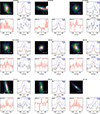 |
Fig. C.4. Fig. C.1 cont. |
| In the text | |
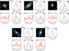 |
Fig. C.5. Fig. C.1 cont. |
| In the text | |
|
Fig. D.1. Targets observed with TNG/DOLORES. The image on the top left in each panel shows the SDSS r-band image of the target, with the size and position of the 3” SDSS fiber shown as a black and white dashed circle. The white bar in each image shows the size of the slit used in the TNG/DOLORES spectroscopy. On the top right in each panel we show the SDSS (on top in blue) and higher resolution TNG/DOLORES (below in black) spectra around the Hα emission line at 6562.8 Å, both converted to the same rest-frame velocity units. On the bottom right in each panel is the same plot for the [OIII] emission line at 5006.77 Å. For emission lines detected with S/N> 3 we also show the best fit model in red. If the model has multiple components, individual components are shown as dashed curves in green (non-outflow components) and orange (outflow components). On the bottom left is the region around the CO(1-0) or CO(2-1) emission line, whichever was used in the analysis, from the ALLSMOG and xCOLDGASS surveys. This figure is continued below in Fig. D.2. |
| In the text | |
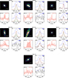 |
Fig. D.2. Fig. D.1 cont. |
| In the text | |
Current usage metrics show cumulative count of Article Views (full-text article views including HTML views, PDF and ePub downloads, according to the available data) and Abstracts Views on Vision4Press platform.
Data correspond to usage on the plateform after 2015. The current usage metrics is available 48-96 hours after online publication and is updated daily on week days.
Initial download of the metrics may take a while.