| Issue |
A&A
Volume 709, May 2026
|
|
|---|---|---|
| Article Number | A113 | |
| Number of page(s) | 12 | |
| Section | Planets, planetary systems, and small bodies | |
| DOI | https://doi.org/10.1051/0004-6361/202659026 | |
| Published online | 08 May 2026 | |
Numerical estimation of the capture ability of Neptunian mean motion resonances
1
State Key Laboratory of Lunar and Planetary Sciences, Macau University of Science and Technology,
Macau
999078,
China
2
School of Astronomy and Space Science, Nanjing University,
163 Xianlin Avenue,
Nanjing
210046,
China
3
Key Laboratory of Modern Astronomy and Astrophysics in Ministry of Education, Nanjing University,
China
★ Corresponding author: This email address is being protected from spambots. You need JavaScript enabled to view it.
Received:
19
January
2026
Accepted:
23
March
2026
Abstract
Resonant populations of trans-Neptunian objects serve as crucial dynamical archives for unraveling the early migratory history of the Solar System. A quantitative assessment of the capture efficiency into various mean motion resonances (MMRs) during migration is essential for understanding the origins of these populations, constraining migration parameters, and reconstructing of the primordial planetesimal disk. Using numerical simulations, this study systematically investigates the capture capability of exterior MMRs during Neptune’s outward migration in a planar model. For a specific p:q MMR, the small bodies can be captured only when their eccentricities surpass a certain threshold, emin, which increases with faster migration rates, greater distances of MMRs, and higher resonance orders. We also find that 1:q-type MMRs exhibit notably higher emin due to their unique dynamical structure. On the other hand, as long as a particle’s eccentricity is suitable, its capture efficiency shows little dependence on the migration rate; instead, it mainly depends on the p value and heliocentric distance, decaying exponentially as either parameter increases. Based on our simulation results, we derive for the first time a simple empirical expression to calculate emin and the capture efficiency. From beyond the 1:2 MMR out to approximately the 1:4 MMR, the theoretically predicted capture numbers follow a trend that resembles what is seen in observations, suggesting that migration capture could be the primary source of resonant populations in these regions. However, in more distant regions, the theoretical predictions fall significantly short of observational estimates, implying that other mechanisms (e.g., resonant sticking) might be necessary. This research provides a systematic quantitative framework for understanding capture into Neptunian MMRs during migration. Future integrations of more comprehensive observational data will facilitate a more precise reconstruction of the Solar System’s early dynamical evolution.
Key words: methods: numerical / celestial mechanics / Kuiper belt: general
© The Authors 2026
 Open Access article, published by EDP Sciences, under the terms of the Creative Commons Attribution License (https://creativecommons.org/licenses/by/4.0), which permits unrestricted use, distribution, and reproduction in any medium, provided the original work is properly cited.
This article is published in open access under the Subscribe to Open model. This email address is being protected from spambots. You need JavaScript enabled to view it. to support open access publication.
1 Introduction
Within the context of planetary migration, the distribution patterns of the vast majority of trans-Neptunian objects (TNOs) can now be explained (e.g., Levison et al. 2008; Morbidelli & Nesvorný 2020). Among these, Neptune’s mean motion resonances (MMRs) contain significant information about the early Solar System. As more TNOs are discovered, the insights embedded within Neptune’s MMRs, particularly those related to planetary migration, can be further elucidated.
Many mechanisms can influence both the number and distribution of small bodies within resonance belts. For instance, numerous studies have compared the stability of different MMRs (e.g., Morbidelli et al. 1995; Melita & Brunini 2000; Tiscareno & Malhotra 2009; Saillenfest et al. 2016; Li & Zhou 2024). This stability reflects the likelihood of objects escaping from MMRs after being captured. Other fundamental factors include the capture ability and capture locations of MMRs, which result in the distinct population sizes retained by different MMRs since the early Solar System.
A substantial number of prior studies have investigated the physical process of resonant capture. Early work often treated it as an adiabatic process, which required migration to be sufficiently slow, with a timescale that is significantly longer than the libration period of the resonant angle. Analytical methods have derived capture probabilities under idealized models (e.g., Peale 1976; Tiscareno & Malhotra 2009; Henrard 1982; Borderies & Goldreich 1984; Murray & Dermott 1999). A key conclusion of adiabatic capture theory is that when migration is sufficiently slow and the particle’s eccentricity is below a certain threshold, capture is inevitable. Conversely, if the particle’s eccentricity exceeds this threshold, the capture probability decreases progressively (Borderies & Goldreich 1984).
Wyatt (2003) further extended the study to higher migration rates, focusing on several specific MMRs and assuming a dynamically cold planetesimal disk. This work demonstrated that the capture probability increases with planetary mass and decreases with migration rates. Building on this, subsequent work employed Hamiltonian models to conduct a detailed exploration of first- and second-order MMRs, further investigating how different initial eccentricities of small bodies affect capture efficiency (Quillen 2006; Mustill & Wyatt 2011). These studies also systematically examined issues such as the interference of nearby resonant terms, the shifting of resonant centers during migration, the changes in eccentricity of particles upon failed capture, and the amplitude distribution of captured particles.
With advancements in technology and observations, resonant TNOs have been discovered in dozens of Neptunian MMRs, extending out to hundreds of astronomical units. Several studies have provided estimates of the number of objects within these resonant belts (e.g., Gladman et al. 2012; Volk et al. 2016; Crompvoets et al. 2022). Through direct numerical simulations within a planar model, we aim to test the ability of different Neptunian MMRs to capture bodies, quantify key parameters (e.g., the eccentricity threshold and probability for capture), and extend this analysis to higher order MMRs. Furthermore, we compare the predicted number of captured bodies in each MMR from our model with observational resonant populations, aiming to constrain the early dynamical evolution of the Solar System.
The remaining sections of this paper are organized as follows. In Section 2, we describe the numerical methods, the initial conditions, and the approach used to identify resonant objects. In Section 3, we analyze the simulation results, evaluate the capture capabilities of MMRs between 30 au to 80 au, carry out a detailed individual analysis of 1:q MMRs, and provide a comparison with observational estimates. Finally, we conclude with a summary and discussion.
2 Methods
2.1 Initial conditions
In this study, we employed a planar restricted three-body model consisting of the Sun, Neptune, and massless small bodies. Although other giant planets may significantly alter Neptune’s migration (e.g., Tsiganis et al. 2005; Nesvorný & Morbidelli 2012) and continue to affect the stability of MMRs after migration ends (e.g., Li & Zhou 2024; Graham & Volk 2024), this paper focuses solely on the physical process of capturing small bodies, which is predominantly governed by Neptune itself.
For a given p:q MMR (where p<q), its strength primarily depends on the resonance order k = q - p, with lower order MMRs generally exhibiting a greater strength. The nominal location of the MMR is given by aN × (p)2/3, where aN denotes Neptune’s semimajor axis. Under the simplified model considered in this paper, the resonant angle for an MMR can be expressed as φ = qλ - pλn - (q - p)ϖ, where λ and λn, respectively, represent the mean longitude of the small body and Neptune, while w represents the longitude of perihelion of the small body.
In each simulation, we applied an additional force in the direction of Neptune’s velocity, making Neptune migrate at a constant rate of ȧN. During this process, its eccentricity remains small and it can be considered on a circular orbit. Numerous previous studies have examined the influence of Neptune’s migration on resonance capture (e.g., Chiang & Jordan 2002; Li et al. 2014; Kaib & Sheppard 2016; Li & Zhou 2023). While there is no consensus yet on the precise details of Neptune’s migration, it is generally believed that during the early Solar System, a phase known as the giant planet instability occurred, during which the giant planets underwent dramatic orbital changes (see Nesvorný 2018, for a review). Therefore, we explored a wide range of ȧN values (from 0.01 au/Myr to 10 au/Myr), allowing each set of simulations to analogously represent MMR capture scenarios at different migration stages. In each simulation, the ȧN remains constant.
We first conducted a general statistical analysis of capture. In this setup, small bodies were distributed between 30 au and 80 au, with randomized semimajor axes. In other words, the surface density of the planetesimal disk is proportional to r−1, where r represents the heliocentric distance. The total number of particles is 50 000. In these simulations, Neptune migrates from 27 au to 30 au. The initial eccentricity e0 of the particles is randomly distributed between 0 and 0.35, while the angular elements, ϖ and M, are randomly distributed between 0° and 360°. For each MMR, we recorded the minimum initial eccentricity of the captured objects as emin and the number of objects captured into MMR as Pres.
Since we observed that 1:q MMRs required a higher emin to capture objects compared to other MMRs, we conducted an additional group of simulations focusing on this specific category. In these simulations, Neptune migrates from 29 au to 30 au and the semimajor axes of the planetesimals are set to the nominal resonance location corresponding to Neptune at 29.5 au (i.e., 29.5 × q2/3). In this simulation set, 180 w values were sampled uniformly from 0° to 358° and M was fixed at 0°. Additionally, we tested multiple sets of different e0 until the value of emin could be determined within a precision of one-thousandth.
The integrations in this study are performed using the N-body code REBOUND (Rein & Liu 2012), employing the WHFast algorithm, a Wisdom-Holman symplectic integrator (Rein & Tamayo 2015; Wisdom & Holman 1991). Depending on the values of ȧN and the total migration distance, the duration of Neptune’s migration varied, while in all cases it stops upon reaching 30 au. After this phase, the additional force driving migration is removed and each simulation is extended for another 0.5 Myr, with relatively frequent output intervals to determine whether each object is within the MMR.
2.2 Resonator identification
Following the simulation setup described in the previous subsection, we first determined whether the particles reside within MMRs. Traditionally, this would require assessing whether their resonant angle is in libration. However, in this simulation, we did not know in advance whether a given particle was in MMR or which specific MMR it might occupy. Therefore, we adopted a semimajor axis-based method to make this determination. To this end, we denoted the particle’s initial and final semimajor axis as ai and af, respectively. The mean semimajor axis during the final 0.5 Myr of the simulation, when Neptune no longer migrates, was recorded as a. In Fig. 1, we illustrate the process of identifying resonant objects, using the simulation with ȧN = 0.2 au/Myr as an example. As shown in the upper panel of Fig. 1, the a value of small bodies exhibits clear clustering at MMR locations, which are marked by horizontal dashed lines. This clustering served as the key basis for identifying resonators.
If a particle is captured by an MMR and migrates outward with Neptune, its orbit also expands accordingly. Based on their ai and a, we first filtered particles captured by Neptune during the first 90% of its migration path. This requires the particle to have been captured before Neptune reaches 29.7 au, namely, satisfying  . Additionally, we excluded particles with eccentricities greater than 0.45, as well as those whose semimajor axis varied by more than 2 au during the final 0.5 Myr.
This filter excludes the following three types of particles: (1) particles that experience minimal resonant influence; their semimajor axes remain almost unchanged or slightly reduced, resulting from MMRs crossing without being captured (Mustill & Wyatt 2011). These particles generally have relatively low eccentricities and are distributed approximately along the diagonal from the lower left to the upper right in Fig. 1; (2) particles captured during the final 10% of Neptune’s migration path. In our model, Neptune migrates outward at a constant rate and stops abruptly upon reaching 30 au. As noted by Li & Zhou (2023), in such cases, the final capture scenarios are different from those during the migration, due to the deceleration or stopping of migration. Therefore, we excluded those particles when statistically analyzing resonant objects. This filtering step treats different MMRs fairly and does not impact the comparisons between them. This category of particles, as with other resonant bodies, is also located near the MMR positions shown in Fig. 1; and (3) objects that primarily belong to the scattered disk and usually have a lower perihelion distance. Due to their significant variations in semimajor axis during the final 0.5 Myr, their positions are primarily located far from the diagonal region in Fig. 1.
Since resonant objects oscillate around the nominal resonance location, their a are very close to the nominal value, typically with a deviation of less than 0.01 au, as illustrated in the lower panel of Fig. 1. Accordingly, we group particles based on their a, with each group representing an MMR or, in a few cases, isolated particles not captured into any MMRs. We further excluded groups with less than 10 particles, ensuring that nonresonant particles were filtered out and eliminating MMRs with few members. In the example shown in Fig. 1, several high-order MMRs (e.g., 13:22, 10:17,11:19, and 11:20) were excluded due to an insufficient number of particles. This step is reasonable as we need to statistically assess emin and Pres for each MMR; groups with too few particles would lack statistical significance, and the derived emin could deviate substantially from the true value.
To validate the accuracy of this resonator identification method, we also checked the resonant angles of all small bodies near the 4:7 MMR. Objects with librating resonant angles are shown in the lower panel of Fig. 2, with colors indicating their libration amplitudes of resonant angle. We found that all small bodies selected by the aforementioned method exhibit librating resonance angles, confirming the effectiveness of the approach. For some objects, while their resonant angles were librating, they were excluded due to insufficient semimajor axis increment. These objects were captured during the final 10% of Neptune’s migration and located at the edge of the resonance island, resulting in larger libration amplitudes.
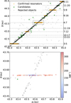 |
Fig. 1 Resonance identification procedure based on semimajor axis. The horizontal axis represents the final semimajor axis, af, of the particles, while the vertical axis represents their mean semimajor axis, a, during the final 0.5 Myr. The figure shows the region near the 4:7 MMR in the simulation with ȧN = 0.2 au/Myr. In the upper panel, black crosses indicate objects excluded during the initial filtering, green crosses represent resonant candidates that were subsequently excluded during clustering, and orange dots denote particles finally identified as resonators. Horizontal dashed lines mark the positions of several MMRs. The lower panel provides a magnified view of the dotted rectangular region in the upper panel, where all particles residing in the 4:7 MMR are identified based on the libration of their resonant angles, with colors indicating the corresponding libration amplitudes. |
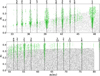 |
Fig. 2 Distribution of final semimajor axis, af, and final eccentricity, ef, from simulations with ȧN = 0.2 au/Myr. Green points represent objects identified as being in MMRs, while the gray points indicate the others. The positions of some major MMRs are marked with dashed lines, with the corresponding p (upper number) and q (lower number) values indicated above the lines. For clarity, the figure is divided into two panels using 49 au as the boundary, showing the inner and outer regions separately. |
3 Results
In this section, we present the simulation results and our understanding the capturing capacity of each MMR. This not only validates previous theories of resonant capture (Borderies & Goldreich 1984; Wyatt 2003; Quillen 2006; Mustill & Wyatt 2011), but also extends these theories to higher order MMRs. As an example, Fig. 2 illustrates the simulation results when ȧN = 0.2 au/Myr.
In Fig. 2, the vertical band-like structures in green can be observed, each corresponding to an MMR. It is evident that the majority of resonant objects are concentrated in the inner region. Within 50 au, even the ones that have not been captured by MMR have had their orbits significantly modified, either by Neptune’s scattering or MMRs’ sweeping. Beyond 60 au, the influential MMRs become relatively sparser and the number of resonant objects decreases significantly. Meanwhile, particles that were not captured largely remained near their initial positions and experienced limited influence from the MMR sweeping. Furthermore, Fig. 2 illustrates that stronger resonances exhibit broader resonance widths and are able to capture small bodies at lower eccentricities, a phenomenon we discussed in detail later in this paper.
We conducted eight simulations with different ȧN values and observed 74 MMRs that captured more than ten particles in at least one simulation. Among the outermost MMRs, we retained the 2:9 MMR located near 81.8 au (visible on the far right of Fig. 2), as its swept area predominantly lies within 80 au. The 3:14 MMR and the 1:5 MMR were excluded, despite also capturing a number of objects. To minimize the influence of randomness, we selected 66 MMRs that captured more than 10 particles in at least two simulations. The highest order MMR among these is the 9:25 MMR at 59.3 au, whose order is 16. For these MMRs, we computed their emin and Pres , summarizing the results in Fig. 3.
In most cases, capture occurs only when the eccentricity of the small body exceeds a certain threshold, corroborating previous findings by Mustill & Wyatt (e.g. 2011). Some patterns can be directly observed in Fig. 3. For example, higher order MMRs generally require a higher emin compared to lower order MMRs, and a faster ȧN also raises this threshold. On the other hand, the Pres varies significantly among different MMRs, while is relatively insensitive to the ȧN. Nevertheless, for certain MMRs (e.g., the 1:3 MMR), Pres decreases notably as ȧN increases. The main reason is that the emin increases with faster ȧN. As a result, the number of particles eligible for capture correspondingly decreases. In the following, we discuss the variations of emin and Pres across different MMRs and a range of ȧN.
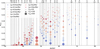 |
Fig. 3 emin and Pres for different MMRs under various ȧN values. The horizontal axis represents the final location of each MMR, the vertical axis shows the minimum initial eccentricity, emin, for each MMR, the color of the points indicates Neptune’s migration rate ȧN in the simulation, and the size of the points represents the number of captured small bodies, Pres. Some of the major MMRs are marked with dashed black lines, with their corresponding p and q values indicated above the lines, while other MMRs are shown with gray dashed lines. |
3.1 Minimum eccentricity for MMR capture
To discuss the distribution of emin across different ȧN and MMRs, we first need to identify those MMRs capable of capturing small bodies even when they are in circular orbits. Therefore, we defined that if a MMR has an emin smaller than 0.005, it is considered capable of capturing objects at e0 = 0. The method used to initialize the small bodies ensures that there are approximately 1000 small bodies per astronomical unit, of which about 14 have e0 < 0.005. Since Neptune migrates over a distance of 3 au, an exterior MMR necessarily sweeps through a distance greater than 3 au. Therefore, each MMR would have encountered at least several dozen objects with e0 < 0.005.
First, we focus on the first-order MMRs separately, as they typically exhibit efficient capture down to zero initial eccentricity. Our statistics included six first-order MMRs, from the 1:2 MMR to the 6:7 MMR, as shown in Fig. 3. The 1:2 MMR can capture objects with e0 = 0 only when ȧN ≤ 1 au/Myr, whereas other first-order MMRs can do so under any ȧN up to 10 au/Myr. This is likely related to the fact that first-order MMRs retain a certain degree of resonance width even as eccentricity approaches zero (e.g., Murray & Dermott 1999; Morbidelli 2002). In addition to these six first-order MMRs, three second-order MMRs and one third-order MMR are also capable of capturing particles with e0 = 0 under sufficiently slow migration: the 3:5 MMR (ȧN ≤ 0.2 au/Myr), the 5:7 MMR (ȧN ≤ 1 au/Myr), the 7:9 MMR (ȧN ≤ 2 au/Myr), as well as the 7:10 MMR (ȧN ≤ 0.01 au/Myr).
For the remaining cases, by comparing different MMRs of the same order under identical ȧN, it can be observed that MMRs located farther away require a larger emin values. To standardize the capture performance of MMRs at varying distances, we first recalibrated the obtained emin. To this end, we denote the ratio of the MMR’s nominal semimajor axis to that of Neptune as  , finding that the value of
  remains roughly consistent across different positions for the same order of MMRs. The reciprocal of the coefficient
  also carries physical significance: when the eccentricity of a small body reaches
  , its perihelion reaches the orbit of Neptune. For convenience, we hereafter refer to
  as the critical eccentricity, denoted as ec.
Following the recalibration, we examined the new quantity  . In Fig. 4, we present the relationship between
  and the resonance order, k, under different ȧN. We observe that
  essentially follows a linear relationship with the resonance order, k.
Moreover, we note that if linear fitting is applied to describe the relationship between  and k at different ȧN, the fitted lines roughly converge at a common point. Although this property may not hold any direct physical significance, it allows us to characterize the variation of
  using a simpler function. Through fitting, we express the relationship between
  , the resonance order, k, and the migration rate, ȧN, as follows:
 (1)
(1)
In Eq. (1), the function f (ȧN) depends on the ȧN and reflects how the slope of the aforementioned linear relationship increases with increasing ȧN. A subsequent fitting indicates that the f (ȧN) is well approximated by an exponential function, namely,
 (2)
(2)
In Fig. 4, we also present the fitting results for different ȧN values based on Eqs. (1) and (2), represented by lines in corresponding
colors. Despite their relatively simple forms, Eqs. (1) and (2) still provide a satisfactory estimation. They effectively capture the phenomenon that as the k or ȧN increases, the value of  also rises correspondingly. The fitting remains robust even under conditions of rapid migration or high resonant orders, yielding a coefficient of determination of R2 = 0.97.
In our simulations, six MMRs were identified with more than ten objects in the slowest simulation only, with ȧN = 0.01 au/Myr: 10:19, 8:25, 7:24, 5:19, 4:17, and 3:14 MMRs. With the exception of the 10:19 MMR, which is relatively close, all of them are located beyond the 1:3 MMR. These MMRs are not plotted in Fig. 3 and their emin values were not included in the fitting for Eqs. (1) and (2). Here, we used them as a validation set, marking them with purple square symbols in Fig. 4. It can be seen that their positions still lie approximately along the fitted purple line, demonstrating the validity of Eqs. (1) and (2).
However, two issues warrant attention. First, Eqs. (1) and (2) provide only a qualitative description of the variation pattern of emin and their functional forms do not carry any corresponding physical significance. In particular, the origin data used for fitting were derived from numerical simulations and represent only an approximate value, serving as an upper limit on the true emin. Since the true emin should be more or less smaller, the fitting results shown in Fig. 4 likely overestimate emin to some extent.
For example, based on Eqs. (1) and (2), it can be inferred that as the migration rate ȧN approaches 0, we obtain  . This expression becomes nearly zero when k = 5. Therefore, it can be deduced that no matter how slow Neptune’s migration, those high-order MMRs with k ≥ 6 are incapable of capturing small bodies with e0 = 0. However, given that this fitting serves as an upper estimate for the true emin (which is likely slightly lower), further research and validation are necessary to confirm whether this conjecture is merely an artifact of the model or reflects a genuine dynamical characteristic.
Another issue is that Eqs. (1) and (2) exhibit significant deviation in predicting 1:q-type MMRs. In the above simulations, three 1:q MMRs from 1:2 to 1:4 were identified, which have been marked with cross symbols in Fig. 4. However, it can be observed that all 1:q MMRs consistently exhibit a higher emin than predicted. Therefore, we excluded these three 1:q MMRs from the fitting process described earlier. The most prominent characteristic of 1:q MMRs is that they are the farthest among MMRs of the same order. Previously, we introduced ec to correct for the influence of resonance distance and find that, with the same k and ȧN, the value of  is similar. Although this correction is empirical, it aligns well for cases where p ≥ 2.
Compared to other MMRs, another major distinction of 1:q MMRs lies in their intrinsic resonance structure, as their resonance islands contain two asymmetric libration centers; namely, leading and trailing centers (e.g., Message 1958; Frangakis 1973; Beauge 1994; Malhotra 1996; Kotoulas 2005; Voyatzis et al. 2005). Furthermore, Neptune’s migration can distort the phase-space structure of MMRs, breaking the symmetry between the leading and trailing islands (Chiang & Jordan 2002; Murray-Clay & Chiang 2005; Li & Zhou 2023). This complex structure may be the reason why 1:q MMRs require a relatively higher emin to capture small bodies.
Given that there are only three 1: q MMRs within 80 au, we conducted a dedicated set of simulations specifically targeting 1:q MMRs to determine their emin. In this set of simulations, we employed a relatively uniform selection method for particles to achieve more accurate results (as detailed in Section 2). We expanded our study to include the 1:9 MMR, which has recently been identified to have two resonators, suggesting a potentially large population size (Volk et al. 2018; Crompvoets et al. 2022).
When we focus specifically on 1:q MMRs, parameters such as the corresponding k and α can be directly determined once q is specified. Therefore, we can adopt a simpler functional form. We eliminated the correction based on ec and directly fitted the variation pattern of emin using a expression similar to that given Eqs. (1) and (2), while reducing one parameter (the constant term in Eq. (2)). Through fitting, we obtain that the emin for 1:q MMRs can be approximately expressed by the following empirical formula,
 (3)
(3)
In Fig. 5, we display the distribution of  for 1:q MMRs, along with the fitting results using Eq. (3). As a result of the more accurate and equitable determination of
  in this simulation set, the fitting performance provided by Eq. (3) is more robust, achieving a coefficient of determination of 0.99.
After deriving Eq. (3), we can roughly compare its predictions with those of Eqs. (1) and (2). For q = 2, both formulations predict an emin close to zero. However, for cases where q ≥ 3, if the fitting results derived from non-1:q MMRs are arbitrarily applied to 1:q MMRs, the values given by Eqs. (1) and (2) are, on average, lower by 0.15 compared to the “true values” provided by Eq. (3). In other words, a relative deviation of approximately 40%, highlighting the distinctly different behaviors of emin for 1:q MMRs compared to non-1:q MMRs.
As detailed in Section 2.1, our simulations have covered most migration rates, resonance orders, and semimajor axis ranges of practical interest. Eqs. (1), (2), and (3) are empirical formulas obtained by fitting within this parameter space. However, it is important to note, based on their functional forms alone, that Eqs. (1) and (3) can both predict emin > 1 under very fast ȧN and/or very high k, which is clearly unphysical. In fact, indications of this limitation can already be seen from Fig. 5: when the  (emin ≳ 0.6), the data points no longer closely follow the linear trend, but mostly fall below the fitted line. This suggests that the fits provided by Eqs. (1) and (3) are likely more effective in the low-to-moderate eccentricity regime and require further refinement for extremely high eccentricities. In other words, caution is advised when applying these fitting formulas under conditions of extremely fast migration and high resonance orders.
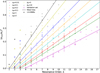 |
Fig. 4 Relationship between |


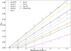 |
Fig. 5 Relationship between |


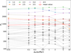 |
Fig. 6 Variation in the capture efficiency of MMRs under different ȧN. The horizontal axis represents the migration rate, ȧN, and the vertical axis represents the capture number per unit eccentricity, Pe, both on logarithmic scales. The seven MMRs with the strongest capture capability are denoted by colored lines, while the others are shown in gray. The average result across all MMRs is represented by the solid red line with triangular markers. |
3.2 Efficiency of MMR capture
Compared to the emin of MMRs, the question of how many small bodies an MMR can capture is more complex. One key consideration is that as ȧN increases, emin gradually rises as well, which reduces the number of small bodies suitable for capture. Additionally, when Neptune approaches, if the perihelion of a small body is too close to Neptune, it might get scattered away before resonant capture can occur. Therefore, we imposed an upper eccentricity limit emax, defined such that the perihelion of an object can reach within 32 au (i.e.,  ). Small bodies with initial eccentricities exceeding emax are not counted in our statistics. Captures in this regime are rare and do not result purely from Neptune’s migration; instead, they involve either eccentricity damping through resonance crossing prior to capture or being initially placed inside the MMRs. For more distant MMRs (where emax > 0.35), the eccentricity upper limit is set by a maximum eccentricity of 0.35 defined in the simulations.
To compare the capture capabilities of MMRs under different ȧN, we first corrected for the decrease in Pres caused by the increase in emin. Thus, we define the “capture number per unit eccentricity,”  , to describe the capture efficiency of an MMR within the eccentricity interval suitable for capture. Based on the previous subsection, we selected 33 MMRs that captured more than ten particles in all eight simulations and calculated their Pe, as presented in Fig. 6.
As can be seen in Fig. 6, the lines corresponding to each MMR generally exhibit a horizontal trend, indicating that after correction, Pe is no longer significantly correlated with ȧN, but mainly related to the intrinsic capture capability of the MMR itself. The average relative standard deviation is about 13.8%, whereas the relative standard deviation for the average capture number across all MMRs is only 3.0%. The most efficient MMRs (e.g., the 1:2, 2:3, and 3:4 MMRs) show robust capture across a wide range of ȧN. The Pres result from the 2:3 MMR provides the most direct evidence that Pe and ȧN are unrelated, as its emin is always 0, meaning the suitable eccentricity range remains unchanged. Across eight different ȧN values, the 2:3 MMR captures an average of 817 objects, with a standard deviation of only 48.
Nevertheless, a certain degree of fluctuation still exists, which may primarily be attributed to randomness. As a result, this fluctuation slightly increases as the Pe decreases. The deviations in the estimation of emin might also contribute to an increase in overall fluctuations. However, the amplitude of these fluctuations typically does not exceed 100%, which is far less than the differences between MMRs. Furthermore, a few MMRs also exhibit specific trends; for instance, as ȧN increases from 0.01 to 10 au/Myr, the Pe for the 1:3 MMR decreases from 1731 to 647, while for the 4:5 MMR, it increases from 1362 to 2838. These specific trends may be due to more complex reasons, such as the interference between different MMRs.
Next, we assume there is no significant correlation between the Pe and the migration rate, or at least, that any such correlation is considerably smaller than the differences between different MMRs. Therefore, an average Pe, denoted as Pe, can be used to characterize the capture ability of an MMR. By comparing the Pe values for different MMRs, we find that a simple exponential expression can be utilized to estimate the Pe value,
 (4)
(4)
The coefficients in Eq. (4) are derived by fitting the data from the aforementioned 33 MMRs that captured over ten particles in all simulations. This expression indicates that the capture capability of an MMR decreases as the p value increases and as the distance becomes greater. Figure 7 illustrates the fitting performance of Eq. (4).
Figure 7 displays a good fitting result with a coefficient of determination of R2 = 0.95. As a test, we also calculated the Pe for MMRs that had capture records in only some simulations. These results are displayed in Fig. 7 using markers without borders and the Pe of these MMRs can still be aptly predicted by Eq. (4). There are several MMRs with relatively small Pe; the simulation values often exceed the predicted values, which is likely attributed to a selection effect inherent in the data processing method. Since these MMRs are only recorded when the capture count exceeds 10, there is a systematic overestimation of their capture capabilities.
A particularly intriguing observation is that only the p value and α appear directly in Eq. (4), with no direct inclusion of the q value or the resonance order, k. In practice, during the fitting process, we also experimented with other parameter combinations, such as any two of α, p, q, and k. We find that the combination of p and α yields a significantly better fit compared to other parameter combinations. When using three parameters simultaneously (e.g., α, p and q), the improvement in the R2 was only marginal. Therefore, after careful consideration, we conclude that using only p and α is sufficient to effectively describe the variation in Pe across different MMRs.
A plausible explanation is that for a fixed p, increasing q results in a higher resonance order, but simultaneously, it also expands the range swept by the resonance zone. These two effects may counterbalance each other, leading to minimal changes in capture efficiency. On the other hand, the importance of p lies in the fact that MMRs with lower p values are spaced farther apart from each other, reducing mutual interference.
In Eq. (4), we see that q indirectly influences Pe by affecting the parameter α. When the p value is small (p ≲ 4), α increases rapidly as q increases, leading to a noticeable decrease in Pe and resulting in relatively large differences in capture capability among MMRs with the same p value. Conversely, when the p value is relatively large (p ≳ 5), a slight increase in the q value does not cause significant change in α. In this case, the capture capabilities of different MMRs are similar, which facilitates the comparison of capture capabilities among high-p MMRs. For example, the Pe values for the 5:11, 5:12, 5:13, and 5:14 MMRs are 491, 532, 480, and 460, respectively.
It should be noted that due to the application of a series of data processing methods, the metric Pe used here has undergone multiple conversions. Because the absolute number of particles that an MMR can capture also depends on the specific design of the model, involving factors such as Neptune’s migration distance, and the spatial and size distributions of small bodies, the focus often lies on the ratios between their numbers (e.g., Crompvoets et al. 2022). This pertains to the relative magnitudes of Pe across different MMRs. The coefficient 49 316 in Eq. (4) is not a critically important value in itself, as its magnitude primarily depends on artificial settings, particularly the particle number used in the simulation.
In addition to its usefulness in comparisons between different MMRs, the metric Pe can also be directly applied to calculate the capture probability of a given MMR. In the planetesimal disk considered in this work, there are approximately 1000 small bodies per astronomical unit. Therefore, for every astronomical unit Neptune migrates, the region swept by an MMR contains roughly 1000α small bodies. When extended to the unit eccentricity, the density will be approximately  objects per astronomical unit. If we further assume that all particles lie within the eccentricity range suitable for capture, then the number of particles captured per astronomical unit of Neptune’s migration should be approximately
  (Neptune migrates a total of 3 au, but we only count particles captured during the first 90% of its migration). This leads to the conclusion that for a particle with an appropriate eccentricity, the probability of being captured by that MMR is approximately
  .
.
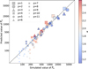 |
Fig. 7 Distribution of the average capture capability, Pe, across different MMRs. The horizontal axis represents the measured Pe from simulation data, while the vertical axis represents the Pe predicted by Eq. (4), both on logarithmic scales. MMRs with different p values are denoted by different markers and the color indicates the α value of the MMR. Points with black borders are the MMRs that have capture records in all simulations, while those without borders are the MMRs have capture records in only some of the simulations. |
3.3 Comparison with observations
Thus far, we have established that the emin required for capture by an MMR increases as its distance becomes greater, its order increases, and the migration accelerates. The number of objects captured by an MMR first depends on the eccentricity range over which resonant capture can occur. As the ȧN increases, the rise in emin narrows this eccentricity range, resulting in a corresponding decrease in the capture number. After correcting for the change in capture number caused by variations in emin, the Pe of an MMR shows little correlation with the ȧN. Hence, it can be characterized by Pe, whose value decays exponentially with increasing p and α. In this subsection, we examine several simple Neptune migration models to calculate the resonant populations captured by different MMRs, and compare them with observational estimation.
Several previous studies have provided estimates of the population sizes of MMRs, with some offering comparisons among different MMRs (e.g., Gladman et al. 2012; Adams et al. 2014; Volk et al. 2016; Crompvoets et al. 2022). Other studies have focused on specific MMRs (e.g., Pike et al. 2015; Alexandersen et al. 2016; Volk et al. 2018; Chen et al. 2019). Building upon these works, we summarize MMRs with available estimates of population size in Table 1. For certain MMRs (e.g., 2:3, 1:2, 2:5, 1:5), the various estimates available from the literature demonstrate a good degree of consistency. In Table 1, we have preferentially adopted the most recent estimates.
Overall, based on the current sample sizes of observed resonant TNOs, only a few MMRs such as the 2:3, 1:2, and 2:5 MMRs have relatively well-estimated population sizes. Most MMRs have sparse observations, providing only rough estimates in terms of order of magnitude. This means that a precise comparison between observational results and theoretical predictions is premature at this stage. Among all MMRs, the population in the 2:3 MMR is the most accurately determined. In this paper, we use this MMR as a benchmark to compare the relative population differences of other MMRs against it.
Based on the resonance capture laws derived in the previous two subsections, we can calculate the number of particles captured by a given MMR in two steps. Firstly, for a given distribution of particles, we calculate how many particles within the region swept by the MMR fall into the range suitable for capture. This calculation involves Neptune’s initial and final positions, as well as the number density of particles across different eccentricities and semimajor axes. Since the aim of this study is a rough comparison, we assume a uniform semimajor axis distribution, where the surface density of the planetesimal disk is proportional to r−1, so that the ratio among different MMRs becomes independent of the specific migration start and end points of Neptune.
We further assume a Rayleigh distribution for eccentricity, which has been shown to be an effective description for main belt asteroids (see e.g., Plummer 1916; Beck 1981; Malhotra & Wang 2017; Liu et al. 2023). Under the above assumption, the number of bodies suitable for capture is proportional to r-1, where emin is given by Eq. (1) (for non-1:q MMRs) or Eq. (3) (for 1:q MMRs),  , and σe denotes the parameter of the Rayleigh distribution. Multiplying the number of particles by the probability of capturing a particle with an appropriate eccentricity,
  , we can obtain the number of captured objects by a specific MMR as provided in the previous subsection,
 (5)
(5)
Under this idealized model, the entire calculation of Eq. (5) involves only two parameters: σe, which describes the level of eccentricity excitation of particles, and ȧN, which describes the migration rate. For this calculation, we scaled all Pres values by a uniform factor so that Pres for the 2:3 MMR matches the observed value of 10000. Selecting the 2:3 MMR as a reference standard is due to its largest observed population and the most robust population estimate, as well as its superior capture ability, which remains unaffected by the migration rate (as shown by Fig. 6). We selected three different σe values: 0.1, 0.2, and 0.3, corresponding to average eccentricities of 0.125, 0.251, and 0.376, respectively. Four different ȧN values were tested, ranging from 0.01 au/Myr to 10 au/Myr. Fig. 8 illustrates the results obtained using these different parameters and compares them against the observational values.
Regarding the influence of the eccentricity excitation of the planetesimals, most MMRs tend to obtain a larger Pres in a disk with a higher σe. This does not indicate a higher capture probability for individual planetesimals at high eccentricity, but rather reflects that the vast majority of particles in a dynamically cold disk are unsuitable for capture. However, for the two innermost MMRs, 3:4 and 4:5, this trend is reversed because they only exhibit good capture capability at lower eccentricities, compared to the 2:3 MMR. On the other hand, the effect of the migration rate is indirect: it alters the captured population by influencing emin. This effect is particularly pronounced when σe = 0.1, because the variation in emin induced by ȧN can significantly alter the number of particles suitable for capture, potentially leading to an order-of-magnitude change in Pres.
For MMRs interior to the 1:2 MMR, the Pres is relatively less sensitive to the parameters. In particular, the Pres for the 3:4 and 4:5 MMRs are solely dependent on σe and not on ȧN, making their observational values a crucial information. Within this region, all theoretical predictions are higher than the observations. For the nearer 3:4 and 4:5 MMRs, the population estimates still carry large uncertainties due to the limited sample sizes. However, no parameter combination yields theoretical values within the confidence interval of the observations. This discrepancy reflects a significant overestimation of Pres for the 3:4 and 4:5 MMRs by the assumptions used in this study. On one hand, compared to the 2:3 MMR, the particles in the 3:4 and 4:5 MMRs may be significantly less stable due to their proximity to Neptune (e.g., Kotoulas & Voyatzis 2004). On the other hand, these inner regions might have been unfavorable for planetesimal growth during the formation of the giant planets, leading to a sparser population of planetesimals.
Another MMR with a notably higher prediction is the 1:2 MMR. Current observations suggest that the population in the 1:2 MMR is only about half that of the 2:3 MMR, but simulations show that their populations are at least comparable. The primary reason for this discrepancy lies in the poorer stability of the 1:2 MMR. Melita & Brunini (2000) pointed out that compared to the 2:3 MMR, the resonant islands of the 1:2 MMR are more fragmented, especially at low inclinations, which should prevent it from hosting a large population of bodies. Through frequency analysis of the 1:2 and 1:3 MMRs, Li & Zhou (2024) also found that the latter exhibits a cleaner dynamical map and longer dynamical stability timescales, attributed to its greater distance and slower eigenfrequency. A similar phenomenon is observed for the 3:5 and 4:7 MMRs, whose predicted values are slightly higher than the observations (though still within the error margins). If observational errors are excluded, this might simply be due to the slightly poorer stability of these two MMRs compared to the 2:3 MMR (e.g., Melita & Brunini 2000).
In the region beyond the 1:2 MMR, extending up to around the 1:4 MMR, we note that the observed populations for most MMRs in this range agree with the theoretical Pres at least in order of magnitude and exhibit nearly identical trends. This suggests a high probability that the small bodies within these MMRs were captured by Neptune through migration, leading to several indirect inferences: Firstly, the primordial planetesimal disk potentially extended to around 60 to 70 au, maintaining a relatively flat distribution without a sharp density drop-off. Secondly, these MMRs likely possess good long-term stability due to their greater distances, suggesting that their ability to retain objects is comparable to that of the 2:3 MMR. Thirdly, the scenario of rapid migration (ȧN ≥ 1 au/Myr), combined with a dynamically cold planetesimal disk (σe = 0.1) can be ruled out, as under such conditions, the vast majority of small bodies would fail to meet the condition e ≥ emin.
The situation becomes more complex for more distant MMRs, and the most prominent issue is the further increase in observational uncertainties. In this region, theoretical predictions are generally lower than the observational estimates. This discrepancy may partly stem from randomness, as the extreme distance means that even a few sporadic detections can lead to large population estimates. Meanwhile, many other MMRs in this region, such as the 1:6 MMR, are currently lacking observational data.
Moreover, at such remote locations, the primary mechanism for supplementing resonant bodies might be the resonant sticking effect, and these existing bodies may not constitute the primordial population captured by Neptune’s migration but are only temporarily trapped within these MMRs (Yu et al. 2018). Crompvoets et al. (2022) have also noted that predictions based on resonant sticking effects align better with observations than migration models. Overall, however, explaining the existence of a large population in such distant regions remains challenging, necessitating more observational samples and higher resolution simulations in the future.
In more realistic models of the Solar System, Neptune is often considered to have undergone migration following an exponential decay pattern, a model commonly referred to as the exponential migration model (e.g., Malhotra 1995). Subsequently, it was proposed that Neptune’s migration was not smooth but rather grainy (Nesvorný & Vokrouhlicky 2016; Lawler et al. 2019), and may even have involved a major jumping (Nesvorný & Morbidelli 2012; Nesvorný 2015). So far, we have established a method for calculating capture into Neptune’s MMRs under a constant migration rate. This method can be readily extended to scenarios where the migration rate varies. Here, we adopt a simple exponential migration model as an illustrative example.
In an exponential migration model, Neptune starts from aNi and finally stops at aNf. The evolution of Neptune’s semimajor axis can be expressed as  , where τ is the migration timescale. The migration rate ȧN can then be written as a function of semimajor axis, namely
  . Therefore, the average migration rate is easily obtained as
  . it should be noted that this average is taken over different semimajor axes, not over time. On the other hand, the captured number by a specific MMR can be obtained by integrating over different semimajor axes, namely,
 (6)
(6)
Generally, Eq. (6) would also need to account for the possibility that the planetesimal density and σe are functions of semimajor axis. However, under our assumptions, the planetesimals follow a uniform semimajor axis distribution and a consistent eccentricity excitation, and both emax and Pe in Eq. (6) are also unaffected by ȧN. Consequently, the only quantity in Eq. (6) that depends on aN is emin.
As a test case, we assumed aNi = 25 au, aNf = 30 au, and τ = 25 Myr. Under different σe, we calculated the capture capability of various MMRs within this exponential migration model and marked them with cross symbols in Fig. 8. Since the average migration rate for this model is 0.1 au/Myr, we can conveniently compare this exponential migration model with the linear migration model for ȧN = 0.1 au/Myr.
As shown in Fig. 8, the results from all cross symbols and square symbols are nearly consistent. Examining cases where Pres > 1, the maximum difference introduced by the exponential model occurs for the 1:5 MMR and σe = 0.1, where the Pres obtained from the exponential migration is twice that of the constant migration with ȧN = 0.1 au/Myr. This difference arises because 1:q MMRs have a larger capture efficiency, but also a relatively higher emin. Consequently, the slow phase at the end of exponential migration makes a substantial contribution to their total captured population. Aside from this particular case, the average difference between the exponential and constant migration models is only 4.3%. This minor difference is nearly indistinguishable when plotted on the logarithmic scale of Fig. 8. Particularly given that current comparisons with observations are only at the order-of-magnitude level, exponential and constant migration models exhibit virtually no difference when their average migration rates are the same.
Estimated numbers of objects in various MMRs provided by previous observational works.
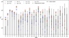 |
Fig. 8 Captured population for each MMR under different parameters, compared with observations. The histogram displays the current observational results, with error bars indicating observational uncertainties (details in Table 1). Different markers denote different migration rates, while the crosses specifically denote the exponential migration model with an average migration rate of 0.1 au/Myr. Different colors represent different eccentricity excitations for the small bodies. The x-axis provides the corresponding p (above) and q (below) values for each MMR, arranged at equal intervals in order of proximity. The y-axis represents the population within each MMR, all data are normalized, with the 2:3 MMR as a reference standard. |
4 Conclusion and discussion
In this paper, we systematically investigate the ability of Neptune’s exterior MMRs to capture objects and provide a detailed numerical assessment. Based on previous theories of resonance capture (e.g., Mustill & Wyatt 2011), a specific MMR under a given migration rate can only capture small bodies with eccentricities exceeding a certain threshold, termed the minimum capture eccentricity, emin. Depending on the capture efficiency of each MMR, the number of captured small bodies Pres varies. We first employed a simple model to identify particles captured by MMRs (as shown in Figs. 1 and 2) and determined their corresponding emin and Pres under different migration rates (Fig. 3).
Then we fit emin and Pres using simple functional expressions. Following the appropriate scaling, the  of MMRs roughly follows a linear relationship with their resonance order and the slope of this line can be expressed as a function of Neptune’s migration rate ȧN (Eqs. (1) and (2) and Fig. 4). Meanwhile, the pattern followed by 1:q MMRs shows some differences, their emin are significantly higher than those of non-1:q MMRs (Eq. (3) and Fig. 5). This suggests that the unique dynamical structure of 1:q MMRs may differentiate them from other MMRs, making them capture only small bodies with relatively higher eccentricities.
As for Pres, the primary conclusion is that ȧN directly influences only emin, thereby indirectly affecting Pres, while the capture efficiency per unit eccentricity, Pe, is almost unaffected by ȧN (Fig. 6). This character leads us to use Pe to describe the probability of capturing objects. Through fitting, we find that Pe can also be expressed with a simple formula: it decays exponentially with increasing p value and α value of the MMR (Eq. (4) and Fig. 7).
In this step, we made a major assumption that MMRs capture objects with roughly uniform probability within the suitable eccentricity range (from emin to emax), whereas in reality this is not the case. Previous works have found that at a given migration rate, the probability of an MMR capturing a small body transitions from near certainty to near impossibility as eccentricity increases. Furthermore, for second-order MMRs, this transition occurs over a broader eccentricity range compared to first-order MMRs. (e.g., Mustill & Wyatt 2011). Therefore, it is reasonable to speculate that the assumption of the capture probability being independent of eccentricity may only be approximately valid for higher order MMRs and not for lower order MMRs. However, this assumption does not impact the numerical conclusions drawn in this study.
One of the main objectives of this paper is to compare the capture capabilities among different MMRs through numerical evaluation, with the two metrics, emin and Pe, serving as valuable aids. Generally, a “stronger” MMR will be able to capture at lower emin values, while also exhibiting a higher Pe. However, these two metrics define the strength of MMRs in slightly different ways. According to Eqs. (1) and (3), MMRs that are closer (having smaller ec), at a lower order, and non-1:q type tend to have lower emin values. While Eq. (4) indicates that MMRs that are closer and have smaller p values exhibit higher capture efficiency. From this perspective, the capture efficiency of 1:q MMRs is significantly better than that of neighboring MMRs. Therefore, in any sense, a closer MMR is stronger, but emin and Pe tend to favor lower orders and smaller p values, respectively; thus, comparisons of emin and Pe between two MMRs lead to opposite conclusions in some special cases. Taking a set of third-order MMRs as an example, if ranked by emin from strongest to weakest, the order would be 7:10 > 5:8 > 4:7 > 2:5, because of the increasing distance. Meanwhile, if they are ranked by Pe, the order becomes 7:10 < 5:8 < 4:7 < 2:5, as a result of decreasing p values.
Previous studies have proposed various metrics to characterize the strength of MMRs. For instance, Gallardo (2006) defined the resonance strength as the difference between the average and minimum values of the disturbing function. When studying resonant sticking, the strength can be measured by the probability of a particle being transiently captured by the MMRs or the timescale it remains trapped (e.g., Lykawka & Mukai 2007; Yu et al. 2018). Additionally, Lan & Malhotra (2019) quantified the resonant area for MMRs by measuring the widths of their resonant zones. These metrics share a common feature that 1:q type MMRs dominate the region beyond Neptune, followed by 2:q type MMRs, which is similar to the pattern observed with the metric Pe.
However, there are nuanced differences among these metrics. For instance, under a fixed p value, for resonant sticking effects, more distant MMRs tend to have better stability timescales due to their longer orbital periods and greater distance from planetary perturbations (e.g., Yu et al. 2018). The resonant areas show an increasing trend with distance for closer in MMRs (with the exception of p=2, where the 2:3 MMR has a larger area than the 2:5 MMR) (Lan & Malhotra 2019). Although the resonant area decreases at greater distances, the decline is gradual, so distant MMRs still possess considerable areas. Whereas the Pe exhibits an exponential decrease with distance. Regarding the “resonance strength” calculated by Gallardo (2006), aside from p values, resonance orders also contribute a great deal. Furthermore, closer, low-order MMRs exhibit high resonance strength, making this metric somewhat similar to emin in that sense. Therefore, in different contexts, it is essential to carefully select the appropriate metric for comparing MMRs to achieve optimal results.
We then applied the aforementioned method for calculating captured populations under various parameters and compared the results with observations (Table 1 and Fig. 8). Taking 2:3 MMR as a reference, the theoretical capture abilities of MMRs interior to the 1:2 MMR all exceed their observed populations more or less, which likely reflects the superior long-term stability of the 2:3 MMR compared to these MMRs. This helps improve our understanding of the density distribution of the primordial planetesimal disk and the long-term structure and stability. In the region between the 1:2 and 1:4 MMRs, the theoretical estimates of captures align well with observational values. This suggests the possible significant contribution of migration capture mechanisms to the populations of MMRs in this region, providing valuable insights into the details of the dynamical evolution of the early Solar System. Beyond the 1:4 MMR, the theoretical prediction is generally much lower than observational estimates. This indicates that the populations in these distant MMRs require replenishment through other mechanisms, such as resonant sticking (e.g., Lykawka & Mukai 2007; Yu et al. 2018).
This method for calculating the expected number of captures can also be readily extended to exponential migration models. Given the same average ȧN, exponential and constant migration models exhibit only minor differences. For 1:q MMRs, however, these differences are somewhat more pronounced. This is because such MMRs have relatively high Pe yet require higher emin, and the slow-phase of exponential migration contributes significantly to their capture numbers. Given the population sizes of individual MMRs can be determined with greater precision observationally, this characteristic could serve as a key to reconstructing the details of migration in the future.
To better understand the early evolution of the Solar System, there are several directions for future research efforts. First, in this study, we primarily considered a planar model without incorporating the influence of orbital inclinations, which could alter the required emin for capture. Previous studies have explored the impact of orbital inclinations (e.g., Li et al. 2014; Namouni & Morais 2015, 2017). A more accurate assessment of the capture ability of Neptune’s MMRs within a full 3D framework awaits more systematic investigation.
Interference between neighboring MMRs was also not considered. When an MMR sweeps through a region, particles in that area might have already been carried away by the previously sweeping MMRs or their orbits may have been modified even if they were not captured (Murray & Dermott 1999; Mustill & Wyatt 2011). In this paper, we endeavor to minimize such interference. Specifically, we employed a continuously distributed planetesimal disk and limited Neptune’s migration to a relatively short distance, ensuring that the regions covered by the main MMRs do not overlap with each other. When studying 1:q MMRs, such an interference is exceptionally small because, in these simulations, Neptune migrated only 1 au and there are no other major MMRs in the vicinity of a 1:q MMR. For densely packed high-order MMRs, mutual interference is unavoidable. Nevertheless, due to their lower capture efficiency and limited ability to modify orbits, the interference among these weaker MMRs is negligible. In the real Solar System, such mutual interference inevitably occurs, especially for the innermost few first-order MMRs (from the 3:4 to the 6:7 MMRs). This is where the interference could be significant because they all have the ability to efficiently capture particles at low eccentricities. Moreover, such interference from the 2:3 MMR might be one of the reasons why there are few particles observed in the 3:4 and 4:5 MMRs.
Another crucial issue lies in the long-term stability of various MMRs. While qualitative conclusions have been drawn for specific MMRs in the past, a unified quantitative comparison is lacking. For instance, as previously mentioned, the observed numbers of bodies in the 3:4 and 4:5 MMRs are much lower than expected, which could be due to their poor long-term stability or because these closer regions are inherently unfavorable for planetesimal growth. In this study, there is some indirect speculation about the long-term stability of various MMRs, but direct numerical simulations will be a key component in future research.
Lastly, and most importantly, the current observational data on TNOs remain relatively scarce, particularly for resonant TNOs. Most MMRs have only a handful of detected bodies, which not only fails to eliminate the possibility of random noise, but also hinders the precise estimation of their population. Consequently, comparisons between observations and theoretical predictions are often limited to an order of magnitude level. With the advancement of observational instruments and the gradual expansion of surveys, we anticipate the discovery of more resonant TNOs, which will provide richer information for unraveling the history of planetary migration and offer insights into the dynamics of the early Solar System.
Acknowledgements
This work is supported by the Science and Technology Development Fund (FDCT) of Macau (grant Nos. 0034/2024/AMJ, 0008/2024/AKP, 002/2024/SKL, 0002/2025/AKP) and the National Key Research and Development Program of China (grant No. 2024YFE0201000). Li-Yong Zhou thanks the support from National Natural Science Foundation of China (NSFC, Grant Nos. 12373081 12150009) and the China Manned Space Program with grant No.CMS-CSST-2025-A16.
References
- Adams, E. R., Gulbis, A. A. S., Elliot, J. L., et al. 2014, AJ, 148, 55 [Google Scholar]
- Alexandersen, M., Gladman, B., Kavelaars, J. J., et al. 2016, AJ, 152, 111 [Google Scholar]
- Beauge, C. 1994, Celest. Mech. Dyn. Astron., 60, 225 [NASA ADS] [CrossRef] [Google Scholar]
- Beck, R. A. 1981, Irish Astron. J., 15, 87 [Google Scholar]
- Borderies, N., & Goldreich, P. 1984, Celest. Mech., 32, 127 [NASA ADS] [CrossRef] [Google Scholar]
- Chen, Y.-T., Gladman, B., Volk, K., et al. 2019, AJ, 158, 214 [NASA ADS] [CrossRef] [Google Scholar]
- Chiang, E. I., & Jordan, A. B. 2002, AJ, 124, 3430 [NASA ADS] [CrossRef] [Google Scholar]
- Crompvoets, B. L., Lawler, S. M., Volk, K., et al. 2022, Planet. Sci. J., 3, 113 [Google Scholar]
- Frangakis, C. N. 1973, Ap&SS, 22, 421 [NASA ADS] [CrossRef] [Google Scholar]
- Gallardo, T. 2006, Icarus, 184, 29 [Google Scholar]
- Gladman, B., Lawler, S. M., Petit, J.-M., et al. 2012, AJ, 144, 23 [Google Scholar]
- Graham, S., & Volk, K. 2024, Planet. Sci. J., 5, 135 [Google Scholar]
- Henrard, J. 1982, Celest. Mech., 27, 3 [Google Scholar]
- Kaib, N. A., & Sheppard, S. S. 2016, AJ, 152, 133 [NASA ADS] [CrossRef] [Google Scholar]
- Kotoulas, T. A. 2005, A&A, 429, 1107 [NASA ADS] [CrossRef] [EDP Sciences] [Google Scholar]
- Kotoulas, T., & Voyatzis, G. 2004, Celest. Mech. Dyn. Astron., 88, 343 [Google Scholar]
- Lan, L., & Malhotra, R. 2019, Celest. Mech. Dyn. Astron., 131, 39 [NASA ADS] [CrossRef] [Google Scholar]
- Lawler, S. M., Pike, R. E., Kaib, N., et al. 2019, AJ, 157, 253 [NASA ADS] [CrossRef] [Google Scholar]
- Levison, H. F., Morbidelli, A., Van Laerhoven, C., Gomes, R., & Tsiganis, K. 2008, Icarus, 196, 258 [Google Scholar]
- Li, H., & Zhou, L.-Y. 2023, A&A, 680, A68 [NASA ADS] [CrossRef] [EDP Sciences] [Google Scholar]
- Li, H., & Zhou, L.-Y. 2024, A&A, 687, A206 [NASA ADS] [CrossRef] [EDP Sciences] [Google Scholar]
- Li, J., Zhou, L.-Y., & Sun, Y.-S. 2014, MNRAS, 443, 1346 [NASA ADS] [CrossRef] [Google Scholar]
- Liu, S., Wu, Z., Yan, J., et al. 2023, Icarus, 404, 115650 [CrossRef] [Google Scholar]
- Lykawka, P. S., & Mukai, T. 2007, Icarus, 192, 238 [NASA ADS] [CrossRef] [Google Scholar]
- Malhotra, R. 1995, AJ, 110, 420 [NASA ADS] [CrossRef] [Google Scholar]
- Malhotra, R. 1996, AJ, 111, 504 [NASA ADS] [CrossRef] [Google Scholar]
- Malhotra, R., & Wang, X. 2017, MNRAS, 465, 4381 [NASA ADS] [CrossRef] [Google Scholar]
- Melita, M. D., & Brunini, A. 2000, Icarus, 147, 205 [NASA ADS] [CrossRef] [Google Scholar]
- Message, P. J. 1958, AJ, 63, 443 [NASA ADS] [CrossRef] [Google Scholar]
- Morbidelli, A. 2002, Modern celestial mechanics: aspects of solar system dynamics [Google Scholar]
- Morbidelli, A., & Nesvorný, D. 2020, in The Trans-Neptunian Solar System, eds. D. Prialnik, M. A. Barucci, & L. Young, 25 [Google Scholar]
- Morbidelli, A., Thomas, F., & Moons, M. 1995, Icarus, 118, 322 [NASA ADS] [CrossRef] [Google Scholar]
- Murray, C. D., & Dermott, S. F. 1999, Solar System Dynamics [Google Scholar]
- Murray-Clay, R. A., & Chiang, E. I. 2005, ApJ, 619, 623 [NASA ADS] [CrossRef] [Google Scholar]
- Mustill, A. J., & Wyatt, M. C. 2011, MNRAS, 413, 554 [NASA ADS] [CrossRef] [Google Scholar]
- Namouni, F., & Morais, M. H. M. 2015, MNRAS, 446, 1998 [Google Scholar]
- Namouni, F., & Morais, M. H. M. 2017, MNRAS, 467, 2673 [Google Scholar]
- Nesvorný, D. 2015, AJ, 150, 68 [CrossRef] [Google Scholar]
- Nesvorný, D. 2018, ARA&A, 56, 137 [CrossRef] [Google Scholar]
- Nesvorný, D., & Morbidelli, A. 2012, AJ, 144, 117 [Google Scholar]
- Nesvorný, D., & Vokrouhlicky, D. 2016, ApJ, 825, 94 [CrossRef] [Google Scholar]
- Peale, S. J. 1976, ARA&A, 14, 215 [NASA ADS] [CrossRef] [Google Scholar]
- Pike, R. E., Kavelaars, J. J., Petit, J. M., et al. 2015, AJ, 149, 202 [Google Scholar]
- Plummer, H. C. 1916, MNRAS, 76, 390 [Google Scholar]
- Quillen, A. C. 2006, MNRAS, 365, 1367 [Google Scholar]
- Rein, H., & Liu, S. F. 2012, A&A, 537, A128 [NASA ADS] [CrossRef] [EDP Sciences] [Google Scholar]
- Rein, H., & Tamayo, D. 2015, MNRAS, 452, 376 [Google Scholar]
- Saillenfest, M., Fouchard, M., Tommei, G., & Valsecchi, G. B. 2016, Celest. Mech. Dyn. Astron., 126, 369 [NASA ADS] [CrossRef] [Google Scholar]
- Tiscareno, M. S., & Malhotra, R. 2009, AJ, 138, 827 [NASA ADS] [CrossRef] [Google Scholar]
- Tsiganis, K., Gomes, R., Morbidelli, A., & Levison, H. F. 2005, Nature, 435, 459 [Google Scholar]
- Volk, K., Murray-Clay, R., Gladman, B., et al. 2016, AJ, 152, 23 [Google Scholar]
- Volk, K., Murray-Clay, R. A., Gladman, B. J., et al. 2018, AJ, 155, 260 [Google Scholar]
- Voyatzis, G., Kotoulas, T., & Hadjidemetriou, J. D. 2005, Celest. Mech. Dyn. Astron., 91, 191 [NASA ADS] [CrossRef] [Google Scholar]
- Wisdom, J., & Holman, M. 1991, AJ, 102, 1528 [Google Scholar]
- Wyatt, M. C. 2003, ApJ, 598, 1321 [NASA ADS] [CrossRef] [Google Scholar]
- Yu, T. Y. M., Murray-Clay, R., & Volk, K. 2018, AJ, 156, 33 [Google Scholar]
All Tables
Estimated numbers of objects in various MMRs provided by previous observational works.
All Figures
|
Fig. 1 Resonance identification procedure based on semimajor axis. The horizontal axis represents the final semimajor axis, af, of the particles, while the vertical axis represents their mean semimajor axis, a, during the final 0.5 Myr. The figure shows the region near the 4:7 MMR in the simulation with ȧN = 0.2 au/Myr. In the upper panel, black crosses indicate objects excluded during the initial filtering, green crosses represent resonant candidates that were subsequently excluded during clustering, and orange dots denote particles finally identified as resonators. Horizontal dashed lines mark the positions of several MMRs. The lower panel provides a magnified view of the dotted rectangular region in the upper panel, where all particles residing in the 4:7 MMR are identified based on the libration of their resonant angles, with colors indicating the corresponding libration amplitudes. |
| In the text | |
|
Fig. 2 Distribution of final semimajor axis, af, and final eccentricity, ef, from simulations with ȧN = 0.2 au/Myr. Green points represent objects identified as being in MMRs, while the gray points indicate the others. The positions of some major MMRs are marked with dashed lines, with the corresponding p (upper number) and q (lower number) values indicated above the lines. For clarity, the figure is divided into two panels using 49 au as the boundary, showing the inner and outer regions separately. |
| In the text | |
|
Fig. 3 emin and Pres for different MMRs under various ȧN values. The horizontal axis represents the final location of each MMR, the vertical axis shows the minimum initial eccentricity, emin, for each MMR, the color of the points indicates Neptune’s migration rate ȧN in the simulation, and the size of the points represents the number of captured small bodies, Pres. Some of the major MMRs are marked with dashed black lines, with their corresponding p and q values indicated above the lines, while other MMRs are shown with gray dashed lines. |
| In the text | |
|
Fig. 4 Relationship between |
| In the text | |
|
Fig. 5 Relationship between |
| In the text | |
|
Fig. 6 Variation in the capture efficiency of MMRs under different ȧN. The horizontal axis represents the migration rate, ȧN, and the vertical axis represents the capture number per unit eccentricity, Pe, both on logarithmic scales. The seven MMRs with the strongest capture capability are denoted by colored lines, while the others are shown in gray. The average result across all MMRs is represented by the solid red line with triangular markers. |
| In the text | |
|
Fig. 7 Distribution of the average capture capability, Pe, across different MMRs. The horizontal axis represents the measured Pe from simulation data, while the vertical axis represents the Pe predicted by Eq. (4), both on logarithmic scales. MMRs with different p values are denoted by different markers and the color indicates the α value of the MMR. Points with black borders are the MMRs that have capture records in all simulations, while those without borders are the MMRs have capture records in only some of the simulations. |
| In the text | |
|
Fig. 8 Captured population for each MMR under different parameters, compared with observations. The histogram displays the current observational results, with error bars indicating observational uncertainties (details in Table 1). Different markers denote different migration rates, while the crosses specifically denote the exponential migration model with an average migration rate of 0.1 au/Myr. Different colors represent different eccentricity excitations for the small bodies. The x-axis provides the corresponding p (above) and q (below) values for each MMR, arranged at equal intervals in order of proximity. The y-axis represents the population within each MMR, all data are normalized, with the 2:3 MMR as a reference standard. |
| In the text | |
Current usage metrics show cumulative count of Article Views (full-text article views including HTML views, PDF and ePub downloads, according to the available data) and Abstracts Views on Vision4Press platform.
Data correspond to usage on the plateform after 2015. The current usage metrics is available 48-96 hours after online publication and is updated daily on week days.
Initial download of the metrics may take a while.